Homological mirror symmetry of elementary birational cobordisms
Abstract.
The derived category of coherent sheaves associated to a birational cobordism which is either a weighted projective space, a stacky Atiyah flip, or a stacky blow-up of a point has a conjectural mirror Fukaya-Seidel category . The potential defining has base and exhibits a great deal of symmetry. This paper investigates the structure of the Fukaya-Seidel category for the mirror potentials. A proof of homological mirror symmetry for these birational cobordisms is then given.
2010 Mathematics Subject Classification:
Primary 53D37; Secondary 53D051. Introduction
Among the myriad of predictions arising from homological mirror symmetry is the conjecture of an equivalence between an -model Fukaya-Seidel category associated to a potential and the -model derived category of coherent sheaves associated to a mirror algebraic variety . This version of the conjecture usually requires that be a Fano stack and has been confirmed for a variety of special cases including weighted projective planes [5] and del Pezzo surfaces [4, 27]. The case of a non-Fano toric surface has also been explored in [6]. While these approaches have provided evidence in favor of this classical conjecture, a proof for the case of general stacky surfaces and higher dimensional stacks has been elusive. The standard approach has instead been to replace the category with a conjecturally equivalent -model category and prove equivalences with this more manageable category (see [1, 13, 15]).
In [12], a strategy for proving the original conjecture for arbitrary NEF toric stacks was introduced, one which could be extrapolated to the non-toric setting. This program was inspired by the result in [11], which asserts that to certain birational maps , there is a semi-orthogonal decomposition
| (1) |
In the toric setting, there is always a sequence of birational maps ,
constituting a minimal model run on where is of smaller dimension than . Inductively applying equation 1 then fully decomposes the category in terms of the more elementary pieces and . As we will see, when we recast birational maps as variations of GIT, the space may often be considered to be the empty set. In these situations, one is left only with the component categories in the decomposition.
An A-model description of the mirror to such a minimal model sequence was given in [12]. It was shown that to , one may associate a degeneration of the mirror potential to . Taking to be a punctured disc, the degeneration is a dependent map from to a compactified moduli space of toric hypersurfaces. The potential is the pullback of a universal hypersurface over . For , we have , and as tends to zero, the map degenerates or bubbles, into a chain of projective lines
This is analogous to the convergence of a holomorphic curve to a stable curve, however, the moduli space is highly singular, so we refrain from using this language. Over each component of the degenerate curve , we have a map and we may pullback the universal hypersurface to obtain a component potential . In general, the fibers of this potential will be highly degenerate themselves and not susceptible to the standard definition of a Fukaya-Seidel category. However, in the generic case, there will be an irreducible component of on which restricts to a Lefschetz fibration, so long as we consider it as a function over (i.e. we excise the intersection points with the -st and -th components of ). While the non-generic case occurs frequently, it can be regarded as a suspension of the generic case.
Assuming all are generic, [12, Conjecture 3.22] asserts that homological mirror symmetry may be enhanced to preserve these decompositions. In other words, Fukaya-Seidel categories are mirror to their -model counterparts arising from the minimal model sequence and, moreover, the respective categories are naturally assembled in equivalent decompositions of and , respectively. The main results of this paper, Theorems 2 and 3, establish the equivalence of the categories and when is an elementary birational cobordism.
Elementary birational cobordisms are found throughout algebraic geometry as stacky blowups, stacky Atiyah flips and weighted projective spaces. Moreover, factorization theorems such as [28, Theorem 2] show that birational maps may often be factored using these local models. Thus the conjecture’s validity opens the door to a more general approach to homological mirror symmetry, reducing the array of cases to that of minimal models. This paper proves a central part of this conjecture, namely, that there is an equivalence of semi-orthogonal components and when arises as a toric birational cobordism with zero dimensional center.
The plan of the paper is as follows. In Section 2 the categorical background will be reviewed and a complete description of elementary birational cobordisms will be given. Using a toric model, these birational maps are fully classified by specifying a lattice element . Applying results on semi-orthogonal decompositions arising from variations of GIT from [7], we then give an explicit and elementary representation of the -model category associated to the birational morphism in Theorem 2.
In Section 3 we describe Fukaya-Seidel categories over potentials obtained by pullbacks along . Given satisfying certain balancing conditions, we then define the potential , called a circuit potential, from a -dimensional pair of pants to . Pulling back along yields another potential which was conjectured to be a mirror to in [12]. The Fukaya-Seidel category associated to this pullback, denoted , is defined and Theorem 3, which describes as the mirror category, is stated. As is often the case, obtaining an explicit representation of the Fukaya category takes a fair amount of labor, so the remaining portion of the paper is devoted to this and to proving Theorem 3. The proof is by induction, so a detailed analysis of the one-dimensional case is given in Section 3.3. Proceeding to the case of arbitrary dimension, Section 3.4 explores the general structure of a -dimensional circuit potential. Proposition 8 gives a surprising and useful characterization of the fiber of as the pullback of a -dimensional circuit along a one-dimensional circuit. This key result, combined with an application of the well developed techniques of matching paths and matching cycles in [26], paves the way for the induction step. Finally, in Section 3.5 the proof of Theorem 3 is completed.
Acknowledgements
The author thanks M. Ballard, C. Diemer, D. Favero, L. Katzarkov, P. Seidel and Y. Soibelman for helpful discussions.
2. -model
We will first describe basic constructions and introduce our main algebra in Section 2.1. We will then detail the birational cobordisms, viewed as variations of GIT, and establish the relationship between the category and modules over .
2.1. Categorical preliminaries
Let be an or DG-category. We will assume a general background of such categories as presented in [22, 26].
Definition 1.
Suppose is an -category and is an ordered collection of objects in . The directed subcategory has objects and morphisms
The differentials, compositions and higher compositions are induced from the respective maps in .
Let be an element for which
| (2) | ||||
We will call an element satisfying the first condition balanced. If there are positive and negative coordinates, we say that has signature .
Let be a vector space with basis and introduce an additional function
| (3) |
When , we will call balanced. This function, together with , makes into a bigraded vector space with
| (4) |
Take to be the graded-symmetric algebra with respect to the degree grading, equipped with the additional grading associated to weight. If the function is clear from the context, we simply write for . The category of modules which are graded with respect to degree only, and whose homomorphisms respect the degree, will be denoted . The category of bigraded modules will be denoted . For , let be the -module with weights shifted by , i.e. with .
Definition 2.
Given , and , let and define the directed subcategory
Write for its derived category.
Note that generates and is an exceptional collection. Thus, one way of describing the derived category is via the Yoneda functor as
We now make an observation about Koszul duality for this endomorphism algebra. In one of the first known instances of Koszul duality [8, 9], it was shown that the Koszul dual of a super-symmetric algebra was the super-symmetric algebra . Translating this result into our notation gives
From [10], it follows that this duality carries over to the exceptional collections and directed subcategories. To state this result precisely, recall that, given an exceptional collection with -objects in an -category , one may mutate the collection by performing a sequence of twists for . As these twists satisfy the braid relations, this gives a braid group action on the set of exceptional collections in . The square root of the positive generator of the center (a half-twist of the set of strands) then takes an exceptional collection to which, following [26], we call the Koszul dual collection.
Proposition 1.
The Koszul dual of is . Furthermore, .
Proof.
This follows from a basic application of more general results in [10]. ∎
Corollary 1.
There categories and are equivalent.
2.2. Birational cobordisms induced by
The basic birational maps we consider are generalizations of the Mori fibration , a blow-down morphism and an Atiyah flip. The generalization is to the stacky setting and can be accomplished by viewing these maps as a birational cobordism [28] or, more precisely, as variations of GIT quotients [7, 18]. We will use the element satisfying equation (2) and, reordering the coordinates if necessary, we assume that . Consider the -action on given by
Following Reid [25], we take
We write , and define the birational map
| (5) |
There are toric models for which were explored in [24]. Indeed, every elementary birational map of DM toric stacks that has zero dimensional center is obtained by applying or its inverse to an open subset . Owing to the fact that , results from [7, Theorem 1], [18, 20], and in the non-stacky case [11], there is a semi-orthogonal decomposition
| (6) |
Here, and throughout the paper, we write for the bounded derived category of coherent sheaves on a stack .
To state this result more explicitly and make use of the extraordinary machinery developed in [7], we briefly review their setup and one of their main theorems, rewritten slightly to simplify the application to the results of this paper. Take to be a smooth variety with the action of a reductive linear algebraic group and two -equivariant line bundles . Let and be the semi-stable points and their quotient stacks. Assume that
-
(1)
has constant semi-stable locus for and for .
-
(2)
is connected and for any element , the stabilizer is isomorphic to .
These conditions ensure that there is a one-parameter subgroup and a connected component of the fixed locus of satisfying . Here we write for those points for which for .
Take to be the centralizer of in and assume there is a splitting . Let be the GIT quotient of the fixed locus by using the polarization . Finally, write for the weight of on the anti-canonical bundle of along .
Theorem 1 ([7, Theorem 1]).
If then there are fully faithful functors and, for , yielding a semi-orthogonal decomposition.
This theorem shows that in the decomposition (6), the category may be further decomposed into the subcategories . In fact, in our case, the categories are generated by a single exceptional object and the semi-orthogonal decomposition of gives a full exceptional collection. We now give an explicit description of the -model category associated to . We will utilize more results from [7] in the proof, but only quote them.
Theorem 2.
Let be any function for which for all . Then there is an equivalence of categories
Proof.
We first identify the stacks introduced above with those using the notation of Theorem 1. Our space equals and the group acting on is simply with the one parameter subgroup as the identity. The -equivariant line bundles and correspond to any positive and negative characters of , respectively. It is easy to see that . As is abelian, its centralizer while its quotient . As for all , the fixed locus of the -action on is simply and thus its quotient also equals a point. Furthermore, the parameter which is the weight of acting on the anti-canonical bundle of along is given by
Here we utilized the balancing condition (2) and have .
For any , let be the line bundle on obtained from the equivariant line bundle on with character . By Theorem 1, the functor for any is defined by sending the structure sheaf over the point to the structure sheaf . This functor is fully faithful (as is a point) and Theorem 1 asserts that
is isomorphic to a full exceptional collection for . Furthermore, application of [7, Corollary 3.4.8] shows that the sheaves can be replaced with sheaves in the so-called window subcategory of . We use this, along with some elementary observations about Ext-groups to compute the -algebra associated to .
First, since is affine, we have that is the homotopy category of the DG category of chain complexes in the category of finitely generated, graded -modules. Take to be the bigraded vector space generated by with . Then grading by degree, the differential defined by multiplication by yields the Koszul complex resolving . Here again, is meant to be the graded-symmetric algebra of a graded vector space, and in this case is simply an exterior algebra. Using this resolution, and assuming , one computes cohomology to obtain an isomorphism
This isomorphism respects the weight grading. Furthermore, the equivalence is induced by a quasi-isomorphism of differential graded algebras. This implies that
As these isomorphisms are compatible with the DG structure and composition, this implies that is a formal exceptional collection and that . Finally, to see that we may allow to equal any value, observe that, since , there is no morphism corresponding to between objects in the collection , or in . ∎
Example 1.
The most elementary non-trivial example of yields the classical Beilinson [8] exceptional collection and . Theorem 2 gives the following table.
The more general case of signature will yield a full exceptional collection of a weighted projective space.
Example 2.
Again we choose a basic one dimensional example and observe that, while larger provides several exceptional objects, the structure is not significantly more complicated.
Finally, we describe an elementary birational cobordism with .
Example 3.
As was mentioned in the introduction, elementary birational cobordisms describe blow-ups of points and flips, as well as projective spaces. When the signature is , the cobordism produces the weighted blow-up of a point. In this case, the category does not describe the entire derived category , but rather the semi-orthogonal component obtained from blowing up. The associated sheaves are equivariant structure sheaves of the (stacky) exceptional divisor tensored with a line bundle.
3. -model
In this section we analyze the -model mirror to the birational cobordism discussed in Section 2.2.
3.1. Fukaya-Seidel categories over
We first consider the problem of defining a Fukaya-Seidel category associated to a mirror potential with values in . We will review and establish some of the notation and constructions in Fukaya-Seidel categories which are particularly important for the main results of this article. The seminal reference for the definition and basic properties of the usual Fukaya-Seidel category is [26] (where it is called the directed Fukaya category) and we do not intend to posit a unique definition. However, as the base of the LG model is not simply connected, we will have to provide some additional data to obtain a well defined category as in [21]. We will do this for a slightly broader class of potentials than the mirror potential . For the rest of this section, assume is a -dimensional Kähler manifold with a nowhere-zero holomorphic volume form , is a Riemannian surface and is a Lefschetz fibration. We will write for a quadratic volume form on which allows Lagrangian submanifolds to be graded. Denote the critical points of by and the critical values by . Given a base point , a -admissible path is a smoothly embedded curve with , for all and .
Away from the critical values of , one can define a symplectic connection on by taking the symplectic orthogonal of the tangent spaces to the fibers as the horizontal distribution. In particular, for any path , and any one can perform symplectic parallel transport
Given a -admissible path for which the critical point lies above , one defines the vanishing cycle and the vanishing thimble of as
| (7) | ||||
| (8) |
Using the fact that is a Lefschetz fibration, there is a local model near the critical points of and one can show that is an exact Lagrangian -sphere bounding the Lagrangian ball .
Given a Lagrangian thimble , one may consider a branched double cover of and produce a sphere inside this cover by gluing two copies of along the branch locus. Precisely, if is a branched cover of Riemann surfaces with ordinary double points we take to be the pullback of . Then is a Lefschetz fibration and, if the conditions spelled out below are satisfied, its construction allows one to define exact Lagrangian -spheres in .
Definition 3.
Given a Lefschetz fibration and a map with ordinary double points, a -admissible path is called -admissible if exactly when . Write for the Lagrangian sphere equal to the pullback .
A set of -admissible paths will be called a -admissible collection if
-
(1)
for , if and only if ,
-
(2)
is ordered clockwise about .
When is simply connected and , we say that is a -distinguished basis. In this case, the Fukaya-Seidel category of can be defined using the Fukaya category of the fiber along with the ordering of the paths in . This is done using the general construction given in Definition 1 of a directed subcategory of a given category . For each path , we decorate with a grading and relative Pin structure to obtain a Lagrangian brane in the Fukaya category of the fiber . Let be the ordered collection of Lagrangian branes.
Definition 4.
If is simply connected, the Fukaya-Seidel category of is the category of twisted complexes .
In fact, this is but one of several equivalent formulations of . It is a non-trivial fact [26, Theorem 17.20] that does not depend on the choice of distinguished basis. Moreover, noting that the objects form a full exceptional collection, it was shown in loc. cit. that different choices of bases are related algebraically through mutations of exceptional collections.
To provide a definition for the case of a non-simply connected surface , we take the easiest approach and equip ourselves with the additional data of a simply connected region in which contains . Our category is then
In general, making different choices of domains will drastically alter the category. However, for certain potentials over , we will see that this choice does not have such an effect. We now restrict to the case of .
Definition 5.
A Lefschetz fibration is called atomic if it has a unique critical point.
Given an atomic Lefschetz fibration , we will denote its critical point by and its critical value by .
Example 4.
One of the most important examples of an atomic LG model comes from a quotient of the mirror potential to a weighted projective space . We recall the construction of the mirror potential from [17, 19]. Let and consider the subtorus
| (9) |
Then the mirror potential to is the restriction of to . Letting , one can easily compute that the critical points of are
Note that there are critical points and that the diagonal action of the group of -th roots of unity on restricts to a transitive action on . Also note that is equivariant with respect to this action. Thus we may quotient both the total space and the base to obtain
| (10) |
The function has exactly one critical point away from the zero fiber where the action on is fixed point free. Over zero is branched and therefore singular. However, if we excise the zero fiber, we obtain the atomic LG model
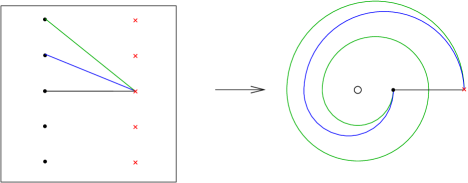
Returning to the general case of an atomic Lefschetz fibration , choose a base point so that . By choosing different logarithms of , we may index the set of isotopy classes
of -admissible paths from to where
| (11) |
It is sometimes useful to vary the basepoint , so we will frequently use the notation in equation (11). However, when we fix a base point , we will take be the unique logarithm of for which . We write for . Three of the logarithmic paths and their images are illustrated in Figure 4.
Definition 6.
Given an atomic Lefschetz fibration , the -unfolded Fukaya-Seidel category of is the category where is the pullback of along and for .
As the next proposition indicates, the -unfolded category of is independent of the choice of cut and can be computed directly from the vanishing cycles associated to . To make this computation, we first choose a natural distinguished basis of paths and fix a coherent brane structure on their associated vanishing cycles. First we equip the vanishing thimble with an arbitrary Lagrangian brane structure. This induces a brane structure on and we write the associated object as . For , we then equip with a brane structure induced by the one on . This can be done by performing symplectic monodromy around exactly times, which is a graded symplectomorphism. Write
| (12) |
for the associated collection of objects in .
Proposition 2.
For any , there is an equivalence of categories
Proof.
Consider the pullback of along .
| (13) |
The critical values of are the -th roots of . For any choice of , let be the -th root which follows clockwise and take for . Using unique path lifting of with respect to the basepoint lifting to , one obtains a unique lift for every . It is clear that if , so that is a distinguished basis of paths for . Take to be the respective collection of vanishing cycles in . Note that yields a symplectomorphism from to and the symplectic connection of pulls back to that of . Thus the vanishing cycle is mapped isomorphically to via so that induces an equivalence of categories from to taking to for . The result for then follows from Definition 4. For general , we note that monodromy about induces an symplectomorphism from to itself which carries to so that, for varying , the associated directed subcategories with respect to are equivalent. ∎
The class of atomic LG models that we consider arises from pencils on Kähler varieties. We utilize this additional structure and make a definition.
Definition 7.
Let be a projective variety with ample line bundle . Given two linearly equivalent, effective divisors , such that is a normal crossing divisor, we say the pencil
is an atomic Lefschetz pencil if its restriction to is an atomic Lefschetz fibration.
When an atomic Lefschetz fibration arises as an atomic Lefschetz pencil, one may define and utilize additional invariants. Assume that, for or , where is an irreducible component of . Let and, for any , extend the pullback in equation (13)
| (14) |
by adding . Observe that for , is regular on the pullback of in the partial compactification of . Now, let
be the disc with boundary and removed as in the right hand side of Figure 5. We equip with a strip like end near which is a trivialization for which and for (see [26, Section 8d]). Let and be the union of the counter-clockwise parallel transports of along the boundary of . So gives a Lagrangian boundary condition for the fibration and one can consider the zero dimensional component in the moduli space of sections of
| (15) |
For any such section , we have that, where is Hamiltonian isotopic to . Moreover, for every we define a subspace of which isolates those sections for which . Precisely, for , we take
Then we obtain the partition
| (16) |
Using the Pin structure on to orient , the usual TQFT formalism applies in this setting to show that the signed count for coboundaries so that, for all , one obtains the invariant
where
| (17) |
This additional invariant for atomic Lefschetz pencils will be used in the induction proof for Theorem 3 in Section 3.5.
3.2. Circuit LG models
In this section we will review the mirror potential of an elementary birational cobordism and state the main theorem of this paper. Consider satisfying equations (2) and of signature . If necessary, permute the coordinates of so that for and for . The volume of is defined to be the constant
| (18) |
Let be homogeneous coordinates of . For any subset take
| (19) |
to be the associated coordinate plane. Recall that the -dimensional pair of pants is the subvariety
| (20) |
We will write for the closure of in . Let and define the divisors and sections
| (21) |
Observe that is the base locus of the associated pencil .
Definition 8.
The circuit pencil associated to on is defined by the map given by . The circuit LG model is the restriction of to the pair of pants .
Lemma 1.
The circuit LG model is an atomic Lefschetz pencil with unique critical point and critical value .
Proof.
This follows at once from a basic computation of the critical points for . Indeed, wedging the exterior derivative of the constraint and gives
So a critical point of satisfies for all and . This implies the result that is the unique critical point. To see that it is a Morse critical point, one applies the complex Morse Lemma by computing the Hessian of and observing that it is non-degenerate. We cite [12, Proposition 2.13] for this computation. ∎
To define the Fukaya-Seidel category associated to , and in particular to consistently grade the morphisms between Lagrangians, we specify a non-zero holomorphic volume form. We will keep some flexibility here, but index the possible choices by using our function from equation 3. Fix the meromorphic -form
which is holomorphic and non-zero on . To obtain a non-zero -form on , assume that and take
to define
| (22) |
For later use, we express in local coordinates where and pull back via the chart . Here a short computation shows
| (23) |
The -model category associated to may then be defined as follows.
Definition 9.
Suppose are balanced, , and . Denote by the directed subcategory where with grading induced by . If , let and write for the -unfolded Fukaya-Seidel category .
The definition of has an ambiguity up to Hamiltonian deformations of , although it is well defined up to quasi-equivalence. To remove this ambiguity, given a collection for which is Hamiltonian equivalent to in , we will say is a Hamiltonian representative basis of and assert that is defined by . The main theorem of the paper gives an explicit description of in cases where is bounded by the volume of .
Theorem 3.
Given balanced and with , there exists a Hamiltonian representative basis of defining and an isomorphism
| (24) |
for which
-
(i)
,
-
(ii)
takes the monomial basis vectors to the canonical basis of intersections.
Furthermore, for any , one has
| (25) |
This theorem will be proved by induction on in the following sections. For now, we note that Theorems 3 and 2, yield the following important corollary.
Corollary 2.
The categories and are equivalent.
This corollary gives further evidence of the link between birational geometry on the -model side and degenerations on the -model side of mirror symmetry. As a special case of this corollary, we obtain the folklore result.
Corollary 3.
The homological mirror symmetry conjecture holds for weighted projective spaces .
This result was proven in [5] for weighted projective planes and [15] for ordinary (unweighted) projective space.
Proof of Corollary 3.
Given positive weights with take , and . The VGIT for this collection of weights is a transition from to the vacuum . By equation (6), we have that .
On the -model side, recall from equation (9) that . Write for the divisor in . Consider the map obtained by taking
It is not hard to see that is simply the quotient by . Using the definitions of the mirror potential of in Example 4 and of the quotient from equation (10), one observes that . This yields the fiber square
In particular, both the Fukaya-Seidel category and are quasi-equivalent to the category of twisted complexes of the algebra generated by vanishing cycles of a distinguished basis of paths for . This yields the equivalence , and, applying Corollary 2, finishes the proof. ∎
3.3. One-dimensional case
In this section we will consider the case of . Up to isotopy, we will describe the thimbles of for any given and utilize Proposition 2 to prove equation (24) in Theorem 3. We will first establish a bit of notation.
Let be a small real number and be a smooth function satisfying
-
(1)
is monotonically decreasing,
-
(2)
for and,
-
(3)
for .
Now suppose is the surface with a point and a local unit disc chart around with coordinate . Given a real number we define a twist of by taking
| (26) |
and extend to by taking the identity outside of . If are a tuple of distinct points and are real numbers we write for the composition, which is well defined assuming that the local coordinates were chosen to be disjoint.
We now state a basic result for . We write for the -th roots of unity in .
Proposition 3.
Assume that has signature . Then there is a trivialization and for which
-
(i)
the fiber ,
-
(ii)
the vanishing thimble of equals the line segment
-
(iii)
the vanishing thimble of is isotopic to the curve
Proof.
Consider the coordinate with the chart . Then the circuit potential has the form
| (27) |
One checks that the critical point of is with value as in Lemma 1. Locally around , . Take to be sufficiently negative and choose the basepoint . We can identify the fiber with the -th roots of the positive real number . For small , we may perturb the coordinate near so that identifies with . Using the coordinate , we obtain
so that an identical argument yields an identification of the fiber with the -th roots of the positive real number where again . Thus Proposition 3(i) holds.
Now, depending on the parity of and , the graph of the restriction of to the real locus is one of the four possibilities in Figure 6. In each case, we have that the interval maps to the connected component of which contains the critical point . But by Definition 8, the vanishing thimble of a path for a Lefschetz fibration with domain a Riemann surface equals the component over the path containing the critical point. This verifies the claim 3(ii).
For 3(iii), we note that has zeros of order and at and respectively. Thus, in local coordinates around and , the fiber equals . As is isotopic, relative its boundary, to the concatenation of with a -fold counter-clockwise loop around , we have that the vanishing thimble is that of twisted by (here we assume that is sufficiently small so that the fiber is close to and in local charts). ∎
Proposition 4.
Theorem 3 holds in dimension .
Proof.
We first describe the equivalence in equation (24). By Proposition 1, it suffices to show this for with signature as the case of is Koszul dual. On generating objects, we define where is the vanishing cycle endowed with a brane structure relative to . For , the vanishing cycles and the fiber are both zero dimensional. Furthermore, by Proposition 3(i) and 3(iii) we have that there is a small and a trivialization for which where
The grading of the vanishing cycles and their intersection points is obtained by considering the grading of the vanishing thimble relative to at and . Given the trivialization on , we have that
Proposition 3(ii), we may grade by taking a real valued argument for . Precisely, letting be the phase of at on , this gives
Proposition 3(iii) gives the remaining thimbles in terms of the monodromy twists of . To accomplish transversality between two vanishing thimbles, taking small , we slightly perturb to near by rotating . As, the order of at and is and respectively, one observes that the induced grading of is then
Given if intersects amongst the points , respectively , we denote the intersection , respectively . Then
The absolute index of these intersections point gives their grading and, for and using [26, Section 13c], they are computed as
Taking the case of , degree considerations imply that the differentials and higher compositions all vanish. Changing , however, does not affect the moduli spaces determining these compositions, so they will vanish for any choice. On the other hand, an elementary perturbation argument shows that
where denotes the composition determined by the -structure. In this case, agrees with the second map, but generally may differ by a sign depending on the parity of the first factor (see [26, Section 1a]).
One then extends the functor to morphisms by taking
It is clear that then defines the isomorphism of categories specified in (24) and satisfying Theorem 3(i) and 3(ii). We note that, since and is a morphism from to we do not encounter this morphism in the -unfolded category .
We now show that equation (25) holds for . This can easily be seen when has signature or , and we give the argument for the former case. Using the trivialization of , denote and for the compactification points on . The divisors and from Definition 7 are then and respectively. Consider the pullback in equation (14) with . Write for a small disc around and for . For a local disc chart around we have the diagram
| (28) |
where the is the union of discs with common intersection point . Parameterizing the -th disc by we have that where and .
Now, corresponds to a point of the form so that the pullback of along is on the boundary of the radius circle on the -th disc in . Thus the moduli space contains the unique section sending to the in the -th component. It is clear that is the unique section of with boundary condition containing the boundary of the -th disc. To see that is unique up to isomorphism in , assume otherwise and compose with and to obtain a map . Since sends the boundary of to , the maximum principle implies that . This in turn shows that and . It follows that
An identical argument applies for and which verifies equation (25) and the proposition. ∎
To conclude this section, we describe holomorphic polygons in with boundary conditions labeled by thimbles and their intersection points. We first establish the general notation. Let be a symplectic surface with a regular compatible complex structure and a finite set of points. Suppose is an ordered set of graded Lagrangian submanifolds, possibly with boundary, such that and . We equip each with a Hamiltonian for which and write for their union. Take to be the time flow map of
Definition 10.
Given a finite ordered collection of Lagrangian branes along with Hamiltonians , we call the pair generic if
-
(i)
Lagrangians in pairwise intersect transversely,
-
(ii)
pairwise intersections have a constant number of points for ,
-
(iii)
for every subset and every , we have that are transverse submanifolds in .
By property 10(ii) we can label the intersection points of two Lagrangians for any time by . We write the graded vector space generated by this intersection as
Now suppose that is a pointed disc with marked points oriented counter-clockwise. Given a set map , we say that is a labeled pointed disc. Denote the arc on from to as .
Definition 11.
Given a labeled pointed disc and a generic pair we say that a -holomorphic map is directed relative to if
-
(1)
the Maslov index of is ,
-
(2)
,
-
(3)
is an increasing function.
If we write
Turning our attention back to the one-dimensional circuit, we consider and write
Using Proposition 3, we now describe a collection of paths
| (29) |
in isotopic, relative to , to the thimbles in . Utilizing the parametrization , take . For any define the line segment
via
| (30) |
Define the path via .
Proposition 5.
The path is isotopic to in relative to . Furthermore, for , we have
| (31) |
Proof.
Consider the space and the cover where we have identified with . By Proposition 3(i) we have that is . Furthermore, one observes that the twist map on lifts to a map isotopic to the shear map
| (32) |
Thus by Proposition 3(iii) we have that is isotopic to proving the first claim.
To verify equation (31), one checks that there is a one to one correspondence between points in and integers for which . As the real values of and are and respectively, an intersection point of the latter has the form implying . As this implies
| (33) |
The number of such integers satisfying this inequality is precisely . ∎
We now label the intersection points between and . For , we write
| (34) |
and write . Then applying the arguments from Proposition 5, we see that
| (35) |
With this labeling, we are able to detail the directed discs relative to the collection .
Proposition 6.
There are Hamiltonian perturbations for for which
-
(i)
is generic,
-
(ii)
any directed relative to must be a holomorphic triangle, a constant bigon, or a constant polygon with image in .
-
(iii)
for and any and there exists a unique directed triangle with
(36) and every non-constant holomorphic triangle satisfies such an equation.
Furthermore, for a non-constant with boundary condition (iii) either
-
(a)
has the same sign as and the image of is contained in or,
-
(b)
has the opposite sign as and the image of contains .
Proof.
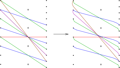
Define to be a sufficiently small Hamiltonian which rotates clockwise around for small time and yields a small twist map for . We may choose so that the tangent line of at any point has slope approximately equal to , which is equal to the slope of . Such a collection of perturbed Hamiltonians is illustrated in Figure 8. It is clear that, for generic choices of twists, the collection makes generic.
Now, for any directed , we have that there is a lift which is unique up to a translation by . In order for to be a Maslov index disc, either is constant or it is a convex polygon with boundary edges lying on for . In the former case, by Definition 10(iii) the curves intersect transversely in the interior of . In particular, no three of them intersect in a single point in , so that any directed constant map with more than two boundary components must have image in .
For the latter case, suppose is the labeled pointed disc domain of with marked points . Working on the cover of , take to be the quadratic holomorphic form given by (different choices will not affect this argument). Each Lagrangian can be graded by choosing a continuous family real arguments for which, by our choice of perturbations, we may take to be arbitrarily close to . The absolute index (see [26, Section 13c]) of the intersection point for is then
For we have . Thus, for an arbitrary holomorphic disc with boundary conditions in , we have for all . However, since is directed, is an increasing function which implies that for all . Writing for the Maslov index of , this then implies that
so that the only non-constant directed maps must have and are holomorphic triangles.
To show 6(iii), it suffices to consider the lift of a holomorphic triangle with domain the pointed disc where , and . Using the Hamiltonians in , we may assume the map has been perturbed so that the boundary is mapped to versus . This may collapse certain triangles to constant maps, but otherwise it deforms a holomorphic triangle to a convex triangle. Assume for and choose a lift so that the arc from to is mapped to . Then the image of is bounded by , and where
Then is equivalent modulo to so that which verifies the claim. Conversely, one easily shows that and satisfying the respective bounds in inequality (33), satisfies this inequality as well and there is a holomorphic triangle for which equation (36) holds.
For claims 6(a) and 6(b) we simply observe that if and have the same sign, then so does and the holomorphic triangle lies in the positive or negative real half plane and does not contain . On the other hand, if and have opposite signs, then the triangle intersects in an interval. But since, for every , intersects in we have that this interval must intersect non-trivially so that the image of contains . ∎
Proposition 6 is closely related to the calculation of the wrapped Fukaya category for the cylinder and the pair of pants [3, 14]. However, there are two minor differences which prevent one from referencing such computations directly. First, the paths are compact paths in a non-compact surface, versus the case of a Lagrangian with Legendrian boundary (or a non-compact Lagrangian with a cylindrical end [2]). Secondly, the lengths of these compact paths are asymmetric about circle of radius , making the book-keeping of intersections slightly more delicate.
3.4. Circuit Lefschetz bifibrations
In this section we will prepare the groundwork to perform the induction step for the proof of Theorem 3. An essential ingredient in this step is the use of matching paths and Lefschetz bifibrations which factor the circuit LG model . We first define a slight variant of Lefschetz bifibrations adapted to the setting of pencils on Kähler manifolds.
Let be a complete Kähler manifold with four effective, smooth normal crossing divisors such that and are linearly equivalent to and respectively. We call the pencils associated to and the vertical and horizontal linear systems respectively. Write and for the base loci of these linear systems and , for the induced maps. For we say the divisor is an irregular horizontal divisor if it does not transversely intersect . Finally, we write for the product .
Definition 12.
The collection is said to generate a Lefschetz bipencil if
-
(i)
and are components of ,
-
(ii)
is a Lefschetz pencil,
-
(iii)
there are finitely many irregular horizontal divisors ,
-
(iv)
the closure of the critical locus does not intersect and satisfies
for all .
If generates a Lefschetz bipencil, then it can be used to obtain an exact symplectic Lefschetz fibration as defined in [26, Section 15c]. Consider the spaces
The exact symplectic structure on can be defined by taking the Kähler potential . Writing for the projection to the first coordinate, we then obtain the sequence of maps
| (37) |
Because , the Fukaya-Seidel category of differs from the Lefschetz pencil and we will need to reincorporate the excised divisors into the picture in order to relate these categories. We will do this in the next section, but first we describe our main example of a Lefschetz bipencil.
Let and satisfy equations (2). Assume has signature with and take . We consider the collection of effective divisors where the vertical divisors are given from equation (21) and
With this data, we have that and .
Proposition 7.
The collection on generates a Lefschetz bipencil with irregular horizontal divisors . Furthermore, the critical points and values of are
| (38) | ||||
| (39) |
Proof.
One verifies Definition 12(i) immediately from the definition of the divisors in while 12(ii) was observed in Lemma 1. For property 12(iii) we take coordinates and observe that for , we have that . A check shows that the intersection with the support of then gives transverse coordinate hyperplanes. On the other hand at , while at , has a non-transverse intersection with at the point .
For the last property 12(iv), we first compute the critical points of in . Letting , we have
| (40) |
Let and observe
which is non-zero for all . Next, one checks that if and only if
By Proposition 7 we have that generates a Lefschetz bipencil and that the induced diagram
is a symplectic Lefschetz bifibration where and we define as the restriction of to . In this diagram, we have implicitly identified with . As we will utilize this identification shortly, we make it explicit by taking
Fixing more notation, we write for and, noting that , for any we write for the partial compactification . We then extend to a map by sending to zero. These partial compactifications then fit into the following commutative diagram.
| (41) |
We will denote the fibers of , and over as , and respectively.
Our next task in the induction argument is to understand the Lefschetz bifibration purely in terms of lower dimensional circuit potentials. Given balanced , define lower rank lattice elements
| (42) | ||||
The elements and clearly satisfy the equations (2) and are of signature and respectively. If is balanced then one easily checks that and are balanced. Also take to be the function
Writing for the restriction of to , we state the following proposition.
Proposition 8.
There is an isomorphism
for which . Furthermore, for any fibers and fit into the pullback diagrams
| (43) |
Proof.
Define the maps and via
where . One easily computes that and yield a pair of inverse isomorphisms between and . To see that one utilizes the coordinate representation of given in equation (23).
To see that induces the fiber squares in (43), we have that if and only if
Thus, and restrict to inverse isomorphisms between and yielding the left hand diagram. The extension to is immediate from the fact that maps to via . ∎
A basic corollary of Proposition 8 gives a description of the critical values of in terms of the one-dimensional circuit potential studied in Section 3.3.
Corollary 4.
For any , the set of critical values equals the fiber .
Proof.
Using Proposition 8 and Corollary 4, we will accomplish the basic task of identifying the vanishing cycles of associated to the paths defined in equation (11). To do this, we will recall and apply the general machinery of matching paths and matching cycles (see [26, Section 16]). As our Lefschetz bifibrations satisfy particularly strong properties, we will only need a basic version of this machinery which we now discuss. First, let be the closed upper half-disc , its upper boundary and its interior.
Definition 13.
Let be a Lefschetz fibration from a Kähler surface which restricts to a Lefschetz fibration on a complex curve . Given a -admissible curve from to , an embedded path will be called a matching path of if there exists an embedding such that
-
(1)
,
-
(2)
is an embedding into ,
-
(3)
for all ,
-
(4)
.
Matching paths can be visualized by imagining the movie of points in the fiber with starting at and ending at . As is a Lefschetz fibration, at one of the points in has multiplicity and for small , it separates into two points in . Drawing a path between these points and continuing it via a smooth isotopy until yields a matching path to . Here it is important that the interior of the path never intersects a point of . We note that matching paths are defined up to relative isotopy in .
In fact, the notion of a matching path for an ordinary Lefschetz fibration is a priori distinct from the above definition. In this more basic scenario, suppose is a path with , and let be the restrictions . Then we say that is a matching path if the vanishing cycles and are Hamiltonian isotopic Lagrangian submanifolds of the fiber . The main advantage of having a matching path is that, assuming one performs a fiberwise Hamiltonian isotopy of vanishing cycles along , one may glue the vanishing thimbles together to obtain a Lagrangian sphere . The sphere is called the matching cycle of . We now recall the following result relating matching paths, matching cycles and matching paths of admissible paths.
Proposition 9.
[26, Lemma 16.15] Let , and form a Lefschetz bifibration and . Assume is a -admissible path from to . Then:
-
(1)
is a -admissible path,
-
(2)
if is a matching path of , then it is a matching path for ,
-
(3)
for an appropriate isotopy , the matching cycle is isotopic, as a framed Lagrangian sphere in , to the vanishing cycle .
In order to utilize Proposition 8 to produce matching paths, it will be helpful to notationally distinguish , and -distinguished paths. Given any with and , take and let be the -admissible path defined in equation (11). Let satisfy and choose with . Taking , we define -dependent admissible paths and via
| (44) |
The -subscript is redundant, and will occasionally be omitted, but will be nonetheless useful to distinguish different admissible paths. Noting that , one also may easily compute the relation
| (45) |
Proposition 10.
Let , , and with and . Then:
-
(i)
for and , the -admissible curve is -admissible,
-
(ii)
the vanishing thimble is a matching path of .
Proof.
To prove 10(i), we observe that equation (39) of Proposition 7 shows that is in fact equivalent to yet another one-dimensional circuit potential. Thus by Lemma 1, there is a unique Morse critical value which must equal the critical value of implying that any -admissible path is also -admissible. In the terminology of [26, Section 15], we see that the fake critical value set is empty so that for every , the map is a Lefschetz fibration.
For 10(ii) we show there exists a map satisfying Definition 13 with . To avoid notational confusion, take to be the vanishing thimble of with respect to the function . As is Morse, there is a parametrization for which . We will extend to .
First we take and let . For , define to be a smoothly varying parameterization of the vanishing thimble of . By the definition of , we have
Thus by Corollary 4 and the fact that we have that .
As tends to , tends to which implies that is approaching a constant path. In turn, the vanishing thimble, parametrized by is also approaching the critical point . This implies that sends its endpoints to the vanishing thimble of over and in particular to the second coordinate of . Thus we may extend as
The fact that satisfies Definition 13 to give the matching path of is an immediate consequence of its construction. As parametrizes the thimble , the conclusion of the proposition follows. ∎
Propositions 9 and 10 then yield descriptions of the vanishing cycles of the -admissible paths as pullbacks of the vanishing thimbles of along the one-dimensional circuit potential . The language and notation for the procedure of doubling thimbles to obtain spheres was introduced in Definition 3. This description gives the final preparatory input to accomplish the induction step in the proof of Theorem 3.
Proposition 11.
Suppose with and , and let . Then,
-
(i)
the path is -admissible,
-
(ii)
Taking to be the vanishing thimble of over , the vanishing cycle is Hamiltonian isotopic to .
Proof.
The first claim follows from the fact that is the unique critical value of which, by equation (44), also equals . For 11(ii), one applies Propositions 9 and 10(ii) to see that the vanishing cycle is isotopic to a matching cycle of over the matching path . But, by equation (45), and, more precisely, is the unique pullback of along which contains the unique critical point of . Using Proposition 8, is the matching cycle fibered over implying it is Hamiltonian isotopic to . ∎
With these propositions in hand, we perform the induction step and complete the proof of our main theorem.
3.5. Proof of Theorem 3
Assume the claim is true for any satisfying equations (2) with . Given , use equations (42) to define and . We will assume that the signature of is with , otherwise take and apply Koszul duality.
Choose so that , and set a basepoint of as . We fix the basepoint of where was defined before equation (44).
Note that so that for we may apply the induction hypothesis for . Thus there is a collection of Lagrangian vanishing cycles corresponding to a distinguished basis of paths and an isomorphism
| (46) |
for which .
We will now specify a basis for along with an isomorphism to . From Proposition 11 the vanishing cycles are isotopic to matching cycles of over the thimbles . Using the parametrization from Proposition 3, these thimbles were shown to be isotopic to in Proposition 5, or their Hamiltonian perturbations in Proposition 6. We recall that was a path where is defined by the condition
| (47) |
for and was defined in equation (30).
The intersections of these thimbles were found in equation (35) to be
where . Thus, perturbing the matching cycles so that they lie over , we may partition the intersection to obtain a decomposition of the morphism group
| (48) |
Here is generated by the intersections of lying over relative to . For the moment we fix and let
| (49) |
so that is uniquely written as . Also define the constants
| (50) |
These constants will be used repeatedly to denote shifts in weight and degree, respectively.
Claim 1.
For any , there is an isomorphism
| (51) |
Proof of Claim 1.
First, note that either or . If , then the intersection point of the paths and in lies in the unit disc (see equation (30)). There are two sub-cases to consider here. First, if and then occurs at the endpoint of the matching paths implying the vanishing spheres intersect in a point. In this case, so that is isomorphic to up to the grading. The grading shift will follow from the discussion of the second sub-case where .
For , the line segments of the lifts and for lie in the real negative half plane and intersect at . By equation (47), the constant satisfies for any . Define two paths, from to , and from to . Write for the concatenation of with (where the negative sign indicates a reversed orientation). Note that lies in the negative real half plane. These paths are illustrated on the left in Figure 9.
Recall from equation (27) that has an order ramification at so that the image of has winding number as in the upper right side of Figure 9. Applying to and give -admissible paths , from to . Calculating winding numbers, one observes that with , the paths and are isotopic to and respectively, for an appropriate in the -plane.
As the winding number of concatenated with is and since it lies in the disc of radius , it is isotopic to a concatenation of and where the isotopy is obtained via a theta varying twist map (defined in equation (26)). Take to be the base point for the paths and . Performing symplectic parallel transport along the fibers over the isotopy gives a symplectomorphism from to which, upon pulling back relative to in the fiber product (43), sends the vanishing cycles and to and , respectively. By incorporating the Hamiltonian isotopy into a fiberwise perturbation over and near , we may assume this identifies these pullbacks with the fiber of the matching cycles and over . This identifies the Floer complex with .
Finally, to observe the shift of in the grading, we grade so that the isomorphism
respects the grading. We note that this is possible by the description of given in Proposition 8. Utilizing this description again, one observes that performing symplectic parallel transport relative to along a counter-clockwise path once around the origin yields a grading shift of (as has order at the origin). The winding number of the path from to along and then to along is precisely . Thus the grading shift for is .
The case of yields an identical argument, with the exception of working with and the positive half plane, so we omit this repetition. ∎
We note that is independent of in the sense that the monodromy of obtained by winding around the origin times takes to inducing an equivalence on . From the construction, it is clear that . Taking , and using equation (48) , we obtain the isomorphism
| (52) |
Turning to the -model, notationally distinguish and by taking the basis for and for , and defining and . Here, weights and degrees are assigned according to equation (4) with respect to , and , respectively. Given , define
For and satisfying take , as in equation (49), so that , and as in equation (50). Consider the space of homogeneous elements of weight and define a projection
by taking
The intuition behind is to identify with and divide by or , thereby decreasing the weight (and degree) of by or (and ) respectively. It is an elementary check to show that the direct sum of these maps yields an isomorphism
| (53) |
By Definition 2 of , for any with and , there are natural maps which define the isomorphism in the following commutative diagram
where the direct sum is for integers satisfying .
Given this preparation, we are now able to extend the functor to morphisms. For any define
as the composition
By Claim 1, equation (53) and the induction hypothesis, we see that is an isomorphism of graded vector spaces. To conclude that is an isomorphism, we need only show that it commutes with multiplication.
Claim 2.
defines a functor. In particular, for and we have
| (54) |
Proof of Claim 2.
We start on the -model side with an observation. Suppose and for . If denotes the -th -multiplication map in then for we have
This follows from the observation that we may choose a regular complex structure for which is holomorphic (one may prove regularity by induction). Applying Proposition 6(i) to obtain a generic collection of Hamiltonian perturbations for we may identify the vanishing cycles as matching paths over the transversely intersecting so that any holomorphic disc with Lagrangian boundary conditions on must map via to a directed disc in relative to the perturbed collection . By Proposition 6, such discs are either constant or holomorphic triangles. In the former case, (where we again drop the perturbation term from the notation), but as no other vanishing cycle lies over this point, we have that must be a bi-gon in . By the induction hypothesis utilized in the previous claim to identify the fibers of the matching cycles over with and , the differential on the Floer complex is zero.
Before proceeding further, let us simplify and detail our notation by taking , , , and . We will assume that and where and are monomials in . Applying Proposition 6(iii) we observe that
Moreover, we have two potential scenarios as outlined in Proposition 6(a) and 6(b).
Case 1: and have the same sign.
We assume as the proof when is analogous. Then we may uniquely decompose and so that for . Let and be the associated monomials in . Then, by the definition of one easily shows
| (55) |
Now, letting , Proposition 6 implies there is a unique directed disc in which bounds and and takes the marked points to for . This is illustrated in the logarithmic pullback on the left hand side of Figure 10. Write for its image in the -plane, take to be its vertices and its pointed disk which we equip with strip like ends. The moduli space of discs with boundary conditions whose strip like ends converge to , and then equals the moduli space of sections of over the disc with boundary conditions on the image of the vanishing cycles in . Since is a contractible disc, may be globally trivialized, using symplectic parallel transport along the boundary. The moduli space of sections with boundary conditions given by this transport map is isotopic to one with constant Lagrangian boundary conditions given by taking along , along and along . It follows from the construction of that the component of this moduli space defining has strip like ends converging to and where and . Such a space of sections is cobordant to the moduli space defining in which, by the induction hypothesis, is cobordant to a single point defining where . This implies
| (56) |
Thus, collecting equations (55) and (56) yields
which validates equation (54) and the claim for the first case.
Case 2: Either or .
The case of and having opposite signs reduces to this case using associativity and a basic induction argument. The two sub-cases are proved in analogous ways, so we assume as illustrated in the bottom right triangle in Figure 10. Using the isomorphism defined in equation (52) we have that the morphisms and where both represent the identity morphism. As is a unital functor, this implies that and where are identities. By the definition of we have that and . This implies that and . Thus, to prove the claim, we need only show that
| (57) |
By Proposition 6(b), the product is a linear combination of the set of intersection points of and lying over or . In other words, there are moduli spaces for which
| (58) |
Let us consider the spaces in more detail. Take to be the holomorphic triangle in with boundary along and . One can easily compute that there exists exactly one element and that is a holomorphically embedded triangle in (after applying the appropriate generic Hamiltonian perturbations ). Note that we are now working in the fiber as opposed to and applying the right hand diagram in Proposition 8. The moduli space of consists of the space of sections of over with boundary conditions and over and respectively. As the paths in are matching paths over which the Lagrangians are matching cycles, and as the intersections and occur over the endpoints, the Lagrangian boundary conditions near and are exponentially converging and, applying an implicit function theorem (see, for example, [23]), we may round the corners of to obtain a domain as illustrated in its logarithmic preimage in Figure 11.
The Lagrangian boundary condition thus obtained is the pullback of near the lower boundary of the strip like end at , along with its parallel transport counter-clockwise around . Sections of over with this boundary condition gives moduli space cobordant to and, as is regular on away from , we may isotope to be a small disc around , simultaneously performing parallel transport to maintain the Lagrangian boundary condition of in the lower boundary near . Take to be the inverse image of . As has a order ramification at , using Proposition 8, we have that the pullback
is symplectically isomorphic to the pullback in equation (14) with and . By performing symplectic monodromy, we may replace the Lagrangian boundary condition of the symplectic transport of with . Then from equation (16), moduli space of sections decomposes as
where . Since , the definition of in equation (17) gives
To conclude the proof of Theorem 3, we only need to verify equation (25) for and . Indeed, by permuting the indices, this argument then gives the result for any with and by inverting (which transposes the signature of ), the argument can be run for .
We recall the necessary preliminaries to define in this case. The bottom row of diagram (41) gives that map factors through . Take to be the pullback from equation (14) illustrated on the left of diagram (59).
| (59) |
Let be a small pointed disc of radius less than with marked point equipped with the moving Lagrangian boundary condition of near and moving counter-clockwise by parallel transport. Write for this boundary condition and for , . Let be the function with the assumption that as approaches from a clockwise direction. By Propositions 8 and 10, the image of via is which is a matching cycle relative to over the matching path and vanishing thimble .
From equation (16), and the fact that only the divisor was added to (as opposed to ) the moduli space of sections of over equals
Now, equation (25) follows from two observations.
First, we note that for there exists a section . To see this, recall from the proof of the previous claim that corresponds to the intersection lying over the endpoint intersection via . In particular, lies in the critical point set and, as moves counter clockwise around , since is a matching cycle over which must contain the critical endpoint over , there is a map . By equation (59), has winding number , and using the explicit form of in equation (38), we see that it intersects with order . Thus the closure of over is a smooth complex curve and can be completed to a holomorphic section. We observe that, since restricting to is a one-dimensional circuit potential, this argument is identical to that given in the proof of Proposition 4.
For the second observation, we check that is unique. Given any , consider defined to by . Then for any , we have where was defined as the shear map in equation (32). For , the Maslov index of must be which implies it has a first order zero at . In particular, is well defined with image in and vanishing winding number about implying that one may take a logarithmic branch . Extending to a line for every , the boundary conditions of are such that . This implies that the Maslov index of and thus is constant at the intersection . Thus and . Consequently, for every , lies over the same endpoint of the matching path as . But as was observed above, there is a unique point in mapping to such a critical value of implying that . By unique analytic continuation, and
| (60) |
By the definition in (17), we have is for and otherwise. This validates equation (25) and concludes the proof of Theorem 3.
References
- [1] M. Abouzaid. Morse homology, tropical geometry, and homological mirror symmetry for toric varieties. Selecta Math., 15:189–270, 2009.
- [2] M. Abouzaid. On the wrapped Fukaya category and based loops. J. Symplectic Geom., 10:27–79, 2012.
- [3] M. Abouzaid, D. Auroux, A. Efimov, L. Katzarkov, and D. Orlov. Homological mirror symmetry for punctured spheres. J. Amer. Math. Soc., 26:1051–1083, 2013.
- [4] D. Auroux, L. Katzarkov, and D. Orlov. Mirror symmetry for del pezzo surfaces: vanishing cycles and coherent sheaves. Invent. Math., 166:537–582, 2006.
- [5] D. Auroux, L. Katzarkov, and D. Orlov. Mirror symmetry for weighted projective planes and their noncommutative deformations. Ann. of Math., 167:867–943, 2008.
- [6] M. Ballard, C. Diemer, D. Favero, L. Katzarkov, and G. Kerr. The Mori program and non-Fano toric homological mirror symmetry. Trans. Amer. Math. Soc., 367:8933–8974, 2015.
- [7] M. Ballard, D. Favero, and L. Katzarkov. Variation of geometric invariant theory quotients and derived categories.
- [8] A. Beilinson. Coherent sheaves on and problems in linear algebra. Funktsional. Anal. i Prilozhen., 12:68–69, 1978.
- [9] A. Beilinson, V. Ginzburg, and W. Soergel. Koszul duality patterns in representation theory. J. Amer. Math. Soc., 9:473–527, 1996.
- [10] A. Bondal. Helices, representations of quivers, and koszul algebras. In Helices and vector bundles: Seminaire Rudakov, volume 148 of Lecture Note Ser., pages 75–95. London Math. Soc., 1990.
- [11] A. Bondal and D. Orlov. Semiorthogonal decomposition for algebraic varieties. 1995.
- [12] C. Diemer, G. Kerr, and L. Katzarkov. Symplectomorphism group relations and degenerations of Landau-Ginzburg models. 2015. JEMS to appear, arXiv: 1204.2233.
- [13] B. Fang, C. Liu, D. Treumann, and E. Zaslow. T-duality and homological mirror symmetry for toric varieties. Adv. Math., 229:1875–1911, 2012.
- [14] K. Fukaya, P. Seidel, and I. Smith. Exact Lagrangian submanifolds in simply-connected cotangent bundles. Invent. Math., 172:1–27, 2008.
- [15] M. Futaki and K. Ueda. Tropical coamoeba and torus-equivariant homological mirror symmetry for the projective space. Comm. Math. Phys., 332:53–87, 2014.
- [16] I. M. Gelfand, M. Kapranov, and A. Zelevinsky. Discriminants, resultants and multidimensional determinants. Birkhäuser Boston, Inc., 2008.
- [17] A. Givental. Homological geometry and mirror symmetry. In Proceedings of the International Congress of Mathematicians, volume 1, pages 472–480. Birkhäuser, Basel, 1995.
- [18] D. Halpern-Leistner. The derived category of a GIT quotient. 2013.
- [19] K. Hori and C. Vafa. Mirror symmetry. 2000.
- [20] Y. Kawamata. Derived categories of toric varieties. Michigan Math. J., 54:517–535, 2006.
- [21] G. Kerr. Weighted blowups and mirror symmetry for toric surfaces. Adv. Math., 219:199–250, 2008.
- [22] K. Lefèvre-Hasevawa. Sur les -catégories. PhD thesis, Université Paris 7, 2003. arxiv:math.CT/0310337.
- [23] D. McDuff and D. Salamon. -holomorphic curves and symplectic topology, volume 52 of Colloquium Publications. AMS, 2004.
- [24] R. Morelli. The birational geometry of toric varieties. J. Alg. Geom., 5:751–782, 1996.
- [25] M. Reid. What is a flip? 1992.
- [26] P. Seidel. Fukaya categories and Picard-Lefschetz theory. Zurich Lectures in Advanced Mathematics. European Mathematical Society (EMS), Zürich, 2008.
- [27] K. Ueda. Homological mirror symmetry for toric del Pezzo surfaces. Comm. Math. Phys., 264:71–85, 2006.
- [28] J. Włodarczyk. Birational cobordisms and factorization of birational maps. J. Algebraic Geom., 9:425–449, 2000.