Direct frequency comb laser cooling and trapping

Abstract

Continuous wave (CW) lasers are the enabling technology for producing ultracold atoms and molecules through laser cooling and trapping. The resulting pristine samples of slow moving particles are the de facto starting point for both fundamental and applied science when a highly-controlled quantum system is required. Laser cooled atoms have recently led to major advances in quantum information García-Ripoll et al. (2005); Bloch et al. (2012), the search to understand dark energy Hamilton et al. (2015), quantum chemistry Zhu et al. (2014); de Miranda et al. (2011), and quantum sensors Dickerson et al. (2013). However, CW laser technology currently limits laser cooling and trapping to special types of elements that do not include highly abundant and chemically relevant atoms such as hydrogen, carbon, oxygen, and nitrogen. Here, we demonstrate that Doppler cooling and trapping by optical frequency combs may provide a route to trapped, ultracold atoms whose spectra are not amenable to CW lasers. We laser cool a gas of atoms by driving a two-photon transition with an optical frequency comb Kielpinski (2006); Marian et al. (2004), an efficient process to which every comb tooth coherently contributes Baklanov and Chebotayev (1977). We extend this technique to create a magneto-optical trap (MOT), an electromagnetic beaker for accumulating the laser-cooled atoms for further study. Our results suggest that the efficient frequency conversion offered by optical frequency combs could provide a key ingredient for producing trapped, ultracold samples of nature’s most abundant building blocks, as well as antihydrogen. As such, the techniques demonstrated here may enable advances in fields as disparate as molecular biology and the search for physics beyond the standard model.

High precision physical measurements are often undertaken close to absolute zero temperature to minimize thermal fluctuations. For example, the measurable properties of a room temperature chemical reaction (rate, product branching, etc.) include a thermally-induced average over a large number of reactant and product quantum states, which masks the unique details of specific reactant-product pairs. Doppler laser cooling with CW lasers is a robust method to reduce the random motion of atoms Wineland et al. (1978) and molecules Shuman et al. (2010). With some added complexity, the same laser light can be made to spatially confine the atoms in a MOT Raab et al. (1987); Hummon et al. (2013). The resulting sub-kelvin gas-phase atoms can then be studied and controlled with high precision. This technique has begun to be applied to chemistry, where it has recently enabled the measurement and control ultracold chemical reactions at a new level of detail Zhu et al. (2014); de Miranda et al. (2011) using species made from alkali atoms, which are well-suited to CW laser cooling and trapping.

While the prospects of comprehensive precision spectroscopy and pure state resolution of arbitrary chemical reactions is enticing, Doppler cooling is limited by the availability of CW lasers to a subset of atoms and molecules that have convenient internal structure. In particular, the lack of sufficiently powerful CW lasers in the deep ultraviolet (UV) means that laser cooling and trapping is not currently available for the most prevalent atoms in organic chemistry and living organisms: hydrogen, carbon, oxygen, and nitrogen. Due to their simplicity and abundance, these species likewise play prominent roles in other scientific fields such as astrophysics Herbst (1995) and precision measurement Bluhm et al. (1999), where the production of cold samples could help answer fundamental outstanding questions Dutta et al. (2015); Donnan et al. (2013); Hamilton et al. (2014).

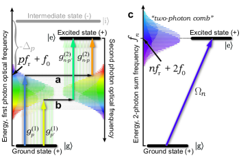
Figure 1: Constructive interference of multiple paths in a two-photon transition driven by a transform-limited optical frequency comb. All pairs of comb teeth whose sum frequency matches the excited state energy interfere constructively to excite atoms. Two example pairs are shown as a and b, and the effective two-level system that results from the sum is shown in c. Every tooth of the resulting “two-photon comb” of resonant coupling strength $\Omega$ leverages the full power of all of the optical frequency comb teeth through this massively-parallel constructive interference.

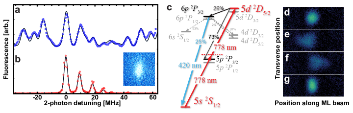
Figure 2: Laser-induced fluorescence spectrum of the $5S\!\!\rightarrow\!\!5D$ two-photon transition driven by an optical frequency comb. a: Spectrum from a natural abundance vapor cell and b: a ${}^{85}\mathrm{Rb}$ CW MOT and collected $420\mbox{ nm}$ light (inset). Solid curves are theory fitted for a Gaussian and b Voigt line shapes. c: Relevant levels of rubidium. d-g: absorption images of the atom cloud after free expansion following d: no ML illumination, e: ML illumination from the right, f: left and g: both directions, detuned to the red of resonance. Mechanical forces are evident in e and f, and the narrowing of the velocity distribution in the horizontal direction in g is the hallmark of cooling.

In contrast to CW lasers, mode-locked (ML) lasers have very high instantaneous intensity and can therefore be efficiently frequency multiplied to the UV. However, the spectrum of a ML laser consists of many evenly spaced spectral lines (an optical frequency comb) spanning a bandwidth much larger than a typical Doppler shift, and ML lasers have therefore found very little use as control tools for cooling the motion of atoms and molecules. Doppler cooling with combs has been investigated in a mode where each atom interacts with only one or two comb teeth at a time, which uses only a small fraction of the laser’s total power Strohmeier et al. (1989); Watanabe et al. (1996); Ilinova et al. (2011); Aumiler and Ban (2012); Davila-Rodriguez et al. (2016). Here, following the observation of a pushing force by Marian et al. Marian et al. (2004) and a proposal by Kielpinski Kielpinski (2006), we utilize a coherent effect in far-detuned ML two-photon transitions Baklanov and Chebotayev (1977) to laser cool atoms with all of the comb teeth contributing in parallel to enhance the scattering rate (Fig. 1). This technique is designed to allow us to utilize the high UV conversion efficiency of ML lasers without wasting any of the resulting UV power, and opens the door to laser cool H, C, N, O, and anti-hydrogen ($\bar{\mbox{H}}$), species for which single-photon laser cooling is beyond the reach of even ML lasers Kielpinski (2006). We extend these ideas to create a magneto-optical trap, and find that the density of the comb spectrum introduces no measurable effects in our system, demonstrating that it may be possible to create MOTs of these species using this technique.

A simple model can be used to describe the interaction between three-level atoms and an optical frequency comb for two-photon laser cooling and trapping (see Fig. 1 and Methods for details). The two-photon coupling strength between the ground and excited states in this case will also be a comb (the “two-photon comb” shown in Fig. 1c), the $n^{\mathrm{th}}$ tooth of which is associated with a frequency $f_{n}=nf_{\mathrm{r}}+2f_{0}$, where $f_{0}$ is the carrier-envelope offset frequency of the optical comb and $f_{\mathrm{r}}\equiv 1/T_{\mathrm{r}}$ is the pulse repetition rate. For a transform-limited ML laser, we can model the effective (time-averaged) resonant Rabi frequency of the $n^{\mathrm{th}}$ tooth of this two-photon comb as

$$\Omega_{n}=\sum_{p}\frac{g^{(1)}_{p}g^{(2)}_{n-p}}{2\Delta_{p}}$$ (1)

where $g^{(1)}_{p}$ is the resonant single-photon Rabi frequency for excitation from the ground ${\left|{\mathrm{g}}\right\rangle}$ to the intermediate state ${\left|{\mathrm{i}}\right\rangle}$ due to the $p^{\mathrm{th}}$ optical comb tooth and $g^{(2)}_{p}$ is the same quantity for excitation from the intermediate state ${\left|{\mathrm{i}}\right\rangle}$ to the excited state ${\left|{\mathrm{e}}\right\rangle}$ (Fig. 1a,b). The single-photon detuning from the intermediate state is $\Delta_{p}=pf_{\mathrm{r}}+f_{0}-f_{\mathrm{gi}}$ where $f_{\mathrm{gi}}$ is the intermediate state’s energy divided by Planck’s constant $h$ (we take the energy of the ground state to be zero). If we denote by $N$ the index of the two-photon comb tooth closest to resonance (associated with the optical sum frequency $f_{N}=Nf_{\mathrm{r}}+2f_{0}$) and the pulse duration is short compared to the excited state’s lifetime ($\tau\equiv 1/\gamma$), we can approximate the resonant Rabi frequency of each two-photon comb tooth in the vicinity of resonance as being given by $\Omega_{N}$. In the limit of weak single-pulse excitation ($\Omega_{N}T_{\mathrm{r}}\ll\pi$), the time-averaged excitation rate for an atom moving with velocity $v$ is given by (see Ref.  Ilinova et al. (2011); Aumiler and Ban (2012) and Methods)

$$\gamma_{\mathrm{comb}}=\frac{\Omega_{N}^{2}T_{\mathrm{r}}}{4}\frac{\mathrm{sinh}\!\left(\gamma\,T_{\mathrm{r}}/2\right)}{\mathrm{cosh}\!\left(\gamma\,T_{\mathrm{r}}/2\right)-\cos\!\left(\delta_{N}(\mbox{\boldmath$v$})\,T_{\mathrm{r}}\right)}$$ (2)

where $\delta_{N}(\mbox{\boldmath$v$})\equiv 2\pi(f_{N}-f_{\mathrm{ge}}-f_{N}\mbox{\boldmath$\hat{k}$}\cdot\mbox{\boldmath$v$}/c)$ is the detuning of the $N^{\mathrm{th}}$ two-photon comb tooth from two-photon resonance, $\hat{k}\mbox{ }$is a unit vector pointing in the direction of laser propagation, and $f_{\mathrm{ge}}$ is the energy of the excited state divided by $h$. If both the detuning $\delta_{N}(\mbox{\boldmath$v$})$ and natural linewidth $\gamma$ are small compared to the comb tooth spacing ($2\pi f_{\mathrm{r}}$), this two-photon comb can be treated as having only a single tooth (monochromatic interaction) with a two-photon Rabi frequency of $\Omega_{N}$. Most of the work we describe here takes place once the atoms are fairly cold ($kv\ll 2\pi f_{\mathrm{r}}$) in this “single two-photon tooth limit,” which gives rise to an excitation rate of

$$\gamma_{N}=\frac{\Omega_{N}^{2}}{\gamma}\frac{1}{1+\left(2\delta_{N}(\mbox{\boldmath$v$})/\gamma\right)^{2}}.$$ (3)

Since the AC Stark shifts from the proximity of the intermediate state to the optical photon energy are the same order of magnitude as $\Omega_{N}$, they can be neglected compared to the linewidth in the low-saturation limit. For cases where a single laser photon has enough energy to photoionize an excited atom, since both the time-averaged excitation rate and the time-averaged photoionization rate from the excited state depend only upon the time-averaged intensity, the average ionization rate is exactly the same as for a CW laser with the same frequency and time-averaged power Kielpinski (2006).

Using this simplification, an algebraic model for Doppler cooling can be constructed for the degenerate two-photon case (as opposed to two-color excitation Wu et al. (2009)) to estimate the Doppler temperature. We assume that the laser’s center frequency is near $f_{\mathrm{ge}}/2$ and that the single tooth of interest in the two-photon comb can be characterized by a two-photon saturation parameter $s_{N}\!\equiv\!2\Omega_{N}^{2}/\gamma^{2}\!\ll\!1$. For slow atoms ($kv\!\ll\!\gamma$), the cooling power of a 1D, two-photon optical molasses detuned $\gamma/2$ to the red side of two-photon resonance is given by the same expression as the single-photon CW laser cooling case, $\partial E/\partial t|_{\mathrm{cool}}=-s_{N}\hbar\omega_{\mathrm{ge}}^{2}v^{2}/c^{2}$, where $\omega_{\mathrm{ge}}\equiv 2\pi f_{\mathrm{ge}}$. The heating caused by momentum kicks from absorption is likewise identical to the CW single-photon expression, $\partial E/\partial t|_{\mathrm{heat,abs.}}=s_{N}\gamma\hbar^{2}\omega_{\mathrm{ge}}^{2}/4mc^{2}$.

The heating caused by spontaneous emission, however, is modified by both the multi-photon nature of the emission and the details of excitation by a comb as follows. First, the decay of the excited state is likely to take place in multiple steps due to the parity selection rule, splitting the de-excitation into smaller momentum kicks that are unlikely to occur in the same direction, reducing the heating. Second, two-photon laser cooling with counter-propagating CW laser beams adds heating in the form of Doppler-free (two-beam) excitations Zehnlé and Garreau (2001), which produce no cooling force in 1D but do cause heating through the subsequent spontaneous emission. By using a comb, however, one can easily eliminate these Doppler-free transitions through timing by ensuring that pulses propagating in different directions do not hit the atoms simultaneously. In the frequency domain, this delay produces a frequency-dependent phase shift of the frequency comb for the second photon (shown on the right side of Fig. 1a, b), destroying the coherent addition of comb teeth pairs necessary to drive the transition. The net result is that the heating rate from spontaneous emission for two-photon laser cooling with an optical frequency comb can be modeled by

$$\left.\frac{\partial E}{\partial t}\right|_{\mathrm{heat,spon.}}=s_{N}\gamma\frac{\hbar^{2}\omega_{\mathrm{ge}}^{2}}{8mc^{2}}.$$ (4)

The balance between the cooling power and the sum of these heating powers occurs at the Doppler temperature for two-photon laser cooling with an optical frequency comb:

$$T_{\mathrm{D}}=\frac{3}{4}\frac{\hbar\gamma}{2k_{\mathrm{B}}}$$ (5)

where $k_{\mathrm{B}}$ is the Boltzmann constant.

As a first experimental test of direct frequency comb 2-photon cooling and trapping, we report a demonstration of the technique using rubidium atoms. For the $5{}^{2}S_{1/2}\!\!\rightarrow\!\!5{}^{2}D_{5/2}$ transition in rubidium, the natural decay rate of the excited state is $\gamma/2\pi=667\mbox{ kHz}$ Sheng et al. (2008). Eq. (5) gives a Doppler cooling limit of $12\mbox{ }\mu\mbox{K}$, which will also be true in 3D for a ML laser with non-colliding pulses. In this work, we apply cooling in 1D with spontaneous emission into 3D, and our effective transition linewidth must also be taken into account (see Methods), which yields a predicted Doppler limit of $31\mbox{ }\mu\mbox{K}$ for this system, considerably colder than the single-photon $5{}^{2}S_{1/2}\!\rightarrow\!5{}^{2}P_{3/2}$ 3D Doppler limit of $146\mbox{ }\mu\mbox{K}$.

The optical frequency comb in this work is generated from a Ti:Sapphire laser emitting $2\!\!-\!\!5\mbox{ ps}$ pulses (less than $500\mbox{ GHz}$ bandwidth) at $778\mbox{ nm}$ at a repetition rate of $f_{\mathrm{r}}=81.14\mbox{ MHz}$.

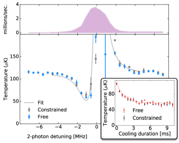
Figure 3: Detuning dependence of $420\mbox{ nm}$ fluorescence (top) and the resulting temperature (bottom) of rubidium atoms laser-cooled by an optical frequency comb on a two-photon transition. The solid curve is fit for scattering rate, effective linewidth and detuning offset of data analyzed with the aid of a monte carlo technique (data labeled “Constrained,” see Methods). The same data are also analyzed using a free expansion model (“Free”), and agree well with the monte carlo assisted analysis. (Inset) temperature vs. time when the laser detuning is optimized for cooling, giving a minimum temperature of $(57\pm 2)\mbox{ }\mu\mbox{K}$. Error bars are statistical over repeated measurements.

We prepare an initial sample of $\approx 10^{7}$ ${}^{85}\mathrm{Rb}$ atoms using a standard CW laser MOT at $780\mbox{ nm}$. The magnetic field and the CW laser cooling light are then turned off, leaving the atoms at a temperature typically near $110\mbox{ }\mu\mbox{K}$. A weak CW “repump” laser is left on continuously to optically pump atoms out of the $F_{\mathrm{g}}=2$ ground state, and has no measurable direct mechanical effect. Each ML beam typically has a time-averaged power of $(500\pm 50)\mbox{ mW}$ and a diameter of $(1.1\pm 0.1)\mbox{ mm}$. After illumination by the ML laser, the atoms are allowed to freely expand and are subsequently imaged using resonant CW absorption to determine their position and velocity distributions.

By monitoring the momentum transfer from a single ML beam (Fig. 2e, f), we measure a resonant excitation rate to be $\gamma_{\mathrm{scatt}}=(6500\pm 700)\mbox{ s}^{-1}$. Our theoretical estimate from Eq. (1) and our laser parameters gives $(13000\pm 2000)\mbox{ s}^{-1}$, which suggests that there may be residual chirp in the pulses that is suppressing the excitation rate by about a factor of 2. The measured rate is well above the threshold needed to support these atoms against gravity ($\approx 810\mbox{ s}^{-1}$), which suggests that 3D trapping should be possible with additional laser power for the inclusion of four more beams.

We observe Doppler cooling and its dependence on two-photon detuning by applying counter-propagating linearly-polarized ML beams to the atom cloud for $4\mbox{ ms}$ in zero magnetic field. By fitting the spatial distribution of the atoms (see Methods), we extract a 1D temperature, shown in Fig. 3. The solid curve is based on the algebraic model used above to derive the Doppler limit and is fit for a resonant single-beam excitation rate of $(4800\pm 400)\mbox{ s}^{-1}$ and linewidth $\gamma_{\mathrm{eff}}/2\pi=(1.88\pm 0.07)\mbox{ MHz}$, consistent with the single-beam recoil measurements. We realize a minimum temperature of $(57\pm 2)\mbox{ }\mu\mbox{K}$ (Fig. 3, inset). However, the reduced temperature is hotter than the expected Doppler limit of $31\mbox{ }\mu\mbox{K}$ for our system (see Methods). We find experimentally that the temperature inferred from free-expansion imaging is highly sensitive to beam alignment, and therefore suspect the discrepancy is due to imperfect balancing of the forward and backward scattering forces at some locations in the sample Lett et al. (1989).

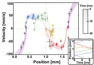
Figure 4: Phase space (and position space, inset) trajectories for atoms trapped in a two-photon, optical frequency comb MOT. Smooth curves are fits to a damped harmonic oscillator, with fit uncertainties shown as bands. Purple features show the behavior when the ML beam polarizations are intentionally reversed and exhibit an anti-confining force. Error bars are statistical over repeated measurements.

To investigate the feasibility of using this technique to make a MOT, a quadrupole magnetic field with a gradient of $7.7\mbox{ G}/\mbox{cm}$ is introduced and the ML beam polarizations are set to drive $\sigma^{\pm}$ transitions in the standard single-photon CW MOT configuration Raab et al. (1987). We displace the atom cloud from the trap center and monitor the atoms as they are pushed toward the trap center, as shown in Fig. 4. The system is modeled as a damped harmonic oscillator and fitting the motion of the atoms yields a trapping frequency of $\nu_{\mathrm{MOT}}=(40\pm 9)\mbox{ Hz}$ and a cyclic damping rate of $(37\pm 4)\mbox{ Hz}$. These MOT parameters imply a resonant excitation rate of $(7000\pm 1000)\mbox{ s}^{-1}$ and an effective magnetic line shift of $(0.5\pm 0.2)\mbox{ }\mu_{\mathrm{B}}$. The average of the calculated line shifts for all $\Delta m_{F}=+2$ transitions would be $1.2\mbox{ }\mu_{\mathrm{B}}$ for $F_{\mathrm{g}}=3\!\!\rightarrow\!\!F_{\mathrm{e}}=5$, suggesting that some $\pi$-polarization may be playing a role. We are unable to detect any measurable atom loss in the few milliseconds of ML illumination before atoms exit the interaction volume due to transverse motion, consistent with the measured photoionization cross section Duncan et al. (2001).

This demonstration with rubidium shows that it may be possible to apply these techniques in the deep UV to laser cool and magneto-optically trap species such as H, C, N, O, and $\bar{\mbox{H}}$ (anti-hydrogen). Due to low anticipated scattering rates, these species will likely need to be slowed using other means Hogan et al. (2008); Hummon et al. (2008). Direct comb laser cooling and trapping would then be used to cool them to the Doppler limit in a MOT.

For H and $\bar{\mbox{H}}$, to minimize photoionization losses (of particular importance for $\bar{\mbox{H}}$, see Methods), we propose two-photon cooling on $1S\!\!\rightarrow\!\!3D$ at $205.0\mbox{ nm}$. By choosing a comb tooth spacing of $f_{\mathrm{r}}=83.5\mbox{ MHz}$, all six of the allowed hyperfine and fine structure transitions on $1S\!\!\rightarrow\!\!3D$ can be driven simultaneously with a red detuning between $\gamma/3$ and $\gamma$. We estimate a resonant excitation rate on $1S\!\!\rightarrow\!\!3D$ of $\gamma_{\mathrm{scatt}}\approx 1250\mbox{ s}^{-1}$ is achievable with demonstrated technology (see Methods). This excitation rate would produce an acceleration more than 50 times greater than that used in this work to make a MOT of rubidium.

Atomic oxygen has fine structure in its ${{}^{3}}P$ ground state that spans a range of about $7\mbox{ THz}$, so the comb’s ability to drive multiple transitions at once is a crucial advantage. For the $(2p^{4}){}^{3}P\!\!\rightarrow\!\!(3p){}^{3}P$ transitions, a frequency comb centered at $226\mbox{ nm}$ with a $2\mbox{ nm}$ bandwidth would be able to drive simultaneous 2-photon transitions for each fine structure component for a repetition rate near $79.79\mbox{ MHz}$. Nitrogen cooling and trapping would proceed on the $(2p^{3}){}^{4}S_{3/2}^{o}\!\!\rightarrow\!\!(3p){}^{4}S_{3/2}^{o}$ two-photon transition at $207\mbox{ nm}$. Branching to the doublet manifold limits the total number of quartet excitations per atom to $\approx 10^{3}$, sufficient for laser cooling a hot, trapped sample Hummon et al. (2008) to the Doppler limit. The hyperfine structure in the ground state of ${}^{15}N$ is split by $29\mbox{ MHz}$, so excitation from a single two-photon tooth may be enough to produce both cooling and (off-resonant) hyperfine repumping. Carbon would likely require multiple combs Kielpinski (2006), but each would operate on the same principles we have investigated here.

This demonstration with rubidium confirms the essential aspects of laser cooling and trapping with frequency combs on 2-photon transitions. Future work in extending this technique into the deep UV should be possible with the addition of frequency conversion stages for the ML light. In particular, as higher power UV frequency combs become available Kanai et al. (2009); Pronin et al. (2015), the technology for laser cooling and trapping will extend the reach of these techniques to species that cannot currently be produced in ultracold form.

I methods

I.1 Frequency lock for the optical frequency comb

To tune the ML laser near the resonance condition for the $5S\!\!\rightarrow\!\!5D$ two-photon transition in rubidium (Fig. 2), we sample a fraction of the laser power and send it to a hot Rb vapor cell in a counter-propagating geometry Reinhardt et al. (2010). Each excitation to the $5{}^{2}D_{5/2}$ state produces a spontaneously emitted $420\mbox{ nm}$ photon as part of a cascade decay 6.5% of the time (Fig. 2c), which is collected from the pulse collision volume and monitored with a photon-counting detector. Fig. 2a shows the resulting Doppler-free spectrum of the 32 allowed two-photon transitions for both ${}^{85}\mathrm{Rb}$ and ${}^{87}\mathrm{Rb}$ from the $5S$ to $5D$ manifolds. Since the bandwidth of the comb ($<500\mbox{ GHz}$) is smaller than the detuning from 1-photon resonance with the $5P$ states ($\Delta/2\pi>1\mbox{ THz}$), the spectrum repeats itself with a (two-photon sum frequency) period of $f_{\mathrm{r}}$. We laser cool and trap ${}^{85}\mathrm{Rb}$ using the $5{}^{2}S_{1/2},F_{\mathrm{g}}=3$ to $5{}^{2}D_{5/2},F_{\mathrm{e}}=5$ “stretch” transition.

To maintain sufficient laser stability for Doppler cooling and trapping, we stabilize the ML laser by locking it to an external cavity. The free spectral range of the external cavity is pressure tuned to be an integer multiple ($q=25$) of the ML laser repetition rate to guarantee that multiple teeth from across the laser spectrum contribute to the Pound-Drever-Hall error signal used for the lock. A piezo-mounted mirror on the external cavity is then used to stabilize it to the $5{}^{2}S_{1/2},F_{\mathrm{g}}=3$ to $5{}^{2}D_{5/2},F_{\mathrm{e}}=5$ line using FM spectroscopy of the vapor cell. We note that this optical frequency comb is not self referenced and that we feed back to an unknown combination of $f_{\mathrm{r}}$ and $f_{0}$ to maintain the two-photon resonance condition, which is the only frequency parameter that needs to be actively stabilized. The pulse chirp is periodically minimized by adjusting a Gires-Tournois interferometer in the laser cavity to maximize the blue light emitted from atoms in the initial CW MOT. The frequency of the ML laser light used for cooling and trapping is tuned from the vapor cell lock point using an acousto-optic modulator downstream.

I.2 Effective two-photon Rabi frequency

We model the electric field of a frequency comb propagating along +$z$ in the plane wave approximation as

$$\mathbf{E}(z,t) = \frac{\mathcal{E}_{\mathrm{o}}}{2}\mathrm{Env}(t)\sum_{q}h(t\!-\!qT_{\mathrm{r}})\left(\mbox{\boldmath{$\hat{\epsilon}$}}\,e^{-i(2\pi f_{\mathrm{c}}(t-qT_{\mathrm{r}})+q2\pi f_{0}T_{\mathrm{r}}-kz)}\right.$$ (6)

$$\left.\;\;\;\;\;\;\;\;\;\;\;+\,\mbox{\boldmath{$\hat{\epsilon}$}}^{\ast}e^{i(2\pi f_{\mathrm{c}}(t-qT_{\mathrm{r}})+q2\pi f_{0}T_{\mathrm{r}}-kz)}\right)$$

where $\mathrm{Env}(t)$ is the slowly-varying envelope of the pulse train (we will take this to be equal to 1), $\mathcal{E}_{\mathrm{o}}h(0)$ is the peak instantaneous electric field amplitude, $h(t)$ is the envelope of a single pulse (peaked at $t=0$), $\hat{\epsilon}$ is the unit vector describing the laser polarization, $f_{\mathrm{c}}$ is the carrier frequency of the laser and $f_{0}$ is the carrier-envelope offset frequency. If the pulse envelope $h(t)$ is real and symmetric about $t=0$ with Fourier transform $\tilde{\mathrm{H}}(\omega)$, we can rewrite Eq. (6) as

$$\mathbf{E}(z,t)=\sum_{p}\frac{\mathcal{E}_{p}}{2}\left(\mbox{\boldmath{$\hat{\epsilon}$}}e^{-i(2\pi f_{p}t-kz)}+\mbox{\boldmath{$\hat{\epsilon}$}}^{\ast}e^{i(2\pi f_{p}t-kz)}\right)$$ (7)

where $f_{p}\equiv pf_{\mathrm{r}}+f_{0}$ is the cyclic frequency of the $p^{\mathrm{th}}$ optical frequency comb tooth and

$$\mathcal{E}_{p}=\mathcal{E}_{\mathrm{o}}\frac{\tilde{\mathrm{H}}(2\pi(f_{p}-f_{\mathrm{c}}))}{T_{\mathrm{r}}}$$ (8)

is the time-averaged electric field amplitude of the $p^{\mathrm{th}}$ optical frequency comb tooth. The single-photon resonant Rabi frequency for just the $p^{\mathrm{th}}$ tooth to drive the $\mathrm{g}\!\rightarrow\!\mathrm{i}$ transition is given by

$$g_{p}^{(\mathrm{gi})}=\frac{e\mathcal{E}_{p}}{\hbar}{\left\langle{\mathrm{i}}\right|}\mbox{\boldmath{$\hat{\epsilon}$}}\cdot\mathbf{r}{\left|{\mathrm{g}}\right\rangle}$$ (9)

(where $\mathbf{r}$ is the position operator for the electron) and likewise for $\mathrm{i}\!\rightarrow\!\mathrm{e}$, which appear in Eq. (1) as $g^{(1)}$ and $g^{(2)}$, respectively.

The $5{}^{2}S_{1/2}\!\!\rightarrow\!\!5{}^{2}D_{5/2}$ two-photon transition near $778\mbox{ nm}$ in rubidium primarily gets its strength through single-photon couplings to the nearby $5{}^{2}P_{3/2}$ state, which approximation was made implicitly in Eq. (1). For the more general case, the $\mathrm{g}\!\!\rightarrow\!\!\mathrm{e}$ two-photon Rabi frequency includes a sum over all of the possible intermediate states $\{{\left|{\mathrm{i}}\right\rangle}\}$. Matrix elements for calculating AC Stark shifts and photoionization are similar, but include single photon detunings $\Delta$ for both emission first and absorption first. In the case of hydrogen, it is even important to include continuum states in the sum over $\mathrm{i}$, which contribute substantially Haas et al. (2006). The two-photon resonant Rabi frequency associated with the $n^{\mathrm{th}}$ tooth of the “two-photon” comb can be written

$$\Omega_{n}=\sum_{p}\frac{e^{2}\mathcal{E}_{p}\mathcal{E}_{n-p}}{\hbar^{2}}{\left\langle{\mathrm{e}}\right|}(\mbox{\boldmath{$\hat{\epsilon}$}}\cdot\mathbf{r})\left(\sum_{\mathrm{i}}\frac{{\left|{\mathrm{i}}\right\rangle\!\!\left\langle{\mathrm{i}}\right|}}{2\Delta_{p}^{(\mathrm{i})}}\right)(\mbox{\boldmath{$\hat{\epsilon}$}}\cdot\mathbf{r}){\left|{\mathrm{g}}\right\rangle}.$$ (10)

For a comb whose spectrum is centered approximately halfway between ${\left|{\mathrm{e}}\right\rangle}$ and ${\left|{\mathrm{g}}\right\rangle}$, the time-averaged laser intensity $I$ is related to this via $\sum_{p}\mathcal{E}_{p}\mathcal{E}_{n-p}\approx 2I/\epsilon_{\mathrm{o}}c$.

In the limit that all of the single-photon detunings $\Delta_{p}^{(\mathrm{i})}$ are much larger than the fine and hyperfine splittings (which is often valid, but is not applicable for the $778\mbox{ nm}$ line in rubidium), since the term in parentheses includes a sum over all possible projection quantum numbers, it is rotationally invariant and the angular momentum prefactors for calculating $\Omega_{n}$ arise entirely from the tensor $(\mbox{\boldmath{$\hat{\epsilon}$}}\cdot\mathbf{r})(\mbox{\boldmath{$\hat{\epsilon}$}}\cdot\mathbf{r})$. This limit holds well for hydrogen, and the tensor products can be used to calculate direct two-photon matrix elements between single quantum states by using the Wigner-Eckhart theorem and a single reduced matrix element Haas et al. (2006). Each irreducible spherical tensor component contained in $(\mbox{\boldmath{$\hat{\epsilon}$}}\cdot\mathbf{r})(\mbox{\boldmath{$\hat{\epsilon}$}}\cdot\mathbf{r})$ can be factored into the product of a polarization-independent term that contracts $\mathbf{r}$ with itself and an atom-independent term that depends only on the polarization, $\mathrm{T}^{(k)}[\mbox{\boldmath{$\hat{\epsilon}$}},\mbox{\boldmath{$\hat{\epsilon}$}}]$, which is known as the polarization tensor Zare (1988). The rank 0 tensor product $\mathrm{T}^{(0)}[\mathbf{r},\mathbf{r}]$ is responsible for ${}^{2}S_{1/2}\!\!\rightarrow\!\!{}^{2}S_{1/2}$ transitions, while the rank 2 tensor $\mathrm{T}^{(2)}[\mathbf{r},\mathbf{r}]$ gives rise to the $S\!\!\rightarrow\!\!D$ transition amplitude in analogy to an electric quadrupole interacting with an electric field gradient. Reduced matrix elements for two-photon transitions and ionization rates in hydrogen have been calculated by Haas et al. Haas et al. (2006) for linearly polarized light, and therefore include the value of the polarization tensor for linear ($\mbox{\boldmath{$\hat{\epsilon}$}}=\hat{\mathbf{z}}$) polarization $\mathrm{T}^{(k)}[\hat{\mathbf{z}},\hat{\mathbf{z}}]$.

In order to use these reduced matrix elements for the case of $\sigma^{+}$ or $\sigma^{-}$ light, they need to be scaled to reflect the change of the polarization tensor. This scaling factor is the term responsible for the increased strength of the $\sigma^{+}$ or $\sigma^{-}$ transitions as compared to $\pi$ polarizations. For $1S\!\!\rightarrow\!\!3D$, there is a convenient comb repetition rate ($f_{\mathrm{r}}=83.5\mbox{ MHz}$, see Fig. 5) such that all of the possible fine and hyperfine transitions of $1S\!\!\rightarrow\!\!3D$ can be driven simultaneously. For a single $\sigma^{+}$ (or $\sigma^{-}$) polarized comb on two-photon resonance for $1S\!\!\rightarrow\!\!3D$ stretch transitions with unresolved fine and hyperfine structure, we use the reduced matrix element $\beta_{ge}^{(2)}$ of Ref. Haas et al. (2006) times the ratio of the circular to linear rank 2 polarization tensor components ($=\sqrt{6}/2$) to calculate the two-photon resonant Rabi frequency,

$$\Omega/2\pi=-6.8\,I\times 10^{-5}\mbox{ Hz}(\mbox{W/m}^{2})^{-1}.$$ (11)

Likewise, the ionization rate is given by the ionization rate for the $3D$ state times the fraction of atoms that are in the $3D$ state ($\approx\Omega^{2}/\gamma^{2}$):

$$\gamma_{\mathrm{ionization}}/2\pi=I\frac{\Omega^{2}}{\gamma^{2}}\,1.9\times 10^{-6}\mbox{ Hz}(\mbox{W/m}^{2})^{-1}$$ (12)

where $\gamma/2\pi=10.3\mbox{ MHz}$ is the $3D$ state decay rate and we have used the reduced matrix elements provided by Ref.  Haas et al. (2006) rescaled to reflect the value of $\mathrm{T}^{(2)}_{0}[\mbox{\boldmath{$\hat{\epsilon}$}},\mbox{\boldmath{$\hat{\epsilon}$}}^{\ast}]/\mathrm{T}^{(2)}_{0}[\hat{\mathbf{z}},\hat{\mathbf{z}}]=-1/2$.

I.3 Scattering rate from a frequency comb

To estimate the scattering rate from a frequency comb of coupling strength $\Omega$ between a ground and excited state (whether it is due to a single or multi-photon process), we define the resonant saturation parameter for the $n^{\mathrm{th}}$ comb tooth to be $s_{n}\equiv 2\Omega_{n}^{2}/\gamma^{2}$, where $\gamma$ is the decay rate of the excited state, which we will model as decaying only to the ground state. We focus on the limit where $s_{n}\ll 1$ and $\Omega_{n}T_{\mathrm{r}}\ll\pi$ due to the low Rabi frequency expected for two-photon transitions under realistic experimental conditions. For optical forces, we are typically most interested in the time-averaged scattering rate, which permits us to simplify the model by summing up the scattering rates due to each comb tooth instead of the excitation amplitudes. Specifically, the steady-state time-averaged scattering rate from the $n^{\mathrm{th}}$ comb tooth by a stationary atom will be given by

$$\gamma_{n}\approx\gamma\frac{s_{n}}{2}\frac{1}{1+(2\delta_{n}/\gamma)^{2}}$$ (13)

where $\delta_{n}\equiv 2\pi(f_{n}-f_{\mathrm{ge}})$ is the detuning of the $n^{\mathrm{th}}$ comb tooth from resonance. If the center frequency of the comb of coupling strength is near $f_{\mathrm{ge}}$ and the pulse duration is short compared to the excited state lifetime, $s_{n}$ will change very little over the range of $n$ that is within a few $\gamma$ of resonance and we can approximate $s_{n}=s_{N}$ where $N$ is the index of the comb tooth closest to resonance. In this case, we can use the identity

$$\sum_{n=-\infty}^{\infty}\frac{1}{1+a^{2}(n-b)^{2}}=\frac{\pi}{a}\frac{\mathrm{sinh}\!\left(2\pi/a\right)}{\mathrm{cosh}\!\left(2\pi/a\right)-\cos(2\pi b)}$$ (14)

to write

$$\gamma_{\mathrm{comb}}=\sum_{n}\gamma_{n}=\gamma\frac{s_{N}}{2}\frac{(\gamma\,T_{\mathrm{r}}/4)\,\mathrm{sinh}\!\left(\gamma\,T_{\mathrm{r}}/2\right)}{\mathrm{cosh}\!\left(\gamma\,T_{\mathrm{r}}/2\right)-\cos(\delta_{N}T_{\mathrm{r}})}.$$ (15)

In the limit where both $\delta_{N}/2\pi$ and $\gamma/2\pi$ are small compared to the repetition rate $f_{\mathrm{r}}$, Eq. (15) reduces to Eq. (13) with $\gamma_{\mathrm{comb}}\approx\gamma_{N}$. For the laser cooling and trapping we report with rubidium, the combined effect of all of the off-resonant comb teeth to the scattering rate when $\delta_{N}=-\gamma/2$ is approximately $10^{-4}\gamma_{N}$, and we can neglect their presence for slow-moving atoms. For hydrogen laser cooling on $1S\!\!\rightarrow\!\!3D$ at $f_{\mathrm{r}}=83.5\mbox{ MHz}$, this fraction is less than 0.04, and the single-tooth approximation is likely to be fair.

I.4 Estimates for application to hydrogen, nitrogen, and oxygen

For H and $\bar{\mbox{H}}$, two-photon Doppler cooling has previously been proposed on the $1S\!\!\rightarrow\!\!2S$ transition (through forced quenching of the $2S$ state) with a CW laser Zehnlé and Garreau (2001) or optical frequency comb Kielpinski (2006) centered at $243\mbox{ nm}$. Photoionization from the $2S$ state sets a limit on the intensity and effective (quenched) linewidth for this scheme, which ultimately limits the scattering rate. The photoionization cross section of the $3D$ state is approximately two orders of magnitude smaller than the $2S$ state for photons at half the state energy Haas et al. (2006). We therefore estimate parameters here for two-photon cooling on $1S\!\!\rightarrow\!\!3D$ at $205.0\mbox{ nm}$, which is within the phase matching window for production by frequency doubling in BBO. We propose that the added difficulty of producing light at this deeper UV wavelength is justified by the lower photoionization rate and is further mitigated by the fact that for this transition, multiple teeth of the two-photon comb (Eq. (1) and Fig. 1c) can be used simultaneously to drive different hyperfine and fine-structure transitions in parallel at no cost in additional laser power ( Fig. 5). In the limit that both the average and instantaneous excited state probabilities are small ($\Omega_{N}\ll\gamma<2\pi f_{\mathrm{r}}$) with unequal detunings from resonance for each transition being driven, coherences between multiple excited states can be neglected and each line will act essentially as an independent two-level system.

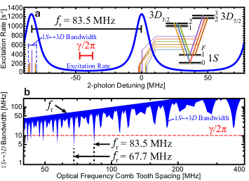
Figure 5: Calculated parameters for laser cooling atomic hydrogen on $1S\!\!\rightarrow\!\!3D$. a Calculated excitation rate (blue) as a function of twice the optical frequency (the two-photon effective frequency at $102.5\mbox{ nm}$) for a comb with repetition rate $f_{\mathrm{r}}=83.5\mbox{ MHz}$. The spectrum shown is the atomic spectrum modulo $f_{\mathrm{r}}$, which is how the spectrum will appear when scanning a frequency comb. b The bandwidth spanned by the six allowed fine and hyperfine transition frequencies $\mathrm{mod}f_{\mathrm{r}}$ is less than the natural linewidth of $\gamma/2\pi=10.3\mbox{ MHz}$ for this repetition rate and a few others.

In Fig. 5, it is shown that that by choosing a comb tooth spacing of $f_{\mathrm{r}}=83.5\mbox{ MHz}$, all six of the allowed Bonin and McIlrath (1984) hyperfine and fine structure transitions Kramida (2010) on $1S\!\!\rightarrow\!\!3D$ can be driven simultaneously with a red detuning between $\gamma/3$ and $\gamma$. This illustrates the optical frequency comb’s ability to act as its own hyperfine “repump,” and allows this scheme to be applied robustly to magnetically trapped samples, where the presence of polarization imperfections or off-resonant excitation to undesired excited states can cause spin flips that must be repumped. Though not the focus of this work with two-photon transitions, we have verified experimentally that we can load and trap rubidium atoms in a one-photon optical frequency comb MOT that accomplishes its own hyperfine repumping with another tooth through judicious choice of the repetition rate.

Optical frequency combs at $205\mbox{ nm}$ with $\approx 100\mbox{ mW}$ of time-averaged power and build-up cavity power enhancement factors of up to 10 have been demonstrated Wall et al. (2003); Zhang et al. (2009); Peters et al. (2009, 2013). Focusing the intra-cavity $1\mbox{ W}$ beam to a spot size with diameter $60\mbox{ }\mu\mbox{m}$ to make a 1D optical molasses would produce a resonant excitation rate on $1S\!\!\rightarrow\!\!3D$ that is shown as a function of frequency in Fig. 5a. The photoionization rate at the peak scattering frequency would be $\gamma_{\mathrm{ionization}}<0.2\mbox{ s}^{-1}$ under these circumstances, so each atom would be able to scatter thousands of photons before being ionized.

I.5 Doppler limit for two-photon optical molasses

To derive the Doppler cooling limit for (approximately equal frequency) two-photon transitions, we take an algebraic approach to derive one cooling and two heating mechanisms that will balance one another in equilibrium Foot (2005). We first derive the 1D Doppler cooling limit for two-photon laser cooling with a CW laser (or a comb with pulses colliding simultaneously on the atoms), then examine the situation for an optical frequency comb where there is some finite delay time that is longer than the pulse duration between forward and backward propagating pulses. We will assume that the two-photon transitions are driven well below saturation (resonant saturation parameter $s_{N}\ll 1$) and with a two-photon detuning of $\gamma/2$ to the red side of resonance. In the case of cooling with an optical frequency comb, we will assume that the single-tooth approximation discussed above is valid.

The average cooling force is given by the product of the momentum transfer per excitation and the excitation rate. In the limit where the Doppler shifts are small compared to the excited state linewidth, the cooling power is given by $\partial E/\partial t|_{\mathrm{cool}}=-s_{N}\hbar\omega_{\mathrm{ge}}^{2}v^{2}/c^{2}$.

This cooling power is balanced by two sources of heating: heating due to randomly-distributed momentum kicks from absorption events and heating due to momentum kicks from spontaneous emission Foot (2005). For the former, there are only contributions from the single-beam processes since two-beam absorption does not induce a momentum kick for counter-propagating beams, and the heating power from absorption is given by $\partial E/\partial t|_{\mathrm{heat,abs.}}=s_{N}\gamma\hbar^{2}\omega_{\mathrm{ge}}^{2}/4mc^{2}$.

The second heating term is due to spontaneous emission and will depend upon the details of the decay channels available to the excited state. If the probability that an excited atom emits a photon with frequency $\omega_{i}$ at some point on its way to the ground state is $\mathcal{P}_{i}$, the heating from these decays can be modeled with a probability-weighted sum of the squares of the momentum kicks from these spontaneously-emitted photons, viz.

$$\left.\frac{\partial E}{\partial t}\right|_{\mathrm{heat,spon.}}=\frac{1}{2m}\gamma_{\mathrm{tot}}\sum_{i}\mathcal{P}_{i}\left(\hbar\frac{\omega_{i}}{c}\right)^{2}$$ (16)

where $\gamma_{\mathrm{tot}}$ is the total excitation rate (see e.g. Eq. (15) for the case with a single beam from an optical frequency comb) and we are for the moment modeling the spontaneous emission as being confined to 1D, which gives a Doppler limit that agrees with the 3D calculation in the standard single-photon case.

Eq. (16) shows the mechanism by which multi-photon cooling can give rise to a lower Doppler limit than single-photon cooling; by splitting the decay into smaller, uncorrelated momentum kicks, the mean square total momentum transfer (and therefore the heating) will on average be lower than for a single photon decay channel. Eq. (16) also shows that there is an additional heating mechanism for the CW case since $\gamma_{\mathrm{tot}}$ will in this circumstance include two-beam excitations that are Doppler free for counter-propagating beams Zehnlé and Garreau (2001). The excitation rate from the two-beam terms (which does not contribute to the cooling in 1D) is 4 times larger than each single-beam term, and the size of this effect for 1D two-photon laser cooling of atomic hydrogen on a quenched $1S\!\!\rightarrow\!\!2S$ transition, for example, would lead to a comb-cooled Doppler temperature that is a factor of 2 lower than the predicted CW limit Zehnlé and Garreau (2001). In order to make a quantitative estimate of the magnitude of these effects, we model the decay cascade as proceeding via a single intermediate state halfway between ${\left|{\mathrm{g}}\right\rangle}$ and ${\left|{\mathrm{e}}\right\rangle}$ ($\mathcal{P}_{i}=1$ and $\omega_{i}=\omega_{\mathrm{ge}}/2$ for $i=1,2$), which gives us

$$\left.\frac{\partial E}{\partial t}\right|_{\mathrm{heat,spon.}}=s_{N}\frac{3\gamma}{8}\frac{\hbar^{2}\omega_{\mathrm{ge}}^{2}}{mc^{2}}.$$ (17)

The equilibrium temperature at which the cooling and heating terms sum to zero for the CW case gives the Doppler limit for 2-photon 1D optical molasses with counter-propagating CW laser beams

$$T_{\mathrm{D,CW}}=\frac{5}{4}\frac{\gamma\hbar}{2k_{\mathrm{B}}}.$$ (18)

This is 25% hotter than single-photon cooling on a transition with the same linewidth, despite the fact that it includes the reduction in heating from the cascade decay.

For the mode-locked case where pulses from the two directions do not collide on the atoms at the same time, the cooling power and heating power from absorption are both the same as the CW case in 1D. However, the heating power from spontaneous emission is reduced by a factor of 3 (compare Eq. (4) and Eq. (17)) due to the absence of Doppler-free absorption, and the resulting Doppler cooling limit is given by Eq. (5), which is colder than both the CW and the single-photon cases.

We have extended this model to 3D and performed the detailed decay channel sum in Eq. (16) for the rubidium transition used in this work and find that the calculated Doppler limit of $T_{\mathrm{D,comb}}=12\mbox{ }\mu\mbox{K}$ agrees well with the prediction of Eq. (5).

I.6 Finite laser tooth linewidth

By monitoring the $420\mbox{ nm}$ fluorescence from the pre-cooled (and then released) rubidium atoms as the ML laser frequency is swept (shown at the top of Fig. 3), we obtain a line shape that is more broad than the natural linewidth of $\gamma/2\pi=667\mbox{ MHz}$ Sheng et al. (2008). The Doppler broadening expected from motion would be $630\mbox{ kHz}$ if taken alone, and the magnetic field is zeroed to a level where magnetic broadening will not contribute to the spectral width. We find that, after taking into account the natural linewidth and the expected Doppler broadening, we have a residual FWHM of the two-photon spectrum of around $1.8\mbox{ MHz}$, which we attribute to the laser. It is worth noting that using this width to infer an optical (that is, single-photon) comb tooth width or vice versa is highly dependent on the details of the broadening mechanism (see, e.g. Ryan et al. (1995)), and we therefore rely on the two-photon spectroscopy exclusively for determining our relevant effective two-photon spectral linewidth, which is model-independent. Combining this with the natural linewidth again via convolution gives us an effective two-photon spectral linewidth with a FWHM of $\gamma_{\mathrm{eff}}/2\pi=2.2\mbox{ MHz}$.

To account for the effect of finite two-photon spectral linewidth on scattering rate, we approximate the line shape as Lorentzian to adopt the model of Haslwanter et al. Haslwanter et al. (1988), which in the low-intensity limit ($s_{N}\ll 1$) gives the scattering rate

$$\gamma_{N}=\frac{\Omega_{N}^{2}}{\gamma}\frac{\gamma/\gamma_{\mathrm{eff}}}{1+\left(2\delta_{N}(\mbox{\boldmath$v$})/\gamma_{\mathrm{eff}}\right)^{2}}.$$ (19)

We can recognize this as Eq. (3) with the replacement

$$\gamma\!\rightarrow\!\gamma_{\mathrm{eff}},$$ (20)

and conclude that a first approximation of the Doppler temperature limit can be made in the case of finite spectral linewidth by applying the replacement Eq. (20) to expressions for the Doppler temperature (e.g. Eq. (5)). Using this approach for our experimental case where cooling is applied in 1D but spontaneous emission is approximated as being isotropic in 3D, we predict a Doppler limit of $T_{\mathrm{D,comb}}=31\mbox{ }\mu\mbox{K}$.

I.7 Fitting absorption images for temperature

The spatial width of an atomic cloud following Maxwell-Boltzmann statistics as a function of time, $t$, is

$$w(t)=\sqrt{w_{0}^{2}+\frac{k_{\mathrm{B}}T}{m}t^{2}}$$ (21)

where $w_{0}$ is the width at $t=0$ when positions and velocities are uncorrelated. In Fig. 3 the temperature for data points labeled as “Free” are derived from fitting the free expansion to Eq. (21) where $t=0$ is defined as the end of CW laser cooling.

For the experiments shown in Fig. 3, however, we illuminate the atoms with the ML laser at times $t>0$ which introduces a damping force. The simple model of Eq. (21) does not account for the extra dynamics resulting from optical forces. We therefore developed a simulation to model an expanding cloud of atoms (in three dimensions) that is subject to the optical forces of counterpropogating laser beams in one dimension. The data points marked “Constrained” in Fig. 3 are derived from analysis that relies on our simulation. For each temperature data point we input experiment parameters (detuning, initial sample temperature, initial sample width, ML cooling duration, etc.) along with the experimental measured widths of our atomic cloud during free expansion. We run the simulation multiple times as a function of scattering rate and select the simulation that minimizes $\chi^{2}$ between the experimentally measured widths and the simulation widths. From the best simulation we define a temperature using $T=\frac{m}{k_{\mathrm{B}}}\sigma_{v}^{2}$ where $\sigma_{v}$ is the standard deviation of the simulation’s velocity distribution. Despite the fact that the free expansion model does not include effects of the ML laser, the two methods give almost the same temperatures, which can be seen by comparing the blue and gray points in Fig. 3 and the black and red points in the inset of that figure. There seems to be a slightly higher inferred temperature when the monte carlo assisted analysis (“Constrained”) is used in cases where the acceleration from the ML laser is large.