Approximate Analytic Solutions to Coupled Nonlinear Dirac Equations
Avinash Khare
khare@physics.unipune.ac.inPhysics Department, Savitribai Phule Pune University, Pune 411007, India
Fred Cooper
cooper@santafe.eduSanta Fe Institute, Santa Fe, NM 87501, USA
Theoretical Division and Center for Nonlinear Studies,
Los Alamos National Laboratory, Los Alamos, New Mexico 87545, USA
Avadh Saxena
avadh@lanl.govTheoretical Division and Center for Nonlinear Studies,
Los Alamos National Laboratory, Los Alamos, New Mexico 87545, USA
Abstract
We consider the coupled nonlinear Dirac equations (NLDE’s) in 1+1 dimensions with
scalar-scalar self interactions
as well as vector-vector interactions of the form
Writing the two components of the assumed solitary wave solution of these equation in the form , , and assuming
that have the same functional form they had
when =0, which is an approximation consistent with the conservation
laws, we then find approximate analytic solutions for which are
valid for small values of and .
In the nonrelativistic limit we show that both of these coupled models
go over to the same coupled nonlinear Schrödinger equation for which
we obtain two exact pulse solutions vanishing at .
pacs:
05.45.Yv, 03.70.+k, 11.25.Kc
††preprint: LA-UR 16-21471
I Introduction
The nonlinear Dirac (NLD) equation in dimensions iva
has a long history and
has emerged as a useful model in many physical systems such as extended
particles fin ; ffk ; hei , the gap solitons in nonlinear optics
bar , light solitons
in waveguide arrays and experimental realization of an optical analog for
relativistic quantum mechanics lon ; dre ; tra , Bose-Einstein condensates in
honeycomb optical lattices had , phenomenological models of quantum
chromodynamics fil , as well as matter influencing the evolution of the
universe in cosmology sah . Further, the multi-component BEC order
parameter has an exact spinor structure and serves as the bosonic
analog to the relativistic electrons in graphene.
To maintain the Lorentz invariance of the NLD
equation, the self interaction Lagrangian is built using the bilinear
covariants. Of special interest are scalar bilinear covariant and vector bilinear
covariant which have particularly attracted a lot of attention.
Classical solutions of nonlinear field equations have a long history as a
model of extended particles sol . In 1970,
Soler proposed that the self-interacting 4-Fermi theory was an
interesting model for extended fermions. Later, Strauss and Vasquez
str were able to study the stability of this model under
dilatation and found the domain of stability for the Soler solutions.
Solitary waves in the 1+1 dimensional nonlinear Dirac equation have
been studied lee ; nog in the past in case
the nonlinearity parameter , i.e. the massive Gross-Neveu gro (with
, i.e. just one localized fermion) and the massive Thirring thi
models. In those studies it was found that these equations have solitary wave
solutions for both scalar-scalar (S-S) and vector-vector (V-V) interactions.
The interaction between solitary waves of different initial charge was
studied in detail for the S-S case
in the work of Alvarez and Carreras alv
by Lorentz boosting the static solutions and allowing them to scatter.
In a previous paper coo we extended the work of these preceding
authors to the case where the nonlinearity was taken to an arbitrary
power for both the scalar-scalar and vector vector couplings and
were able to find solitary wave solutions for an
arbitrary nonlinearity parameter . In this paper we will extend the
previous models in a new direction by looking for solitary wave solutions to
the problem of two coupled NLDE’s and considering the scalar-scalar coupling as
well as the vector-vector coupling between the two fields. Our strategy is to
write the components of the two Dirac equations for solitary waves as
and then assume that the conservation law for linear momentum is satisfied
independently for . This assumption is equivalent to saying that
have the same functional form they had when
=0. Once one makes that assumption we obtain an analytic expression for
which we then show approximately solves the differential equation
for . The one situation which restricts the validity of this solution
occurs in the scalar-scalar interaction case when one of the solitary wave
solutions (when ) is of a double humped variety. In that case the
solution is valid only when the dimensionless coupling constants
and are . Otherwise the
approximate analytic solutions we have found seem to be numerically accurate
in both the scalar-scalar as well as the vector-vector coupled NLD equation
as long as the two dimensionless constants are .
II scalar-scalar interactions
We are interested in solitary wave solutions of the coupled nonlinear Dirac equations (NLDEs) given by
(1)
(2)
We can eliminate one of the coupling constants by rescaling the fields, that
is if we let , ,
so that there are two independent dimensionless coupling constants
(3)
as we will discover later. The field equations can be derived from the
Lagrangian
(4)
We notice the Lagrangian is symmetric under the interchange and .
We next choose the following representation of the matrices:
(5)
where the are the usual Pauli spin matrices.
In the rest frame we assume that the two components of the solutions can
be written as
(10)
(15)
In the absence of interactions (), the solutions are of two types
coo . When then the solutions are
single humped as
they are always in the case of vector-vector interactions discussed below.
However for the case the solutions are double
humped and in that regime if the solutions when are of two different
types, then we will find the approximate solutions we obtain are only
valid for very small .
In component form these two coupled NLDEs can be written as
(16)
These are symmetric under the interchange and .
These four equations can also be written if we let as:
(17)
and
(18)
We can rewrite these equations in terms of the two dimensionless coupling
constants by scaling , .
II.1 Conservation Laws
We have that energy and momentum are conserved, namely
(19)
where the energy-momentum tensor is defined as
(20)
and is given by Eq. (II).
From total momentum conservation, we find, just like for the single field NLDE, that for a solution that vanishes at we have
(21)
and also
(22)
Multiplying Eq. (1) on the left by and Eq. (2) on the
left by and adding those two equations and then using Eq. (22)
to eliminate the interaction terms of , we then obtain
the equation:
(23)
which becomes using our ansatz
(24)
One also has that energy is conserved. The energy density is given by
(25)
with the total energy being conserved
(26)
The other conserved quantities are charges and
defined by
(27)
(28)
II.2 Approximate Solution
We will obtain our approximate analytic solution by assuming that each of
the two terms in Eq. (24) is identically zero. Then we obtain
(29)
whose solutions are the same as when , namely
(30)
where
(31)
Using Eqs. (II), (29) and (30) we can solve for
and and obtain
(32)
(33)
where is the value of when , and
for . Letting we have that the values
of various trigonometric functions of , valid when are
given by:
(34)
(35)
(36)
We see from Eqs. (II.2) and (II.2) that the solution for
after rescaling
depends on the two dimensionless coupling constants . Our solutions
for were found using the differential equation for . So to
see the accuracy of this solution we need to check how well the
Eqs. (II) are satisfied. We will find that this depends on whether
one of the solutions is double humped, since then its
derivative near will be opposite that of the single humped one and
then the left hand side can have behavior different from the right hand
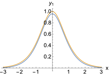
side in various scenarios near . First, let us look at the case when
both are single humped. We can always after rescaling take
. For simplicity we will also choose , and are then left with
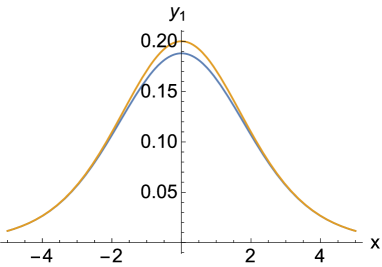
which for for illustrative purposes we will usually choose . For the choice
, , , ,
the left hand side of Eq. (II) is shown in blue and the right hand side in yellow
in Fig. 1.
Figure 1: lhs (blue- curve) vs. rhs of Eq. (II) for
when .
Here if we take the ratio we would find that this
was always less than over the entire range.
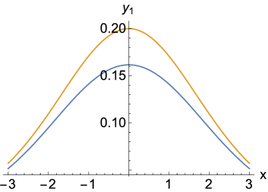
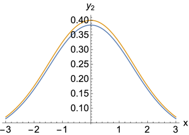
For this choice of parameters is much more modified by the interaction
than . This is shown in Figs. 2 and 3.
Figure 2: (upper curve) and when .Figure 3: (upper curve) and when .
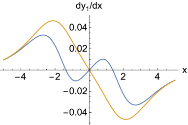
The problematic case is when one of the is double humped. In that case
the derivatives of determined from our approximation can be positive,
whereas the right hand side can still be negative in our approximation for a
range of small and . An example of this is given for the values:
, , , , in Fig. 4
Figure 4: lhs (blue) vs. rhs of Eq. (II) for when .
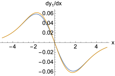
In this case if we reduce to be , then we again get good
agreement between the left and right hand sides of the equation for .
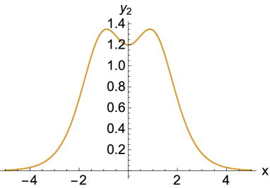
This is shown in Fig. 5. When , is
slightly modified from its value when . However, the double humped
solution is barely modified by the interaction as seen in
Figs. 6 and 7.
Figure 5: lhs vs. rhs of Eq. (II) for when .Figure 6: when (upper curve) vs. when .Figure 7: when vs. when (no visible difference at this scale.)
III Vector-Vector Interactions
The coupled nonlinear Dirac
equations (NLDEs) with vector-vector interactions are given by
(37)
(38)
Again by scaling , , we have only two
independent dimensionless coupling constants and
. Equations (37) and (38) can be derived from the
Lagrangian
(39)
We notice that as in the scalar-scalar case, the Lagrangian in this case is
also symmetric under the interchange ,
and . Again
using the representation as given by Eq. (10), we have the
equations for the components of the two coupled NLDEs which can be written as
(40)
These are symmetric under the interchange , and .
These four equations can also be written if we let as:
(41)
and
(42)
This reduces, when to the Eqs. (14) in Chang et al. Cha .
III.1 Conservation Laws
We again have energy-momentum conservation governed by Eqs.
(19) and (20) but where is now given by
Eq. (39).
From total momentum conservation, we find, just like for the scalar case,
that for a solution that vanishes at , and
are again given by Eqs. (21) and (22) respectively, but where
is as given by Eq. (39).
Multiplying Eq. (37) on the left by and Eq. (38)
on the left by and adding those two equations and then using
Eq. (22) to eliminate the interaction terms of ,
we as in the scalar case, again obtain Eq. (23). On using the ansatz
(10) we then again obtain
(43)
As in the scalar case, in the vector case too the energy and the charges
and are conserved and are again given by
Eqs. (26) to (28), respectively.
III.2 Approximate Solution
We will obtain our approximate analytic solution by assuming that each of
the two terms in Eq. (43) is identically zero. Then we obtain
(44)
whose solutions are given by Eq. (29).
We can again solve for and and obtain
So we see that we need both and for this
approximation to make sense. Now let us see to what extent we violate
Eq. III. We have, letting , the approximate
expression for , valid when , given by Eq. (29).
Now unlike the scalar-scalar case, the solutions are single humped and so typical values of the parameters give generic results.
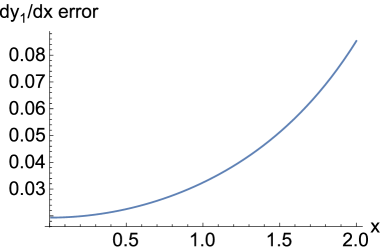
Setting and and , ,
, we find that the relative error on comparing
the lhs and rhs of Eq. (III), i.e , is less than
, (see Fig. 8 ) for , At the same time,
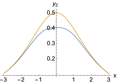
is changed quite a bit from its uncoupled value when we choose these values
of the parameters as seen in Fig. 9. The effect is not as dramatic
for for these values as seen in Fig. 10.
Figure 8: (lhs-rhs)/(lhs+rhs) of Eq. (III0 for when .Figure 9: (upper curve) and when .Figure 10: (upper curve) and when .
IV Nonrelativistic Limit
In our previous paper coo , we had started with NLD equations and using
Moore’s decoupling method moo we had obtained the nonrelativistic limit
of our NLD equations in both the scalar and the vector coupling cases.
In this section we essentially follow the same decoupling method to obtain
the nonrelativistic limit of coupled NLD equations in both scalar and
vector coupling cases.
Let us start from the coupled Eqs. (1) and (2) or
(37) and (38). They can be reexpressed in the form
(48)
(49)
where while
and is as given by Eq. (II) or (39).
On using
(50)
(51)
and the Moore’s decoupling method as well as essentially following the steps
given in our previous paper coo , we find that in both the
scalar-scalar and the vector-vector cases we get the coupled
NLS equations
(52)
(53)
under the assumption that and
.
Let us now look for exact solutions of the coupled Eqs. (52) and
(53) under the assumption that both and vanish in the
limit . It turns out that there are two such
solutions and we discuss these one by one.
IV.1 Solution I
It is easy to check that
(54)
is an exact solution to the coupled Eqs. (52) and (53) provided
provided . In case
then and remain undetermined and we
only have the constraint
(59)
IV.2 Solution II
Another solution to the coupled Eqs. (52) and (53) satisfying
the boundary condition
as is
(60)
provided
(61)
(62)
It is thus worth noting that while the first solution is valid for any values
of , the second solution is only valid when
.
V Conclusions
In this paper we have introduced and initiated discussion about coupled NLD
equations with both scalar-scalar and vector-vector interactions. In particular,
we have given the first (approximate) analytic solitary wave solution to two
coupled NLDEs for both scalar-scalar interactions and vector-vector interactions.
These solutions are relevant in nonlinear optics bar as well as for light solitons
in waveguide arrays lon ; dre ; tra among other applications in BECs and
cosmology. Further,we have shown using the Moore’s decoupling method that in
the nonrelativisticlimit, NLDEs with both scalar-scalar and vector-vector interactions
reduce tothe same coupled nonlinear Schrödinger equation (NLSE). We have
obtained two exact pulse solutions to these coupled NLSE.
Using the results found in coo , one can extend these solutions to the
case where the scalar-scalar as well as vector-vector interactions are taken
to an arbitrary (nonlinearity) power . We hope to address this issue
as well as the question of stability of the solutions found here in the near future.
Acknowledgements.
This work was performed in part under the auspices of the U.S.
Department of Energy. F.C. would like to thank the Santa Fe Institute and
the Center for Nonlinear Studies, Los Alamos National Laboratory, for its
hospitality. A.K. is grateful to Indian National Science Academy (INSA) for
awarding him INSA Senior Scientist position at Savitribai Phule Pune
University, Pune, India.