Experiments

Experimental Analysis of Algorithms for
Coflow Scheduling

Abstract

Modern data centers face new scheduling challenges in optimizing job-level performance objectives, where a significant challenge is the scheduling of highly parallel data flows with a common performance goal (e.g., the shuffle operations in MapReduce applications). Chowdhury and Stoica [6] introduced the coflow abstraction to capture these parallel communication patterns, and Chowdhury et al. [8] proposed effective heuristics to schedule coflows efficiently. In our previous paper [17], we considered the strongly NP-hard problem of minimizing the total weighted completion time of coflows with release dates, and developed the first polynomial-time scheduling algorithms with $O(1)$-approximation ratios.

In this paper, we carry out a comprehensive experimental analysis on a Facebook trace and extensive simulated instances to evaluate the practical performance of several algorithms for coflow scheduling, including our approximation algorithms developed in [17]. Our experiments suggest that simple algorithms provide effective approximations of the optimal, and that the performance of the approximation algorithm of [17] is relatively robust, near optimal, and always among the best compared with the other algorithms, in both the offline and online settings.

1 Introduction

Data-parallel computation frameworks such as MapReduce [9], Hadoop [1, 5, 18], Spark [20], Google Dataflow [2], etc., are gaining tremendous popularity as they become ever more efficient in storing and processing large-scale data sets in modern data centers. This efficiency is realized largely through massive parallelism. Typically, a datacenter job is broken down into smaller tasks, which are processed in parallel in a computation stage. After being processed, these tasks produce intermediate data, which may need to be processed further, and which are transferred between groups of servers across the datacenter network, in a communication stage. As a result, datacenter jobs often alternate between computation and communication stages, with parallelism enabling the fast completion of these large-scale jobs. While this massive parallelism contributes to efficient data processing, it presents many new challenges for network scheduling. In particular, traditional networking techniques focus on optimizing flow-level performance such as minimizing flow completion times, and ignore job-level performance metrics. However, since a computation stage often can only start after all parallel dataflows within a preceding communication stage have finished [7, 10], all these flows need to finish early to reduce the processing time of the communication stage, and of the entire job.

To faithfully capture application-level communication requirements, Chowdhury and Stoica [6] introduced the coflow abstraction, defined to be a collection of parallel flows with a common performance goal. Effective scheduling heuristics were proposed in [8] to optimize coflow completion times. In our previous paper [17], we developed scheduling algorithms with constant approximation ratios for the strongly NP-hard problem of minimizing the total weighted completion time of coflows with release dates, and conducted preliminary experiments to examine the practical performance of our approximation algorithms. These are the first $O(1)$-approximation algorithms for this problem. In this paper, we carry out a systematic experimental study on the practical performance of several coflow scheduling algorithms, including our approximation algorithms developed in [17]. Similar to [17], the performance metric that we focus on in this paper is the total weighted coflow completion time. As argued in [17], it is a reasonable user-oriented performance objective. It is also natural to consider other performance objectives, such as the total weighted flow time, which we leave as future work. Our experiments are conducted on real-world data gathered from Facebook and extensive simulated data, where we compare our approximation algorithm and its modifications to several other scheduling algorithms in an offline setting, and evaluate their relative performances, and compare them to an LP-based lower bound. The algorithms that we consider in this paper are characterized by several main components, such as the coflow order in which the algorithms follow, the grouping of the coflows, and the backfilling rules. We study the impact of each such component on the algorithm performance, and demonstrate the robust and near-optimal performance of our approximation algorithm [17] and its modifications in the offline setting, under the case of zero release times as well as general release times. We also consider online variants of the offline algorithms, and show that the online version of our approximation algorithm has near-optimal performance on real-world data and simulated instances.

The rest of this section is organized as follows. In Section 1.1, we quickly recall the problem formulation of coflow scheduling, the approximation algorithm of [17] as well as its approximation ratio. Section 1.2 gives an overview of the experimental setup and the main findings from our experiments. A brief review of related works is presented in Section 1.3.

1.1 Coflow Model and Approximation Algorithm

We consider a discrete-time system where $n$ coflows need to be scheduled in an $m\times m$ datacenter network with $m$ inputs and $m$ outputs. For each $k\in\{1,2,\cdots,n\}$, coflow $k$ is released at time $r_{k}$, and can be represented by an $m\times m$ matrix $D^{(k)}=\left(d_{ij}^{(k)}\right)_{i,j=1}^{m}$, where $d_{ij}^{(k)}$ is the number of data units (a.k.a. flow size) that need to be transferred from input $i$ to output $j$. The network has the so-called non-blocking switch architecture [3, 4, 12, 16], so that a data unit that is transferred out of an input is immediately available at the corresponding output. We also assume that all inputs and outputs have unit capacity. Thus, in a time slot, each input/output can process at most one data unit; similar to [17], these restrictions are called matching constraints. Let $C_{k}$ denote the completion time of coflow $k$, which is the time when all data units from coflow $k$ have finished being transferred. We are interested in developing efficient (offline) scheduling algorithms that minimize $\sum_{k=1}^{n}w_{k}C_{k}$, the total weighted completion time of coflows, where $w_{k}$ is a weight parameter associated with coflow $k$.

A main result of [17] is the following theorem.

Theorem 1

[17] There exists a deterministic polynomial time $67/3$-approximation algorithm for the coflow scheduling problem, with the objective of minimizing the total weighted completion time.

The approximation algorithm of [17] consists of two related stages. First, a coflow order is computed by solving a polynomial-sized interval-indexed linear program (LP) relaxation, similar to many other scheduling algorithms (see e.g., [11]). Then, we use this order to derive an actual schedule. To do so, we define a grouping rule, under which we partition coflows into a polynomial number of groups, based on the minimum required completion times of the ordered coflows, and schedule the coflows in the same group as a single coflow optimally, according to an integer version of the Birkhoff-von Neumann decomposition theorem. The description of the algorithm is given in Algorithm 4 of the Appendix for completeness. Also see [17] for more details. From now on, the approximation algorithm of [17] will be referred to as the LP-based algorithm.

1.2 Overview of Experiments

Since our LP-based algorithm consists of an ordering and a scheduling stage, we are interested in algorithmic variations for each stage and the performance impact of these variations. More specifically, we examine the impact of different ordering rules, coflow grouping and backfilling rules, in both the offline and online settings. Compared with the very preliminary experiments we did in [17], in this paper we conduct a substantially more comprehensive study by considering many more ordering and backfilling rules, and examining the performance of algorithms on general instances in addition to real-world data. We also consider the offline setting with general release times, and online extensions of algorithms, which are not discussed in [17].

Workload.

Our evaluation uses real-world data, which is a Hive/MapReduce trace collected from a large production cluster at Facebook [7, 8, 17], as well as extensive simulated instances.

For real-world data, we use the same workload as described in [8, 17]. The workload is based on a Hive/MapReduce trace at Facebook that was collected on a 3000-machine cluster with 150 racks, so the datacenter in the experiments can be modeled as a $150\times 150$ network switch (and coflows be represented by $150\times 150$ matrices). We select the time unit to be 1/128 second (see [17] for details) so that each port has the capacity of 1MB per time unit. We filter the coflows based on the number of non-zero flows, which we denote by $M^{\prime}$, and we consider three collections of coflows, filtered by the conditions $M^{\prime}\geq 25$, $M^{\prime}\geq 50$ and $M^{\prime}\geq 100$, respectively.

We also consider synthetic instances in addition to the real-world data. For problem size with $k$ = 160 coflows and $m$ = 16 inputs and outputs, we randomly generate 30 instances with different numbers of non-zero flows involved in each coflow. For instances 1-5, each coflow consists of $m$ flows, which represent sparse coflows. For instances 5-10, each coflow consists of $m^{2}$ flows, which represent dense coflows. For instances 11-30, each coflow consists of $u$ flows, where u is uniformly distributed on $\{m,\cdots,m^{2}\}$. Given the number $k$ of flows in each coflow, $k$ pairs of input and output ports are chosen randomly. For each pair of $(i,j)$ that is selected, an integer processing requirement $d_{i,j}$ is randomly selected from the uniform distribution on $\{1,2,\cdots,100\}$.

Our main experimental findings are as follows:

• Algorithms with coflow grouping consistently outperform those without grouping. Similarly, algorithms that use backfilling consistently outperform those that do not use backfilling. The benefit of backfilling can be further improved by using a balanced backfilling rule (see §3.2 for details).

• The performance of the LP-based algorithm and its extensions is relatively robust, and among the best compared with those that use other simpler ordering rules, in the offline setting.

• In the offline setting with general release times, the magnitude of inter-arrival times relative to the processing times can have complicated effects on the performance of various algorithms. (see §4.1 for details).

• The LP-based algorithm can be extended to an online algorithm and has near-optimal performance.

1.3 Related Work

There has been a great deal of success over the past 20 years on combinatorial scheduling to minimize average completion time, see e.g., [11, 14, 15, 19], typically using a linear programming relaxation to obtain an ordering of jobs and then using that ordering in some other polynomial-time algorithm. There has also been success in shop scheduling. We do not survey that work here, but note that traditional shop scheduling is not “concurrent”. In the language of our problem, that would mean that two flows in the same coflow could not be processed simultaneously. The recently studied concurrent open shop problem removes this restriction and models flows that can be processed in parallel. There is a close connection between concurrent open shop problem and coflow scheduling problem. When all coflow matrices are diagonal, coflow scheduling is equivalent to a concurrent open shop scheduling problem [8, 17]. Leung et al. [13] presented heuristics for the total completion time objective and conducted an empirical analysis to compare the performance of different heuristics for concurrent open shop problem. In this paper, we consider a number of heuristics that include natural extensions of heuristics in [13] to coflow scheduling.

2 Preliminary Background

In [17], we formulated the following interval-indexed linear program (LP) relaxation of the coflow scheduling problem, where $\tau_{l}$’s are the end points of a set of geometrically increasing intervals, with $\tau_{0}=0$, and $\tau_{l}=2^{l-1}$ for $l\in\{1,2,\ldots,L\}$. Here $L$ is such that $\tau_{L}=2^{L-1}$ is an upper bound on the time that all coflows are finished processing under any optimal algorithm.

$$(LP)\hskip 14.22636pt\mbox{Minimize }\sum_{k=1}^{n}w_{k}\sum_{l=1}^{L}\tau_{l-1}x_{l}^{(k)}\quad\quad\mbox{ subject to }$$

$$\sum_{u=1}^{l}\sum_{k=1}^{n}\sum_{j^{\prime}=1}^{m}d_{ij^{\prime}}^{(k)}x_{u}^{(k)}\leq\tau_{l},\mbox{ for }i=1,\ldots,m,\;l=1,\ldots,L;$$ (1)

$$\sum_{u=1}^{l}\sum_{k=1}^{n}\sum_{i^{\prime}=1}^{m}d_{i^{\prime}j}^{(k)}x_{u}^{(k)}\leq\tau_{l},\mbox{ for }j=1,\ldots,m,\;l=1,\ldots,L;$$ (2)

$$x_{l}^{(k)}=0\mbox{ if }{r_{k}+}\sum_{j^{\prime}=1}^{m}d_{ij^{\prime}}^{(k)}>\tau_{l}\mbox{ or }{r_{k}+}\sum_{i^{\prime}=1}^{m}d_{i^{\prime}j}^{(k)}>\tau_{l};$$ (3)

$$\sum_{l=1}^{L}x_{l}^{(k)}=1,\mbox{ for }k=1,\ldots,n;$$

$$x_{l}^{(k)}\geq 0,\mbox{ for }k=1,\ldots,n,\ l=1,\ldots,L.$$

For each $k$ and $l$, $x_{l}^{(k)}$ can be interpreted as the LP-relaxation of the binary decision variable which indicates whether coflow $k$ is scheduled to complete within the interval $(\tau_{l-1},\tau_{l}]$. Constraints (1) and (2) are the load constraints on the inputs and outputs, respectively, which state that the total amount of work completed on each input/output by time $\tau_{l}$ cannot exceed $\tau_{l}$, due to matching constraints. Constraint (3) takes into account of the release times.

(LP) provides a lower bound on the optimal total weighted completion time of the coflow scheduling problem. If, instead of being end points of geometrically increasing time intervals, $\tau_{l}$ are end points of the discrete time units, then (LP) becomes exponentially sized (which we refer to as (LP-EXP)), and gives a tighter lower bound, at the cost of longer running time. (LP) computes an approximated completion time $\bar{C}_{k}=\sum_{l=1}^{L}\tau_{l-1}\bar{x}_{l}^{(k)}$, for each $k$, based on which we re-order and index the coflows in a nondecreasing order of $\bar{C_{k}}$, i.e.,

$$\bar{C}_{1}\leq\bar{C}_{2}\leq\ldots\leq\bar{C}_{n}.$$ (4)

3 Offline Algorithms with Zero Release Time

In this section, we assume that all the coflows are released at time 0. We compare our LP-based algorithm with others that are based on different ordering, grouping, and backfilling rules.

3.1 Ordering Heuristics

An intelligent ordering of coflows in the ordering stage can substantially reduce coflow completion times. We consider the following five greedy ordering rules, in addition to the LP-based order (4), and study how they affect algorithm performance.

Definition 1

The First in first (FIFO) heuristic orders the coflows arbitrarily (since all coflows are released at time $0$).

Definition 2

The Shortest Total Processing Time first (STPT) heuristic orders the coflows based on the total amount of processing requirements over all the ports, i.e., $\sum_{i=1}^{m}\sum_{j=1}^{m}{d_{ij}}$.

Definition 3

The Shortest Maximum Processing Time first (SMPT) heuristic orders the coflows based on the load $\rho$ of the coflows, where $\rho=\max\{\displaystyle\max_{i=1,\ldots,m}\eta_{i}$,
$\displaystyle\max_{j=1,\ldots,m}\theta_{j}\}$, $\eta_{i}=\{\sum_{j^{\prime}=1}^{m}{d_{ij^{\prime}}}\}$ is the load on input $i$, and $\theta_{j}=\{\sum_{i^{\prime}=1}^{m}{d_{i^{\prime}j}}\}$ is the load on output $j$.

Definition 4

To compute a coflow order, the Smallest Maximum Completion Time first (SMCT) heuristic treats all inputs and outputs as $2m$ independent machines. For each input $i$, it solves a single-machine scheduling problem where $n$ jobs are released at time $0$, with processing times $\eta_{i}^{(k)}$, $k=1,2,\cdots,n$, where $\eta_{i}^{(k)}$ is the $i$th input load of coflow $k$. The jobs are sequenced in the order of increasing $\eta_{i}^{(k)}$, and the completion times $C^{(i)}(k)$ are computed. A similar problem is solved for each output $j$, where jobs have processing times $\theta_{j}^{(k)}$, and the completion times $C_{(j)}(k)$ are computed. Finally, the SMCT heuristic computes a coflow order according to non-decreasing values of $C^{\prime}(k)=\displaystyle\max_{i,j}\{C^{(i)}(k),C_{(j)}(k)\}$.

Definition 5

The Earliest Completion Time first (ECT) heuristic generates a sequence of coflow one at a time; each time it selects as the next coflow the one that would be completed the earliest.

3.2 Scheduling via Birkhoff-von Neumann Decomposition, Backfilling and Grouping

The derivation of the actual sequence of schedules in the scheduling stage of our LP-based algorithm relies on two key ideas: scheduling according to an optimal (Birkhoff-von Neumann) decomposition, and a suitable grouping of the coflows. It is reasonable to expect grouping to improve algorithm performance, because it may consolidate skewed coflow matrices to form more balanced ones that can be scheduled more efficiently. Thus, we compare algorithms with grouping and those without grouping to understand its effect. The particular grouping procedure that we consider here is the same as that in [17] (also see Step 2 of Algorithm 4 of the Appendix), and basically groups coflows into geometrically increasing groups, based on aggregate demand. Coflows of the same group are treated as a single, aggregated coflow, and this consolidated coflow is scheduled according to the Birkhoff-von Neumann decomposition (see [17] or Algorithm 5 of the Appendix).

Backfilling is a common strategy used in scheduling for computer systems to increase resource utilization (see, e.g. [8]). While it is difficult to analytically characterize the performance gain from backfilling in general, we evaluate its performance impact experimentally. We consider two backfilling rules, described as follows. Suppose that we are currently scheduling coflow $D$. The schedules are computed using the Birkhoff-von Neumann decomposition, which in turn makes use of a related, augmented matrix $\tilde{D}$, that is component-wise no smaller than $D$. The decomposition may introduce unforced idle time, whenever $D\neq\tilde{D}$. When we use a schedule that matches input $i$ to output $j$ to serve the coflow with $D_{ij}<\tilde{D}_{ij}$, and if there is no more service requirement on the pair of input $i$ and output $j$ for the coflow, we backfill in order from the flows on the same pair of ports in the subsequent coflows. When grouping is used, backfilling is applied to the aggregated coflows. The two backfilling rules that we consider – which we call backfilling and balanced backfilling – are only distinguished by the augmentation procedures used, which are, respectively, the augmentation used in [17] (Step 1 of Algorithm 5) and the balanced augmentation described in Algorithm 1.

The balanced augmentation (Algorithm 1) results in less skewed matrices than the augmentation step in [17], since it first “spreads out” the unevenness among the components of a coflow. To illustrate, let

$$D=\left(\begin{array}[]{ccc}10&0&0\\ 10&0&0\\ 10&0&0\\ \end{array}\right),B=\left(\begin{array}[]{ccc}10&10&10\\ 10&10&10\\ 10&10&10\\ \end{array}\right),\mbox{ and }C=\left(\begin{array}[]{ccc}10&20&0\\ 10&0&20\\ 10&10&10\\ \end{array}\right).$$

Under the balanced augmentation, $D$ is augmented to $B$ and under the augmentation of [17], $D$ is augmented to $C$.

Data: A single coflow $D=\left({d}_{ij}\right)_{i,j=1}^{m}$.

Result: A matrix $\tilde{D}=\left({\tilde{d}}_{ij}\right)_{i,j=1}^{m}$ with equal row and column sums, and $D\leq\tilde{D}$.

Let $\rho$ be the load of $D$.

$p_{i}\leftarrow\rho-\sum_{j^{\prime}=1}^{m}d_{ij^{\prime}}$, for $i=1,2,\ldots,m.$

$q_{i}\leftarrow\rho-\sum_{i^{\prime}=1}^{m}d_{i^{\prime}j}$, for $j=1,2,\ldots,m.$

$\Delta\leftarrow m\rho-\sum_{i=1}^{m}\sum_{j=1}^{m}d_{ij}.$

$d^{\prime}_{ij}=\lfloor d_{ij}+p_{i}q_{i}/\Delta\rfloor.$

Augment $D^{\prime}=(d^{\prime}_{ij})$ to a matrix $\tilde{D}$ with equal row and column sums (see Step 1 of Algorithm 5 of the Appendix; also see [17]).

Algorithm 1 Balanced Coflow Augmentation

3.3 Scheduling Algorithms and Metrics

We consider $30$ different scheduling algorithms, which are specified by the ordering used in the ordering stage, and the actual sequence of schedules used in the scheduling stage. We consider 6 different orderings described in §3.1, and the following $5$ cases in the scheduling stage:

• (a) without grouping or backfilling, which we refer to as the base case;

• (b) without grouping but with backfilling;

• (c) without grouping but with balanced backfilling;

• (d) with grouping and with backfilling;

• (e) with grouping and with balanced backfilling.

We will refer to these cases often in the rest of the paper. Our LP-based algorithm (Algorithm 4 in the Appendix) corresponds to the combination of LP-based ordering and case (d).

For ordering, six different possibilities are considered. We use $H_{A}$ to denote the ordering of coflows by heuristic $A$, where $A$ is in the set $\{$FIFO, STPT, SMPT, SMCT, ECT$\}$, and $H_{LP}$ to denote the LP-based coflow ordering. Note that in [17], we only considered orderings $H_{FIFO},H_{SMPT}$ and $H_{LP}$, and cases (a), (b) and (d) for scheduling, and their performance on the Facebook trace.

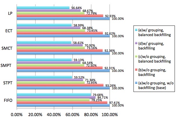
(a) Comparison of total weighted completion times normalized using the base case (e) for each order

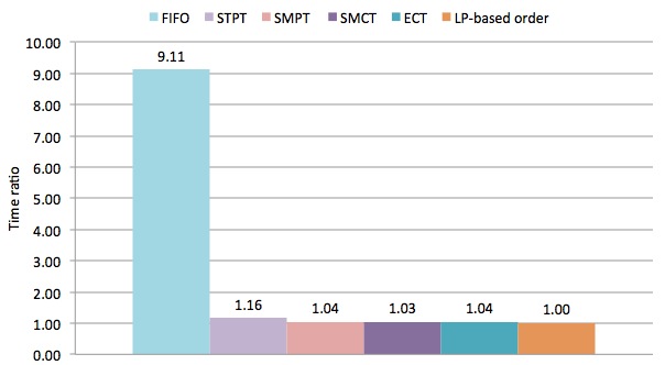
(b) Comparison of 6 orderings with zero release times on Facebook data.

Figure 1: Facebook data are filtered by $M^{\prime}\geq 50$. Weights are equal.

3.4 Performance of Algorithms on Real-World Data

We compute the total weighted completion times for all 6 orders in the 5 different cases (a) – (e) described in §3.3, through a set of experiments on filtered coflow data. We present representative comparisons of the algorithms here.

Figure 1a plots the total weighted completion times as percentages of the base case (a), for the case of equal weights. Grouping and backfilling both improve the total weighted completion time with respect to the base case for all 6 orders. In addition to the reduction in the total weighted completion time from backfilling, which is up to 7.69%, the further reduction from grouping is up to 24.27%, while the improvement from adopting the balanced backfilling rule is up to 20.31%. For 5 non-arbitrary orders (excluding FIFO), scheduling with both grouping and balanced backfilling (i.e., case (e)) gives the smallest total weighted completion time.

We then compare the performances of different coflow orderings. Figure 1b shows the comparison of total weighted completion times evaluated on filtered coflow data in case (e) where the scheduling stage uses both grouping and balanced backfilling. Compared with $H_{FIFO}$, all other ordering heuristics reduce the total weighted completion times of coflows by a ratio between 7.88 and 9.11, with $H_{LP}$ performing consistently better than other heuristics.

3.5 Cost of Matching

The main difference between our coflow scheduling problem and the well-studied concurrent open shop problem we discussed in §1.3 is the presence of matching constraints on paired resources, i.e. inputs and outputs, which is the most challenging part in the design of approximation algorithms [17]. Since our approximation algorithm handles matching constraints, it is more complicated than scheduling algorithms for concurrent open shop problem. We are interested in how much we lose by imposing these matching constraints.

To do so, we generate two sets of coflow data from the Facebook trace. For each coflow $k$, let the coflow matrix $D^{(k)}$ be a diagonal matrix, which indicates that coflow $k$ only has processing requirement from input $i$ to output $i$, for $i=1,\ldots,m$. The processing requirement $D_{i,i}^{(k)}$ is set to be equal to the sum of all dataflows of coflow $k$ in the Facebook trace that require processing from input $i$. We then construct coflow matrix $\tilde{D}^{(k)}$ such that $\tilde{D}^{(k)}$ is not diagonal and has the same row sum and column sum as $D^{(k)}$. The details of the generation is described as in Algorithm 2.

The diagonal structured coflow matrices can reduce the total completion time of by a ratio up to 2.09, which indicates the extra processing time introduced by the matching constraints.

3.6 Performance of Algorithms on General Instances

In previous sections, we present the experimental results of several algorithms on the Facebook trace. In order to examine the consistency of the performance of these algorithms, we consider more instances, including examples where certain algorithms behave badly.

3.6.1 Bad Instances for Greedy Heuristics

We consider the following examples which illustrate instances on which the ordering heuristics do not perform well.

Example 1

Consider a $2\times 2$ network and $n$ coflows with $D=\left(\begin{array}[]{cc}10&0\\ 0&0\end{array}\right)$, $n$ coflows with $D=\left(\begin{array}[]{cc}0&0\\ 0&10\end{array}\right)$, and $a\cdot n$ coflows with $D=\left(\begin{array}[]{cc}9&0\\ 0&9\end{array}\right)$. The optimal schedule in this case is to schedule the orders with the smallest total processing time first, i.e., the schedule is generated according to the STPT rule. The limit of the ratio $\frac{\sum_{k=1}^{n}C_{k}(ECT\&SMCT\&SMPT)}{\sum_{k=1}^{n}C_{k}(STPT)}$ is increasing in $n$ and when $n\rightarrow\infty$ it becomes $\frac{a^{2}+4a+2}{a^{2}+2a+2}$. This ratio reaches its maximum of $\sqrt{2}$ when $a=\sqrt{2}$.

We can generalize this counterexample to an arbitrary number of inputs and outputs $m$. To be more specific, in an $m\times m$ network, for $j=1,2,\cdots,m$, we have $n$ coflows only including flows to be transferred to output $j$, i.e., $d_{ij}=10$. We also have $a\cdot n$ coflows with equal transfer requirement on all pairs of inputs and outputs, i.e., $d_{ij}=9$ for $i,j=1,2,\cdots,m$. The ratio

$$\lim_{n\rightarrow\infty}\frac{\sum_{k=1}^{n}C_{k}(ECT\&SMCT\&SMPT)}{\sum_{k=1}^{n}C_{k}(STPT)}=\frac{a^{2}+2ma+m}{a^{2}+2a+m}$$

has a maximum value of $\sqrt{m}$ when $a=\sqrt{m}$. Note that in the generalized example, we need to consider the matching constraints when we actually schedule the coflows.

Example 2

Consider a $2\times 2$ network and $n$ coflows with $D=\left(\begin{array}[]{cc}1&0\\ 0&10\end{array}\right)$, and $a\cdot n$ coflows with $D=\left(\begin{array}[]{cc}10&0\\ 0&0\end{array}\right)$. The optimal schedule in this case is to schedule the orders with the Smallest Maximum Completion Time first, i.e., the schedule is generated according to the SMCT rule. The ratio $\frac{\sum_{k=1}^{n}C_{k}(STPT)}{\sum_{k=1}^{n}C_{k}(SMCT)}$ is increasing in $n$ and when $n\rightarrow\infty$ it becomes $\frac{a^{2}+2a}{a^{2}+1}$ This ratio reaches its maximum of $\frac{\sqrt{5}+1}{2}$ when $a=\frac{\sqrt{5}+1}{2}$.

This counterexample can be generalized to an arbitrary number of inputs and outputs $m$. In an $m\times m$ network, for each $i=2,3,\cdots,m$, we have $n$ coflows with two nonzero entries, $d_{11}=1$ and $d_{ii}=10$. We also have $a\cdot n$ coflows with only one zero entry $d_{11}=10$. The limit of the ratio

$$\lim_{n\rightarrow\infty}\frac{\sum_{k=1}^{n}C_{k}(STPT)}{\sum_{k=1}^{n}C_{k}(SMCT)}=\frac{a^{2}+2(m-1)a}{a^{2}+m-1}$$

has a maximum value of $1/2+\sqrt{m-3/4}$ when $a=1/2+\sqrt{m-3/4}$.

3.6.2 General instances

We present comparison of total weighted completion time for 6 orderings and 5 cases on general simulated instances as described in §1.2, in Appendix Tables 1 to 5, normalized with respect to the LP-based ordering in case (c), which performs best on all of the instances. We have the similar observation from the general instances that both grouping and backfilling reduce the completion time. However, under balanced backfilling, grouping does not improve performance much. Both grouping and balanced backfilling form less skewed matrices that can be scheduled more efficiently, so when balanced backfilling is used, the effect of grouping is less pronounced. It is not clear whether case (c) with balanced backfilling only is in general better than case (e) with both balanced backfilling and grouping, as we have seen Facebook data on which case (e) gives the best result. As for the performance of the orderings, on the one hand, we see in Table 3 very close time ratios among all the non-arbitrary orderings on instances 6 - 30, and a better performance of $H_{ECT}$ on sparse instances 1 - 5 over other orderings; on the other hand, there are also instances where ECT performs poorly (see §3.6.1 for details).

Besides their performance, the running times of the algorithms that we consider are also important. The running time of an algorithm consists of two main parts; computing the ordering and computing the schedule. On a Macbook Pro with 2.53 GHz two processor cores and 6G memory, the five ordering rules, FIFO, STPT, SMPT, SMCT and ECT, take less than 1 second to compute, whereas the LP-based order can take up to 90 seconds. Scheduling with backfilling can be computed in around 1 minute, whereas balanced backfilling computes the schedules with twice the amount of time, beause the balanced augmented matrices have more non-zero entries. Besides improving performance, grouping can also reduce the running time by up to 90%.

Data: A single diagonal coflow $D=\left({d}_{ij}\right)_{i,j=1}^{m}$.

Result: Another coflow $\tilde{D}=\left({\tilde{d}}_{ij}\right)_{i,j=1}^{m}$, such that row and column sums of the two matrices are all equal.

Let $\eta(\tilde{D})=\sum_{i,j=1}^{m}{\tilde{d}_{ij}}$ be the sum of all entries in $\tilde{D}$. Similarly, $\eta(D)=\sum_{i=1}^{m}d_{ii}$.

$\tilde{D}\leftarrow 0$.

while $(\eta(\tilde{D})<\eta(D))$ do

      $S_{i}\leftarrow\{i:\sum_{j^{\prime}=1}^{m}{\tilde{D}_{ij^{\prime}}}<d_{ii}\}$; $S_{j}\leftarrow\{j:\sum_{i^{\prime}=1}^{m}{\tilde{D}_{i^{\prime}j}}<d_{jj}\}$. Randomly pick $i^{*}$ from set $S_{i}$ and $j^{*}$ from set $S_{j}$. $\tilde{D}\leftarrow\tilde{D}+pE,$ where $p=\min\{d_{i^{*}i^{*}}-\sum_{j^{\prime}=1}^{m}{\tilde{D}_{i^{*}j^{\prime}}},d_{j^{*}j^{*}}-\sum_{i^{\prime}=1}^{m}{\tilde{D}_{i^{\prime}j^{*}}}\}$, $E_{ij}=1$ if $i=i^{*}$ and $j=j^{*}$, and $E_{ij}=0$ otherwise.

      $\eta\leftarrow\sum_{i,j=1}^{m}{\tilde{d}_{ij}}$

      end while

Algorithm 2 Construction of coflow data

4 Offline Algorithms with General Release Times

In this section, we examine the performances of the same class of algorithms and heuristics as that studied in Section 3, when release times can be general. We first extend descriptions of various heuristics to account for release times.

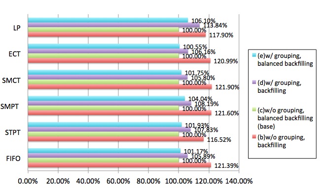
(a) Comparison of total weighted completion times normalized using the base case (c) for each order.

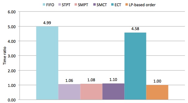
(b) Comparison of 6 orderings with general release times on Facebook data.

Figure 2: Facebook data are filtered by $M^{\prime}\geq 50$. Weights are equal.

The FIFO heuristic computes a coflow order according to non-decreasing release time $r$. (Note that when all release times are distinct, FIFO specifies a unique ordering on coflows, instead of any arbitrary order in the case of zero release times.) The STPT heuristic computes a coflow order according to non-decreasing values of $\sum_{i=1}^{m}\sum_{j=1}^{m}{d_{ij}}+r$, the total amount of processing requirements over all the ports plus the release time. The SMPT heuristic computes a coflow order according to non-decreasing values of $\rho+r$, the sum of the coflow load and release time. Similar to the case of zero release times, the SMCT heuristic first sequences the coflows in non-decreasing order of $\sum_{j^{\prime}}d_{ij^{\prime}}+r$ on each input $i$ and $\sum_{i^{\prime}}d_{i^{\prime}j}+r$ on each output $j$, respectively, and then computes the completion times $C^{(i)}$ and $C_{(j)}$, treating each input and output as independent machines. Finally, the coflow order is computed according to non-decreasing values of $C^{\prime}=\max_{i,j}\{C^{(i)},C_{(j)}\}$. The ECT heuristic generates a sequence of coflows one at a time; each time it selects as the next coflow the one that has been released and is after the preceding coflow finishes processing and would be completed the earliest.

We compute the total weighted completion time for 6 orderings (namely, the LP-based ordering (4) and the orderings from definitions with release times and cases (b) - (e) (recall the description of these cases at the beginning of Section 3.3), normalized with respect to the LP-based ordering in case (c). The results for Facebook data are illustrated in Figure 2a and Figure 2b. For general instances, we generate the coflow inter-arrival times from uniform distribution [1, 100] and present the ratios in Tables 6 to 9 in the Appendix. As we can see from e.g., Figure 2a, the effects of backfilling and grouping on algorithm performance are similar to those noted in §3.6.2, where release times are all zero. The STPT and LP-based orderings STPT appear to perform the best among all the ordering rules (see Figure 2b), because the magnitudes of release times have a greater effect on FIFO, SMPT, SMCT and ECT than they do on STPT.

By comparing Figures 1b and 2b, we see that ECT performs much worse than it does with common release times. This occurs because with general release times, ECT only schedules a coflow after a preceding coflow completes, so it does not backfill. While we have kept the ECT ordering heuristic simple and reasonable to compute, no backfilling implies larger completion times, hence the worse performance.

4.1 Convergence of Heuristics with Respect to Release Times

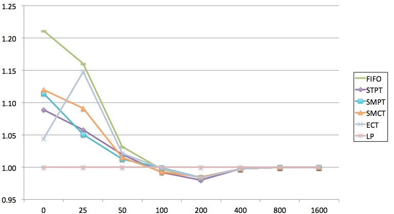
(a) Number of flows is $16$

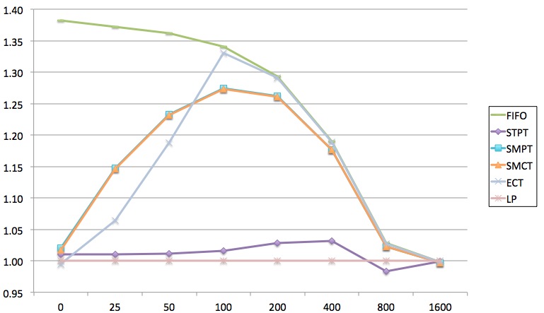
(b) Number of flows is uniform in $[16,256]$

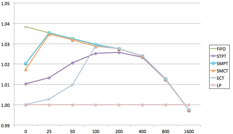
(c) Number of flows is $256$

Figure 3: Comparison of total weighted completion times with respect to the upper bound of inter-arrival time for each order on general instances. Network size is $16$. Number of Coflow is 160.

In order to have a better understanding of release times, we scale the release times of the coflows and observe the impact of release time distribution on the performance of different heuristics. For general instances, recall that we generated the inter-arrival times with an upper bound of 100. Here we also consider inter-arrival time distributions that are uniform over [0, 0], [0, 25], [0, 50], [0, 200], [0, 400], [0, 800] and [0, 1600], respectively. We compute the total weighted completion time with the adjusted release times in each case for 250 samples and take the average ratio with respect to the LP-based order.

As we can see from Figures 3a to 3c, all the heuristics converge to FIFO as the inter-arrival time increases. This is reasonable as the release times dominate the ordering when they are large. The speed of convergence is higher in 3a where the coflow matrices in the instance are sparse and release times are more influential in all heuristics. On the contrary, when the coflow matrices are dense, release times weigh less in heuristics, which converge slower to FIFO as shown in 3c. We also note that for heuristics other than FIFO, the relative performance of an ordering heurstic with respect to the LP-based order may deteriorate and then improve, as we increase the inter-arrival times. This indicates that when inter-arrival times are comparable to the coflow sizes, they can have a significant impact on algorithm performance and the order obtained.

5 Online Algorithms

We have discussed the experimental results of our LP-based algorithm and several heuristics in the offline setting, where the complete information of coflows is revealed at time $0$. In reality, information on coflows (i.e., flow sizes) is often only revealed at their release times, i.e., in an online fashion. It is then natural to consider online modifications of the offline algorithms considered in earlier sections. We proceed as follows. For the ordering stage, upon each coflow arrival, we re-order the coflows according to their remaining processing requirements. We consider all six ordering rules described in §3. For example, the LP-based order is modified upon each coflow arrival, by re-solving the (LP) using the remaining coflow sizes (and the newly arrived coflow) at the time. We describe the online algorithm with LP-based ordering in Algorithm 3. For the scheduling stage, we use case (c) the balanced backfilling rule without grouping, because of its good performance in the offline setting.

Data: Coflows $\left(d^{(k)}_{ij}\right)_{i,j=1}^{m}$ with different release times, for $k=1,\ldots,n$.

Result: A scheduling algorithm that uses at most a polynomial number of different matchings.

• Step 1: Given $n_{a}$ coflows in the system, $n_{a}\leq n$, solve the linear program (LP). Let an optimal solution be given by $\bar{x}_{l}^{(k)}$, for $l=1,2,\ldots,L$ and $k=1,2,\ldots,n_{a}$. Compute the approximated completion time $\bar{C}_{k}$ by

  $$\bar{C}_{k}=\sum_{l=1}^{L}\tau_{l-1}\bar{x}_{l}^{(k)}.$$

  Order and index the coflows according to

  $$\bar{C}_{1}\leq\bar{C}_{2}\leq\ldots\leq\bar{C}_{n_{a}}.$$

• Step 2: Schedule the coflows in order using Algorithm 5 until an release of a new coflow. Update the job requirement with the remaining job for each coflow in the system and go back to Step 1.

Algorithm 3 Online LP-based Approximation

We compare the performance of the online algorithms and we compare the online algorithms to the offline algorithms. We improve the time ratio for all the orderings except FIFO by allowing re-ordering and preemption in the online algorithm compared with the static offline version. Note that we do not preempt with FIFO order. While several ordering heuristics perform as well as LP-based ordering in the online algorithms, a natural question to ask is how close $H_{A}$’s are to the optimal, where $A\in\{STPT,SMPT,SMCT,ECT,LP\}$. In order to get a tight lower bound of the coflow scheduling problem, we solve (LP-EXP) for sparse instances. Since it is extremely time consuming to solve (LP-EXP) for dense instances, we consider a looser lower bound, which is computed as follows. We first aggregate the job requirement on each input and output and solve a single machine scheduling problem for the total weighted completion time, on each input/output. The lower bound is obtained by taking the maximum of the results. The lower bounds are shown in the last column of Table 11. The ratio of the lower bound over the weighted completion time under $H_{LP}$ is in the range of $0.91$ to $0.97$, which indicates that it provides a good approximation of the optimal.

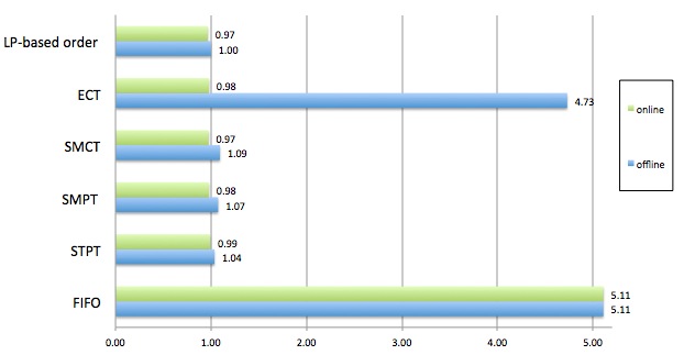
Figure 4: Comparison of total weighted completion times with respect to the base case for each order under the offline and online algorithms. Data are filtered by $M^{\prime}\geq 50$. Weights are equal.

6 Conclusion

We have performed comprehensive experiments to evaluate different scheduling algorithms for the problem of minimizing the total weighted completion time of coflows in a datacenter network. We also generalize our algorithms to an online version for them to work in real-time. For additional interesting directions in experimental analysis of coflow scheduling algorithms, we would like to come up with structured approximation algorithms that take into consideration other metrics and the addition of other realistic constraints, such as precedence constraints, and distributed algorithms that are more suitable for implementation in a data center. These new algorithms can be used to design other implementable, practical algorithms.

Acknowledgment

Yuan Zhong would like to thank Mosharaf Chowdhury and Ion Stoica for numerous discussions on the coflow scheduling problem, and for sharing the Facebook data.

APPENDIX

Appendix 0.A Algorithms

0.A.1 Offline Algorithm

We describe our offline LP-based approximation algorithm [17] in detail in Algorithm 4:

Data: Coflows $\left(d^{(k)}_{ij}\right)_{i,j=1}^{m}$, for $k=1,\ldots,n$.

Result: A scheduling algorithm that uses at most a polynomial number of different matchings.

• Step 1 (ordering): Given $n$ coflows, solve the linear program (LP). Let an optimal solution be given by $\bar{x}_{l}^{(k)}$, for $l=1,2,\ldots,L$ and $k=1,2,\ldots,n$. Compute the approximated completion time $\bar{C}_{k}$ by

  $$\bar{C}_{k}=\sum_{l=1}^{L}\tau_{l-1}\bar{x}_{l}^{(k)}.$$

  Order and index the coflows according to

  $$\bar{C}_{1}\leq\bar{C}_{2}\leq\ldots\leq\bar{C}_{n}.$$

• Step 2 (scheduling): For each $k$, $k=1,2,\ldots n,$ compute the maximum total input load $I_{k}$, the maximum total output load $J_{k}$ and the maximum total load $V_{k}$ by

  $$\hfill I_{k}=\max_{i=1,\ldots,m}\Bigg{\{}\sum_{j^{\prime}=1}^{m}\sum_{g=1}^{k}{d_{ij^{\prime}}^{(g)}}\Bigg{\}}\mbox{ , }J_{k}=\max_{j=1,\ldots,m}\Bigg{\{}\sum_{i^{\prime}=1}^{m}\sum_{g=1}^{k}{d_{i^{\prime}j}^{(g)}}\Bigg{\}}\hfill$$

  $$\hfill\mbox{ and }\quad V_{k}=\max\{I_{k},J_{k}\}.\hfill$$

  Suppose that $V_{k}\in(\tau_{r(k)-1},\tau_{r(k)}]$ for some function $r(\cdot)$ of $k$. Let the range of function $r(\cdot)$ consist of values $s_{1}<s_{2}<\ldots<s_{P}$, and define the sets $S_{u}=\left\{k:\tau_{s_{u}-1}<V_{k}\leq\tau_{s_{u}}\right\}$, $u=1,2,\ldots,P$.

$u\leftarrow 1$.

while $u\leq P$ do

       After all the coflows in set $S_{u}$ are released, schedule them as a single coflow with transfer requirement $\sum_{k\in S_{u}}d_{ij}^{(k)}$ from input $i$ to output $j$ and finish processing the coflow using Algorithm 5.

       $u\leftarrow u+1$;

      

end while

Algorithm 4 Offline LP-based Approximation

The Birkhoff-von Neumann decomposition that produces an optimal schedule for a coflow is described in detail in Algorithm 5.

Data: A single coflow $D=\left({d}_{ij}\right)_{i,j=1}^{m}$.

Result: A scheduling algorithm that uses at most a polynomial number of different matchings.

• Step 1: Augment $D$ to a matrix $\tilde{D}=\left(\tilde{d}_{ij}\right)_{i,j=1}^{m}$, where $\tilde{d}_{ij}\geq d_{ij}$ for all $i$ and $j$, and all row and column sums of $\tilde{D}$ are equal to $\rho(D)$.

Let $\eta=\min\left\{\min_{i}\left\{\sum_{j^{\prime}=1}^{m}{d_{ij^{\prime}}}\right\},\min_{j}\Big{\{}\sum_{i^{\prime}=1}^{m}{d_{i^{\prime}j}}\Big{\}}\right\}$ be the minimum of row sums and column sums, and let $\rho(D)$ be the load of coflow matrix $D$.

$\tilde{D}\leftarrow D$.

while $(\eta<\rho)$ do

       $i^{*}\leftarrow\operatorname*{arg\,min}_{i}\sum_{j^{\prime}=1}^{m}{\tilde{D}_{ij^{\prime}}}$; $j^{*}\leftarrow\operatorname*{arg\,min}_{j}\sum_{i^{\prime}=1}^{m}{\tilde{D}_{i^{\prime}j}}.$

$$\tilde{D}\leftarrow\tilde{D}+pE,$$

where $p=\min\{\rho-\sum_{j^{\prime}=1}^{m}{\tilde{D}_{i^{*}j^{\prime}}},\rho-\sum_{i^{\prime}=1}^{m}{\tilde{D}_{i^{\prime}j^{*}}}\}$, $E_{ij}=1$ if $i=i^{*}$ and $j=j^{*}$, and $E_{ij}=0$ otherwise.

       $\eta\leftarrow\min\left\{\min_{i}\left\{\sum_{j^{\prime}=1}^{m}{\tilde{D}_{ij^{\prime}}}\right\},\min_{j}\left\{\sum_{i^{\prime}=1}^{m}{\tilde{D}_{i^{\prime}j}}\right\}\right\}$

end while

Step 2: Decompose $\tilde{D}$ into permutation matrices $\Pi$.

while $(\tilde{D}\neq 0)$ do

Define an $m\times m$ binary matrix $G$ where $G_{ij}=1$ if $\tilde{D}_{ij}>0$, and $G_{ij}=0$ otherwise, for $i,j=1,\ldots,m$. (ii) Interpret $G$ as a bipartite graph, where an (undirected) edge $(i,j)$ is present if and only if $G_{ij}=1$. Find a perfect matching $M$ on G and define an $m\times m$ binary matrix $\Pi$ for the matching by $\Pi_{ij}=1$ if $(i,j)\in M$, and $\Pi_{ij}=0$ otherwise, for $i,j=1,\ldots,m$. (iii)   $\tilde{D}\leftarrow\tilde{D}-q\Pi$, where $q=\min\{\tilde{D}_{ij}:\Pi_{ij}>0\}$. Process coflow $D$ using the matching $M$ for $q$ time slots. More specifically, process dataflow from input $i$ to output $j$ for $q$ time slots, if $(i,j)\in M$ and there is processing requirement remaining, for $i,j=1,\ldots,m$.

end while

Algorithm 5 Birkhoff-von Neumann Decomposition

Appendix 0.B Tables

We present the total weighted completion time ratios with respect to the base cases for general instances in Tables 1 to 11.

Table 1: General instances with zero release time, (a) without backfill and without grouping

Instance	No. of flows in each coflow	FIFO	STPT	SMPT	SMCT	ECT	LP-based
1	m	2.33	2.22	2.06	2.12	2.15	2.26
2	m	2.49	2.39	2.18	2.29	2.38	2.40
3	m	2.43	2.29	2.15	2.24	2.29	2.36
4	m	2.41	2.23	2.11	2.21	2.22	2.28
5	m	2.47	2.24	2.09	2.19	2.19	2.21
6	$m^{2}$	1.28	1.25	1.24	1.25	1.26	1.26
7	$m^{2}$	1.26	1.25	1.23	1.24	1.26	1.26
8	$m^{2}$	1.29	1.26	1.24	1.24	1.26	1.26
9	$m^{2}$	1.27	1.27	1.24	1.25	1.27	1.27
10	$m^{2}$	1.27	1.26	1.23	1.24	1.26	1.26
11	Unif[$m$, $m^{2}$]	1.91	1.61	1.60	1.60	1.61	1.61
12	Unif[$m$, $m^{2}$]	1.93	1.64	1.63	1.63	1.65	1.66
13	Unif[$m$, $m^{2}$]	2.04	1.62	1.61	1.62	1.63	1.63
14	Unif[$m$, $m^{2}$]	1.98	1.56	1.55	1.56	1.57	1.57
15	Unif[$m$, $m^{2}$]	1.88	1.58	1.56	1.57	1.59	1.59
16	Unif[$m$, $m^{2}$]	2.05	1.57	1.56	1.57	1.58	1.58
17	Unif[$m$, $m^{2}$]	1.97	1.58	1.57	1.58	1.59	1.59
18	Unif[$m$, $m^{2}$]	2.03	1.65	1.64	1.65	1.66	1.66
19	Unif[$m$, $m^{2}$]	2.04	1.57	1.56	1.57	1.58	1.58
20	Unif[$m$, $m^{2}$]	2.12	1.66	1.65	1.66	1.68	1.67
21	Unif[$m$, $m^{2}$]	1.94	1.66	1.64	1.64	1.66	1.67
22	Unif[$m$, $m^{2}$]	2.08	1.64	1.63	1.63	1.65	1.65
23	Unif[$m$, $m^{2}$]	1.98	1.60	1.59	1.60	1.61	1.61
24	Unif[$m$, $m^{2}$]	2.14	1.69	1.67	1.68	1.70	1.69
25	Unif[$m$, $m^{2}$]	2.02	1.65	1.64	1.64	1.66	1.67
26	Unif[$m$, $m^{2}$]	2.17	1.68	1.67	1.68	1.70	1.70
27	Unif[$m$, $m^{2}$]	1.86	1.59	1.58	1.58	1.61	1.61
28	Unif[$m$, $m^{2}$]	1.90	1.61	1.59	1.60	1.62	1.62
29	Unif[$m$, $m^{2}$]	2.22	1.72	1.71	1.71	1.74	1.73
30	Unif[$m$, $m^{2}$]	1.97	1.59	1.58	1.58	1.60	1.60

Table 2: General instances with zero release time, (b) with backfill and without grouping

Instance	No. of flows in each coflow	FIFO	STPT	SMPT	SMCT	ECT	LP-based
1	m	1.37	1.36	1.35	1.43	1.33	1.36
2	m	1.58	1.40	1.50	1.53	1.52	1.41
3	m	1.50	1.36	1.41	1.44	1.41	1.45
4	m	1.56	1.41	1.37	1.35	1.33	1.48
5	m	1.59	1.44	1.37	1.43	1.38	1.48
6	$m^{2}$	1.04	1.01	1.02	1.02	1.01	1.01
7	$m^{2}$	1.05	1.03	1.03	1.02	1.01	1.01
8	$m^{2}$	1.04	1.02	1.02	1.02	1.01	1.01
9	$m^{2}$	1.03	1.02	1.02	1.02	1.01	1.01
10	$m^{2}$	1.03	1.03	1.03	1.03	1.01	1.01
11	Unif[$m$, $m^{2}$]	1.35	1.06	1.06	1.05	1.06	1.05
12	Unif[$m$, $m^{2}$]	1.35	1.05	1.06	1.06	1.05	1.06
13	Unif[$m$, $m^{2}$]	1.45	1.05	1.06	1.06	1.06	1.04
14	Unif[$m$, $m^{2}$]	1.42	1.05	1.05	1.06	1.05	1.05
15	Unif[$m$, $m^{2}$]	1.33	1.05	1.05	1.06	1.05	1.05
16	Unif[$m$, $m^{2}$]	1.48	1.05	1.06	1.06	1.06	1.05
17	Unif[$m$, $m^{2}$]	1.42	1.04	1.05	1.05	1.04	1.05
18	Unif[$m$, $m^{2}$]	1.42	1.06	1.06	1.08	1.06	1.07
19	Unif[$m$, $m^{2}$]	1.47	1.04	1.05	1.05	1.05	1.04
20	Unif[$m$, $m^{2}$]	1.45	1.06	1.07	1.05	1.06	1.06
21	Unif[$m$, $m^{2}$]	1.33	1.06	1.08	1.07	1.05	1.06
22	Unif[$m$, $m^{2}$]	1.47	1.06	1.06	1.06	1.07	1.06
23	Unif[$m$, $m^{2}$]	1.43	1.05	1.07	1.06	1.05	1.05
24	Unif[$m$, $m^{2}$]	1.47	1.06	1.07	1.07	1.05	1.06
25	Unif[$m$, $m^{2}$]	1.44	1.05	1.08	1.06	1.06	1.06
26	Unif[$m$, $m^{2}$]	1.51	1.07	1.08	1.09	1.08	1.08
27	Unif[$m$, $m^{2}$]	1.30	1.05	1.07	1.06	1.05	1.05
28	Unif[$m$, $m^{2}$]	1.46	1.08	1.38	1.38	1.45	1.07
29	Unif[$m$, $m^{2}$]	1.29	1.06	1.24	1.24	1.28	1.05
30	Unif[$m$, $m^{2}$]	1.46	1.05	1.37	1.38	1.45	1.05

Table 3: General instances with zero release time, (c) with balanced backfill and without grouping

Instance	No. of flows in each coflow	FIFO	STPT	SMPT	SMCT	ECT	LP-based
1	m	1.04	1.00	1.03	0.98	0.89	1.00
2	m	1.09	1.04	1.03	1.03	0.89	1.00
3	m	1.08	1.00	1.02	1.03	0.92	1.00
4	m	1.11	1.01	1.04	0.98	0.91	1.00
5	m	1.10	1.03	0.97	1.00	0.89	1.00
6	$m^{2}$	1.03	1.01	1.01	1.02	1.00	1.00
7	$m^{2}$	1.05	1.02	1.03	1.02	1.00	1.00
8	$m^{2}$	1.04	1.01	1.02	1.01	1.00	1.00
9	$m^{2}$	1.02	1.01	1.02	1.02	1.00	1.00
10	$m^{2}$	1.03	1.03	1.03	1.02	1.00	1.00
11	Unif[$m$, $m^{2}$]	1.31	1.01	1.01	1.02	1.00	1.00
12	Unif[$m$, $m^{2}$]	1.29	1.01	1.03	1.02	0.99	1.00
13	Unif[$m$, $m^{2}$]	1.42	1.01	1.02	1.02	0.99	1.00
14	Unif[$m$, $m^{2}$]	1.39	1.01	1.02	1.02	1.00	1.00
15	Unif[$m$, $m^{2}$]	1.30	1.01	1.03	1.02	1.00	1.00
16	Unif[$m$, $m^{2}$]	1.44	1.01	1.02	1.01	0.99	1.00
17	Unif[$m$, $m^{2}$]	1.40	1.01	1.02	1.01	0.99	1.00
18	Unif[$m$, $m^{2}$]	1.37	1.01	1.02	1.02	1.00	1.00
19	Unif[$m$, $m^{2}$]	1.42	1.01	1.02	1.01	1.00	1.00
20	Unif[$m$, $m^{2}$]	1.41	1.01	1.02	1.02	1.00	1.00
21	Unif[$m$, $m^{2}$]	1.28	1.00	1.02	1.02	1.00	1.00
22	Unif[$m$, $m^{2}$]	1.42	1.01	1.02	1.01	1.00	1.00
23	Unif[$m$, $m^{2}$]	1.38	1.01	1.02	1.02	1.00	1.00
24	Unif[$m$, $m^{2}$]	1.42	1.00	1.02	1.02	0.99	1.00
25	Unif[$m$, $m^{2}$]	1.40	1.00	1.02	1.02	0.99	1.00
26	Unif[$m$, $m^{2}$]	1.44	1.01	1.02	1.02	1.00	1.00
27	Unif[$m$, $m^{2}$]	1.26	1.02	1.03	1.02	1.00	1.00
28	Unif[$m$, $m^{2}$]	1.30	1.03	1.03	1.02	1.00	1.00
29	Unif[$m$, $m^{2}$]	1.48	1.01	1.02	1.02	0.99	1.00
30	Unif[$m$, $m^{2}$]	1.41	1.01	1.01	1.01	1.00	1.00

Table 4: General instances with zero release time, (d) with backfill and with grouping

Instance	No. of flows in each coflow	FIFO	STPT	SMPT	SMCT	ECT	LP-based
1	m	1.25	1.21	1.21	1.19	1.11	1.08
2	m	1.26	1.14	1.22	1.20	1.14	1.04
3	m	1.18	1.10	1.18	1.20	1.14	1.14
4	m	1.31	1.19	1.33	1.20	1.11	1.07
5	m	1.30	1.18	1.13	1.19	1.08	1.05
6	$m^{2}$	1.37	1.36	1.38	1.38	1.34	1.36
7	$m^{2}$	1.37	1.35	1.37	1.35	1.35	1.34
8	$m^{2}$	1.39	1.36	1.35	1.37	1.35	1.33
9	$m^{2}$	1.39	1.37	1.36	1.36	1.35	1.35
10	$m^{2}$	1.36	1.37	1.38	1.36	1.34	1.35
11	Unif[$m$, $m^{2}$]	1.73	1.41	1.39	1.41	1.37	1.38
12	Unif[$m$, $m^{2}$]	1.75	1.44	1.43	1.43	1.42	1.45
13	Unif[$m$, $m^{2}$]	1.86	1.40	1.41	1.43	1.38	1.34
14	Unif[$m$, $m^{2}$]	1.87	1.39	1.41	1.40	1.40	1.37
15	Unif[$m$, $m^{2}$]	1.68	1.43	1.43	1.41	1.35	1.37
16	Unif[$m$, $m^{2}$]	1.88	1.36	1.39	1.40	1.38	1.38
17	Unif[$m$, $m^{2}$]	1.82	1.37	1.38	1.41	1.37	1.37
18	Unif[$m$, $m^{2}$]	1.88	1.41	1.43	1.42	1.39	1.42
19	Unif[$m$, $m^{2}$]	1.87	1.41	1.41	1.41	1.40	1.41
20	Unif[$m$, $m^{2}$]	1.92	1.42	1.44	1.42	1.41	1.39
21	Unif[$m$, $m^{2}$]	1.81	1.43	1.45	1.47	1.40	1.40
22	Unif[$m$, $m^{2}$]	1.91	1.41	1.43	1.39	1.41	1.42
23	Unif[$m$, $m^{2}$]	1.80	1.42	1.42	1.39	1.39	1.37
24	Unif[$m$, $m^{2}$]	1.89	1.40	1.44	1.44	1.38	1.40
25	Unif[$m$, $m^{2}$]	1.82	1.42	1.43	1.42	1.41	1.42
26	Unif[$m$, $m^{2}$]	2.00	1.50	1.49	1.48	1.46	1.44
27	Unif[$m$, $m^{2}$]	1.69	1.42	1.44	1.41	1.39	1.42
28	Unif[$m$, $m^{2}$]	1.71	1.44	1.43	1.44	1.38	1.39
29	Unif[$m$, $m^{2}$]	2.08	1.49	1.46	1.48	1.46	1.43
30	Unif[$m$, $m^{2}$]	1.79	1.44	1.42	1.43	1.38	1.41

Table 5: General instances with zero release time, (e) with balanced backfill and with grouping

Instance	No. of flows in each coflow	FIFO	STPT	SMPT	SMCT	ECT	LP-based
1	m	1.18	1.14	1.15	1.13	1.07	1.04
2	m	1.19	1.09	1.16	1.15	1.10	1.00
3	m	1.13	1.05	1.12	1.16	1.10	1.09
4	m	1.23	1.14	1.21	1.15	1.07	1.05
5	m	1.23	1.12	1.08	1.13	1.05	1.01
6	$m^{2}$	1.36	1.35	1.35	1.35	1.33	1.34
7	$m^{2}$	1.35	1.34	1.36	1.35	1.33	1.32
8	$m^{2}$	1.38	1.36	1.35	1.36	1.34	1.33
9	$m^{2}$	1.37	1.35	1.35	1.35	1.33	1.33
10	$m^{2}$	1.35	1.36	1.36	1.36	1.33	1.34
11	Unif[$m$, $m^{2}$]	1.69	1.36	1.35	1.37	1.35	1.34
12	Unif[$m$, $m^{2}$]	1.70	1.38	1.39	1.39	1.37	1.36
13	Unif[$m$, $m^{2}$]	1.83	1.34	1.36	1.37	1.35	1.32
14	Unif[$m$, $m^{2}$]	1.83	1.35	1.37	1.36	1.36	1.34
15	Unif[$m$, $m^{2}$]	1.65	1.35	1.37	1.37	1.33	1.33
16	Unif[$m$, $m^{2}$]	1.86	1.32	1.35	1.34	1.33	1.33
17	Unif[$m$, $m^{2}$]	1.77	1.34	1.35	1.36	1.33	1.33
18	Unif[$m$, $m^{2}$]	1.84	1.36	1.38	1.36	1.35	1.37
19	Unif[$m$, $m^{2}$]	1.85	1.36	1.35	1.36	1.35	1.36
20	Unif[$m$, $m^{2}$]	1.87	1.38	1.42	1.40	1.39	1.36
21	Unif[$m$, $m^{2}$]	1.77	1.38	1.40	1.41	1.36	1.36
22	Unif[$m$, $m^{2}$]	1.88	1.36	1.37	1.35	1.36	1.37
23	Unif[$m$, $m^{2}$]	1.78	1.37	1.37	1.36	1.35	1.34
24	Unif[$m$, $m^{2}$]	1.85	1.35	1.38	1.39	1.35	1.37
25	Unif[$m$, $m^{2}$]	1.79	1.39	1.39	1.40	1.38	1.37
26	Unif[$m$, $m^{2}$]	1.98	1.44	1.44	1.45	1.43	1.40
27	Unif[$m$, $m^{2}$]	1.67	1.37	1.38	1.36	1.37	1.35
28	Unif[$m$, $m^{2}$]	1.69	1.40	1.39	1.39	1.37	1.35
29	Unif[$m$, $m^{2}$]	2.04	1.43	1.41	1.43	1.41	1.39
30	Unif[$m$, $m^{2}$]	1.78	1.38	1.37	1.38	1.34	1.36

Table 6: General instances with general release times, (b) with backfill and without grouping

Instance	No. of flows in each coflow	FIFO	STPT	SMPT	SMCT	ECT	LP-based
1	m	1.33	1.28	1.32	1.32	1.33	1.30
2	m	1.32	1.34	1.33	1.32	1.32	1.33
3	m	1.37	1.38	1.37	1.36	1.37	1.34
4	m	1.28	1.27	1.24	1.31	1.30	1.29
5	m	1.31	1.26	1.34	1.32	1.37	1.33
6	$m^{2}$	1.04	1.03	1.04	1.04	1.03	1.01
7	$m^{2}$	1.03	1.02	1.03	1.03	1.03	1.01
8	$m^{2}$	1.03	1.02	1.03	1.03	1.03	1.01
9	$m^{2}$	1.02	1.02	1.02	1.02	1.02	1.01
10	$m^{2}$	1.03	1.03	1.03	1.03	1.03	1.01
11	Unif[$m$, $m^{2}$]	1.44	1.07	1.36	1.36	1.44	1.06
12	Unif[$m$, $m^{2}$]	1.45	1.08	1.38	1.36	1.44	1.05
13	Unif[$m$, $m^{2}$]	1.37	1.06	1.29	1.29	1.32	1.04
14	Unif[$m$, $m^{2}$]	1.43	1.07	1.38	1.37	1.43	1.07
15	Unif[$m$, $m^{2}$]	1.38	1.07	1.31	1.32	1.37	1.05
16	Unif[$m$, $m^{2}$]	1.42	1.05	1.35	1.35	1.41	1.05
17	Unif[$m$, $m^{2}$]	1.37	1.07	1.29	1.29	1.36	1.04
18	Unif[$m$, $m^{2}$]	1.33	1.05	1.25	1.26	1.31	1.04
19	Unif[$m$, $m^{2}$]	1.25	1.04	1.21	1.21	1.24	1.03
20	Unif[$m$, $m^{2}$]	1.43	1.06	1.36	1.36	1.44	1.06
21	Unif[$m$, $m^{2}$]	1.38	1.04	1.30	1.30	1.38	1.04
22	Unif[$m$, $m^{2}$]	1.40	1.06	1.30	1.31	1.38	1.05
23	Unif[$m$, $m^{2}$]	1.35	1.05	1.30	1.29	1.34	1.05
24	Unif[$m$, $m^{2}$]	1.36	1.04	1.28	1.28	1.35	1.04
25	Unif[$m$, $m^{2}$]	1.45	1.06	1.36	1.37	1.40	1.06
26	Unif[$m$, $m^{2}$]	1.45	1.06	1.35	1.37	1.42	1.04
27	Unif[$m$, $m^{2}$]	1.38	1.08	1.29	1.30	1.36	1.06
28	Unif[$m$, $m^{2}$]	1.39	1.07	1.31	1.31	1.38	1.05
29	Unif[$m$, $m^{2}$]	1.42	1.07	1.38	1.37	1.42	1.05
30	Unif[$m$, $m^{2}$]	1.38	1.05	1.32	1.31	1.37	1.05

Table 7: General instances with general release times, (c) with balanced backfill and without grouping

Instance	No. of flows in each coflow	FIFO	STPT	SMPT	SMCT	ECT	LP-based
1	m	1.03	1.10	1.07	1.06	1.03	1.03
2	m	1.03	1.07	1.07	1.04	1.03	1.06
3	m	1.09	1.08	1.09	1.09	1.09	1.07
4	m	1.03	1.02	1.05	1.01	1.03	0.99
5	m	1.02	1.07	1.09	1.05	1.06	1.05
6	$m^{2}$	1.34	1.34	1.34	1.34	1.33	1.32
7	$m^{2}$	1.33	1.31	1.33	1.32	1.32	1.33
8	$m^{2}$	1.32	1.33	1.32	1.32	1.32	1.32
9	$m^{2}$	1.32	1.31	1.32	1.32	1.32	1.32
10	$m^{2}$	1.31	1.33	1.31	1.32	1.31	1.32
11	Unif[$m$, $m^{2}$]	1.75	1.34	1.68	1.68	1.76	1.31
12	Unif[$m$, $m^{2}$]	1.73	1.36	1.68	1.67	1.76	1.36
13	Unif[$m$, $m^{2}$]	1.70	1.36	1.61	1.60	1.59	1.31
14	Unif[$m$, $m^{2}$]	1.79	1.33	1.69	1.69	1.74	1.33
15	Unif[$m$, $m^{2}$]	1.68	1.36	1.60	1.60	1.67	1.33
16	Unif[$m$, $m^{2}$]	1.75	1.40	1.65	1.69	1.73	1.36
17	Unif[$m$, $m^{2}$]	1.67	1.35	1.58	1.58	1.66	1.35
18	Unif[$m$, $m^{2}$]	1.63	1.34	1.58	1.59	1.64	1.34
19	Unif[$m$, $m^{2}$]	1.53	1.35	1.50	1.49	1.53	1.33
20	Unif[$m$, $m^{2}$]	1.75	1.38	1.65	1.65	1.74	1.35
21	Unif[$m$, $m^{2}$]	1.73	1.33	1.61	1.59	1.66	1.30
22	Unif[$m$, $m^{2}$]	1.68	1.34	1.62	1.61	1.68	1.34
23	Unif[$m$, $m^{2}$]	1.66	1.35	1.61	1.61	1.66	1.36
24	Unif[$m$, $m^{2}$]	1.64	1.34	1.58	1.58	1.64	1.29
25	Unif[$m$, $m^{2}$]	1.75	1.36	1.64	1.65	1.66	1.33
26	Unif[$m$, $m^{2}$]	1.73	1.38	1.66	1.65	1.70	1.32
27	Unif[$m$, $m^{2}$]	1.71	1.36	1.60	1.59	1.66	1.34
28	Unif[$m$, $m^{2}$]	1.69	1.36	1.59	1.60	1.69	1.35
29	Unif[$m$, $m^{2}$]	1.77	1.35	1.70	1.71	1.75	1.33
30	Unif[$m$, $m^{2}$]	1.68	1.35	1.62	1.60	1.68	1.33

Table 8: General instances with general release times, (d) with backfill and with grouping

Instance	No. of flows in each coflow	FIFO	STPT	SMPT	SMCT	ECT	LP-based
1	m	1.03	1.10	1.07	1.06	1.03	1.03
2	m	1.03	1.07	1.07	1.04	1.03	1.06
3	m	1.09	1.08	1.09	1.09	1.09	1.07
4	m	1.03	1.02	1.05	1.01	1.03	0.99
5	m	1.02	1.07	1.09	1.05	1.06	1.05
6	$m^{2}$	1.34	1.34	1.34	1.34	1.33	1.32
7	$m^{2}$	1.33	1.31	1.33	1.32	1.32	1.33
8	$m^{2}$	1.32	1.33	1.32	1.32	1.32	1.32
9	$m^{2}$	1.32	1.31	1.32	1.32	1.32	1.32
10	$m^{2}$	1.31	1.33	1.31	1.32	1.31	1.32
11	Unif[$m$, $m^{2}$]	1.75	1.34	1.68	1.68	1.76	1.31
12	Unif[$m$, $m^{2}$]	1.73	1.36	1.68	1.67	1.76	1.36
13	Unif[$m$, $m^{2}$]	1.70	1.36	1.61	1.60	1.59	1.31
14	Unif[$m$, $m^{2}$]	1.79	1.33	1.69	1.69	1.74	1.33
15	Unif[$m$, $m^{2}$]	1.68	1.36	1.60	1.60	1.67	1.33
16	Unif[$m$, $m^{2}$]	1.75	1.40	1.65	1.69	1.73	1.36
17	Unif[$m$, $m^{2}$]	1.67	1.35	1.58	1.58	1.66	1.35
18	Unif[$m$, $m^{2}$]	1.63	1.34	1.58	1.59	1.64	1.34
19	Unif[$m$, $m^{2}$]	1.53	1.35	1.50	1.49	1.53	1.33
20	Unif[$m$, $m^{2}$]	1.75	1.38	1.65	1.65	1.74	1.35
21	Unif[$m$, $m^{2}$]	1.73	1.33	1.61	1.59	1.66	1.30
22	Unif[$m$, $m^{2}$]	1.68	1.34	1.62	1.61	1.68	1.34
23	Unif[$m$, $m^{2}$]	1.66	1.35	1.61	1.61	1.66	1.36
24	Unif[$m$, $m^{2}$]	1.64	1.34	1.58	1.58	1.64	1.29
25	Unif[$m$, $m^{2}$]	1.75	1.36	1.64	1.65	1.66	1.33
26	Unif[$m$, $m^{2}$]	1.73	1.38	1.66	1.65	1.70	1.32
27	Unif[$m$, $m^{2}$]	1.71	1.36	1.60	1.59	1.66	1.34
28	Unif[$m$, $m^{2}$]	1.69	1.36	1.59	1.60	1.69	1.35
29	Unif[$m$, $m^{2}$]	1.77	1.35	1.70	1.71	1.75	1.33
30	Unif[$m$, $m^{2}$]	1.68	1.35	1.62	1.60	1.68	1.33

Table 9: General instances with general release times, (e) with balanced backfill and with grouping

Instance	No. of flows in each coflow	FIFO	STPT	SMPT	SMCT	ECT	LP-based
1	m	0.97	0.98	0.96	0.96	0.97	0.95
2	m	0.95	0.96	0.97	0.96	0.95	0.98
3	m	1.02	1.02	1.02	1.02	1.02	0.97
4	m	0.92	0.91	0.91	0.91	0.92	0.91
5	m	0.97	0.98	0.98	0.97	0.98	0.96
6	$m^{2}$	1.34	1.33	1.34	1.34	1.33	1.31
7	$m^{2}$	1.33	1.31	1.33	1.32	1.32	1.33
8	$m^{2}$	1.32	1.32	1.31	1.32	1.32	1.32
9	$m^{2}$	1.31	1.30	1.31	1.31	1.31	1.31
10	$m^{2}$	1.31	1.32	1.32	1.32	1.31	1.31
11	Unif[$m$, $m^{2}$]	1.72	1.32	1.66	1.66	1.74	1.29
12	Unif[$m$, $m^{2}$]	1.74	1.35	1.66	1.64	1.74	1.32
13	Unif[$m$, $m^{2}$]	1.64	1.35	1.60	1.60	1.58	1.32
14	Unif[$m$, $m^{2}$]	1.76	1.32	1.67	1.67	1.72	1.30
15	Unif[$m$, $m^{2}$]	1.68	1.34	1.60	1.60	1.67	1.31
16	Unif[$m$, $m^{2}$]	1.74	1.37	1.64	1.67	1.72	1.31
17	Unif[$m$, $m^{2}$]	1.65	1.32	1.58	1.58	1.65	1.32
18	Unif[$m$, $m^{2}$]	1.63	1.31	1.53	1.53	1.64	1.32
19	Unif[$m$, $m^{2}$]	1.52	1.35	1.49	1.49	1.52	1.31
20	Unif[$m$, $m^{2}$]	1.74	1.34	1.65	1.65	1.74	1.30
21	Unif[$m$, $m^{2}$]	1.72	1.31	1.60	1.59	1.65	1.29
22	Unif[$m$, $m^{2}$]	1.66	1.31	1.60	1.60	1.66	1.30
23	Unif[$m$, $m^{2}$]	1.67	1.33	1.61	1.60	1.67	1.32
24	Unif[$m$, $m^{2}$]	1.63	1.32	1.57	1.57	1.60	1.28
25	Unif[$m$, $m^{2}$]	1.73	1.35	1.63	1.63	1.64	1.31
26	Unif[$m$, $m^{2}$]	1.71	1.34	1.65	1.64	1.69	1.31
27	Unif[$m$, $m^{2}$]	1.68	1.32	1.58	1.58	1.65	1.31
28	Unif[$m$, $m^{2}$]	1.66	1.33	1.55	1.56	1.64	1.33
29	Unif[$m$, $m^{2}$]	1.78	1.34	1.70	1.69	1.75	1.30
30	Unif[$m$, $m^{2}$]	1.68	1.34	1.61	1.60	1.67	1.31

Table 10: Offline algorithm on general instances with release times, (c) with balanced backfill and without grouping

Instance	No. of flows in each coflow	FIFO	STPT	SMPT	SMCT	ECT	LP-based
1	m	0.99	0.98	0.98	0.98	1.00	1.00
2	m	0.99	0.99	0.99	0.99	0.99	1.00
3	m	1.01	0.99	1.00	0.99	1.01	1.00
4	m	0.97	0.97	0.97	0.98	0.97	1.00
5	m	0.98	0.97	0.97	0.98	0.98	1.00
6	$m^{2}$	1.02	1.02	1.02	1.02	1.02	1.00
7	$m^{2}$	1.02	1.02	1.02	1.02	1.02	1.00
8	$m^{2}$	1.04	1.02	1.03	1.03	1.03	1.00
9	$m^{2}$	1.02	1.02	1.02	1.02	1.03	1.00
10	$m^{2}$	1.04	1.03	1.04	1.04	1.04	1.00
11	Unif[$m$, $m^{2}$]	1.40	1.01	1.33	1.33	1.39	1.00
12	Unif[$m$, $m^{2}$]	1.32	1.01	1.25	1.25	1.31	1.00
13	Unif[$m$, $m^{2}$]	1.39	1.01	1.31	1.31	1.38	1.00
14	Unif[$m$, $m^{2}$]	1.35	1.02	1.29	1.29	1.34	1.00
15	Unif[$m$, $m^{2}$]	1.40	1.02	1.33	1.33	1.40	1.00
16	Unif[$m$, $m^{2}$]	1.27	1.01	1.20	1.20	1.26	1.00
17	Unif[$m$, $m^{2}$]	1.42	1.01	1.33	1.33	1.40	1.00
18	Unif[$m$, $m^{2}$]	1.33	1.01	1.27	1.27	1.33	1.00
19	Unif[$m$, $m^{2}$]	1.42	1.02	1.34	1.34	1.41	1.00
20	Unif[$m$, $m^{2}$]	1.40	1.02	1.34	1.34	1.40	1.00
21	Unif[$m$, $m^{2}$]	1.35	1.01	1.27	1.27	1.34	1.00
22	Unif[$m$, $m^{2}$]	1.30	1.03	1.25	1.25	1.30	1.00
23	Unif[$m$, $m^{2}$]	1.35	1.02	1.29	1.28	1.35	1.00
24	Unif[$m$, $m^{2}$]	1.34	1.02	1.28	1.28	1.33	1.00
25	Unif[$m$, $m^{2}$]	1.30	1.01	1.24	1.24	1.29	1.00
26	Unif[$m$, $m^{2}$]	1.30	1.02	1.24	1.24	1.29	1.00
27	Unif[$m$, $m^{2}$]	1.28	1.01	1.22	1.22	1.27	1.00
28	Unif[$m$, $m^{2}$]	1.35	1.01	1.27	1.27	1.34	1.00
29	Unif[$m$, $m^{2}$]	1.32	1.02	1.25	1.25	1.31	1.00
30	Unif[$m$, $m^{2}$]	1.28	1.01	1.23	1.23	1.28	1.00

Table 11: Online algorithm on general instances with release times, (c) with balanced backfill and without grouping

Instance	No. of flows	FIFO	STPT	SMPT	SMCT	ECT	LP-based	Lower bound
1	m	0.99	0.95	0.94	0.97	0.93	0.96	0.88
2	m	0.99	0.98	0.97	0.97	0.94	0.96	0.89
3	m	1.01	0.98	0.96	0.97	0.93	0.97	0.88
4	m	0.97	0.96	0.95	0.96	0.92	0.94	0.88
5	m	0.98	0.95	0.94	0.94	0.91	0.93	0.87
6	$m^{2}$	1.02	1.00	1.01	1.01	0.99	0.99	0.94
7	$m^{2}$	1.02	1.01	1.02	1.02	1.00	1.00	0.94
8	$m^{2}$	1.04	1.01	1.02	1.01	1.00	1.00	0.94
9	$m^{2}$	1.02	1.01	1.01	1.01	0.99	0.99	0.94
10	$m^{2}$	1.04	1.01	1.03	1.02	1.00	1.00	0.96
11	Unif[$m$, $m^{2}$]	1.40	1.00	1.00	1.00	0.99	0.99	0.92
12	Unif[$m$, $m^{2}$]	1.32	1.00	1.01	1.01	0.99	1.00	0.91
13	Unif[$m$, $m^{2}$]	1.39	0.99	1.01	1.00	0.98	0.99	0.90
14	Unif[$m$, $m^{2}$]	1.35	1.00	1.01	1.00	0.99	0.99	0.92
15	Unif[$m$, $m^{2}$]	1.40	1.00	1.01	1.00	0.99	1.00	0.94
16	Unif[$m$, $m^{2}$]	1.27	1.00	1.01	1.02	1.00	1.00	0.95
17	Unif[$m$, $m^{2}$]	1.42	1.00	1.00	1.00	0.99	1.00	0.91
18	Unif[$m$, $m^{2}$]	1.33	1.00	1.01	1.01	0.99	0.99	0.93
19	Unif[$m$, $m^{2}$]	1.42	1.01	1.02	1.01	1.00	1.00	0.91
20	Unif[$m$, $m^{2}$]	1.40	0.99	1.01	1.00	0.99	0.99	0.92
21	Unif[$m$, $m^{2}$]	1.35	0.99	1.00	1.01	0.99	0.99	0.91
22	Unif[$m$, $m^{2}$]	1.30	1.00	1.02	1.02	1.00	1.00	0.93
23	Unif[$m$, $m^{2}$]	1.35	1.00	1.01	1.01	0.99	0.99	0.94
24	Unif[$m$, $m^{2}$]	1.34	1.00	1.01	1.01	0.99	0.99	0.93
25	Unif[$m$, $m^{2}$]	1.30	1.00	1.00	1.00	0.99	0.99	0.91
26	Unif[$m$, $m^{2}$]	1.30	1.01	1.02	1.02	0.99	1.00	0.94
27	Unif[$m$, $m^{2}$]	1.28	1.00	1.01	1.01	0.99	0.99	0.93
28	Unif[$m$, $m^{2}$]	1.35	1.01	1.01	1.01	0.99	0.99	0.94
29	Unif[$m$, $m^{2}$]	1.32	1.01	1.01	1.01	0.99	1.00	0.93
30	Unif[$m$, $m^{2}$]	1.28	1.00	1.02	1.01	0.99	0.99	0.93

References

- [1] Apache hadoop. http://hadoop.apache.org.
- [2] Google dataflow. https://www.google.com/events/io.
- [3] Mohammad Alizadeh, Shuang Yang, Milad Sharif, Sachin Katti, Nick McKeown, Balaji Prabhakar, and Scott Shenker. pfabric: Minimal near-optimal datacenter transport. SIGCOMM Computer Communication Review, 43(4):435–446, 2013.
- [4] Hitesh Ballani, Paolo Costa, Thomas Karagiannis, and Ant Rowstron. Towards predictable datacenter networks. SIGCOMM Computer Communication Review, 41(4):242–253, 2011.
- [5] Dhruba Borthakur. The hadoop distributed file system: Architecture and design. Hadoop Project Website, 2007.
- [6] Mosharaf Chowdhury and Ion Stoica. Coflow: A networking abstraction for cluster applications. In HotNets-XI, pages 31–36, 2012.
- [7] Mosharaf Chowdhury, Matei Zaharia, Justin Ma, Michael I. Jordan, and Ion Stoica. Managing data transfers in computer clusters with orchestra. SIGCOMM Computer Communication Review, 41(4):98–109, 2011.
- [8] Mosharaf Chowdhury, Yuan Zhong, and Ion Stoica. Efficient coflow scheduling with Varys. In SIGCOMM, 2014.
- [9] Jeffrey Dean and Sanjay Ghemawat. Mapreduce: Simplified data processing on large clusters. In OSDI, pages 10–10, 2004.
- [10] Fahad Dogar, Thomas Karagiannis, Hitesh Ballani, and Ant Rowstron. Decentralized task-aware scheduling for data center networks. Technical Report MSR-TR-2013-96, 2013.
- [11] Leslie A Hall, Andreas S. Schulz, David B. Shmoys, and Joel Wein. Scheduling to minimize average completion time: Off-line and on-line approximation algorithms. Mathematics of Operations Research, 22(3):513–544, 1997.
- [12] Nanxi Kang, Zhenming Liu, Jennifer Rexford, and David Walker. Optimizing the ”one big switch” abstraction in software-defined networks. In CoNEXT, pages 13–24, 2013.
- [13] Joseph Y. Leung, Haibing Li, and Michael Pinedo. Order scheduling in an environment with dedicated resources in parallel. Journal of scheduling, 8(5):355–386, 2005.
- [14] Cynthia A. Phillips, Cliff Stein, and Joel Wein. Minimizing average completion time in the presence of release dates. Mathematical Programming, 82(1-2):199–223, 1998.
- [15] Michael Pinedo. Scheduling: Theory, Algorithms, and Systems. Springer, New York, NY, USA, 3rd edition, 2008.
- [16] Lucian Popa, Arvind Krishnamurthy, Sylvia Ratnasamy, and Ion Stoica. Faircloud: Sharing the network in cloud computing. In HotNets-X, pages 22:1–22:6, 2011.
- [17] Zhen Qiu, Cliff Stein, and Yuan Zhong. Minimizing the total weighted completion time of coflows in datacenter networks. In ACM Symposium on Parallelism in Algorithms and Architectures, pages 294–303, 2015.
- [18] Konstantin Shvachko, Hairong Kuang, Sanjay Radia, and Robert Chansler. The hadoop distributed file system. In MSST, pages 1–10, 2010.
- [19] Martin Skutella. List Scheduling in Order of -Points on a Single Machine, volume 3484 of Lecture Notes in Computer Science, pages 250–291. Springer, Berlin, Heidelberg, 2006.
- [20] Matei Zaharia, Mosharaf Chowdhury, Tathagata Das, Ankur Dave, Justin Ma, Murphy McCauley, Michael J. Franklin, Scott Shenker, and Ion Stoica. Resilient distributed datasets: A fault-tolerant abstraction for in-memory cluster computing. In NSDI, pages 2–2, 2012.