The quantum ferromagnetic transition in a clean Kondo lattice is discontinuous

Abstract

The Kondo-lattice model, which couples a lattice of localized magnetic moments to conduction electrons, is often used to describe heavy-fermion systems. Because of the interplay between Kondo physics and magnetic order it displays very complex behavior and is notoriously hard to solve. The ferromagnetic Kondo-lattice model, with a ferromagnetic coupling between the local moments, describes a phase transition from a paramagnetic phase to a ferromagnetic one as a function of either temperature or the ferromagnetic local-moment coupling. At zero temperature, this is a quantum phase transition that has received considerable attention. It has been theoretically described to be continuous, or second order. Here we show that this belief is mistaken; in the absence of quenched disorder the quantum phase transition is first order, in agreement with experiments, as is the corresponding transition in other metallic ferromagnets.

I Introduction

The Kondo-lattice model, which is the standard model for heavy-fermion systems, consists of a lattice of interacting localized spins or local moments coupled to conduction electrons Doniach (1977). In a typical heavy-fermion material, the local moments are due to f-electrons, and the conduction electrons populate one or more separate bands. At least two physically distinct quantum phase transitions can occur in such a system as a function of the relative strength of the Kondo coupling between the local moments and the conductions electrons on one hand, and the intra-local-moment coupling on the other. One is a transition from a magnetically ordered phase to a nonmagnetic one; the other, a transition from an ordinary Fermi liquid with a small Fermi surface that is comprised of the conduction electrons only to a heavy Fermi liquid with a large Fermi surface. The latter transition is produced by a hybridization of the f-electrons with the conduction electrons Gegenwart et al. (2008). These two transitions are generically expected to be separate, but they may coincide in some materials. In most heavy-fermion materials the coupling between the local moments is antiferromagnetic Gegenwart et al. (2008), but over the years an increasing number of heavy-fermion metals have been discovered that display ferromagnetic order, see Refs. Yamamoto and Si (2010); Brando et al. and references therein. This raises the issue of a ferromagnetic quantum phase transition in these complex metallic systems.

Two obvious questions regarding this ferromagnetic transition are: (1) What are the properties of this transition? In particular, is it continuous (second order) or discontinuous (first order)? (2) What happens to the Fermi surface of the conduction electrons across the transition? If the hybridization transition that delocalizes the f-electrons coincides with the ferromagnetic transition, then the latter will be accompanied by a concurrent transition from a small Fermi surface to a large one, or vice versa Fer ; otherwise, there will be a succession of magnetic and hybridization transitions. In this paper we answer the first question: The transition is first order. We will comment on the second question in the discussion, Sec. III.

The ferromagnetic quantum phase transition in metals in general has an even longer history than the Kondo effect, going back to Stoner’s mean-field theory Stoner (1938). Hertz Hertz (1976) used itinerant ferromagnets as an example for his more general theory of quantum phase transitions. He concluded that the ferromagnetic quantum phase transition in clean metals is continuous and mean-field like in all dimensions $d>1$. It later became clear that this conclusion is not correct Belitz et al. (1999); Kirkpatrick and Belitz (2012). The problem lies in soft or gapless particle-hole excitations in the conduction-electron system that couple to the magnetic fluctuations. Hertz theory takes this coupling into account in an approximation that correctly describes Landau damping, but is not sufficient for correctly describing the nature of the magnetic quantum phase transition. In Ref. Belitz et al. (1999) it was shown that the zero-temperature ($T=0$) transition in a clean ferromagnet in dimensions $d=2$ and $d=3$ is generically first order gen . The physical mechanism behind this conclusion is in many ways analogous to the well-known fluctuation-induced first-order transition in superconductors and liquid crystals Halperin et al. (1974), with the soft fermionic excitations playing the role of the photons (in the case of superconductors) or the nematic Goldstone mode (in the case of liquid crystals). An important difference, however, is that the (fictitious) quantum ferromagnetic transition in the absence of any coupling to the conduction electrons, which is described by Hertz theory, is above its upper critical dimension $d_{c}^{+}=1$, as opposed to the transition in a superconductor or liquid crystal, which is below its upper critical dimension $d_{c}^{+}=4$. As a result, the fluctuation-induced first-order transition in quantum ferromagnets is expected to be much more robust again order-parameter fluctuations than its classical counterparts Brando et al. . At $T>0$ the fermionic soft modes acquire a mass, the fluctuation-induced first-order transition becomes weaker, and with increasing temperature a tricritical point appears in the phase diagram above which the transition is continuous and belongs to the applicable classical universality class Belitz et al. (2005).

The initial theory of the first-order quantum phase transition Belitz et al. (1999) was for itinerant ferromagnets. It was later shown that its conclusions hold much more generally and apply to clean metallic ferromagnets irrespective of whether the ferromagnetism is due to the conduction electrons, or due to electrons in a separate band, and even to ferrimagnets and magnetic nematics Kirkpatrick and Belitz (2012, 2011). This generalization of the theory is important, since many systems in which a discontinuous ferromagnetic quantum phase transition is observed are not itinerant ferromagnets Brando et al. . It also raises the question whether Kondo lattices, with their complicated interplay between Kondo physics and magnetic order, are different in this respect from other metallic quantum ferromagnets. Mean-field approaches Yu. Irkhin and Katsnelson (1990); Perkins et al. (2007); Yu. Irkhin (2014) generically (i.e., for a simple band structure) yield a second-order transition, although special features in the density of states can lead to a first-order transition Yu. Irkhin and Katsnelson (1990); Yu. Irkhin (2014). A second-order transition also is implicit in the renormalization-group (RG) analysis of Ref. Yamamoto and Si (2010). Here we show that these analyses gave the wrong answer for the order of the transition for the same reason as Hertz theory, and that a careful consideration of conduction-electron fluctuations leads to a first-order transition, as it does in all other metallic quantum ferromagnets.

II Theory of the ferromagnetic quantum phase transition in a Kondo lattice

II.1 The model

In the general Kondo-lattice problem the local moments are coupled to each other by an exchange coupling $I$ that can be either antiferromagnetic or ferromagnetic. We are interested in the latter, so we take $I<0$. Similarly, the coupling $J$ between the local moments and the conduction electrons can have either sign. As we will see, the order of the ferromagnetic transition is independent of the sign of $J$, although the physics related to Kondo screening and the hybridization of f-electrons and conduction electrons crucially depend on it. For our purposes we thus do not specify the sign of $J$ for now and will come back to this issue in the discussion.

We start with a standard Hamiltonian description of the Kondo-lattice problem. The Hamiltonian consists of three parts,

$${\hat{H}}={\hat{H}}_{\text{FL}}+{\hat{H}}_{\text{LM}}+{\hat{H}}_{\text{c}}$$ (1a)

Here $${\hat{H}}_{\text{FL}}$$ is a Fermi-liquid Hamiltonian that describes the conduction electrons. For simplicity, we consider only one conduction-electron band,

$${\hat{H}}_{\text{FL}}=\sum_{\bm{k},\sigma}\left(\epsilon_{\bm{k}}-\mu\right){\hat{c}}^{\dagger}_{\bm{k},\sigma}{\hat{c}}_{\bm{k},\sigma}+{\hat{H}}_{\text{int}}$$ (1b)

where the $${\hat{c}}^{\dagger}_{\bm{k}} {\hat{c}}_{\bm{k}} \epsilon_{\bm{k}} {\bm{k}} \sigma \mu {\hat{H}}_{\text{int}} {\hat{H}}_{\text{LM}} {\bm{S}} i,j I<0$$ and are fermionic creation and annihilation operators, respectively, and is the single-electron energy-momentum relation. Here we describe the conduction electrons by Bloch states with a wave number . is the spin index, is the chemical potential, and describes the electron-electron interaction. The latter is important for what follows, as we will discuss below. describes local moments on real-space sites that interact via a ferromagnetic nearest-neighbor interaction :

$${\hat{H}}_{\text{LM}}=I\sum_{\langle i,j\rangle}{\bm{S}}_{i}\cdot{\bm{S}}_{j}\ .$$ (1c)

Finally, $${\hat{H}}_{c} J$$ describes the coupling between the local moments and the spin density of the conduction electrons with coupling constant ,

$${\hat{H}}_{\text{c}}=J\sum_{i}{\bm{S}}_{i}\cdot{\hat{c}}^{\dagger}_{i,\sigma}{\bm{\sigma}}_{\sigma,\sigma^{\prime}}{\hat{c}}_{i,\sigma^{\prime}}\ .$$ (1d)

Here $\bm{\sigma}$ denotes the Pauli matrices, and the ${\hat{c}}_{i}^{\dagger}$ and ${\hat{c}}_{i}$ are creation and annihilation operators, respectively, for conduction electrons at site $i$.

II.2 Effective field theory

In order to study the phase transition in the local-moment subsystem we are interested in, we next rewrite the partition function

$$Z={\text{Tr}}\,e^{-{\hat{H}}/T}$$ (2a)

in terms of a functional integral

$$Z=\int D[{\bar{\psi}},\psi]\,D[\bm{M}]\,e^{S_{\text{FL}}[{\bar{\psi}},\psi]+S_{\text{LM}}[{\bm{M}}]+S_{\text{c}}[{\bar{\psi}},\psi;\bm{M}]}\ .$$ (2b)

Here $S$ is the action of an effective field theory whose three parts correspond to the three parts of the Hamiltonian. We now specify and discuss them one by one.

The local-moment part takes the form of a quantum $\phi^{4}$-theory sig

$$S_{\text{LM}}[{\bm{M}}] = -\int dx\,\left[t\,{\bm{M}}^{2}(x)+(\nabla{\bm{M}})^{2}(x)+u\,({\bm{M}}^{2}(x))^{2}\right]$$ (3)

$$+S_{\text{LM}}^{\text{dyn}}[{\bm{M}}]$$

Here ${\bm{M}}$ is the order-parameter (OP) field, $x=({\bm{x}},\tau)$ comprises the real-space and imaginary-time coordinates, and $\int dx=\int d{\bm{x}}\int_{0}^{1/T}d\tau$. The term $S_{\text{LM}}^{\text{dyn}}[{\bm{M}}]$ describes the bare dynamics of the local moments. Deep inside the ordered phase it takes the form of a Wess-Zumino or Berry-phase term (see, e.g., Ref. Altland and Simons (2010))

$$S_{\text{LM}}^{\text{dyn,WZ}}[{\bm{M}}]=-i\langle|{\bm{M}}|\rangle\int dx{\bm{A}}[{\bm{M}}]\,\partial_{\tau}{\bm{M}}(x)\ .$$ (4)

To lowest order in the order parameter, and for a magnetization pointing in the $z$-direction, the vector potential ${\bm{A}}$ has the form ${\bm{A}}[{\bm{M}}]\approx(-M_{y},M_{x},0)$. Physically, such a term describes the Bloch precession of the local moments, and therefore it must also be present in the soft-spin or LGW formulation of the action $S_{\text{LM}}$ given above. However, the coupling to the fermions produces other dynamical terms, the most important of which is the Landau-damping term which, in Fourier space, takes the form Hertz (1976)

$$S_{\text{LM}}^{\text{dyn,L}}[{\bm{M}}]=-\sum_{{\bm{k}},\omega}{\bm{M}}({\bm{k}},\omega)(|\omega|/|{\bm{k}}|)\cdot{\bm{M}}(-{\bm{k}},-\omega)\ .$$ (5)

This term dominates the Berry-phase term, as well as other dynamical terms generated by the coupling between the order parameter and the fermions. This is true both in the paramagnetic phase and at any putative quantum critical point, irrespective of the nature of the quantum phase transition, as is obvious from power counting. As we will show below, the ferromagnetic quantum phase transition is actually first order, which can be established without considering any dynamical term in $S_{\text{LM}}$.

The fermionic sector is described by a standard action $S_{\text{FL}}$ for a Fermi liquid. ${\bar{\psi}}$ and $\psi$ are fermionic spinor fields, and $S_{\text{FL}}$ consists of a term bilinear in $\bar{\psi}$ and $\psi$ that describes band electrons with electron-momentum relation $\epsilon_{\bm{k}}$, and four-fermion terms that describe the electron-electron interaction. The latter contains in particular a spin-triplet interaction of the form

$$S_{\text{int}}^{t}=\Gamma_{t}\int dx\ {\bm{n}}_{s}(x)\cdot{\bm{n}}_{s}(x)\ .$$ (6a)

Here

$${\bm{n}}_{s}(x)={\bar{\psi}}(x){\bm{\sigma}}\psi(x)$$ (6b)

is the electronic spin density, and $\Gamma_{t}$ is the spin-triplet interaction amplitude, which for simplicity we consider static and point-like. Since we are not interested in systems where the conduction electrons by themselves develop magnetic order, we assume that $\Gamma_{t}$ is small enough for the system to not be an itinerant ferromagnet.

If one aims to construct a complete effective field theory one can express the fermionic degrees of freedom in terms of bosonic ones that are isomorphic to bilinear products of $\bar{\psi}$ and $\psi$, and that capture the soft modes in the fermion sector Belitz and Kirkpatrick (2012). This would be the preferred strategy if one wanted to perform a systematic RG study of the effective field theory, since the renormalization of the fermionic sector is rather involved if it is formulated in terms of fermionic fields. However, it turns out that, remarkably, one can establish the first-order transition of the ferromagnetic quantum phase transition by using established properties of Fermi liquids without an explicit formulation of the fermionic sector. (Deriving these properties in the first place does, of course, require an explicit formulation.) We therefore do not dwell on the detailed form of the fermionic sector of the effective field theory.

Finally, the coupling between the local moments and the fermions is described by Eq. (1d). In the language of the effective field theory, this takes the form

$$S_{\text{c}}[{\bar{\psi}},\psi;\bm{M}]=-J\int dx\ {\bm{M}}(x)\cdot{\bm{n}}_{s}(x)\ .$$ (7)

II.3 Order-parameter action

We now define an effective order-parameter action by formally integrating out the fermions. The partition function then takes the form

$$Z=\int D[{\bm{M}}]\ e^{S_{\text{eff}}[{\bm{M}}]}\ ,$$ (8a)

where we have defined

$$S_{\text{eff}}[{\bm{M}}] = S_{\text{LM}}[{\bm{M}}]+\ln\int D[{\bar{\psi}},\psi]\ e^{S_{\text{FL}}[{\bar{\psi}},\psi]+S_{\text{c}}[{\bar{\psi}},\psi;{\bm{M}}]}$$ (8b)

$$= S_{\text{LM}}[{\bm{M}}]+\delta S[{\bm{M}}]\ .$$

In the second line in Eq. (8b), $\delta S$ describes the effects of the fermions on the local moments. Notice that this is purely formal, as the fermionic integral cannot be performed unless the fermions are noninteracting. However, as we will see, Eq. (8b) is very useful for utilizing known properties of Fermi liquids for obtaining information about the local moments.

II.4 Free energy, and first-order transition

We now show that fluctuations in the fermion sector cause the ferromagnetic quantum phase transition in the local-moment system to be first order or discontinuous.

II.4.1 Renormalized Landau theory

In order to determine whether a phase transition is continuous or discontinuous, one needs to consider the free energy. In the simplest approximation this can be done by treating the order parameter in a mean-field approximation. In the current context, this amounts to replacing the fluctuating magnetization ${\bm{M}}(x)$ by an $x$-independent magnetization $M$ that we take to point in the 3-direction. We will discuss the validity of this approximation at the end of Sec. II. Denoting the 3-component of ${\bm{n}}_{\text{s}}$ by $n_{\text{s}}$, the second term in Eq. (8b), which describes the effect of the coupling between the fermions and the OP, can be written

$$\delta S[M] = \ln\int D[{\bar{\psi}},\psi]\ e^{S_{\text{FL}}[{\bar{\psi}},\psi]-JM\int dx\,n_{\text{s}}(x)}$$ (9)

$$= \ln\left\langle e^{-JM\int dx\,n_{\text{s}}(x)}\right\rangle_{\text{FL}}\ ,$$

where in the second line we have dropped a constant contribution to the action, and $\langle\ldots\rangle_{\text{FL}}$ denotes an average with respect to the action $S_{\text{FL}}$.

Now consider the longitudinal spin susceptibility $\chi(h)$ of fermions described by the action $S_{\text{FL}}$ and subject to a magnetic field $h$. It is given by a two-point spin-density correlation function:

$$\chi(h)=\frac{T}{V}\int dx\,dy\,\langle\delta n_{\text{s}}(x)\,\delta n_{\text{s}}(y)\rangle_{S_{\text{h}}}\ ,$$ (10)

where $S_{\text{h}}=S_{\text{FL}}+h\int dx\,n_{\text{s}}(x)$, and $\delta n_{\text{s}}(x)=n_{\text{s}}(x)-\langle n_{\text{s}}(x)\rangle_{S_{\text{h}}}$. By differentiating Eq. (9) twice with respect to $M$ we find

$$\frac{d^{2}\,\delta S}{dM^{2}}=\frac{V}{T}\,J^{2}\chi(JM)\ .$$ (11)

Dropping an irrelevant constant contribution to $\delta S$, we have $\delta S[M=0]=0$ Furthermore, since the fermion sector is not magnetically ordered, we also have $d\,\delta S/dM|_{M=0}=0$. Integrating Eq. (11) thus yields

$$\delta S[M]=\frac{V}{T}\,J^{2}\int_{0}^{M}dm_{1}\int_{0}^{m_{1}}dm_{2}\ \chi(Jm_{2})\ .$$ (12)

$S_{\text{LM}}$ has the usual Landau form of a power series in powers of $M^{2}$, and all dynamical terms vanish. The complete renormalized Landau free-energy density $f_{\text{eff}}=-(T/V)S_{\text{eff}}$ thus is

$$f_{\text{eff}}[M]=t\,M^{2}+\delta f[M]+u\,M^{4}+O(M^{6})\ .$$ (13a)

Here $$t u$$ and are Landau parameters, and

$$\delta f[M]=-J^{2}\int_{0}^{M}dm_{1}\int_{0}^{m_{1}}dm_{2}\ \chi(Jm_{2})\ .$$ (13b)

This result expresses the correction to the usual Landau action in terms of the spin susceptibility of nonmagnetic fermions in the presence of an effective homogeneous magnetic field given by $JM$. It is a “renormalized Landau theory” in the sense that it includes the effects of fluctuations extraneous to the order-parameter fluctuations. The remaining question is the behavior of the susceptibility $\chi$ that represents these fluctuations for small $M$. The salient point is that $\chi$ is not an analytic function of $M$ at $M=0$.

II.4.2 Effective free energy

It is well known that various observables in a Fermi liquid are nonanalytic functions of the temperature. For instance, the specific heat coefficient has a $T^{2}\ln T$ term Baym and Pethick (1991). The spin susceptibility in a three-dimensional system was found to have no such nonanalytic behavior Carneiro and Pethick (1977). However, this absence of a nonanalyticity was later shown to be accidental, and to pertain only to the $T$-dependence in three dimensions. In dimensions $d\neq 3$ there is a $T^{d-1}$ nonanalyticity, and even in $d=3$ at $T=0$ the inhomogeneous spin susceptibility has a $k^{2}\ln k$ wave-number dependence Belitz et al. (1997); Chitov and Millis (2001); Chubukov and Maslov (2003). This nonanalyticity is a consequence of soft modes that exist at zero temperature in any Fermi liquid. From general scaling arguments one expects a corresponding nonanalyticity for the homogeneous susceptibility at $T=0$ as a function of a magnetic field $h$, namely, $\chi(h)\propto\text{const.}+h^{d-1}$ in generic dimensions, and $\chi(h)\propto\text{const.}-h^{2}\ln h$ in $d=3$. These scaling arguments have been shown to be exact, as far as the exponent is concerned, by a RG treatment Belitz and Kirkpatrick (2014), and they are consistent with explicit perturbative calculations Misawa (1971); Barnea and Edwards (1977); Betouras et al. (2005). The sign of the effect is universal and can be established as follows. Fluctuations suppress the tendency of a Fermi liquid to order ferromagnetically, and therefore the fluctuation correction to the bare zero-field susceptibility is negative, $\delta\chi(0)<0$. A magnetic field suppresses the fluctuations, and therefore $\delta\chi(h)-\delta\chi(0)>0$. This implies that the nonanalyticity in $\chi(h\to 0)$ has a positive sign:

$$\chi(h\to 0)=\chi(0)+\begin{cases}a_{d}\,h^{d-1}&\text{for $1<d<3$}\\ a_{3}\,h^{2}\ln(1/h)&\text{for $d=3$}\end{cases}\ ,$$ (14)

where $a_{d}>0$. For the renormalized Landau free-energy density, Eq. (13a), we thus obtain

$$f_{\text{eff}}[M] = -h\,M+t\,M^{2}+u\,M^{4}$$ (15)

$$\hskip 0.0pt-v_{d}\times\begin{cases}M^{d+1}+u\,M^{4}&(1<d<3)\\ M^{4}\ln(1/M)&(d=3)\ .\end{cases}\hskip 20.0pt$$

Here $v_{d}\propto|J|^{d+1}>0$, and we have added an external magnetic field $h$. For $d=3$ this result was first derived in Ref. Belitz et al. (1999) in the context of itinerant ferromagnets. The current derivation shows that it is completely general and applies to all metallic quantum ferromagnets, including Kondo lattices. The negative term in the free energy, which dominates the quartic term for all $d\leq 3$, necessarily leads to a first-order ferromagnetic transition. We stress that while this is a fluctuation-induced first-order quantum phase transition, the relevant fluctuations are not the OP fluctuations, but are fermionic in nature. For purposes of an analogy with the well-known classical fluctuation-induced first-order transitions Halperin et al. (1974), the latter play a role that is analogous to that of the vector potential in superconductors, or the director fluctuations at the nematic-smectic-A transition. An important difference, which was already mentioned in the Introduction, is that in these classical systems the OP fluctuations are below their upper critical dimension, which makes them strong enough to make the first-order transition weak and hard to observe at best, and destroy it altogether at worst Anisimov et al. (1990). By contrast, in the case of a quantum FM the OP fluctuations are above their upper critical dimension, so the first-order transition predicted by the renormalized Landau theory will be much more robust.

A nonzero temperature cuts off the magnetic-field singularity Betouras et al. (2005), and with increasing temperature the fluctuation-induced term in the free energy becomes less and less negative. Suppose the Landau parameter $t$ at $T=0$ is a monotonically increasing function of, say, hydrostatic pressure $p$, and let $t(p=0,T=0)<0$. Then there will be a QPT at some nonzero pressure $p_{\text{c}}$. As the transition temperature is increased from zero by lowering $p$, one expects a tricritical point in the phase diagram. Below the tricritical temperature the transition will be discontinuous due to the mechanism described above, while at higher temperatures it will be continuous. In the presence of an external magnetic field there appear surfaces of first-order transitions, or tricritical wings Belitz et al. (2005), as is the case for any phase diagram that contains a tricritical point Griffiths (1970, 1973). The phase diagram has the schematic structure shown in the right-most panel in Fig. 1.

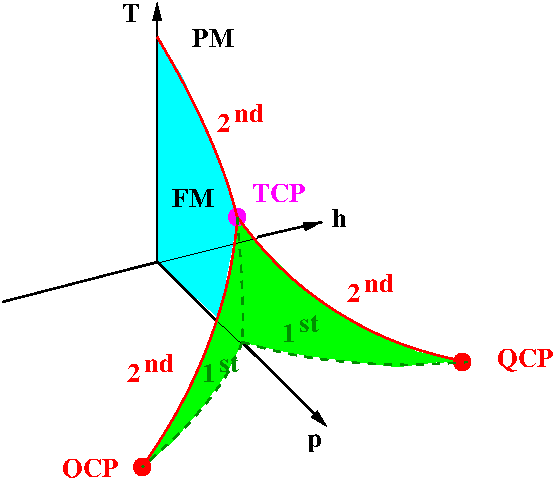
Figure 1: Schematic phase diagram in the space spanned by temperature ($T$), hydrostatic pressure ($p$), and magnetic field ($h$). Shown are the FM and PM phases, the tricritical point (TCP), and the two quantum critical points (QCP). Solid and dashed lines denote second- and first-order transitions, respectively. The tricritical wings emerging from the TCP are surfaces of first-order transitions.

III Discussion

The mechanism we have described that leads to a first-order quantum ferromagnetic transition is very general: It is a universal long-wavelength effect that depends only on the presence of conduction electrons that form a Fermi liquid. It thus is valid for any metallic ferromagnet with a Fermi surface. A comparison with other theoretical analyses that have come to different conclusions for the special case of a Kondo lattice is therefore called for, and we start our discussion with this.

Mean-field approximations on Eqs. (1) have been used to develop a Stoner-like theory of ferromagnetism on a Kondo lattice Yu. Irkhin and Katsnelson (1990); Perkins et al. (2007); Yu. Irkhin (2014). As one would expect within such an approach, it generically yields a transition that is continuous with mean-field critical exponents, although the transition may be first order due to special features in the density of states Yu. Irkhin and Katsnelson (1990); Yu. Irkhin (2014). Later, Yamamoto and Si Yamamoto and Si (2010) used a combination of field theoretic and RG methods in an attempt to understand the fate of the Kondo screening in the ferromagnetic phase. For an antiferromagnetic Kondo coupling $J>0$, and for $J\ll|I|$, they concluded that the Kondo coupling flows to zero, the Kondo screening in the ferromagnetic phase breaks down, and the system has a small Fermi surface. While their focus was on the stable fixed point that describes the ferromagnetic phase, their results imply that the ferromagnetic quantum phase transition is second order. That is, the RG treatment does not change the order of the phase transition compared to the generalized Stoner theory of Ref. Perkins et al. (2007). Two related points are: (1) The analysis of Ref. Yamamoto and Si (2010) does not yield the nonanalytic wave-number dependence found in Ref. Chubukov et al. (2004) for a closely related model. (2) It finds a linear magnetization dependence for the spin-wave stiffness coefficient $D(m)$ in the magnon dispersion relation $\Omega=D(m){\bm{k}}^{2}$, whereas Ref. Belitz et al. (1998) found a nonanalytic $m$-dependence of $D$ for a quantum nonlinear sigma model. All of these effects, as well as the nonanalytic field dependence of the spin susceptibility of a Fermi liquid, Eq. (14), have the same origin, and lead to a first-order quantum ferromagnetic transition as discussed in Sec. II. These discrepancies can be traced back to the fact that the starting action of Ref. Yamamoto and Si (2010) does not contain any interactions for the conduction electrons, and the latter are responsible for the nonanalyticities that in turn lead to the first-order transition. In principle, a complete RG analysis will generate an electronic interaction, via an exchange of excitations in the local-moment system to which the conduction electrons are coupled, even if none was included in the bare action. However, this requires the consideration of terms of higher-loop order than were kept in Ref. Yamamoto and Si (2010). The fluctuations that cause the first-order transition discussed in Sec. II were thus effectively not considered.

We conclude with a number of additional remarks:

1. Our conclusion that the ferromagnetic quantum phase transition in clean heavy-fermion or Kondo-lattice systems is first order is in agreement with experimental results. Examples include UGe₂ Huxley et al. (2001, 2007), URhGe Aoki et al. (2011); Huxley et al. (2007), and UCoGe Aoki et al. (2011); Hattori et al. (2010).

2. As already mentioned in Sec. II.2, there are a number of dynamic processes in the Kondo-lattice problem, and corresponding frqeuency-dependent terms in the action. One is the Berry-phase term that describes the Bloch precession of the local moments, Eq. (4). It is physically obvious, although not commonly appreciated, that such a term must also exist in the action for an itinerant ferromagnet, in which case it is generated by the dynamics of the conduction electrons. In addition, there is a term describing relaxation processes that do not become slow in the limit of small wave numbers. At a continuous quantum phase transition, all three of these terms are irrelevant compared to the Landau-damping term given by Eq. (5).

3. It follows from thermodynamic considerations alone, namely, from various Clapeyron-Clausius relations, that the tricritical wings shown in Fig. 1 are perpendicular to the $T=0$ plane, but not perpendicular to the $p$-axis and point in the direction of the paramagnetic phase Kirkpatrick and Belitz (2015). These features, as well as the overall structure of the phase diagram, are in excellent agreement with experimental observations Brando et al. .

   

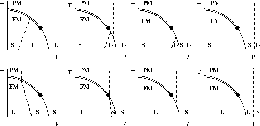
   Figure 2: Possible temperature - pressure ($T$-$p$) phase diagrams for systems with a small (first row) or large (second row) Fermi surface deep inside the ferromagnetic (FM) phase. Double and single solids lines represent continuous and first-order transitions, respectively, from a paramagnetic (PM) phase to a FM one, separated by a tricritical point (dot). Dashed lines represent the hybridization temperature whose pressure dependence has been neglected for simplicity. S and L indicate regions of small and large Fermi surfaces, respectively.

4. Quenched non-magnetic disorder changes the nature of the fermionic soft modes from ballistic to diffusive. More importantly, it changes the sign of the non-analytic term in Eqs. (14) and (15). This is because the interplay of electron-electron interactions and quenched disorder enhances the electronic spin susceptibility compared to the Pauli susceptibility Altshuler and Aronov (1984); Finkelstein (1983). That is, the combined disorder and interaction fluctuations increase the zero-field susceptibility. A magnetic field again suppresses the fluctuations, and hence the sign of the nonanalyticity in $\chi_{h}\to 0)$ changes compared to Eq. (14):

   $$\chi(h\to 0)=\chi(0)-{\tilde{a}}_{d}\,h^{(d-2)/2}\qquad(2<d<4)\ ,$$ (16)

   with ${\tilde{a}}_{d}>0$. The changed exponent reflects the diffusive nature of the soft modes. As a result, the transition within the renormalized mean-field theory is second order with non-mean-field exponents. The evolution of the phase diagram with increasing disorder strength has been discussed in Ref. Sang et al. (2014), and the asymptotic and pre-asymptotic critical behavior in Ref.  Kirkpatrick and Belitz (2014).

5. For an antiferromagnetic Kondo coupling $J$, the existence or otherwise of Kondo screening in the FM phase needs to be reconsidered. The scale dimension of the Kondo coupling, which determines the answer, depends on the dynamical scale dimension of the order-parameter field Yamamoto and Si (2010), which in turn depends on the same physics that determines the order of the phase transition. The RG analysis of Ref. Yamamoto and Si (2010) concluded that deep inside the FM phase the Kondo screening generically breaks down, i.e., the Fermi surface is small. For FM systems that are driven paramagnetic by the application of pressure, such as UGe₂, this would imply that there is a hybridization transition from a small Fermi surface to a large one with increasing pressure. Assuming that an applied field, or a spontaneous magnetization, favors a large Fermi surface at least in a range of fields, as is the case in the antiferromagnetic heavy-fermion metal CeRhIn₅ Jiao et al. (2015) (see also the phenomenological theory of Ref. Yang and Pines (2014)), this suggests possible phase diagrams as shown in the first row of Fig. 2. However, for antiferromagnetic Kondo lattices it is known that hydrostatic pressure can either favor or suppress hybridization in different materials Yang and Pines (2014), and for UGe₂ there is some experimental evidence for a large Fermi surface deep inside the FM phase and a small one close to the first-order transition Huxley et al. (2003). Possible phase diagrams for this case are shown in the second row of Fig. 2. If a field or magnetization favors a small Fermi surface, as must be the case at least in very strong fields and is observed in, e.g., the antiferromagnet CeRu₂Si₂ van der Meulen et al. (1991) (see also, e.g., Refs. Belitskii and Goltsev (1989); Kusminskyi et al. (2008)), the position and direction of the dashed line within the FM phase in Fig. 2 will change in obvious ways. We also note that the hybridization transition is a true phase transition only at $T=0$, and a crossover at $T>0$. However, even a crossover could trigger a metamagnetic transition with a sharp discontinuity in the magnetization. This raises the possibility that the FM2-to-FM1 metamagnetic transition observed in UGe₂ is a signature of the hybridization transition Huxley et al. (2003). The critical behavior at the critical point where the line of first-order metamagnetic transitions ends has been analyzed in Ref. Millis et al. (2002).

6. If the Fermi surface deep inside the FM phase is large (small) and if a magnetization enhances (suppresses) hybridization, then there will be a whole region of parameter values for which the magnetic transition and the hybridization transition coincide, as can be seen from the third panel in the second row of Fig. 2. In the case of a first-order magnetic transition the two transitions can thus coincide generically, whereas for a second-order transition this can happen only for a set of parameter values that is of measure zero.