Dimension Reduction for Gaussian Process Emulation: An Application to the Influence of Bathymetry on Tsunami Heights

Xiaoyu Liu and Serge Guillas
Department of Statistical Science, University College London
Abstract

High accuracy complex computer models, also called simulators, require large resources in time and memory to produce realistic results. Statistical emulators are computationally cheap approximations of such simulators. They can be built to replace simulators for various purposes, such as the propagation of uncertainties from inputs to outputs or the calibration of some internal parameters against observations. However, when the input space is of high dimension, the construction of an emulator can become prohibitively expensive. In this paper, we introduce a joint framework merging emulation with dimension reduction in order to overcome this hurdle. The gradient-based kernel dimension reduction technique is chosen due to its ability to drastically decrease dimensionality with little loss in information. The Gaussian process emulation technique is combined with this dimension reduction approach. Theoretical properties of the approximation are explored. Our proposed approach provides an answer to the dimension reduction issue in emulation for a wide range of simulation problems that cannot be tackled using existing methods. The efficiency and accuracy of the proposed framework is demonstrated theoretically, and compared with other methods on an elliptic partial differential equation (PDE) problem. We finally present a realistic application to tsunami modeling. The uncertainties in the bathymetry (seafloor elevation) are modeled as high-dimensional realizations of a spatial process using a geostatistical approach. Our dimension-reduced emulation enables us to compute the impact of these uncertainties on resulting possible tsunami wave heights near-shore and on-shore. Considering an uncertain earthquake source, we observe a significant increase in the spread of uncertainties in the tsunami heights due to the contribution of the bathymetry uncertainties to the overall uncertainty budget. These results highlight the need to include the effect of uncertainties in the bathymetry in tsunami early warnings and risk assessments.


Keywords: Dimension reduction, Gaussian process, statistical emulation, uncertainty quantification

1 Introduction

Simulators are widely employed to reproduce physical processes and explore their behavior, in fields such as fluid dynamics or climate modeling. To characterize the impact of the uncertainties in the boundary conditions or the parameterizations of the underlying physical processes, a sufficient number of simulations are required. However, when the simulators are computationally expensive, as it is the case for high accuracy simulations, the task can become extremely costly or even prohibitive. One prevailing way to overcome this hurdle is to construct statistical surrogates, namely emulators, to approximate the computer simulators in a probabilistic way [29]. Emulators are trained on a relatively small number of well chosen simulations, i.e. a design of computer experiments. Outputs at any input can be predicted at little computational cost with emulators. One can then employ emulators for any subsequent purposes such as uncertainty propagation, sensitivity analysis and calibration.

With high-dimensional inputs, say beyond 20 dimensions (usually in the hundreds or thousands), a large design is usually required to explore the input space, typically in the order of 10 times the number of dimensions, for a reasonable level of approximation. One would face serious computational problems since the original simulator cannot be run many times or is very expensive to run. Advanced designs such as Latin Hypercubes or new sequential designs [4] that are more efficient than Latin Hypercubes only partially alleviate the issue. As a result, methods that adequately reduce the dimension of the input space are required, as high-dimensional inputs are often present in computer models, e.g. as boundary conditions like the bathymetry (i.e. seafloor elevation) in tsunami modeling. Some approaches ignore high-dimensional inputs and add stochastic terms to account for their contribution [19, 25]. These methods are easy to implement and effective in some applications. However, repeated simulations at the same input parameters that are encoded in the emulation are often required to estimate the variability due to those parameters that are ignored. The variability estimates are often restricted to the second moments, and the input-output relationships over the ignored inputs are not clear. Constantine et al. [6] proposed to find rotations of the input space with the strongest variability in the gradients of the simulators and constructed a response surface on such a low-dimensional active subspace. This Active Subspace (AS) approach has been demonstrated to be effective theoretically and numerically. Constantine and Gleich [5] studied further the properties of the Monte Carlo approximation of the subspace. However, this method requires the calculation of a sufficient number of gradients explicitly, which unfortunately prevents its use in many applications. The gradients are often unavailable in many realistic simulators, and typically intractable for systems of mixed PDEs or multi-physics simulations. Even in the rare situations where gradients are computable numerically, the computational cost of obtaining them could be prohibitive.

The concept of active subspace is closely related to the sufficient dimension reduction (SDR) [7, 9] and effective dimension reduction (EDR) [22] in the statistical community. Given an explanatory variable ๐—โˆˆโ„m๐—superscriptโ„๐‘š\mathbf{X}\in\mathbb{R}^{m} (input) and response variable Y๐‘ŒY (output), the aim of SDR (or EDR) is to find the directions in the subspace of ๐—๐—\mathbf{X} that contain sufficient information about the response for statistical inference. More specifically, a SDR Rโ€‹(๐—)โˆˆโ„d๐‘…๐—superscriptโ„๐‘‘R(\mathbf{X})\in\mathbb{R}^{d} where d<m๐‘‘๐‘šd<m satisfies pโ€‹(Y|๐—)=p~โ€‹(Y|Rโ€‹(๐—)),๐‘conditional๐‘Œ๐—~๐‘conditional๐‘Œ๐‘…๐—p(Y|\mathbf{X})=\tilde{p}(Y|R(\mathbf{X})), where pโ€‹(Y|๐—)๐‘conditional๐‘Œ๐—p(Y|\mathbf{X}) and p~โ€‹(Y|Rโ€‹(๐—))~๐‘conditional๐‘Œ๐‘…๐—\tilde{p}(Y|R(\mathbf{X})) are conditional probability density functions with respect to ๐—๐—\mathbf{X} and Rโ€‹(๐—)๐‘…๐—R(\mathbf{X}) respectively. The EDR approach aims to specifically find a linear projection matrix ๐๐\mathbf{B} onto a d๐‘‘d-dimensional subspace (d<m)๐‘‘๐‘š(d<m) such that ๐Tโ€‹๐=๐ˆdsuperscript๐๐‘‡๐subscript๐ˆ๐‘‘\mathbf{B}^{T}\mathbf{B}=\mathbf{I}_{d} and

pโ€‹(Y|๐—)=p~โ€‹(Y|๐Tโ€‹๐—)โ€‹or equivalentlyโ€‹YโŸ‚X|๐Tโ€‹X.๐‘conditional๐‘Œ๐—~๐‘conditional๐‘Œsuperscript๐๐‘‡๐—or equivalently๐‘Œperpendicular-toconditional๐‘‹superscript๐๐‘‡๐‘‹p(Y|\mathbf{X})=\tilde{p}(Y|\mathbf{B}^{T}\mathbf{X})~{}~{}~{}\textrm{or equivalently}~{}~{}~{}Y\perp X|\mathbf{B}^{T}X. (1)

Several methods have been developed to find SDR including nonparametric approaches such as sliced inverse regression (SIR) [22], minimum average variance estimation (MAVE) [30], and parametric approaches like principal fitted components (PFC) [8, 10]. In this paper, we adopt the gradient-based kernel dimension reduction (gKDR) [15] to construct low-dimensional approximations to the simulators. The gKDR approach does not require any strong assumptions on the variables and distributions. The response variable can be of arbitrary type: continuous or discrete, univariate or multivariate. Unlike the active subspace method, gradients are not required to be computed explicitly but are estimated non-parametrically and implicitly using stable kernel methods. Our proposed approach therefore provides an answer to the dimension reduction issue in emulation for a wide range of problems that cannot be tackled using existing methods at the moment. Moreover, the gKDR approach ends up with an eigen-problem without any needs of elaborate numerical optimization and thus can be applied to large and high-dimensional problems.

We introduce a joint framework to approximate the high-dimensional simulators by combining statistical emulators with the gKDR approach. Deterministic simulators are considered here, however the framework could potentially be applied to stochastic simulators, with additional treatments to the stochastic effect in the emulation, see e.g. [18]. Throughout this paper, the mainstream Gaussian process (GP) emulators are employed for illustration. But the general framework and most of the results would potentially hold for other emulation techniques.

The paper is organized as follows. Sectionย 2 and 3 review GP emulation and the gKDR approach respectively. In Sectionย 4, a joint framework of dimension reduction combined with emulation is proposed and some theoretical properties are established. Sectionย 5 contains the numerical experiments on an elliptic PDE and an application to the propagation of uncertainties in the bathymetry to tsunami wave heights, as well as comparison with alternative methods. Sectionย 6 consists of some conclusive discussion.

2 Gaussian process emulation

A Gaussian process is a collection of random variables such that any finite subset of these variables follow a joint Gaussian distribution [27]. It is widely used in various scientific fields. Here we briefly review some basics of its application in statistical emulation.

A deterministic simulator with multivariate input ๐—=(x1,โ€ฆ,xm)Tโˆˆโ„m๐—superscriptsubscript๐‘ฅ1โ€ฆsubscript๐‘ฅ๐‘š๐‘‡superscriptโ„๐‘š\mathbf{X}=(x_{1},...,x_{m})^{T}\in\mathbb{R}^{m} and univariate output Yโˆˆโ„๐‘Œโ„Y\in\mathbb{R} can be represented as Y=fโ€‹(๐—)๐‘Œ๐‘“๐—Y=f(\mathbf{X}). The GP emulator assumes that the simulator output Y=fโ€‹(๐—)๐‘Œ๐‘“๐—Y=f(\mathbf{X}) can be modeled with a Gaussian process. It is commonly assumed that the mean can be written as Eโก(Y)=mโ€‹(๐—)=๐กTโ€‹(๐—)โ€‹๐œทE๐‘Œ๐‘š๐—superscript๐ก๐‘‡๐—๐œท\operatorname{E}(Y)=m(\mathbf{X})=\mathbf{h}^{T}(\mathbf{X})\boldsymbol{\beta}, where ๐กโ€‹(๐—)๐ก๐—\mathbf{h}(\mathbf{X}) is a q๐‘žq-vector of pre-defined regression functions and the coefficients ๐œทโˆˆโ„q๐œทsuperscriptโ„๐‘ž\boldsymbol{\beta}\in\mathbb{R}^{q}. In practice, a constant or linear form for the regression functions would perform well. The covariance between two simulator outputs Y=fโ€‹(๐—)๐‘Œ๐‘“๐—Y=f(\mathbf{X}) and Yโ€ฒ=fโ€‹(๐—โ€ฒ)superscript๐‘Œโ€ฒ๐‘“superscript๐—โ€ฒY^{\prime}=f(\mathbf{X}^{\prime}) is usually represented as Covโก(Y,Yโ€ฒ)=kโ€‹(๐—,๐—โ€ฒ)=ฯƒ2โ€‹cโ€‹(๐—,๐—โ€ฒ)Cov๐‘Œsuperscript๐‘Œโ€ฒ๐‘˜๐—superscript๐—โ€ฒsuperscript๐œŽ2๐‘๐—superscript๐—โ€ฒ\operatorname{Cov}(Y,Y^{\prime})=k(\mathbf{X},\mathbf{X}^{\prime})=\sigma^{2}c(\mathbf{X},\mathbf{X}^{\prime}), where the positive scalar parameter ฯƒ2superscript๐œŽ2\sigma^{2} is the process variance and cโ€‹(๐—,๐—โ€ฒ)๐‘๐—superscript๐—โ€ฒc(\mathbf{X},\mathbf{X}^{\prime}) is the correlation function. One common choice for the correlation function is the squared-exponential correlation cโ€‹(๐—,๐—โ€ฒ)=โˆi=1mexpโก(โˆ’(xiโˆ’xiโ€ฒ)2/ฮดi2),๐‘๐—superscript๐—โ€ฒsuperscriptsubscriptproduct๐‘–1๐‘šsuperscriptsubscript๐‘ฅ๐‘–superscriptsubscript๐‘ฅ๐‘–โ€ฒ2superscriptsubscript๐›ฟ๐‘–2c(\mathbf{X},\mathbf{X}^{\prime})=\prod_{i=1}^{m}\exp\left(-(x_{i}-x_{i}^{\prime})^{2}/\delta_{i}^{2}\right), where ๐œน=(ฮด1,โ€ฆ,ฮดm)Tโˆˆ(0,โˆž)m๐œนsuperscriptsubscript๐›ฟ1โ€ฆsubscript๐›ฟ๐‘š๐‘‡superscript0๐‘š\boldsymbol{\delta}=(\delta_{1},...,\delta_{m})^{T}\in(0,\infty)^{m} controls the correlation lengths.

Suppose that the simulator is run at n๐‘›n inputs ๐—1,โ€ฆ,๐—nsubscript๐—1โ€ฆsubscript๐—๐‘›\mathbf{X}_{1},...,\mathbf{X}_{n} and the outputs are Y1,โ€ฆ,Ynsubscript๐‘Œ1โ€ฆsubscript๐‘Œ๐‘›Y_{1},...,Y_{n} respectively. We may need to impose a prior for the parameter ๐œท๐œท\boldsymbol{\beta} in the mean function mโ€‹(๐—)=๐กTโ€‹(๐—)โ€‹๐œท๐‘š๐—superscript๐ก๐‘‡๐—๐œทm(\mathbf{X})=\mathbf{h}^{T}(\mathbf{X})\boldsymbol{\beta}. One of the popular choices is a Gaussian prior, ๐œทโˆผNโก(๐›,๐•)similar-to๐œทN๐›๐•\boldsymbol{\beta}\sim\operatorname{N}(\mathbf{b},\mathbf{V}), which forms a conjugate prior with the GP likelihood. At any nโˆ—superscript๐‘›n^{*} desired inputs ๐—1โˆ—,๐—2โˆ—,โ€ฆ,๐—nโˆ—โˆ—superscriptsubscript๐—1superscriptsubscript๐—2โ€ฆsuperscriptsubscript๐—superscript๐‘›\mathbf{X}_{1}^{*},\mathbf{X}_{2}^{*},...,\mathbf{X}_{n^{*}}^{*}, the respective outputs are denoted by Y1โˆ—,Y2โˆ—,โ€ฆ,Ynโˆ—โˆ—superscriptsubscript๐‘Œ1superscriptsubscript๐‘Œ2โ€ฆsuperscriptsubscript๐‘Œsuperscript๐‘›Y_{1}^{*},Y_{2}^{*},...,Y_{n^{*}}^{*}. Then letting ๐‡=(๐กโ€‹(๐—1),โ€ฆ,๐กโ€‹(๐—n))๐‡๐กsubscript๐—1โ€ฆ๐กsubscript๐—๐‘›\mathbf{H}=(\mathbf{h}(\mathbf{X}_{1}),...,\mathbf{h}(\mathbf{X}_{n})) and ๐‡โˆ—=(๐กโ€‹(๐—1โˆ—),โ€ฆ,๐กโ€‹(๐—nโˆ—))superscript๐‡๐กsuperscriptsubscript๐—1โ€ฆ๐กsuperscriptsubscript๐—๐‘›\mathbf{H}^{*}=(\mathbf{h}(\mathbf{X}_{1}^{*}),...,\mathbf{h}(\mathbf{X}_{n}^{*})), the predictive process of ๐˜โˆ—superscript๐˜\mathbf{Y}^{*} (also known as kriging prediction) given the observed data and the covariance function is

๐˜โˆ—|๐˜,kโ€‹(โ‹…,โ‹…;๐œฝ)โˆผNโก(๐ฆ^โˆ—,๐šบ^โˆ—),similar-toconditionalsuperscript๐˜๐˜๐‘˜โ‹…โ‹…๐œฝNsuperscript^๐ฆsuperscript^๐šบ\mathbf{Y}^{*}|\mathbf{Y},k(\cdot,\cdot;\boldsymbol{\theta})\sim\operatorname{N}(\hat{\mathbf{m}}^{*},\hat{\boldsymbol{\Sigma}}^{*}), (2)

with

๐ฆ^โˆ—=๐‡โˆ—Tโ€‹๐œท^+๐Šโˆ—โ€‹๐Šโˆ’1โ€‹(๐˜โˆ’๐‡Tโ€‹๐œท^),superscript^๐ฆsuperscript๐‡absent๐‘‡^๐œทsubscript๐Šsuperscript๐Š1๐˜superscript๐‡๐‘‡^๐œท\hat{\mathbf{m}}^{*}=\mathbf{H}^{*T}\hat{\boldsymbol{\beta}}+\mathbf{K}_{*}\mathbf{K}^{-1}(\mathbf{Y}-\mathbf{H}^{T}\hat{\boldsymbol{\beta}}), (3)

and

๐šบ^โˆ—=๐Šโˆ—โˆ—+๐Tโ€‹(๐•โˆ’1+๐‡๐Šโˆ’1โ€‹๐‡T)โˆ’1โ€‹๐,superscript^๐šบsubscript๐Šabsentsuperscript๐๐‘‡superscriptsuperscript๐•1superscript๐‡๐Š1superscript๐‡๐‘‡1๐\hat{\boldsymbol{\Sigma}}^{*}=\mathbf{K}_{**}+\mathbf{P}^{T}(\mathbf{V}^{-1}+\mathbf{H}\mathbf{K}^{-1}\mathbf{H}^{T})^{-1}\mathbf{P}, (4)

where ๐œฝ๐œฝ\boldsymbol{\theta} represents the hyperparameters from the covariance function, ๐Š๐Š\mathbf{K}, ๐Šโˆ—subscript๐Š\mathbf{K}_{*} and ๐Šโˆ—โˆ—subscript๐Šabsent\mathbf{K}_{**} are nร—n๐‘›๐‘›n\times n, nโˆ—ร—nsuperscript๐‘›๐‘›n^{*}\times n and nโˆ—ร—nโˆ—superscript๐‘›superscript๐‘›n^{*}\times n^{*} matrices respectively with the associated (i,j)๐‘–๐‘—(i,j)-th entry as ๐Šโ€‹(i,j)=kโ€‹(๐—i,๐—j)๐Š๐‘–๐‘—๐‘˜subscript๐—๐‘–subscript๐—๐‘—\mathbf{K}(i,j)=k(\mathbf{X}_{i},\mathbf{X}_{j}), ๐Šโˆ—โ€‹(i,j)=kโ€‹(๐—iโˆ—,๐—j)subscript๐Š๐‘–๐‘—๐‘˜superscriptsubscript๐—๐‘–subscript๐—๐‘—\mathbf{K}_{*}(i,j)=k(\mathbf{X}_{i}^{*},\mathbf{X}_{j}) and ๐Šโˆ—โˆ—โ€‹(i,j)=kโ€‹(๐—iโˆ—,๐—jโˆ—)subscript๐Šabsent๐‘–๐‘—๐‘˜superscriptsubscript๐—๐‘–superscriptsubscript๐—๐‘—\mathbf{K}_{**}(i,j)=k(\mathbf{X}_{i}^{*},\mathbf{X}_{j}^{*}), ๐=๐‡โˆ—โˆ’๐‡๐Šโˆ’1โ€‹๐Šโˆ—T๐superscript๐‡superscript๐‡๐Š1superscriptsubscript๐Š๐‘‡\mathbf{P}=\mathbf{H}^{*}-\mathbf{H}\mathbf{K}^{-1}\mathbf{K}_{*}^{T} and ๐œท^=(๐•โˆ’1+๐‡๐Šโˆ’1โ€‹๐‡T)โˆ’1โ€‹(๐‡๐Šโˆ’1โ€‹๐˜+๐•โˆ’1โ€‹๐›)^๐œทsuperscriptsuperscript๐•1superscript๐‡๐Š1superscript๐‡๐‘‡1superscript๐‡๐Š1๐˜superscript๐•1๐›\hat{\boldsymbol{\beta}}=(\mathbf{V}^{-1}+\mathbf{H}\mathbf{K}^{-1}\mathbf{H}^{T})^{-1}(\mathbf{H}\mathbf{K}^{-1}\mathbf{Y}+\mathbf{V}^{-1}\mathbf{b}).

We can see that the output at any desired input predicted using a GP emulator is a distribution rather than a single value. This could be used to estimate the uncertainty introduced into the prediction with emulator and to evaluate the confidence about the prediction. However, the hyperparameters ๐œฝ๐œฝ\boldsymbol{\theta} is usually unknown and needs to be specified properly. It is possible to make a fully Bayesian inference with appropriate prior ฯ€โ€‹(๐œฝ)๐œ‹๐œฝ\pi(\boldsymbol{\theta}). But this usually requires costly MCMC approach for the analytically intractable posterior. In practice, a computationally cheap alternative is often employed by specifying the hyperparameters ๐œฝ๐œฝ\boldsymbol{\theta} at the most probable values. This could be done by maximizing the marginal likelihood,

Lโ€‹(๐œฝ)=logโกpโ€‹(๐˜|๐›,๐•)=โˆ’12โ€‹(๐‡Tโ€‹๐›โˆ’๐˜)Tโ€‹(๐Š+๐‡Tโ€‹๐•๐‡)โˆ’1โ€‹(๐‡Tโ€‹๐›โˆ’๐˜)โˆ’12โ€‹logโก|๐Š+๐‡Tโ€‹๐•๐‡|โˆ’n2โ€‹logโก2โ€‹ฯ€.๐ฟ๐œฝ๐‘conditional๐˜๐›๐•12superscriptsuperscript๐‡๐‘‡๐›๐˜๐‘‡superscript๐Šsuperscript๐‡๐‘‡๐•๐‡1superscript๐‡๐‘‡๐›๐˜12๐Šsuperscript๐‡๐‘‡๐•๐‡๐‘›22๐œ‹\displaystyle\begin{split}L(\boldsymbol{\theta})&=\log p(\mathbf{Y}|\mathbf{b},\mathbf{V})\\ &=-\frac{1}{2}(\mathbf{H}^{T}\mathbf{b}-\mathbf{Y})^{T}(\mathbf{K}+\mathbf{H}^{T}\mathbf{V}\mathbf{H})^{-1}(\mathbf{H}^{T}\mathbf{b}-\mathbf{Y})-\frac{1}{2}\log|\mathbf{K}+\mathbf{H}^{T}\mathbf{V}\mathbf{H}|-\frac{n}{2}\log 2\pi.\end{split} (5)

Then the prediction can be completed by plugging in ๐œฝ^=argmax๐œฝโกLโ€‹(๐œฝ)^๐œฝsubscriptargmax๐œฝ๐ฟ๐œฝ\hat{\boldsymbol{\theta}}=\operatorname{argmax}_{\boldsymbol{\theta}}L(\boldsymbol{\theta}).

Usually there is no sufficient information about the parameter ๐œท๐œท\boldsymbol{\beta}, hence a vague prior can be imposed by letting ๐•โˆ’1โ†’๐Žโ†’superscript๐•1๐Ž\mathbf{V}^{-1}\rightarrow\mathbf{O} and ๐›=๐ŸŽ๐›0\mathbf{b}=\mathbf{0}, where ๐Ž๐Ž\mathbf{O} is the matrix of zeros. In this case, the conditional mean and covariance of the predictive process are respectively

๐ฆ^โˆ—=๐‡โˆ—Tโ€‹๐œท^+๐Šโˆ—โ€‹๐Šโˆ’1โ€‹(๐˜โˆ’๐‡โ€‹๐œท^),superscript^๐ฆsuperscript๐‡absent๐‘‡^๐œทsubscript๐Šsuperscript๐Š1๐˜๐‡^๐œท\hat{\mathbf{m}}^{*}=\mathbf{H}^{*T}\hat{\boldsymbol{\beta}}+\mathbf{K}_{*}\mathbf{K}^{-1}(\mathbf{Y}-\mathbf{H}\hat{\boldsymbol{\beta}}), (6)

and

๐šบ^โˆ—=๐Šโˆ—โˆ—+๐Tโ€‹(๐‡๐Šโˆ’1โ€‹๐‡T)โˆ’1โ€‹๐,superscript^๐šบsubscript๐Šabsentsuperscript๐๐‘‡superscriptsuperscript๐‡๐Š1superscript๐‡๐‘‡1๐\hat{\boldsymbol{\Sigma}}^{*}=\mathbf{K}_{**}+\mathbf{P}^{T}(\mathbf{H}\mathbf{K}^{-1}\mathbf{H}^{T})^{-1}\mathbf{P}, (7)

where ๐œท^=(๐‡๐Šโˆ’1โ€‹๐‡T)โˆ’1โ€‹๐‡๐Šโˆ’1โ€‹๐˜^๐œทsuperscriptsuperscript๐‡๐Š1superscript๐‡๐‘‡1superscript๐‡๐Š1๐˜\hat{\boldsymbol{\beta}}=(\mathbf{H}\mathbf{K}^{-1}\mathbf{H}^{T})^{-1}\mathbf{H}\mathbf{K}^{-1}\mathbf{Y}. This is closely related to the t๐‘กt-process [26] when a weak prior for (๐œท,ฯƒ2,๐œน)๐œทsuperscript๐œŽ2๐œน(\boldsymbol{\beta},\sigma^{2},\boldsymbol{\delta}) that ฯ€โ€‹(๐œท,ฯƒ2,๐œน)โˆฯƒโˆ’2โ€‹ฯ€๐œนโ€‹(๐œน)proportional-to๐œ‹๐œทsuperscript๐œŽ2๐œนsuperscript๐œŽ2subscript๐œ‹๐œน๐œน\pi(\boldsymbol{\beta},\sigma^{2},\boldsymbol{\delta})\propto\sigma^{-2}\pi_{\boldsymbol{\delta}}(\boldsymbol{\delta}) is assumed with the mean function mโ€‹(โ‹…)=๐กTโ€‹(โ‹…)โ€‹๐œท๐‘šโ‹…superscript๐ก๐‘‡โ‹…๐œทm(\cdot)=\mathbf{h}^{T}(\cdot)\boldsymbol{\beta} and the covariance function kโ€‹(โ‹…,โ‹…)=ฯƒ2โ€‹cโ€‹(โ‹…,โ‹…;๐œน)๐‘˜โ‹…โ‹…superscript๐œŽ2๐‘โ‹…โ‹…๐œนk(\cdot,\cdot)=\sigma^{2}c(\cdot,\cdot;\boldsymbol{\delta}), where ๐œน๐œน\boldsymbol{\delta} contains the parameters in the correlation function cโ€‹(โ‹…,โ‹…)๐‘โ‹…โ‹…c(\cdot,\cdot).

When kโ€‹(๐—,๐—โ€ฒ)=ฯƒ2โ€‹cโ€‹(๐—,๐—โ€ฒ)๐‘˜๐—superscript๐—โ€ฒsuperscript๐œŽ2๐‘๐—superscript๐—โ€ฒk(\mathbf{X},\mathbf{X}^{\prime})=\sigma^{2}c(\mathbf{X},\mathbf{X}^{\prime}) is used with a continuous correlation function, such as the squared-exponential correlation, the emulator interpolates through the training data, i.e. m^โ€‹(๐—i)=Yi^๐‘šsubscript๐—๐‘–subscript๐‘Œ๐‘–\hat{m}(\mathbf{X}_{i})=Y_{i} and v^โ€‹(๐—i)=0^๐‘ฃsubscript๐—๐‘–0\hat{v}(\mathbf{X}_{i})=0 at the training points {๐—i}i=1nsuperscriptsubscriptsubscript๐—๐‘–๐‘–1๐‘›\{\mathbf{X}_{i}\}_{i=1}^{n}. When a nugget term is included, this is no longer true. A nugget term can be included, e.g. to mitigate numerical instabilities or account for the stochastic terms in simulations [3]. The correlation function cโ€‹(๐—,๐—โ€ฒ)๐‘๐—superscript๐—โ€ฒc(\mathbf{X},\mathbf{X}^{\prime}) can be extended with the addition of a nugget as c~โ€‹(๐—,๐—โ€ฒ)=ฮฝโ€‹I๐—=๐—โ€ฒ+(1โˆ’ฮฝ)โ€‹cโ€‹(๐—,๐—โ€ฒ),~๐‘๐—superscript๐—โ€ฒ๐œˆsubscript๐ผ๐—superscript๐—โ€ฒ1๐œˆ๐‘๐—superscript๐—โ€ฒ\tilde{c}(\mathbf{X},\mathbf{X}^{\prime})=\nu I_{\mathbf{X}=\mathbf{X}^{\prime}}+(1-\nu)c(\mathbf{X},\mathbf{X}^{\prime}), where ฮฝ>0๐œˆ0\nu>0 is the nugget term, and I๐—=๐—โ€ฒsubscript๐ผ๐—superscript๐—โ€ฒI_{\mathbf{X}=\mathbf{X}^{\prime}} is the indicator function that takes 111 if ๐—=๐—โ€ฒ๐—superscript๐—โ€ฒ\mathbf{X}=\mathbf{X}^{\prime} and 00 otherwise. The associated correlation matrix is ๐Š~=(1โˆ’ฮฝ)โ€‹๐Š+ฮฝโ€‹๐ˆ~๐Š1๐œˆ๐Š๐œˆ๐ˆ\tilde{\mathbf{K}}=(1-\nu)\mathbf{K}+\nu\mathbf{I}, where ๐ˆ๐ˆ\mathbf{I} is the identity matrix.

In practice, the error in the prediction of GP emulator depends on the number of training data points. As there are more and more training data points, the GP emulator will be expected to recover the simulator. There are several theoretical results on how well the GP emulator f^^๐‘“\hat{f} can approximate the simulator f๐‘“f in the literature. For example, given n๐‘›n training samples that are quasi-uniformly distributed on ฮฉโŠ‚โ„dฮฉsuperscriptโ„๐‘‘\Omega\subset\mathbb{R}^{d}, the error can be bounded [13] as โ€–fโˆ’f^โ€–โˆžโ‰คCdโ€‹nโˆ’p/dโ€‹โ€–fโ€–โ„‹subscriptnorm๐‘“^๐‘“subscript๐ถ๐‘‘superscript๐‘›๐‘๐‘‘subscriptnorm๐‘“โ„‹\|f-\hat{f}\|_{\infty}\leq C_{d}n^{-p/d}\|f\|_{\mathcal{H}} for any f๐‘“f in some function space โ„‹โ„‹\mathcal{H} over ฮฉฮฉ\Omega, typically a Hilbert space, where p๐‘p controls the smoothness of the function and Cdsubscript๐ถ๐‘‘C_{d} is a constant depending on the dimension d๐‘‘d. This result suggests that f^^๐‘“\hat{f} provides arbitrarily high approximation order when p=โˆž๐‘p=\infty, i.e. f๐‘“f is infinitely smooth. However, this rate decreases as the dimension increases and the constant Cdsubscript๐ถ๐‘‘C_{d} also grows with d๐‘‘d. Hence, the approximation deteriorates in very high dimensions. This implies that more evaluations of the simulator are required to train an accurate emulator when the number of input parameters d๐‘‘d increases and the associated computational cost of constructing an emulator could increase dramatically as a result. Therefore, it is desirable to reduce the dimension of the problem from the perspectives of both accuracy and efficiency.

3 Gradient-based kernel dimension reduction

For a set ฮฉฮฉ\Omega, a symmetric kernel k:ฮฉร—ฮฉโ†’โ„:๐‘˜โ†’ฮฉฮฉโ„k:\Omega\times\Omega\rightarrow\mathbb{R} is positive-definite if โˆ‘i,j=1nciโ€‹cjโ€‹kโ€‹(ฯ‰i,ฯ‰j)โ‰ฅ0superscriptsubscript๐‘–๐‘—1๐‘›subscript๐‘๐‘–subscript๐‘๐‘—๐‘˜subscript๐œ”๐‘–subscript๐œ”๐‘—0\sum_{i,j=1}^{n}c_{i}c_{j}k(\omega_{i},\omega_{j})\geq 0 for any ฯ‰1,โ€ฆ,ฯ‰nโˆˆฮฉsubscript๐œ”1โ€ฆsubscript๐œ”๐‘›ฮฉ\omega_{1},...,\omega_{n}\in\Omega and c1,โ€ฆ,cnโˆˆโ„subscript๐‘1โ€ฆsubscript๐‘๐‘›โ„c_{1},...,c_{n}\in\mathbb{R}. Then a positive-definite kernel k๐‘˜k on ฮฉฮฉ\Omega is uniquely associated with a Hilbert space โ„‹โ„‹\mathcal{H} consisting of functions on ฮฉฮฉ\Omega such that 1) kโ€‹(โ‹…,ฯ‰)โˆˆโ„‹๐‘˜โ‹…๐œ”โ„‹k(\cdot,\omega)\in\mathcal{H}; 2) the linear hull of {kโ€‹(โ‹…,ฯ‰)|ฯ‰โˆˆฮฉ}conditional-set๐‘˜โ‹…๐œ”๐œ”ฮฉ\{k(\cdot,\omega)|\omega\in\Omega\} is dense in โ„‹โ„‹\mathcal{H}; 3) โŸจh,kโ€‹(โ‹…,ฯ‰)โŸฉโ„‹=hโ€‹(ฯ‰)subscriptโ„Ž๐‘˜โ‹…๐œ”โ„‹โ„Ž๐œ”\langle h,k(\cdot,\omega)\rangle_{\mathcal{H}}=h(\omega) for any ฯ‰โˆˆฮฉ๐œ”ฮฉ\omega\in\Omega and hโˆˆโ„‹โ„Žโ„‹h\in\mathcal{H} where โŸจโ‹…,โ‹…โŸฉโ„‹subscriptโ‹…โ‹…โ„‹\langle\cdot,\cdot\rangle_{\mathcal{H}} is the inner product in โ„‹โ„‹\mathcal{H}. Because the third property implies that the kernel k๐‘˜k reproduces any function hโˆˆโ„‹โ„Žโ„‹h\in\mathcal{H}, the Hilbert space โ„‹โ„‹\mathcal{H} is called the reproducing kernel Hilbert space (RKHS) associated with k๐‘˜k. Let (๐—,Y)๐—๐‘Œ(\mathbf{X},Y) be a random vector on the domain โ„mร—๐’ดsuperscriptโ„๐‘š๐’ด\mathbb{R}^{m}\times\mathcal{Y}, and k๐’ณsubscript๐‘˜๐’ณk_{\mathcal{X}} and k๐’ดsubscript๐‘˜๐’ดk_{\mathcal{Y}} be positive definite-kernels on โ„msuperscriptโ„๐‘š\mathbb{R}^{m} and ๐’ด๐’ด\mathcal{Y} with respective RKHS โ„‹๐’ณsubscriptโ„‹๐’ณ\mathcal{H}_{\mathcal{X}} and โ„‹๐’ดsubscriptโ„‹๐’ด\mathcal{H}_{\mathcal{Y}}. We shortly present the salient facts about the gKDR approach.

Fukumizu and Leng [15] noted that for any gโˆˆโ„‹๐’ด๐‘”subscriptโ„‹๐’ดg\in\mathcal{H}_{\mathcal{Y}}, there exists a function ฯ†gโ€‹(๐ณ)subscript๐œ‘๐‘”๐ณ\varphi_{g}(\mathbf{z}) on โ„dsuperscriptโ„๐‘‘\mathbb{R}^{d} such that

Eโก[gโ€‹(Y)|๐—]=ฯ†gโ€‹(๐Tโ€‹๐—).Econditional๐‘”๐‘Œ๐—subscript๐œ‘๐‘”superscript๐๐‘‡๐—\operatorname{E}\left[g(Y)|\mathbf{X}\right]=\varphi_{g}(\mathbf{B}^{T}\mathbf{X}). (8)

Then, under mild assumptions, we have, for any ๐—=๐ฑ๐—๐ฑ\mathbf{X}=\mathbf{x},

โˆ‚โˆ‚xiโ€‹Eโก[gโ€‹(Y)|๐—=๐ฑ]=โˆ‘a=1d๐iโ€‹aโ€‹โŸจg,โˆ‡aฯ†โ€‹(๐Tโ€‹๐ฑ)โŸฉโ„‹๐’ด.subscript๐‘ฅ๐‘–Econditional๐‘”๐‘Œ๐—๐ฑsuperscriptsubscript๐‘Ž1๐‘‘subscript๐๐‘–๐‘Žsubscript๐‘”subscriptโˆ‡๐‘Ž๐œ‘superscript๐๐‘‡๐ฑsubscriptโ„‹๐’ด\frac{\partial}{\partial x_{i}}\operatorname{E}\left[g(Y)|\mathbf{X}=\mathbf{x}\right]=\sum\limits_{a=1}^{d}\mathbf{B}_{ia}\langle g,\nabla_{a}\varphi(\mathbf{B}^{T}\mathbf{x})\rangle_{\mathcal{H}_{\mathcal{Y}}}. (9)

On the other hand, defining the cross-covariance operator CYโ€‹๐—:โ„‹๐’ณโ†’โ„‹๐’ด:subscript๐ถ๐‘Œ๐—โ†’subscriptโ„‹๐’ณsubscriptโ„‹๐’ดC_{Y\mathbf{X}}:\mathcal{H}_{\mathcal{X}}\rightarrow\mathcal{H}_{\mathcal{Y}} as the operator such that

โŸจh2,CYโ€‹๐—โ€‹h1โŸฉโ„‹๐’ด=Eโก[h1โ€‹(๐—)โ€‹h2โ€‹(Y)],subscriptsubscriptโ„Ž2subscript๐ถ๐‘Œ๐—subscriptโ„Ž1subscriptโ„‹๐’ดEsubscriptโ„Ž1๐—subscriptโ„Ž2๐‘Œ\langle h_{2},C_{Y\mathbf{X}}h_{1}\rangle_{\mathcal{H}_{\mathcal{Y}}}=\operatorname{E}\left[h_{1}(\mathbf{X})h_{2}(Y)\right], (10)

holds for all h1โˆˆโ„‹๐’ณsubscriptโ„Ž1subscriptโ„‹๐’ณh_{1}\in\mathcal{H}_{\mathcal{X}}, h2โˆˆโ„‹๐’ดsubscriptโ„Ž2subscriptโ„‹๐’ดh_{2}\in\mathcal{H}_{\mathcal{Y}}, and using the fact that

C๐—๐—โ€‹Eโก[gโ€‹(Y)|๐—]=C๐—โ€‹Yโ€‹g,subscript๐ถ๐—๐—Econditional๐‘”๐‘Œ๐—subscript๐ถ๐—๐‘Œ๐‘”C_{\mathbf{X}\mathbf{X}}\operatorname{E}[g(Y)|\mathbf{X}]=C_{\mathbf{X}Y}g, (11)

if Eโก[gโ€‹(Y)|๐—]โˆˆโ„‹๐’ณEconditional๐‘”๐‘Œ๐—subscriptโ„‹๐’ณ\operatorname{E}[g(Y)|\mathbf{X}]\in\mathcal{H}_{\mathcal{X}} for any gโˆˆโ„‹๐’ด๐‘”subscriptโ„‹๐’ดg\in\mathcal{H}_{\mathcal{Y}} [14], we obtain

โˆ‚โˆ‚xiโ€‹Eโก[gโ€‹(Y)|๐—=๐ฑ]=โŸจg,CYโ€‹๐—โ€‹C๐—๐—โˆ’1โ€‹โˆ‚k๐’ณโ€‹(โ‹…,๐ฑ)โˆ‚xiโŸฉโ„‹๐’ด.subscript๐‘ฅ๐‘–Econditional๐‘”๐‘Œ๐—๐ฑsubscript๐‘”subscript๐ถ๐‘Œ๐—superscriptsubscript๐ถ๐—๐—1subscript๐‘˜๐’ณโ‹…๐ฑsubscript๐‘ฅ๐‘–subscriptโ„‹๐’ด\frac{\partial}{\partial x_{i}}\operatorname{E}\left[g(Y)|\mathbf{X}=\mathbf{x}\right]=\left\langle g,C_{Y\mathbf{X}}C_{\mathbf{X}\mathbf{X}}^{-1}\frac{\partial k_{\mathcal{X}(\cdot,\mathbf{x})}}{\partial x_{i}}\right\rangle_{\mathcal{H}_{\mathcal{Y}}}. (12)

Equating the two expressions above yields for i,j=1,โ€ฆ,mformulae-sequence๐‘–๐‘—1โ€ฆ๐‘ši,j=1,...,m,

๐Œiโ€‹jโ€‹(๐ฑ)=โŸจCYโ€‹๐—โ€‹C๐—๐—โˆ’1โ€‹โˆ‚k๐’ณโ€‹(โ‹…,๐ฑ)โˆ‚xi,CYโ€‹๐—โ€‹C๐—๐—โˆ’1โ€‹โˆ‚k๐’ณโ€‹(โ‹…,๐ฑ)โˆ‚xjโŸฉโ„‹๐’ด=โˆ‘a,b=1d๐iโ€‹aโ€‹๐jโ€‹bโ€‹โŸจโˆ‡aฯ†โ€‹(๐Tโ€‹๐ฑ),โˆ‡bฯ†โ€‹(๐Tโ€‹๐ฑ)โŸฉโ„‹๐’ด.subscript๐Œ๐‘–๐‘—๐ฑsubscriptsubscript๐ถ๐‘Œ๐—superscriptsubscript๐ถ๐—๐—1subscript๐‘˜๐’ณโ‹…๐ฑsubscript๐‘ฅ๐‘–subscript๐ถ๐‘Œ๐—superscriptsubscript๐ถ๐—๐—1subscript๐‘˜๐’ณโ‹…๐ฑsubscript๐‘ฅ๐‘—subscriptโ„‹๐’ดsuperscriptsubscript๐‘Ž๐‘1๐‘‘subscript๐๐‘–๐‘Žsubscript๐๐‘—๐‘subscriptsubscriptโˆ‡๐‘Ž๐œ‘superscript๐๐‘‡๐ฑsubscriptโˆ‡๐‘๐œ‘superscript๐๐‘‡๐ฑsubscriptโ„‹๐’ด\displaystyle\begin{split}\mathbf{M}_{ij}(\mathbf{x})&=\left\langle C_{Y\mathbf{X}}C_{\mathbf{X}\mathbf{X}}^{-1}\frac{\partial k_{\mathcal{X}(\cdot,\mathbf{x})}}{\partial x_{i}},C_{Y\mathbf{X}}C_{\mathbf{X}\mathbf{X}}^{-1}\frac{\partial k_{\mathcal{X}(\cdot,\mathbf{x})}}{\partial x_{j}}\right\rangle_{\mathcal{H}_{\mathcal{Y}}}\\ &=\sum\limits_{a,b=1}^{d}\mathbf{B}_{ia}\mathbf{B}_{jb}\langle\nabla_{a}\varphi(\mathbf{B}^{T}\mathbf{x}),\nabla_{b}\varphi(\mathbf{B}^{T}\mathbf{x})\rangle_{\mathcal{H}_{\mathcal{Y}}}.\end{split} (13)

Therefore, the dimension reduction projection matrix ๐๐\mathbf{B} is formed as the eigenvectors associated with the nontrivial eigenvalues of the mร—m๐‘š๐‘šm\times m matrix ๐Œโ€‹(๐ฑ)๐Œ๐ฑ\mathbf{M}(\mathbf{x}).

Given i.i.d. samples (๐—1,Y1),โ€ฆ,(๐—n,Yn)subscript๐—1subscript๐‘Œ1โ€ฆsubscript๐—๐‘›subscript๐‘Œ๐‘›(\mathbf{X}_{1},Y_{1}),...,(\mathbf{X}_{n},Y_{n}), the matrix ๐๐\mathbf{B} can be approximated with ๐~~๐\tilde{\mathbf{B}} [15] that contains the first d๐‘‘d eigenvectors of the following mร—m๐‘š๐‘šm\times m symmetric matrix,

๐Œ~n=1nโ€‹โˆ‘i=1nโˆ‡๐ค๐—โ€‹(๐—i)Tโ€‹(๐†๐—+nโ€‹ฯตnโ€‹๐ˆ)โˆ’1โ€‹๐†Yโ€‹(๐†๐—+nโ€‹ฯตnโ€‹๐ˆ)โˆ’1โ€‹โˆ‡๐ค๐—โ€‹(๐—i),subscript~๐Œ๐‘›1๐‘›superscriptsubscript๐‘–1๐‘›โˆ‡subscript๐ค๐—superscriptsubscript๐—๐‘–๐‘‡superscriptsubscript๐†๐—๐‘›subscriptitalic-ฯต๐‘›๐ˆ1subscript๐†๐‘Œsuperscriptsubscript๐†๐—๐‘›subscriptitalic-ฯต๐‘›๐ˆ1โˆ‡subscript๐ค๐—subscript๐—๐‘–\tilde{\mathbf{M}}_{n}=\frac{1}{n}\sum\limits_{i=1}^{n}\nabla\mathbf{k}_{\mathbf{X}}(\mathbf{X}_{i})^{T}(\mathbf{G}_{\mathbf{X}}+n\epsilon_{n}\mathbf{I})^{-1}\mathbf{G}_{Y}(\mathbf{G}_{\mathbf{X}}+n\epsilon_{n}\mathbf{I})^{-1}\nabla\mathbf{k}_{\mathbf{X}}(\mathbf{X}_{i}), (14)

where ๐†๐—subscript๐†๐—\mathbf{G}_{\mathbf{X}} and ๐†Ysubscript๐†๐‘Œ\mathbf{G}_{Y} are the Gram matrices with the (i,j)๐‘–๐‘—(i,j)-entry as k๐’ณโ€‹(๐—i,๐—j)subscript๐‘˜๐’ณsubscript๐—๐‘–subscript๐—๐‘—k_{\mathcal{X}}(\mathbf{X}_{i},\mathbf{X}_{j}) and k๐’ดโ€‹(Yi,Yj)subscript๐‘˜๐’ดsubscript๐‘Œ๐‘–subscript๐‘Œ๐‘—k_{\mathcal{Y}}(Y_{i},Y_{j}) respectively, โˆ‡๐ค๐—โ€‹(โ‹…)=(โˆ‚k๐’ณโ€‹(๐—1,โ‹…)/โˆ‚๐ฑ,โ€ฆ,โˆ‚k๐’ณโ€‹(๐—n,โ‹…)/โˆ‚๐ฑ)Tโˆˆโ„nร—mโˆ‡subscript๐ค๐—โ‹…superscriptsubscript๐‘˜๐’ณsubscript๐—1โ‹…๐ฑโ€ฆsubscript๐‘˜๐’ณsubscript๐—๐‘›โ‹…๐ฑ๐‘‡superscriptโ„๐‘›๐‘š\nabla\mathbf{k}_{\mathbf{X}}(\cdot)=(\partial k_{\mathcal{X}}(\mathbf{X}_{1},\cdot)/\partial\mathbf{x},...,\partial k_{\mathcal{X}}(\mathbf{X}_{n},\cdot)/\partial\mathbf{x})^{T}\in\mathbb{R}^{n\times m}.

Sometimes there may not exist such a sufficient subspace rigorously so that d=m๐‘‘๐‘šd=m, or we may want to select less dimensions dโ€ฒ<dsuperscript๐‘‘โ€ฒ๐‘‘d^{\prime}<d for later analysis even in cases where such a subspace exists in order to achieve a more stringent reduction (albeit with a small loss). For convenience, we slightly reformulate the gKDR approach into a more general form without any change to the results in [15]. Let ๐–๐–\mathbf{W} be an mร—m๐‘š๐‘šm\times m matrix with ๐–Tโ€‹๐–=๐ˆmsuperscript๐–๐‘‡๐–subscript๐ˆ๐‘š\mathbf{W}^{T}\mathbf{W}=\mathbf{I}_{m}, satisfying pโ€‹(Y|๐—)=p~โ€‹(Y|๐–Tโ€‹๐—)๐‘conditional๐‘Œ๐—~๐‘conditional๐‘Œsuperscript๐–๐‘‡๐—p(Y|\mathbf{X})=\tilde{p}(Y|\mathbf{W}^{T}\mathbf{X}). In fact, if there exists a ๐๐\mathbf{B} matrix satisfying (1)1(\ref{prob-eq}), we can just set ๐–=[๐โ€‹๐‚]๐–delimited-[]๐๐‚\mathbf{W}=[\mathbf{B}~{}\mathbf{C}], where ๐‚๐‚\mathbf{C} is an mร—(mโˆ’d)๐‘š๐‘š๐‘‘m\times(m-d) matrix such that ๐‚Tโ€‹๐‚=๐ˆmโˆ’dsuperscript๐‚๐‘‡๐‚subscript๐ˆ๐‘š๐‘‘\mathbf{C}^{T}\mathbf{C}=\mathbf{I}_{m-d} and the column vectors of ๐‚๐‚\mathbf{C} are orthogonal to those of ๐๐\mathbf{B}; otherwise, ๐–=๐๐–๐\mathbf{W}=\mathbf{B} and d=m๐‘‘๐‘šd=m.

Following the same procedure as before, it is easy to see that

๐Œiโ€‹jโ€‹(๐ฑ)=โˆ‘a,b=1m๐–iโ€‹aโ€‹๐–jโ€‹bโ€‹โŸจโˆ‡aฯ†โ€‹(๐–Tโ€‹๐ฑ),โˆ‡bฯ†โ€‹(๐–Tโ€‹๐ฑ)โŸฉโ„‹๐’ด.subscript๐Œ๐‘–๐‘—๐ฑsuperscriptsubscript๐‘Ž๐‘1๐‘šsubscript๐–๐‘–๐‘Žsubscript๐–๐‘—๐‘subscriptsubscriptโˆ‡๐‘Ž๐œ‘superscript๐–๐‘‡๐ฑsubscriptโˆ‡๐‘๐œ‘superscript๐–๐‘‡๐ฑsubscriptโ„‹๐’ด\mathbf{M}_{ij}(\mathbf{x})=\sum_{a,b=1}^{m}\mathbf{W}_{ia}\mathbf{W}_{jb}\langle\nabla_{a}\varphi(\mathbf{W}^{T}\mathbf{x}),\nabla_{b}\varphi(\mathbf{W}^{T}\mathbf{x})\rangle_{\mathcal{H}_{\mathcal{Y}}}. (15)

If there exists ๐๐\mathbf{B} satisfying (1)1(\ref{prob-eq}) with d<m๐‘‘๐‘šd<m, โˆ‡aฯ†โ€‹(๐–Tโ€‹๐ฑ)=0subscriptโˆ‡๐‘Ž๐œ‘superscript๐–๐‘‡๐ฑ0\nabla_{a}\varphi(\mathbf{W}^{T}\mathbf{x})=0 for any a>d๐‘Ž๐‘‘a>d, hence the respective columns correspond to the zero eigenvalues of ๐Œโ€‹(๐ฑ)๐Œ๐ฑ\mathbf{M}(\mathbf{x}). The projection matrix ๐–๐–\mathbf{W} does not depend on the value of ๐ฑ๐ฑ\mathbf{x}, while the nontrivial eigenvalues vary with ๐ฑ๐ฑ\mathbf{x}. Therefore, we obtain the following eigen-decomposition

๐Œโ€‹(๐ฑ)=๐–โ€‹๐šฒโ€‹(๐ฑ)โ€‹๐–T,๐šฒโ€‹(๐–)=diagโก(ฮป1โ€‹(๐ฑ),โ€ฆ,ฮปmโ€‹(๐ฑ)).formulae-sequence๐Œ๐ฑ๐–๐šฒ๐ฑsuperscript๐–๐‘‡๐šฒ๐–diagsubscript๐œ†1๐ฑโ€ฆsubscript๐œ†๐‘š๐ฑ\mathbf{M}(\mathbf{x})=\mathbf{W}\boldsymbol{\Lambda}(\mathbf{x})\mathbf{W}^{T},~{}\boldsymbol{\Lambda}(\mathbf{W})=\operatorname{diag}(\lambda_{1}(\mathbf{x}),...,\lambda_{m}(\mathbf{x})). (16)

4 Joint emulation with dimension reduction

The gKDR approach is now applied together with GP emulation, to construct a low-dimensional approximation to a simulator. Thus the following procedure is employed to emulate a high-dimensional simulator.

Step 1. Given a set of n1subscript๐‘›1n_{1} simulatorโ€™s runs (๐—1,Y1),โ€ฆ,(๐—n1,Yn1)subscript๐—1subscript๐‘Œ1โ€ฆsubscript๐—subscript๐‘›1subscript๐‘Œsubscript๐‘›1(\mathbf{X}_{1},Y_{1}),...,(\mathbf{X}_{n_{1}},Y_{n_{1}}), estimate the projection matrix ๐–~~๐–\tilde{\mathbf{W}} using the gKDR approach.

Step 2. Split ๐–~~๐–\tilde{\mathbf{W}} into [๐–~1โ€‹๐–~2]delimited-[]subscript~๐–1subscript~๐–2[\tilde{\mathbf{W}}_{1}~{}\tilde{\mathbf{W}}_{2}], where ๐–~1subscript~๐–1\tilde{\mathbf{W}}_{1} consists of the first d๐‘‘d columns of ๐–~~๐–\tilde{\mathbf{W}} corresponding to the largest d๐‘‘d eigenvectors.

Step 3. Design a set of n2subscript๐‘›2n_{2} runs (๐—1โ€ฒ,Y1โ€ฒ),โ€ฆ,(๐—n2โ€ฒ,Yn2โ€ฒ)subscriptsuperscript๐—โ€ฒ1subscriptsuperscript๐‘Œโ€ฒ1โ€ฆsubscriptsuperscript๐—โ€ฒsubscript๐‘›2subscriptsuperscript๐‘Œโ€ฒsubscript๐‘›2(\mathbf{X}^{\prime}_{1},Y^{\prime}_{1}),...,(\mathbf{X}^{\prime}_{n_{2}},Y^{\prime}_{n_{2}}) of the simulator, e.g. based on the reduced space ๐–~1Tโ€‹๐—superscriptsubscript~๐–1๐‘‡๐—\tilde{\mathbf{W}}_{1}^{T}\mathbf{X}, and construct an emulator using the lower dimensional pairs (๐–~1Tโ€‹๐—1โ€ฒ,Y1โ€ฒ),โ€ฆ,(๐–~1Tโ€‹๐—n2โ€ฒ,Yn2โ€ฒ)superscriptsubscript~๐–1๐‘‡subscriptsuperscript๐—โ€ฒ1subscriptsuperscript๐‘Œโ€ฒ1โ€ฆsuperscriptsubscript~๐–1๐‘‡subscriptsuperscript๐—โ€ฒsubscript๐‘›2subscriptsuperscript๐‘Œโ€ฒsubscript๐‘›2(\tilde{\mathbf{W}}_{1}^{T}\mathbf{X}^{\prime}_{1},Y^{\prime}_{1}),...,(\tilde{\mathbf{W}}_{1}^{T}\mathbf{X}^{\prime}_{n_{2}},Y^{\prime}_{n_{2}}).

In Step 1, sufficient samples are needed to estimate ๐–~~๐–\tilde{\mathbf{W}} accurately. The theoretical results in [15] on the convergence rate of ๐Œ~nsubscript~๐Œ๐‘›\tilde{\mathbf{M}}_{n} would provide some insights. In practice, the number of directions that have a major influence may also affect the sample size n1subscript๐‘›1n_{1} needed. Step 2 requires an appropriate selection of d๐‘‘d to construct an efficient and effective emulator. The samples to train the emulator in Step 3 can be different (e.g. additional runs) from those already collected to find ๐–~~๐–\tilde{\mathbf{W}} in Step 1. There is a benefit in terms of design arising from the dimension reduction. Indeed, in step 3, the design can be built to explore the reduced space of possible ๐–~1Tโ€‹๐—โ€ฒsuperscriptsubscript~๐–1๐‘‡superscript๐—โ€ฒ\tilde{\mathbf{W}}_{1}^{T}\mathbf{X}^{\prime} but the actual inputs of the simulator are of the corresponding high-dimensional values of ๐—โ€ฒsuperscript๐—โ€ฒ\mathbf{X}^{\prime}, as the dimensions left out are deemed unimportant.

4.1 Approximation properties

We now explore some theoretical properties of the low-dimensional approximation to a simulator using the gKDR approach. For any ๐—=๐ฑโˆˆโ„›m๐—๐ฑsuperscriptโ„›๐‘š\mathbf{X}=\mathbf{x}\in\mathcal{R}^{m}, if ๐Œโ€‹(๐ฑ)๐Œ๐ฑ\mathbf{M}(\mathbf{x}) is known exactly, we have the eigen-decomposition (16)16(\ref{M-eigen}). Suppose that the eigenvectors and eigenvalues are partitioned as

๐šฒโ€‹(๐ฑ)=[๐šฒ1โ€‹(๐ฑ)๐šฒ2โ€‹(๐ฑ)],๐–=[๐–1โ€‹๐–2],formulae-sequence๐šฒ๐ฑdelimited-[]matrixsubscript๐šฒ1๐ฑmissing-subexpressionmissing-subexpressionsubscript๐šฒ2๐ฑ๐–delimited-[]subscript๐–1subscript๐–2\boldsymbol{\Lambda}(\mathbf{x})=\left[\begin{matrix}\boldsymbol{\Lambda}_{1}(\mathbf{x})&\\ &\boldsymbol{\Lambda}_{2}(\mathbf{x})\end{matrix}\right],~{}~{}~{}\mathbf{W}=[\mathbf{W}_{1}~{}\mathbf{W}_{2}], (17)

where ๐šฒ1โ€‹(๐ฑ)=diagโก(ฮป1โ€‹(๐ฑ),โ€ฆ,ฮปdโ€‹(๐ฑ))subscript๐šฒ1๐ฑdiagsubscript๐œ†1๐ฑโ€ฆsubscript๐œ†๐‘‘๐ฑ\boldsymbol{\Lambda}_{1}(\mathbf{x})=\operatorname{diag}(\lambda_{1}(\mathbf{x}),...,\lambda_{d}(\mathbf{x})) with d<m๐‘‘๐‘šd<m consists of the first d๐‘‘d largest eigenvalues, ๐–1subscript๐–1\mathbf{W}_{1} is the mร—d๐‘š๐‘‘m\times d matrix whose columns are the associated eigenvectors. Then for any ๐—๐—\mathbf{X}, we can define the projected coordinates by ๐”=๐–1Tโ€‹๐—โˆˆโ„d๐”superscriptsubscript๐–1๐‘‡๐—superscriptโ„๐‘‘\mathbf{U}=\mathbf{W}_{1}^{T}\mathbf{X}\in\mathbb{R}^{d} and ๐•=๐–2Tโ€‹๐—โˆˆโ„mโˆ’d๐•superscriptsubscript๐–2๐‘‡๐—superscriptโ„๐‘š๐‘‘\mathbf{V}=\mathbf{W}_{2}^{T}\mathbf{X}\in\mathbb{R}^{m-d}. Our proposed approach suggests to make inference on Y๐‘ŒY based on ๐”๐”\mathbf{U} instead of the full explanatory variable ๐—๐—\mathbf{X}. The following proposition establishes an error bound for such approximation.

Proposition 1.

For any gโˆˆโ„‹๐’ด๐‘”subscriptโ„‹๐’ดg\in\mathcal{H}_{\mathcal{Y}} and ๐ฎโˆˆโ„d๐ฎsuperscriptโ„๐‘‘\mathbf{u}\in\mathbb{R}^{d}, we approximate Eโก[gโ€‹(Y)|๐—=๐ฑ]Econditional๐‘”๐‘Œ๐—๐ฑ\operatorname{E}[g(Y)|\mathbf{X}=\mathbf{x}] by Eโก[gโ€‹(Y)|๐”=๐ฎ]Econditional๐‘”๐‘Œ๐”๐ฎ\operatorname{E}[g(Y)|\mathbf{U}=\mathbf{u}] for any ๐ฑ๐ฑ\mathbf{x} such that ๐–1Tโ€‹๐ฑ=๐ฎsuperscriptsubscript๐–1๐‘‡๐ฑ๐ฎ\mathbf{W}_{1}^{T}\mathbf{x}=\mathbf{u}. The approximation error is bounded as follows:

โ€–Eโก[gโ€‹(Y)โˆฃ๐—=๐ฑ]โˆ’Eโก[gโ€‹(Y)โˆฃ๐”=๐ฎ]โ€–L22โ‰คC1โ€‹(โˆ‘i=d+1mbiโ€‹ฮปi2โ€‹(๐ฑ)),superscriptsubscriptnormE๐‘”๐‘Œ๐—๐ฑE๐‘”๐‘Œ๐”๐ฎsubscript๐ฟ22subscript๐ถ1superscriptsubscript๐‘–๐‘‘1๐‘šsubscript๐‘๐‘–superscriptsubscript๐œ†๐‘–2๐ฑ\left\|\operatorname{E}[g(Y)|\mathbf{X}=\mathbf{x}]-\operatorname{E}[g(Y)|\mathbf{U}=\mathbf{u}]\right\|_{L_{2}}^{2}\leq C_{1}\left(\sum\limits_{i=d+1}^{m}b_{i}\lambda_{i}^{2}(\mathbf{x})\right), (18)

where C1subscript๐ถ1C_{1} is a constant depending on the domain of ๐ฑ๐ฑ\mathbf{x}, biโ€‹(i=d+1,โ€ฆ,m)subscript๐‘๐‘–๐‘–๐‘‘1โ€ฆ๐‘šb_{i}~{}(i=d+1,...,m) are positive constants relating to ๐–1subscript๐–1\mathbf{W}_{1} and g๐‘”g.

Proof.

Let Gโ€‹(๐ฑ)=Eโก[gโ€‹(Y)|๐—=๐ฑ]๐บ๐ฑEconditional๐‘”๐‘Œ๐—๐ฑG(\mathbf{x})=\operatorname{E}[g(Y)|\mathbf{X}=\mathbf{x}], and ฯ•i=CYโ€‹๐—โ€‹C๐—๐—โˆ’1โ€‹โˆ‚k๐’ณโ€‹(โ‹…,๐ฑ)โˆ‚xiโˆˆโ„‹๐’ดsubscriptitalic-ฯ•๐‘–subscript๐ถ๐‘Œ๐—superscriptsubscript๐ถ๐—๐—1subscript๐‘˜๐’ณโ‹…๐ฑsubscript๐‘ฅ๐‘–subscriptโ„‹๐’ด\phi_{i}=C_{Y\mathbf{X}}C_{\mathbf{X}\mathbf{X}}^{-1}\frac{\partial k_{\mathcal{X}(\cdot,\mathbf{x})}}{\partial x_{i}}\in\mathcal{H}_{\mathcal{Y}} for i=1,โ€ฆ,m๐‘–1โ€ฆ๐‘ši=1,...,m. Following [2], for any gโˆˆโ„‹๐’ด๐‘”subscriptโ„‹๐’ดg\in\mathcal{H}_{\mathcal{Y}}, we can define a bounded linear operator ฮฆ:โ„‹๐’ดโ†’โ„m:ฮฆโ†’subscriptโ„‹๐’ดsuperscriptโ„๐‘š\Phi:\mathcal{H}_{\mathcal{Y}}\rightarrow\mathbb{R}^{m} on the Hilbert space such that

ฮฆโ€‹g=[โŸจฯ•1,gโŸฉโ„‹๐’ดโ€‹โŸจฯ•2,gโŸฉโ„‹๐’ดโ€‹โ‹ฏโ€‹โŸจฯ•m,gโŸฉโ„‹๐’ด]T.ฮฆ๐‘”superscriptdelimited-[]subscriptsubscriptitalic-ฯ•1๐‘”subscriptโ„‹๐’ดsubscriptsubscriptitalic-ฯ•2๐‘”subscriptโ„‹๐’ดโ‹ฏsubscriptsubscriptitalic-ฯ•๐‘š๐‘”subscriptโ„‹๐’ด๐‘‡\Phi g=\left[\langle\phi_{1},g\rangle_{\mathcal{H}_{\mathcal{Y}}}~{}~{}\langle\phi_{2},g\rangle_{\mathcal{H}_{\mathcal{Y}}}~{}~{}\cdots~{}~{}\langle\phi_{m},g\rangle_{\mathcal{H}_{\mathcal{Y}}}\right]^{T}. (19)

Its adjoint is a mapping ฮฆโˆ—:โ„mโ†’โ„‹๐’ด:superscriptฮฆโ†’superscriptโ„๐‘šsubscriptโ„‹๐’ด\Phi^{*}:\mathbb{R}^{m}\rightarrow\mathcal{H}_{\mathcal{Y}}, defined by the relation โŸจฮฆโ€‹g,๐šโŸฉโ„m=โŸจg,ฮฆโˆ—โ€‹๐šโŸฉโ„‹๐’ดsubscriptฮฆ๐‘”๐šsuperscriptโ„๐‘šsubscript๐‘”superscriptฮฆ๐šsubscriptโ„‹๐’ด\langle\Phi g,\mathbf{a}\rangle_{\mathbb{R}^{m}}=\langle g,\Phi^{*}\mathbf{a}\rangle_{\mathcal{H}_{\mathcal{Y}}} for any gโˆˆโ„‹๐’ด๐‘”subscriptโ„‹๐’ดg\in\mathcal{H}_{\mathcal{Y}} and ๐šโˆˆโ„m๐šsuperscriptโ„๐‘š\mathbf{a}\in\mathbb{R}^{m}. Then we have

โŸจฮฆโ€‹g,๐šโŸฉโ„m=โˆ‘i=1maiโ€‹โŸจฯ•i,gโŸฉโ„‹๐’ด=โŸจโˆ‘i=1maiโ€‹ฯ•i,gโŸฉโ„‹๐’ด=โŸจg,ฮฆโˆ—โ€‹๐šโŸฉโ„‹๐’ด.subscriptฮฆ๐‘”๐šsuperscriptโ„๐‘šsuperscriptsubscript๐‘–1๐‘šsubscript๐‘Ž๐‘–subscriptsubscriptitalic-ฯ•๐‘–๐‘”subscriptโ„‹๐’ดsubscriptsuperscriptsubscript๐‘–1๐‘šsubscript๐‘Ž๐‘–subscriptitalic-ฯ•๐‘–๐‘”subscriptโ„‹๐’ดsubscript๐‘”superscriptฮฆ๐šsubscriptโ„‹๐’ด\langle\Phi g,\mathbf{a}\rangle_{\mathbb{R}^{m}}=\sum_{i=1}^{m}a_{i}\langle\phi_{i},g\rangle_{\mathcal{H}_{\mathcal{Y}}}=\langle\sum_{i=1}^{m}a_{i}\phi_{i},g\rangle_{\mathcal{H}_{\mathcal{Y}}}=\langle g,\Phi^{*}\mathbf{a}\rangle_{\mathcal{H}_{\mathcal{Y}}}. (20)

Because g๐‘”g is arbitrage, it must hold for any ๐šโˆˆโ„m๐šsuperscriptโ„๐‘š\mathbf{a}\in\mathbb{R}^{m} that ฮฆโˆ—โ€‹๐š=โˆ‘i=1maiโ€‹ฯ•i.superscriptฮฆ๐šsuperscriptsubscript๐‘–1๐‘šsubscript๐‘Ž๐‘–subscriptitalic-ฯ•๐‘–\Phi^{*}\mathbf{a}=\sum\limits_{i=1}^{m}a_{i}\phi_{i}.

Defining ๐Š=ฮฆโ€‹ฮฆโˆ—โˆˆโ„m๐Šฮฆsuperscriptฮฆsuperscriptโ„๐‘š\mathbf{K}=\Phi\Phi^{*}\in\mathbb{R}^{m}, it is easy to see that ๐Šiโ€‹j=โŸจฯ•i,ฯ•jโŸฉโ„‹๐’ดsubscript๐Š๐‘–๐‘—subscriptsubscriptitalic-ฯ•๐‘–subscriptitalic-ฯ•๐‘—subscriptโ„‹๐’ด\mathbf{K}_{ij}=\langle\phi_{i},\phi_{j}\rangle_{\mathcal{H}_{\mathcal{Y}}}. From the derivation of the gKDR approach, the derivative of Gโ€‹(๐ฑ)๐บ๐ฑG(\mathbf{x}) w.r.t ๐ฑ๐ฑ\mathbf{x} is just โˆ‡๐ฑG=ฮฆโ€‹gsubscriptโˆ‡๐ฑ๐บฮฆ๐‘”\nabla_{\mathbf{x}}G=\Phi g and ๐Œ=๐Š=ฮฆโ€‹ฮฆโˆ—๐Œ๐Šฮฆsuperscriptฮฆ\mathbf{M}=\mathbf{K}=\Phi\Phi^{*}. We denote the range of an operator A๐ดA as Raโก(A)Ra๐ด\operatorname{Ra}(A) and its kernel (null space) as Kerโก(A)Ker๐ด\operatorname{Ker}(A). The space Raโก(ฮฆโˆ—)Rasuperscriptฮฆ\operatorname{Ra}(\Phi^{*}) is finite-dimensional and hence closed, so we have the decomposition โ„‹๐’ด=Raโก(ฮฆโˆ—)โŠ•Kerโก(ฮฆ)subscriptโ„‹๐’ดdirect-sumRasuperscriptฮฆKerฮฆ\mathcal{H}_{\mathcal{Y}}=\operatorname{Ra}(\Phi^{*})\oplus\operatorname{Ker}(\Phi). In particular, for any gโˆˆโ„‹๐’ด๐‘”subscriptโ„‹๐’ดg\in\mathcal{H}_{\mathcal{Y}}, there is ๐šโˆˆโ„m๐šsuperscriptโ„๐‘š\mathbf{a}\in\mathbb{R}^{m} and gโŸ‚โˆˆKerโก(ฮฆ)superscript๐‘”perpendicular-toKerฮฆg^{\perp}\in\operatorname{Ker}(\Phi) such that g=ฮฆโˆ—โ€‹๐š+gโŸ‚๐‘”superscriptฮฆ๐šsuperscript๐‘”perpendicular-tog=\Phi^{*}\mathbf{a}+g^{\perp}. Hence we obtain

ฮฆโ€‹g=๐Œ๐š.ฮฆ๐‘”๐Œ๐š\Phi g=\mathbf{M}\mathbf{a}. (21)

Given the projection of coordinates from ๐ฑ๐ฑ\mathbf{x} to ๐ฎ๐ฎ\mathbf{u} and ๐ฏ๐ฏ\mathbf{v}, we can write

Gโ€‹(๐ฑ)=Gโ€‹(๐–๐–Tโ€‹๐ฑ)=Gโ€‹(๐–1โ€‹๐–1Tโ€‹๐ฑ+๐–2โ€‹๐–2Tโ€‹๐ฑ)=Gโ€‹(๐–1โ€‹๐ฎ+๐–2โ€‹๐ฏ).๐บ๐ฑ๐บsuperscript๐–๐–๐‘‡๐ฑ๐บsubscript๐–1superscriptsubscript๐–1๐‘‡๐ฑsubscript๐–2superscriptsubscript๐–2๐‘‡๐ฑ๐บsubscript๐–1๐ฎsubscript๐–2๐ฏG(\mathbf{x})=G(\mathbf{W}\mathbf{W}^{T}\mathbf{x})=G(\mathbf{W}_{1}\mathbf{W}_{1}^{T}\mathbf{x}+\mathbf{W}_{2}\mathbf{W}_{2}^{T}\mathbf{x})=G(\mathbf{W}_{1}\mathbf{u}+\mathbf{W}_{2}\mathbf{v}). (22)

The gradient of G๐บG w.r.t ๐ฎ๐ฎ\mathbf{u} can be obtained by the chain rule as

โˆ‡๐ฎG=โˆ‡๐ฎGโ€‹(๐–1โ€‹๐ฎ+๐–2โ€‹๐ฏ)=๐–1Tโ€‹โˆ‡๐ฑGโ€‹(๐ฑ)=๐–1Tโ€‹๐Œ๐š=๐šฒ1โ€‹(๐ฑ)โ€‹๐Tโ€‹๐š,subscriptโˆ‡๐ฎ๐บsubscriptโˆ‡๐ฎ๐บsubscript๐–1๐ฎsubscript๐–2๐ฏsuperscriptsubscript๐–1๐‘‡subscriptโˆ‡๐ฑ๐บ๐ฑsuperscriptsubscript๐–1๐‘‡๐Œ๐šsubscript๐šฒ1๐ฑsuperscript๐๐‘‡๐š\nabla_{\mathbf{u}}G=\nabla_{\mathbf{u}}G(\mathbf{W}_{1}\mathbf{u}+\mathbf{W}_{2}\mathbf{v})=\mathbf{W}_{1}^{T}\nabla_{\mathbf{x}}G(\mathbf{x})=\mathbf{W}_{1}^{T}\mathbf{M}\mathbf{a}=\boldsymbol{\Lambda}_{1}(\mathbf{x})\mathbf{B}^{T}\mathbf{a}, (23)

where ๐šโˆˆโ„m๐šsuperscriptโ„๐‘š\mathbf{a}\in\mathbb{R}^{m} relates to g๐‘”g. Then it is easy to see that

โ€–โˆ‡๐ฎGโ€–L22=โˆ‘i=1dbiโ€‹ฮปi2โ€‹(๐ฑ),superscriptsubscriptnormsubscriptโˆ‡๐ฎ๐บsubscript๐ฟ22superscriptsubscript๐‘–1๐‘‘subscript๐‘๐‘–superscriptsubscript๐œ†๐‘–2๐ฑ\|\nabla_{\mathbf{u}}G\|_{L_{2}}^{2}=\sum\limits_{i=1}^{d}b_{i}\lambda_{i}^{2}(\mathbf{x}), (24)

where the positive constants bisubscript๐‘๐‘–b_{i} depend on ๐–1subscript๐–1\mathbf{W}_{1} and g๐‘”g, for i=1,โ€ฆ,d๐‘–1โ€ฆ๐‘‘i=1,...,d. Similarly, we have

โ€–โˆ‡๐ฏGโ€–L22=โˆ‘i=d+1mbiโ€‹ฮปi2โ€‹(๐ฑ),superscriptsubscriptnormsubscriptโˆ‡๐ฏ๐บsubscript๐ฟ22superscriptsubscript๐‘–๐‘‘1๐‘šsubscript๐‘๐‘–superscriptsubscript๐œ†๐‘–2๐ฑ\|\nabla_{\mathbf{v}}G\|_{L_{2}}^{2}=\sum\limits_{i=d+1}^{m}b_{i}\lambda_{i}^{2}(\mathbf{x}), (25)

where the positive constants bisubscript๐‘๐‘–b_{i} depend on ๐–2subscript๐–2\mathbf{W}_{2} and g๐‘”g, for i=d+1,โ€ฆ,m๐‘–๐‘‘1โ€ฆ๐‘ši=d+1,...,m.

We now infer gโ€‹(Y)๐‘”๐‘Œg(Y) based on ๐ฎโˆˆโ„d๐ฎsuperscriptโ„๐‘‘\mathbf{u}\in\mathbb{R}^{d} rather than ๐ฑโˆˆโ„m๐ฑsuperscriptโ„๐‘š\mathbf{x}\in\mathbb{R}^{m} with d<m๐‘‘๐‘šd<m. For any ๐ฎ๐ฎ\mathbf{u}, we have

E[G|๐ฎ]=โˆซ๐ฏG(๐–1๐ฎ+๐–2๐ฏ)dP(๐ฏ|๐ฎ)=โˆซ๐ฏE[g(Y)|๐ฎ,๐ฏ])dP(๐ฏ|๐ฎ)=E[g(Y)|๐ฎ].\operatorname{E}[G|\mathbf{u}]=\int_{\mathbf{v}}G(\mathbf{W}_{1}\mathbf{u}+\mathbf{W}_{2}\mathbf{v})dP(\mathbf{v}|\mathbf{u})=\int_{\mathbf{v}}\operatorname{E}[g(Y)|\mathbf{u},\mathbf{v}])dP(\mathbf{v}|\mathbf{u})=\operatorname{E}[g(Y)|\mathbf{u}]. (26)

Therefore, for any fixed ๐ฎ๐ฎ\mathbf{u}, we estimate Gโ€‹(๐ฑ)=Gโ€‹(๐–1โ€‹๐ฎ+๐–2โ€‹๐ฏ)๐บ๐ฑ๐บsubscript๐–1๐ฎsubscript๐–2๐ฏG(\mathbf{x})=G(\mathbf{W}_{1}\mathbf{u}+\mathbf{W}_{2}\mathbf{v}) with Eโ€‹[G|๐ฎ]๐ธdelimited-[]conditional๐บ๐ฎE[G|\mathbf{u}] for any ๐ฑ=๐–1โ€‹๐ฎ+๐–2โ€‹๐ฏ๐ฑsubscript๐–1๐ฎsubscript๐–2๐ฏ\mathbf{x}=\mathbf{W}_{1}\mathbf{u}+\mathbf{W}_{2}\mathbf{v}, i.e.

Gโ€‹(๐ฑ)โ‰ˆG^โ€‹(๐ฑ)=Eโก[G|๐–1Tโ€‹๐ฑ]=Eโก[G|๐ฎ].๐บ๐ฑ^๐บ๐ฑEconditional๐บsuperscriptsubscript๐–1๐‘‡๐ฑEconditional๐บ๐ฎG(\mathbf{x})\approx\hat{G}(\mathbf{x})=\operatorname{E}[G|\mathbf{W}_{1}^{T}\mathbf{x}]=\operatorname{E}[G|\mathbf{u}]. (27)

Note that for any fixed ๐ฎ๐ฎ\mathbf{u}, the original function Gโ€‹(๐ฑ)=Gโ€‹(๐–1โ€‹๐ฎ+๐–2โ€‹๐ฏ)๐บ๐ฑ๐บsubscript๐–1๐ฎsubscript๐–2๐ฏG(\mathbf{x})=G(\mathbf{W}_{1}\mathbf{u}+\mathbf{W}_{2}\mathbf{v}) is a function of only ๐ฏ๐ฏ\mathbf{v}, while the approximation G^โ€‹(๐ฑ)=Eโ€‹[G|๐ฎ]^๐บ๐ฑ๐ธdelimited-[]conditional๐บ๐ฎ\hat{G}(\mathbf{x})=E\left[G|\mathbf{u}\right] is in fact the average of Gโ€‹(๐ฎ,๐ฏ)๐บ๐ฎ๐ฏG(\mathbf{u},\mathbf{v}) over all possible ๐ฏ๐ฏ\mathbf{v}, and so is not a function of ๐ฏ๐ฏ\mathbf{v}. The Poincarรฉ inequality yields

โ€–Gโˆ’G^โ€–L22โ‰คC1โ€‹โ€–โˆ‡๐ฏGโ€–L22=C1โ€‹(โˆ‘i=d+1mbiโ€‹ฮปi2โ€‹(๐ฑ)),superscriptsubscriptnorm๐บ^๐บsubscript๐ฟ22subscript๐ถ1superscriptsubscriptnormsubscriptโˆ‡๐ฏ๐บsubscript๐ฟ22subscript๐ถ1superscriptsubscript๐‘–๐‘‘1๐‘šsubscript๐‘๐‘–superscriptsubscript๐œ†๐‘–2๐ฑ\|G-\hat{G}\|_{L_{2}}^{2}\leq C_{1}\|\nabla_{\mathbf{v}}G\|_{L_{2}}^{2}=C_{1}\left(\sum\limits_{i=d+1}^{m}b_{i}\lambda_{i}^{2}(\mathbf{x})\right), (28)

where C1subscript๐ถ1C_{1} is a constant depending on the domain of ๐ฑ๐ฑ\mathbf{x}. โˆŽ

When ๐–1subscript๐–1\mathbf{W}_{1} represents a sufficient dimension reduction, ฮปiโ€‹(๐ฑ)=0subscript๐œ†๐‘–๐ฑ0\lambda_{i}(\mathbf{x})=0 for i=d+1,โ€ฆ,m๐‘–๐‘‘1โ€ฆ๐‘ši=d+1,...,m, which implies that Eโก[gโ€‹(Y)|๐—=๐ฑ]=Eโก[gโ€‹(Y)|๐”=๐–1Tโ€‹๐ฑ]Econditional๐‘”๐‘Œ๐—๐ฑEconditional๐‘”๐‘Œ๐”superscriptsubscript๐–1๐‘‡๐ฑ\operatorname{E}[g(Y)|\mathbf{X}=\mathbf{x}]=\operatorname{E}[g(Y)|\mathbf{U}=\mathbf{W}_{1}^{T}\mathbf{x}] exactly. Though the result is presented with conditional mean Eโ€‹[gโ€‹(Y)|โ‹…]๐ธdelimited-[]conditional๐‘”๐‘Œโ‹…E[g(Y)|\cdot] for any gโˆˆโ„‹๐’ด๐‘”subscriptโ„‹๐’ดg\in\mathcal{H}_{\mathcal{Y}}, it is not limited to the first moment only. For characteristic kernels such as the popular Gaussian RBF kernel kโ€‹(x,y)=expโก(โˆ’โ€–xโˆ’yโ€–2/(2โ€‹ฯƒ2))๐‘˜๐‘ฅ๐‘ฆsuperscriptnorm๐‘ฅ๐‘ฆ22superscript๐œŽ2k(x,y)=\exp(-\|x-y\|^{2}/(2\sigma^{2})) and the Laplace kernel kโ€‹(x,y)=expโก(โˆ’ฮฑโ€‹โˆ‘i=1m|xiโˆ’yi|)๐‘˜๐‘ฅ๐‘ฆ๐›ผsuperscriptsubscript๐‘–1๐‘šsubscript๐‘ฅ๐‘–subscript๐‘ฆ๐‘–k(x,y)=\exp(-\alpha\sum_{i=1}^{m}|x_{i}-y_{i}|), probabilities are uniquely determined by their means on the associated RKHS [15]; see also [17] for a definition of the distance between probabilities using their means.

In practice, ๐–๐–\mathbf{W} cannot be known exactly. We can only estimate a perturbed version ๐–~=[๐–~1โ€‹๐–~2]~๐–delimited-[]subscript~๐–1subscript~๐–2\tilde{\mathbf{W}}=[\tilde{\mathbf{W}}_{1}~{}\tilde{\mathbf{W}}_{2}] instead using the eigen-decomposition of ๐Œ~nsubscript~๐Œ๐‘›\tilde{\mathbf{M}}_{n}. Under some mild conditions, ๐Œ~nsubscript~๐Œ๐‘›\tilde{\mathbf{M}}_{n} converges in probability to Eโก[๐Œโ€‹(๐ฑ)]E๐Œ๐ฑ\operatorname{E}[\mathbf{M}(\mathbf{x})] with order Opโ€‹(nโˆ’minโก{1/3,(2โ€‹ฮฒ+1)/(4โ€‹ฮฒ+4)})subscript๐‘‚๐‘superscript๐‘›132๐›ฝ14๐›ฝ4O_{p}\left(n^{-\min\{1/3,(2\beta+1)/(4\beta+4)\}}\right) for some ฮฒ>0๐›ฝ0\beta>0 [15]. As a result, we have the following result.

Proposition 2.

For any gโˆˆโ„‹๐’ด๐‘”subscriptโ„‹๐’ดg\in\mathcal{H}_{\mathcal{Y}} and ๐ฎ~โˆˆโ„d~๐ฎsuperscriptโ„๐‘‘\tilde{\mathbf{u}}\in\mathbb{R}^{d}, we approximate Eโก[gโ€‹(Y)|๐—=๐ฑ]Econditional๐‘”๐‘Œ๐—๐ฑ\operatorname{E}[g(Y)|\mathbf{X}=\mathbf{x}] by Eโก[gโ€‹(Y)|๐”~=๐ฎ~]Econditional๐‘”๐‘Œ~๐”~๐ฎ\operatorname{E}[g(Y)|\tilde{\mathbf{U}}=\tilde{\mathbf{u}}] for every ๐ฑ๐ฑ\mathbf{x} such that ๐–~1Tโ€‹๐ฑ=๐ฎ~superscriptsubscript~๐–1๐‘‡๐ฑ~๐ฎ\tilde{\mathbf{W}}_{1}^{T}\mathbf{x}=\tilde{\mathbf{u}}. Then we have

โ€–Eโก[gโ€‹(Y)โˆฃ๐—=๐ฑ]โˆ’Eโก[gโ€‹(Y)โˆฃ๐”~=๐ฎ~]โ€–L22=Opโ€‹((4ฮปdโˆ’ฮปd+1โ€‹nโˆ’minโก{13,2โ€‹ฮฒ+14โ€‹ฮฒ+4}โ€‹(โˆ‘i=1dbiโ€‹ฮปi2โ€‹(๐ฑ))12+(โˆ‘i=d+1mbiโ€‹ฮปi2โ€‹(๐ฑ))12)2),superscriptsubscriptdelimited-โˆฅโˆฅE๐‘”๐‘Œ๐—๐ฑE๐‘”๐‘Œ~๐”~๐ฎsubscript๐ฟ22subscript๐‘‚๐‘superscript4subscript๐œ†๐‘‘subscript๐œ†๐‘‘1superscript๐‘›132๐›ฝ14๐›ฝ4superscriptsuperscriptsubscript๐‘–1๐‘‘subscript๐‘๐‘–superscriptsubscript๐œ†๐‘–2๐ฑ12superscriptsuperscriptsubscript๐‘–๐‘‘1๐‘šsubscript๐‘๐‘–superscriptsubscript๐œ†๐‘–2๐ฑ122\displaystyle\begin{split}&\left\|\operatorname{E}[g(Y)|\mathbf{X}=\mathbf{x}]-\operatorname{E}[g(Y)|\tilde{\mathbf{U}}=\tilde{\mathbf{u}}]\right\|_{L_{2}}^{2}=\\ &O_{p}\left(\left(\frac{4}{\lambda_{d}-\lambda_{d+1}}n^{-\min\{\frac{1}{3},\frac{2\beta+1}{4\beta+4}\}}\left(\sum_{i=1}^{d}b_{i}\lambda_{i}^{2}(\mathbf{x})\right)^{\frac{1}{2}}+\left(\sum_{i=d+1}^{m}b_{i}\lambda_{i}^{2}(\mathbf{x})\right)^{\frac{1}{2}}\right)^{2}\right),\end{split} (29)

where C1subscript๐ถ1C_{1} is a constant depending on the domain of ๐ฑ๐ฑ\mathbf{x} and the biโ€‹(i=1,โ€ฆ,m)subscript๐‘๐‘–๐‘–1โ€ฆ๐‘šb_{i}~{}(i=1,...,m) are positive constants related to ๐–๐–\mathbf{W} and g๐‘”g.

Proof.

Denoting ๐Œ~n=Eโก[๐Œโ€‹(๐ฑ)]+๐„nsubscript~๐Œ๐‘›E๐Œ๐ฑsubscript๐„๐‘›\tilde{\mathbf{M}}_{n}=\operatorname{E}[\mathbf{M}(\mathbf{x})]+\mathbf{E}_{n} and en=nโˆ’minโก{1/3,(2โ€‹ฮฒ+1)/(4โ€‹ฮฒ+4)}subscript๐‘’๐‘›superscript๐‘›132๐›ฝ14๐›ฝ4e_{n}=n^{-\min\{1/3,(2\beta+1)/(4\beta+4)\}}, the convergence result on ๐Œ~nsubscript~๐Œ๐‘›\tilde{\mathbf{M}}_{n} [15] entails that for any ฯต>0italic-ฯต0\epsilon>0, there exists a constant C>0๐ถ0C>0 and Nฯตsubscript๐‘italic-ฯตN_{\epsilon} such that for any nโ‰ฅNฯต๐‘›subscript๐‘italic-ฯตn\geq N_{\epsilon},

Pโ€‹(โ€–๐„nโ€–<Cโ€‹en)>1โˆ’ฯต.๐‘ƒnormsubscript๐„๐‘›๐ถsubscript๐‘’๐‘›1italic-ฯตP\left(\|\mathbf{E}_{n}\|<Ce_{n}\right)>1-\epsilon. (30)

Then there exists Nฯตโ€ฒsubscriptsuperscript๐‘โ€ฒitalic-ฯตN^{\prime}_{\epsilon} such that for any nโ‰ฅNฯตโ€ฒ๐‘›subscriptsuperscript๐‘โ€ฒitalic-ฯตn\geq N^{\prime}_{\epsilon},

Cโ€‹enโ‰คฮปdโˆ’ฮปd+15,๐ถsubscript๐‘’๐‘›subscript๐œ†๐‘‘subscript๐œ†๐‘‘15Ce_{n}\leq\frac{\lambda_{d}-\lambda_{d+1}}{5}, (31)

where ฮป1โ‰ฅฮป2โ‰ฅโ€ฆโ‰ฅฮปmโ‰ฅ0subscript๐œ†1subscript๐œ†2โ€ฆsubscript๐œ†๐‘š0\lambda_{1}\geq\lambda_{2}\geq...\geq\lambda_{m}\geq 0 are the eigenvalues of Eโก[๐Œโ€‹(๐ฑ)]E๐Œ๐ฑ\operatorname{E}[\mathbf{M}(\mathbf{x})]; where Nฯตโ€ฒsubscriptsuperscript๐‘โ€ฒitalic-ฯตN^{\prime}_{\epsilon} can be chosen as Nฯตโ€ฒ=maxโก{Nฯต,((ฮปdโˆ’ฮปd+1)/(5โ€‹C))โˆ’maxโก{3,(4โ€‹ฮฒ+4)/(2โ€‹ฮฒ+1)}}subscriptsuperscript๐‘โ€ฒitalic-ฯตsubscript๐‘italic-ฯตsuperscriptsubscript๐œ†๐‘‘subscript๐œ†๐‘‘15๐ถ34๐›ฝ42๐›ฝ1N^{\prime}_{\epsilon}=\max\left\{N_{\epsilon},\left((\lambda_{d}-\lambda_{d+1})/(5C)\right)^{-\max\{3,(4\beta+4)/(2\beta+1)\}}\right\}.

The distance between subspaces that are spanned by columns of ๐–1subscript๐–1\mathbf{W}_{1} and ๐–~1subscript~๐–1\tilde{\mathbf{W}}_{1}, denoted by spanโก(๐–1)spansubscript๐–1\operatorname{span}(\mathbf{W}_{1}) and spanโก(๐–~1)spansubscript~๐–1\operatorname{span}(\tilde{\mathbf{W}}_{1}) respectively, can be defined as [16]

distโก(spanโก(๐–1),spanโก(๐–~1))=โ€–๐–1โ€‹๐–1Tโˆ’๐–~1โ€‹๐–~1Tโ€–=โ€–๐–1Tโ€‹๐–~2โ€–.distspansubscript๐–1spansubscript~๐–1normsubscript๐–1superscriptsubscript๐–1๐‘‡subscript~๐–1superscriptsubscript~๐–1๐‘‡normsuperscriptsubscript๐–1๐‘‡subscript~๐–2\operatorname{dist}(\operatorname{span}(\mathbf{W}_{1}),\operatorname{span}(\tilde{\mathbf{W}}_{1}))=\|\mathbf{W}_{1}\mathbf{W}_{1}^{T}-\tilde{\mathbf{W}}_{1}\tilde{\mathbf{W}}_{1}^{T}\|=\|\mathbf{W}_{1}^{T}\tilde{\mathbf{W}}_{2}\|. (32)

Using Corollary 8.1.118.1.118.1.11 of [16], we have

โ€–๐–1Tโ€‹๐–~2โ€–โ‰ค4โ€‹Cโ€‹en/(ฮปdโˆ’ฮปd+1).normsuperscriptsubscript๐–1๐‘‡subscript~๐–24๐ถsubscript๐‘’๐‘›subscript๐œ†๐‘‘subscript๐œ†๐‘‘1\|\mathbf{W}_{1}^{T}\tilde{\mathbf{W}}_{2}\|\leq 4Ce_{n}/(\lambda_{d}-\lambda_{d+1}). (33)

Hence โ€–๐–1Tโ€‹๐–~2โ€–=Opโ€‹(4โ€‹en/(ฮปdโˆ’ฮปd+1)).normsuperscriptsubscript๐–1๐‘‡subscript~๐–2subscript๐‘‚๐‘4subscript๐‘’๐‘›subscript๐œ†๐‘‘subscript๐œ†๐‘‘1\|\mathbf{W}_{1}^{T}\tilde{\mathbf{W}}_{2}\|=O_{p}\left(4e_{n}/(\lambda_{d}-\lambda_{d+1})\right). We also note that โ€–๐–2Tโ€‹๐–~2โ€–โ‰คโ€–๐–2โ€–โ€‹โ€–๐–~2โ€–=1normsuperscriptsubscript๐–2๐‘‡subscript~๐–2normsubscript๐–2normsubscript~๐–21\|\mathbf{W}_{2}^{T}\tilde{\mathbf{W}}_{2}\|\leq\|\mathbf{W}_{2}\|\|\tilde{\mathbf{W}}_{2}\|=1.

Then for any ๐ฑ๐ฑ\mathbf{x}, we have the following approximation to Gโ€‹(๐ฑ)๐บ๐ฑG(\mathbf{x}),

Gโ€‹(๐ฑ)โ‰ˆG~โ€‹(๐ฑ)=Eโก[G|๐–~1Tโ€‹๐ฑ]=Eโก[G|๐ฎ~].๐บ๐ฑ~๐บ๐ฑEconditional๐บsuperscriptsubscript~๐–1๐‘‡๐ฑEconditional๐บ~๐ฎG(\mathbf{x})\approx\tilde{G}(\mathbf{x})=\operatorname{E}\left[G|\tilde{\mathbf{W}}_{1}^{T}\mathbf{x}\right]=\operatorname{E}\left[G|\tilde{\mathbf{u}}\right]. (34)

Letting ๐ฏ~=๐–~2Tโ€‹๐ฑ~๐ฏsuperscriptsubscript~๐–2๐‘‡๐ฑ\tilde{\mathbf{v}}=\tilde{\mathbf{W}}_{2}^{T}\mathbf{x} and following the same procedure as Propositionย 1, for any fixed ๐ฎ~~๐ฎ\tilde{\mathbf{u}} we have,

โ€–Gโˆ’G~โ€–L22โ‰คC1โ€‹โ€–โˆ‡๐ฏ~Gโ€–L22,superscriptsubscriptnorm๐บ~๐บsubscript๐ฟ22subscript๐ถ1superscriptsubscriptnormsubscriptโˆ‡~๐ฏ๐บsubscript๐ฟ22\|G-\tilde{G}\|_{L_{2}}^{2}\leq C_{1}\|\nabla_{\tilde{\mathbf{v}}}G\|_{L_{2}}^{2}, (35)

where C1subscript๐ถ1C_{1} is some constant. Since โˆ‡๐ฏ~G=๐–2Tโ€‹๐–~2โ€‹โˆ‡๐ฏG+๐–1Tโ€‹๐–~2โ€‹โˆ‡๐ฎGsubscriptโˆ‡~๐ฏ๐บsuperscriptsubscript๐–2๐‘‡subscript~๐–2subscriptโˆ‡๐ฏ๐บsuperscriptsubscript๐–1๐‘‡subscript~๐–2subscriptโˆ‡๐ฎ๐บ\nabla_{\tilde{\mathbf{v}}}G=\mathbf{W}_{2}^{T}\tilde{\mathbf{W}}_{2}\nabla_{\mathbf{v}}G+\mathbf{W}_{1}^{T}\tilde{\mathbf{W}}_{2}\nabla_{\mathbf{u}}G, we have

โ€–Gโˆ’G~โ€–L22โ‰คC1โ€‹โ€–โˆ‡๐ฏ~Gโ€–L22โ‰คC1โ€‹(โ€–๐–2Tโ€‹๐–~2โ€‹โˆ‡๐ฏGโ€–L2+โ€–๐–1Tโ€‹๐–~2โ€‹โˆ‡๐ฎGโ€–L2)2.superscriptsubscriptnorm๐บ~๐บsubscript๐ฟ22subscript๐ถ1superscriptsubscriptnormsubscriptโˆ‡~๐ฏ๐บsubscript๐ฟ22subscript๐ถ1superscriptsubscriptnormsuperscriptsubscript๐–2๐‘‡subscript~๐–2subscriptโˆ‡๐ฏ๐บsuperscript๐ฟ2subscriptnormsuperscriptsubscript๐–1๐‘‡subscript~๐–2subscriptโˆ‡๐ฎ๐บsubscript๐ฟ22\|G-\tilde{G}\|_{L_{2}}^{2}\leq C_{1}\|\nabla_{\tilde{\mathbf{v}}}G\|_{L_{2}}^{2}\leq C_{1}\left(\|\mathbf{W}_{2}^{T}\tilde{\mathbf{W}}_{2}\nabla_{\mathbf{v}}G\|_{L^{2}}+\|\mathbf{W}_{1}^{T}\tilde{\mathbf{W}}_{2}\nabla_{\mathbf{u}}G\|_{L_{2}}\right)^{2}. (36)

The result holds by plugging the respective terms. โˆŽ

The approximation procedure generates an โ€œinnovative simulatorโ€ f~~๐‘“\tilde{f} on the reduced input space of ๐”=๐–~1Tโ€‹๐—๐”superscriptsubscript~๐–1๐‘‡๐—\mathbf{U}=\tilde{\mathbf{W}}_{1}^{T}\mathbf{X}, which is however not deterministic. Suppose there are two distinct inputs ๐—1subscript๐—1\mathbf{X}_{1} and ๐—2subscript๐—2\mathbf{X}_{2} with the respective outputs Y1โ‰ Y2subscript๐‘Œ1subscript๐‘Œ2Y_{1}\neq Y_{2}. It may happen that ๐–~1Tโ€‹๐—1=๐–~1Tโ€‹๐—2superscriptsubscript~๐–1๐‘‡subscript๐—1superscriptsubscript~๐–1๐‘‡subscript๐—2\tilde{\mathbf{W}}_{1}^{T}\mathbf{X}_{1}=\tilde{\mathbf{W}}_{1}^{T}\mathbf{X}_{2}, i.e. the approximated simulator f~~๐‘“\tilde{f} may yield different outputs given the same input. The low-dimensional stochastic simulator f~~๐‘“\tilde{f} can nevertheless be emulated, for example using GP with nugget effect, assuming that the influence of the dropped components is relatively small and simple enough to be captured by the nugget. The overall approximate error of the final emulator f^^๐‘“\hat{f} to f๐‘“f can be decomposed into โ€–f^โˆ’fโ€–โ‰คโ€–fโˆ’f~โ€–+โ€–f~โˆ’f^โ€–norm^๐‘“๐‘“norm๐‘“~๐‘“norm~๐‘“^๐‘“\|\hat{f}-f\|\leq\|f-\tilde{f}\|+\|\tilde{f}-\hat{f}\|, where the first term in the right hand side is due to the low-dimensional approximation which has been investigated in Propositionย 2, and the second term depends on the emulation procedure.

4.2 Choice of parameters and structural dimension

When applying the proposed framework for emulation, several parameters need to be specified properly, e.g. the parameters in the kernels and the regularization parameter ฯตnsubscriptitalic-ฯต๐‘›\epsilon_{n}. The cross validation approach can be used to tune such parameters as in many nonparametric statistical methods. In addition, it is also required to choose an appropriate structural dimension d๐‘‘d to construct an accurate emulator.

One of the possible ways is to choose d๐‘‘d within the dimension reduction procedure. Fukumizu and Leng [15] pointed out that it might not be practical to select d๐‘‘d based on asymptotic analysis of some test statistics, as in many existing dimension reduction techniques, when the dimension is high and the sample size is small. They mentioned that the ratio of the sum of the largest d๐‘‘d eigenvalues over the sum of all the eigenvalues, โˆ‘i=1dฮปi/โˆ‘i=1mฮปisuperscriptsubscript๐‘–1๐‘‘subscript๐œ†๐‘–superscriptsubscript๐‘–1๐‘šsubscript๐œ†๐‘–\sum_{i=1}^{d}\lambda_{i}/\sum_{i=1}^{m}\lambda_{i}, might be useful in identifying the conditional independence of Y๐‘ŒY and ๐—๐—\mathbf{X} given ๐Tโ€‹๐—superscript๐๐‘‡๐—\mathbf{B}^{T}\mathbf{X}. In addition, Propositionย 2 shows that the approximation error decreases as a function of ฮปdโˆ’ฮปd+1subscript๐œ†๐‘‘subscript๐œ†๐‘‘1\lambda_{d}-\lambda_{d+1}. As discussed in [5], d๐‘‘d might be chosen such that ฮปdโˆ’ฮปd+1subscript๐œ†๐‘‘subscript๐œ†๐‘‘1\lambda_{d}-\lambda_{d+1} is maximized. However, we may notice that the approximation error also depends on the squares of the eigenvalues with some unknown weights. Therefore it seems to be not very practical to select d๐‘‘d solely based on the eigenvalues.

On the other hand, Fukumizu and Leng [15] suggested to select d๐‘‘d based on the subsequent utilization of d๐‘‘d rather than the dimension reduction procedure when dimension reduction serves as a pre-processing step. For example the ultimate goal of our proposed framework here is to construct an accurate emulator, hence it is intuitive to select the structural dimension that produces the best predictive performance. Therefore, in the following numerical studies, we select d๐‘‘d as well as other parameters for the gKDR approach using simple trial-and-error or more formal cross validation approach based on the predictive accuracy of the respective emulators.

5 Numerical simulations

In this section we conduct two numerical studies. In the first study, the proposed emulation framework using the gKDR approach is compared with several alternatives of dimension reduction and the full emulation on a PDE problem. This problem set up allows the computation of gradients explicitly. In the second study, we illustrate the emulation framework with an application to tsunami modeling; we also provide a comparison to other methods, except AS which cannot be applied. Throughout the simulations, the GPML code using maximum likelihood method implemented by [27] is employed for the emulation assuming a linear form mean function with intercept, and a squared exponential correlation function.

5.1 Study 1: elliptic PDE with explicit gradients available

In this example, we investigate the elliptic PDE problem with random coefficients as studied in [6]. Let u=uโ€‹(๐ฌ,๐ฑ)๐‘ข๐‘ข๐ฌ๐ฑu=u(\mathbf{s},\mathbf{x}) satisfy the linear elliptic PDE

โˆ’โˆ‡๐ฌโ‹…(aโ€‹โˆ‡๐ฌu)=1,๐ฌโˆˆ[0,1]2.formulae-sequenceโ‹…subscriptโˆ‡๐ฌ๐‘Žsubscriptโˆ‡๐ฌ๐‘ข1๐ฌsuperscript012-\nabla_{\mathbf{s}}\cdot(a\nabla_{\mathbf{s}}u)=1,~{}~{}\mathbf{s}\in[0,1]^{2}.

The homogeneous Dirichlet boundary conditions are set on the left, top and bottom boundary (denoted by ฮ“1subscriptฮ“1\Gamma_{1}) of the spatial domain of ๐ฌ๐ฌ\mathbf{s}, and a homogeneous Neumann boundary condition is imposed on the right side of the spatial domain denoted ฮ“2subscriptฮ“2\Gamma_{2}. The coefficients a=aโ€‹(๐ฌ,๐ฑ)๐‘Ž๐‘Ž๐ฌ๐ฑa=a(\mathbf{s},\mathbf{x}) are modeled by a truncated Karhunen-Loeve (KL) type expansion

logโก(aโ€‹(๐ฌ,๐ฑ))=โˆ‘i=1mxiโ€‹ฮณiโ€‹ฯ•iโ€‹(๐ฌ),๐‘Ž๐ฌ๐ฑsuperscriptsubscript๐‘–1๐‘šsubscript๐‘ฅ๐‘–subscript๐›พ๐‘–subscriptitalic-ฯ•๐‘–๐ฌ\log(a(\mathbf{s},\mathbf{x}))=\sum_{i=1}^{m}x_{i}\gamma_{i}\phi_{i}(\mathbf{s}), (37)

where the xisubscript๐‘ฅ๐‘–x_{i} are i.i.d. standard Normal random variables, and ฯ•iโ€‹(๐ฌ),ฮณisubscriptitalic-ฯ•๐‘–๐ฌsubscript๐›พ๐‘–{\phi_{i}(\mathbf{s}),\gamma_{i}} are the eigenpairs of the correlation operator

Cโ€‹(๐ฌ,๐ญ)=expโก(ฮฒโˆ’1โ€‹โ€–๐ฌโˆ’๐ญโ€–1).๐ถ๐ฌ๐ญsuperscript๐›ฝ1subscriptnorm๐ฌ๐ญ1C(\mathbf{s},\mathbf{t})=\exp(\beta^{-1}\|\mathbf{s}-\mathbf{t}\|_{1}). (38)

The target value is a linear function of the solution

fโ€‹(๐ฑ)=โˆซฮ“2uโ€‹(๐ฌ,๐ฑ)/|ฮ“2|โ€‹๐‘‘๐ฌ.๐‘“๐ฑsubscriptsubscriptฮ“2๐‘ข๐ฌ๐ฑsubscriptฮ“2differential-d๐ฌf(\mathbf{x})=\int_{\Gamma_{2}}u(\mathbf{s},\mathbf{x})/|\Gamma_{2}|d\mathbf{s}. (39)

The problem is discretized using a finite element method on a triangulation mesh, then f๐‘“f and โˆ‡๐ฑfsubscriptโˆ‡๐ฑ๐‘“\nabla_{\mathbf{x}}f can be computed as a forward and adjoint problem; see [6] for more details. We choose m=100๐‘š100m=100 and examine two cases of the correlation lengths ฮฒ=1๐›ฝ1\beta=1 or ฮฒ=0.01๐›ฝ0.01\beta=0.01. Therefore, the original input space is ๐’ณ=โ„100๐’ณsuperscriptโ„100\mathcal{X}=\mathbb{R}^{100} with standard Normal distribution and the output fโ€‹(๐ฑ)๐‘“๐ฑf(\mathbf{x}) is univariate.

The gKDR approach is applied to reduce the dimension of the problem using M๐‘€M samples. We also compare with several popular alternative dimension reduction techniques: AS (here possible due to the explicit gradients), SIR, SIR-II [22], sliced average variance estimation (SAVE) [11], MAVE and PFC. After reducing the dimension of the problem, the GP emulator is trained using a Latin Hypercube design of 10โ€‹d10๐‘‘10d points on the reduced d๐‘‘d-dimensional space so that the whole procedure needs M+10โ€‹d๐‘€10๐‘‘M+10d samples in total using each dimension reduction method. For comparison, we also emulate the problem on the original 100100100-dimensional input space directly with M+10โ€‹d๐‘€10๐‘‘M+10d samples, which is the full emulation. The gKDR approach is implemented in Matlab by K. Fukumizu, see http://www.ism.ac.jp/\string~fukumizu/. The Matlab code for AS and solving the PDE by [6] is available on https://bitbucket.org/paulcon/active-subspace-methods-in-theory-and-practice. For SIR, SAVE and PFC, the codes are provided in the Matlab LDR-package (https://sites.google.com/site/lilianaforzani/ldr-package), and SIR-II is implemented by simply modifying the SIR code. For MAVE, the Matlab code by Y. Xia is available from http://www.stat.nus.edu.sg/\string~staxyc/. The associated parameters in some methods, such as the kernel and regularization parameters for gKDR, the number of slices for the sliced methods and the degree of polynomial basis for PFC, are chosen in a simple trial-and-error way by trying several values and selecting the best.

The final emulators are used to make prediction on a testing set of n๐‘›n evaluations {f1,โ€ฆ,fn}subscript๐‘“1โ€ฆsubscript๐‘“๐‘›\{f_{1},...,f_{n}\} that differ from the training set, where fi=fโ€‹(๐ฑi)subscript๐‘“๐‘–๐‘“subscript๐ฑ๐‘–f_{i}=f(\mathbf{x}_{i}) and ๐ฑiโˆˆโ„100subscript๐ฑ๐‘–superscriptโ„100\mathbf{x}_{i}\in\mathbb{R}^{100} is drawn randomly from the standard Normal distribution. The predictive performance is measured by the normalized predictive root-mean-square-error (PRMSE)

Normalizedโ€‹PRMSE=1nโ€‹โˆ‘i=1n(fiโˆ’f^i)2maxiโกfiโˆ’miniโกfi,NormalizedPRMSE1๐‘›superscriptsubscript๐‘–1๐‘›superscriptsubscript๐‘“๐‘–subscript^๐‘“๐‘–2subscript๐‘–subscript๐‘“๐‘–subscript๐‘–subscript๐‘“๐‘–\operatorname{Normalized~{}PRMSE}=\frac{\sqrt{\frac{1}{n}\sum_{i=1}^{n}(f_{i}-\hat{f}_{i})^{2}}}{\max_{i}f_{i}-\min_{i}f_{i}},

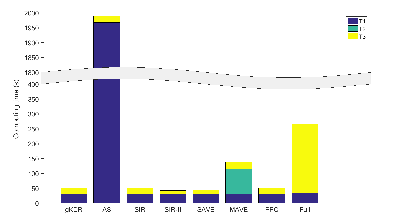
where f^isubscript^๐‘“๐‘–\hat{f}_{i} is the prediction (predictive mean) using emulation. The associated computing time is also recorded with three parts: T1 for running the simulator, T2 for estimating the dimension reduction and T3 for training the emulator and making prediction. Note that T1 includes the time devoted to run the simulator M๐‘€M times when using all the dimension reduction methods. It also includes the time used to compute the gradients for AS and the additional 10โ€‹d10๐‘‘10d runs for full emulation. T2 is zero for full emulation since there is no dimension reduction. T3 also includes the time for running the simulator 10โ€‹d10๐‘‘10d times on the designed points except full emulation.

In this study, we choose M=300๐‘€300M=300 and d=1,โ€ฆ,5๐‘‘1โ€ฆ5d=1,...,5. Tableย 1 presents the results on a testing set with n=500๐‘›500n=500 evaluations using different emulation approaches and Fig.ย 1 shows an example of the associated computing time when ฮฒ=1๐›ฝ1\beta=1 and d=5๐‘‘5d=5. Compared with the full emulation results, by reducing the dimension properly, the predictive accuracy can be improved, especially when the correlation length is long (ฮฒ=1๐›ฝ1\beta=1). Also, as a result, the computing time for training GP emulator (T3) decreases dramatically. In terms of predictive accuracy, AS naturally performs the best, as it is using exact gradients, followed by gKDR. MAVE, SIR and PFC are better than SIR-II and SAVE, but PFC does not work very well when ฮฒ=1๐›ฝ1\beta=1 and MAVE spends more computing time on dimension reduction. Most methods yield smaller errors for ฮฒ=1๐›ฝ1\beta=1 than ฮฒ=0.01๐›ฝ0.01\beta=0.01, except PFC and full emulation. Unlike the other techniques, AS employs exact gradients which explains its lead in performance. However, as shown in Fig.ย 1, the computing time T1 for AS is about two orders of magnitude longer than the others making the method most computationally expensive. Moreover, computing gradients โˆ‡๐ฑfsubscriptโˆ‡๐ฑ๐‘“\nabla_{\mathbf{x}}f is sometimes impossible, e.g. for the tsunami simulation in the next study. This restricts the applicability of AS method to a few applications. To summarize, when the exact gradients are computable the proposed gKDR approach is able to produce comparable results (though not as good) as the AS method that uses exact gradients, and outperforms the other SDR methods in most cases. However, the computational cost of applying gKDR is much less than that employing AS. In fact, gKDR not only is able to find the SDR accurately and efficiently, but also can be applied in a wide range of scenarios where complicated variable types or very high dimensions are involved. The next application into tsunami simulation provides a snapshot of its wide capability when there are few applicable alternatives.

Table 1: Study 1: Normalized PRMSEs at 500500500 testing sites using emulation on the full input space (Full) or combined with different dimension reduction techniques.
ฮฒ=1๐›ฝ1\beta=1
d gKDR AS SIR SIR-II SAVE MAVE PFC Full
1 0.1160.1160.116 0.1260.1260.126 0.1250.1250.125 0.1530.1530.153 0.1530.1530.153 0.1260.1260.126 0.1520.1520.152 0.0970.0970.097
2 0.0440.0440.044 0.0070.0070.007 0.0250.0250.025 0.1530.1530.153 0.1530.1530.153 0.0200.0200.020 0.1400.1400.140 0.0950.0950.095
3 0.0320.0320.032 0.0110.0110.011 0.0240.0240.024 0.1520.1520.152 0.1520.1520.152 0.0190.0190.019 0.1200.1200.120 0.0950.0950.095
4 0.0240.0240.024 0.0120.0120.012 0.0240.0240.024 0.1500.1500.150 0.1500.1500.150 0.0240.0240.024 0.0800.0800.080 0.0930.0930.093
5 0.0240.0240.024 0.0110.0110.011 0.0260.0260.026 0.1500.1500.150 0.1500.1500.150 0.0830.0830.083 0.0710.0710.071 0.0920.0920.092
ฮฒ=0.01๐›ฝ0.01\beta=0.01
1 0.0370.0370.037 0.0330.0330.033 0.0430.0430.043 0.1690.1690.169 0.1690.1690.169 0.0390.0390.039 0.1610.1610.161 0.0320.0320.032
2 0.0330.0330.033 0.0280.0280.028 0.0390.0390.039 0.1690.1690.169 0.1690.1690.169 0.0380.0380.038 0.1600.1600.160 0.0320.0320.032
3 0.0330.0330.033 0.0290.0290.029 0.0390.0390.039 0.1670.1670.167 0.1670.1670.167 0.0390.0390.039 0.0340.0340.034 0.0320.0320.032
4 0.0330.0330.033 0.0250.0250.025 0.0390.0390.039 0.1670.1670.167 0.1670.1670.167 0.0390.0390.039 0.0330.0330.033 0.0320.0320.032
5 0.0330.0330.033 0.0240.0240.024 0.0380.0380.038 0.1670.1670.167 0.1670.1670.167 0.0370.0370.037 0.0330.0330.033 0.0320.0320.032
Refer to caption
Figure 1: Computing time (in seconds) for the emulation using different approaches when ฮฒ=1๐›ฝ1\beta=1 and d=5๐‘‘5d=5.

5.2 Study 2: tsunami emulation where no gradients available

Here we apply the proposed general framework to investigate the impact of uncertainties in the bathymetry on tsunami modeling, where the bathymetry is included as a high-dimensional input.

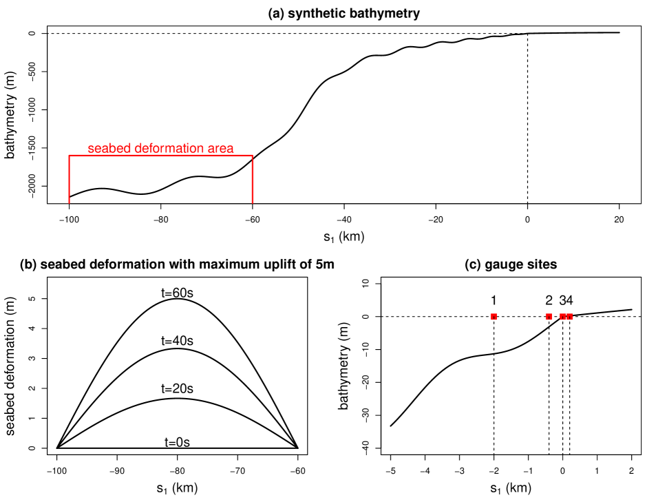
A synthetic bathymetry surface is created in the (s1,s2)subscript๐‘ 1subscript๐‘ 2(s_{1},s_{2}) coordinate system to conduct tsunami simulations as shown in Fig.ย 2 (a). For simplicity, we assume that the seabed elevation only vary along the first coordinate s1subscript๐‘ 1s_{1}. Though simple, it still captures the typical continental characteristics: the continental shelf spans from shore line (s1=0subscript๐‘ 10s_{1}=0) to around s1=โˆ’25subscript๐‘ 125s_{1}=-25 km at the water depth of around 150150150 m; the continental slope is between s1=โˆ’25subscript๐‘ 125s_{1}=-25 km and s1=โˆ’75subscript๐‘ 175s_{1}=-75 km with water depth of 150โˆผ1800similar-to1501800150\sim 1800 m; west of โˆ’7575-75 km it is the deep ocean with water depth of 1800โˆผ2200similar-to180022001800\sim 2200 m .

Refer to caption
Figure 2: (a) Synthetic bathymetry; (b) seabed uplift when hmโ€‹aโ€‹x=5subscriptโ„Ž๐‘š๐‘Ž๐‘ฅ5h_{max}=5 m; (c) gauge sites.

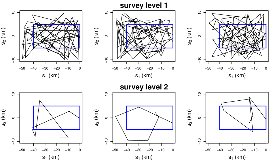
To model uncertainties and mimic the realistic boat tracks of oceanic surveys, some irregular lines are drawn. We consider two levels of survey density which are denoted by survey level 1 and 2 respectively. Considering that the surveys are usually constrained within budgets, the total lengths of the two level surveys are fixed at 100010001000 and 100100100 km. To account for different possible survey traces, 202020 samples of boat tracks are drawn at each level of survey density; see in Fig.ย 3 three samples per level for illustration. In this study, we only consider the impact of the uncertainties in the bathymetry within the area (s1,s2)โˆˆ[โˆ’40000,0]ร—[โˆ’5000,5000]subscript๐‘ 1subscript๐‘ 240000050005000(s_{1},s_{2})\in[-40000,0]\times[-5000,5000] as shown with a blue rectangle in Fig.ย 3. The bathymetry at other locations are fixed at the true values. This assumption is based on the physical knowledge that deep ocean has a relatively small influence on tsunami waves.
Refer to caption
Figure 3: Three samples of boat tracks at two levels of survey density; the bathymetry within the blue rectangle are assumed uncertain.

Along the possible boat tracks, observations of bathymetry are collected every 500500500 m. Then the whole bathymetry surface can be modeled using the SPDE approach [23] and inferred using INLA method[28] for approximate Bayesian inference. Given observations of bathymetry ๐ณ=(z1,โ€ฆ,zn)โ€ฒ๐ณsuperscriptsubscript๐‘ง1โ€ฆsubscript๐‘ง๐‘›โ€ฒ\mathbf{z}=(z_{1},...,z_{n})^{\prime} at locations ๐ฌ=(๐ฌ1,โ€ฆ,๐ฌn)โ€ฒ๐ฌsuperscriptsubscript๐ฌ1โ€ฆsubscript๐ฌ๐‘›โ€ฒ\mathbf{s}=(\mathbf{s}_{1},...,\mathbf{s}_{n})^{\prime}, it is assumed that zi=Zโ€‹(๐ฌi)+ฯตisubscript๐‘ง๐‘–๐‘subscript๐ฌ๐‘–subscriptitalic-ฯต๐‘–z_{i}=Z(\mathbf{s}_{i})+\epsilon_{i}, i=1,โ€ฆ,n๐‘–1โ€ฆ๐‘›i=1,...,n, where the unknown bathymetry surface Zโ€‹(๐ฌ)๐‘๐ฌZ(\mathbf{s}) is Gaussian field with Matรฉrn covariance function

Covโก(Zโ€‹(๐ฌ),Zโ€‹(๐ฌโˆ—))=ฯƒ22ฮฝโˆ’1โ€‹ฮ“โ€‹(ฮฝ)โ€‹(ฮบโ€‹โ€–๐ฌโˆ’๐ฌโˆ—โ€–)ฮฝโ€‹Kฮฝโ€‹(ฮบโ€‹โ€–๐ฌโˆ’๐ฌโˆ—โ€–),Cov๐‘๐ฌ๐‘superscript๐ฌsuperscript๐œŽ2superscript2๐œˆ1ฮ“๐œˆsuperscript๐œ…norm๐ฌsuperscript๐ฌ๐œˆsubscript๐พ๐œˆ๐œ…norm๐ฌsuperscript๐ฌ\operatorname{Cov}(Z(\mathbf{s}),Z(\mathbf{s}^{*}))=\frac{\sigma^{2}}{2^{\nu-1}\Gamma(\nu)}(\kappa\|\mathbf{s}-\mathbf{s}^{*}\|)^{\nu}K_{\nu}(\kappa\|\mathbf{s}-\mathbf{s}^{*}\|), (40)

where โ€–๐ฌโˆ’๐ฌโˆ—โ€–norm๐ฌsuperscript๐ฌ\|\mathbf{s}-\mathbf{s}^{*}\| is the Euclidean distance between two locations ๐ฌ๐ฌ\mathbf{s} and ๐ฌโˆ—โˆˆโ„2superscript๐ฌsuperscriptโ„2\mathbf{s}^{*}\in\mathbb{R}^{2}, Kฮฝsubscript๐พ๐œˆK_{\nu} is the modified Bessel function of the second kind and order ฮฝ>0๐œˆ0\nu>0, ฮบ>0๐œ…0\kappa>0 controls the nominal correlation range through ฯ=8โ€‹ฮฝ/ฮบ๐œŒ8๐œˆ๐œ…\rho=\sqrt{8\nu}/\kappa corresponding to correlations near 0.10.10.1 at the Euclidean distance ฯ๐œŒ\rho, and ฯƒ2superscript๐œŽ2\sigma^{2} is the marginal variance. Lindgren et al. [23] noted that Zโ€‹(๐ฌ)๐‘๐ฌZ(\mathbf{s}) also satisfies the stochastic partial differential equation (SPDE)

ฯ„โ€‹(ฮบ2โˆ’ฮ”)ฮฑ/2โ€‹Zโ€‹(๐ฌ)=Wโ€‹(s),๐œsuperscriptsuperscript๐œ…2ฮ”๐›ผ2๐‘๐ฌ๐‘Š๐‘ \tau(\kappa^{2}-\Delta)^{\alpha/2}Z(\mathbf{s})=W(s), (41)

where the innovation process W๐‘ŠW is spatial Gaussian white noise with unit variance, ฮ”=โˆ‚2โˆ‚s12+โˆ‚2โˆ‚s22ฮ”superscript2superscriptsubscript๐‘ 12superscript2superscriptsubscript๐‘ 22\Delta=\frac{\partial^{2}}{\partial s_{1}^{2}}+\frac{\partial^{2}}{\partial s_{2}^{2}} is the Laplacian operator, and ฯ„๐œ\tau controls the marginal variance through the relationship

ฯ„2=ฮ“โ€‹(ฮฝ)ฮ“โ€‹(ฮฝ+1)โ€‹(4โ€‹ฯ€)โ€‹ฮบ2โ€‹ฮฝโ€‹ฯƒ2.superscript๐œ2ฮ“๐œˆฮ“๐œˆ14๐œ‹superscript๐œ…2๐œˆsuperscript๐œŽ2\tau^{2}=\frac{\Gamma(\nu)}{\Gamma(\nu+1)(4\pi)\kappa^{2\nu}\sigma^{2}}. (42)

With a finite elements representation

Zโ€‹(๐ฌ)=โˆ‘k=1mwkโ€‹ฯˆkโ€‹(๐ฌ),๐‘๐ฌsuperscriptsubscript๐‘˜1๐‘šsubscript๐‘ค๐‘˜subscript๐œ“๐‘˜๐ฌZ(\mathbf{s})=\sum_{k=1}^{m}w_{k}\psi_{k}(\mathbf{s}), (43)

over an appropriate triangular mesh, a stochastic weak solution to the SPDE can be approximated. It is shown that the coefficients ๐ฐ=(w1,โ€ฆ,wm)T๐ฐsuperscriptsubscript๐‘ค1โ€ฆsubscript๐‘ค๐‘š๐‘‡\mathbf{w}=(w_{1},...,w_{m})^{T} can be approximated by a Gaussian Markov random field, i.e. ๐ฐโˆผNโก(๐ŸŽ,๐โˆ’1)similar-to๐ฐN0superscript๐1\mathbf{w}\sim\operatorname{N}(\mathbf{0},\mathbf{Q}^{-1}) for ๐๐\mathbf{Q} is sparse. Note that bivariate splines could be used [24] to reduce the number of parameters required for specific approximation order, which is good, but not enough, for dimension reduction. Then we build the following hierarchical spatial model,

๐ณ|๐ฐ,๐œฝโˆผNโก(๐€๐ฐ,ฯƒe2โ€‹๐ˆ),๐ฐ|๐œฝโˆผNโก(๐ŸŽ,๐โ€‹(๐œฝ)โˆ’1),๐œฝโˆผฯ€โ€‹(๐œฝ),formulae-sequencesimilar-toconditional๐ณ๐ฐ๐œฝN๐€๐ฐsuperscriptsubscript๐œŽ๐‘’2๐ˆformulae-sequencesimilar-toconditional๐ฐ๐œฝN0๐superscript๐œฝ1similar-to๐œฝ๐œ‹๐œฝ\displaystyle\begin{split}\mathbf{z}|\mathbf{w},\boldsymbol{\theta}&\sim\operatorname{N}(\mathbf{Aw},\sigma_{e}^{2}\mathbf{I}),\\ \mathbf{w}|\boldsymbol{\theta}&\sim\operatorname{N}(\mathbf{0},\mathbf{Q}(\boldsymbol{\theta})^{-1}),\\ \boldsymbol{\theta}&\sim\pi(\boldsymbol{\theta}),\end{split}

where ๐€iโ€‹j=ฯˆjโ€‹(๐ฌi)subscript๐€๐‘–๐‘—subscript๐œ“๐‘—subscript๐ฌ๐‘–\mathbf{A}_{ij}=\psi_{j}(\mathbf{s}_{i}) and ๐œฝ๐œฝ\boldsymbol{\theta} contains all the hyperparameters. Since ๐ฐ๐ฐ\mathbf{w} uniquely determines the bathymetry, it is the de facto input for uncertain bathymetry. In this study, we build a mesh for the finite elements representation in the SPDE approach as shown in Fig.ย 4 (a). The dense triangles in the middle cover the uncertain bathymetry area and the outer extension with coarse triangles is added to avoid boundary effect. There are 320032003200 nodes that influence the bathymetry, hence the uncertain input for bathymetry is of dimension 320032003200. Given each boat track and the associated observations ๐ณ๐ณ\mathbf{z}, 202020 samples of the finite element coefficients are drawn from the posterior ฯ€โ€‹(๐ฐ|๐ณ)๐œ‹conditional๐ฐ๐ณ\pi(\mathbf{w}|\mathbf{z}) to construct a range of possible initial bathymetries. Thus there are 400400400 (202020 samples of boat tracks times 202020 samples of ๐ฐ๐ฐ\mathbf{w}) sets of possible initial bathymetries in total at each survey level. Figureย 5 shows the empirical sample mean and standard deviation of these 400400400 possible bathymetries at survey 1 and 2.
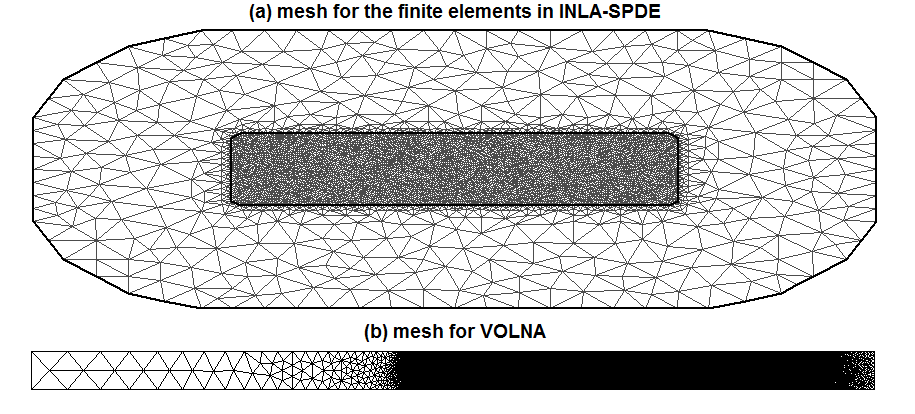
Refer to caption
Figure 4: (a) mesh for SPDE approach; (b) mesh for VOLNA.
Refer to caption
Figure 5: Empirical mean and standard deviation of the 400400400 sets of bathymetry input across both uncertain boat tracks and posterior samples of ๐ฐ๐ฐ\mathbf{w}; note the different scales of standard deviation for survey level 1 and 2.

Tsunami waves are triggered by the following simplified seabed deformation,

dโ€‹zโ€‹(s1,s2;t)=t60โ‹…hmโ€‹aโ€‹xโ‹…sinโก(s1+100000โˆ’60000+100000โ€‹ฯ€)โ‹…I{โˆ’100000โ‰คs1โ‰คโˆ’60000,0โ‰คtโ‰ค60},๐‘‘๐‘งsubscript๐‘ 1subscript๐‘ 2๐‘กโ‹…๐‘ก60subscriptโ„Ž๐‘š๐‘Ž๐‘ฅsubscript๐‘ 110000060000100000๐œ‹subscript๐ผformulae-sequence100000subscript๐‘ 1600000๐‘ก60dz(s_{1},s_{2};t)=\frac{t}{60}\cdot h_{max}\cdot\sin\left(\frac{s_{1}+100000}{-60000+100000}\pi\right)\cdot I_{\{-100000\leq s_{1}\leq-60000,0\leq t\leq 60\}}, (44)

where dโ€‹zโ€‹(s1,s2;t)๐‘‘๐‘งsubscript๐‘ 1subscript๐‘ 2๐‘กdz(s_{1},s_{2};t) is the seabed uplift at location ๐ฌ=(s1,s2)๐ฌsubscript๐‘ 1subscript๐‘ 2\mathbf{s}=(s_{1},s_{2}) and time t๐‘กt, hmโ€‹aโ€‹xsubscriptโ„Ž๐‘š๐‘Ž๐‘ฅh_{max} denotes the maximum seabed uplift; see Fig.ย 2 (b) for example. We take 555 different values hmโ€‹aโ€‹x=1,โ€ฆ,5subscriptโ„Ž๐‘š๐‘Ž๐‘ฅ1โ€ฆ5h_{max}=1,...,5 m. These values are evenly combined with the uncertain initial bathymetry. Thus there are two sources of uncertainties: ๐ฐ๐ฐ\mathbf{w} for bathymetry and hmโ€‹aโ€‹xsubscriptโ„Ž๐‘š๐‘Ž๐‘ฅh_{max} for tsunami source, where ๐ฐ๐ฐ\mathbf{w} is high-dimensional.

We employ the tsunami code VOLNA [12], an advanced non-linear shallow water equation solver using the finite volume method on a high performance computing facility. The computational domain and mesh for VOLNA are presented in Fig.ย 4 (b). There are 120,661120661120,661 triangles and 61,0686106861,068 nodes in the mesh, where the coarse triangles in both ends are added to avoid boundary reflection. The output of the simulation is chosen to be ฮ”โ€‹ฮทโ€‹(๐ฌ)=maxโกฮทtโ€‹(๐ฌ)โˆ’ฮท0โ€‹(๐ฌ)ฮ”๐œ‚๐ฌsubscript๐œ‚๐‘ก๐ฌsubscript๐œ‚0๐ฌ\Delta\eta(\mathbf{s})=\max\eta_{t}(\mathbf{s})-\eta_{0}(\mathbf{s}), where ฮทtโ€‹(๐ฌ)subscript๐œ‚๐‘ก๐ฌ\eta_{t}(\mathbf{s}) is the free surface elevation at simulation time t๐‘กt and location ๐ฌ๐ฌ\mathbf{s}. ฮ”โ€‹ฮทฮ”๐œ‚\Delta\eta represents the maximum wave height at off shore locations or the maximum inundation depth at on shore locations. For illustration, we consider simulation values at gauge 1: (โˆ’2000,0)20000(-2000,0), gauge 2: (โˆ’400,0)4000(-400,0), gauge 3: (0,0)00(0,0) and gauge 4: (200,0)2000(200,0), which are at far shore, near shore, shore line and land respectively; see Fig.ย 2 (c).

The simulation results are presented in Fig.ย 6, with those using the true bathymetry shown in red lines and those using the sample mean bathymetry shown in green dash lines. We can see that ฮ”โ€‹ฮทฮ”๐œ‚\Delta\eta increases with hmโ€‹aโ€‹xsubscriptโ„Ž๐‘š๐‘Ž๐‘ฅh_{max} but also shows variation due to the uncertain inputs ๐ฐ๐ฐ\mathbf{w} for fixed hmโ€‹aโ€‹xsubscriptโ„Ž๐‘š๐‘Ž๐‘ฅh_{max}, especially at gauges 2-4 around the shore line. In general, the simulations with sample mean bathymetry would deviate from true values, while those with random bathymetry samples can cover the true events quite well. The survey level also has significant influence that differs across the four gauges. In most cases the wider range of possible simulation values with coarser survey level 2 indicates that the uncertainty in the bathymetry would spread the tsunami waves out to simulate more extreme scenarios and such effect could be amplified around the shore line.
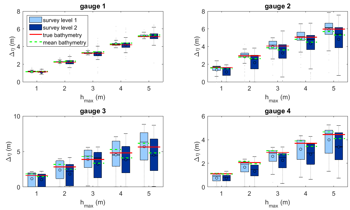
Refer to caption
Figure 6: Simulation values with different inputs (๐ฐ,hmโ€‹aโ€‹x)๐ฐsubscriptโ„Ž๐‘š๐‘Ž๐‘ฅ(\mathbf{w},h_{max}) at four gauges. The uncertain input ๐ฐ๐ฐ\mathbf{w} are drawn based on survey level 1 and 2, together with the true values and sample mean values.

Following the procedure in Sectionย 4, we can construct a low-dimensional emulator for such high dimensional simulator with 320032003200 input parameters for the bathymetry (๐ฐ๐ฐ\mathbf{w}) and 111 parameter for the seabed deformation (hmโ€‹aโ€‹xsubscriptโ„Ž๐‘š๐‘Ž๐‘ฅh_{max}). Denoting the VOLNA code with f๐‘“f, the output can be represented as ฮ”โ€‹ฮท=fโ€‹(๐ฐ,hmโ€‹aโ€‹x).ฮ”๐œ‚๐‘“๐ฐsubscriptโ„Ž๐‘š๐‘Ž๐‘ฅ\Delta\eta=f(\mathbf{w},h_{max}). Because Fig.ย 6 displays a significant relationship between hmโ€‹aโ€‹xsubscriptโ„Ž๐‘š๐‘Ž๐‘ฅh_{max} and ฮ”โ€‹ฮทฮ”๐œ‚\Delta\eta, we keep it as a separate input in the emulator and reduce the dimension of ๐ฐ๐ฐ\mathbf{w} only. In this case, we try to find a projection matrix ๐๐\mathbf{B} such that ๐ฐโŸ‚(ฮ”โ€‹ฮท,hmโ€‹aโ€‹x)|๐Tโ€‹๐ฐperpendicular-to๐ฐconditionalฮ”๐œ‚subscriptโ„Ž๐‘š๐‘Ž๐‘ฅsuperscript๐๐‘‡๐ฐ\mathbf{w}\perp(\Delta\eta,h_{max})|\mathbf{B}^{T}\mathbf{w}. The conditional independence just implies the sufficiency of ๐Tโ€‹๐ฐsuperscript๐๐‘‡๐ฐ\mathbf{B}^{T}\mathbf{w}, i.e. pโ€‹(ฮ”โ€‹ฮท|hmโ€‹aโ€‹x,๐ฐ)=p~โ€‹(ฮ”โ€‹ฮท|hmโ€‹aโ€‹x,๐Tโ€‹๐ฐ)๐‘conditionalฮ”๐œ‚subscriptโ„Ž๐‘š๐‘Ž๐‘ฅ๐ฐ~๐‘conditionalฮ”๐œ‚subscriptโ„Ž๐‘š๐‘Ž๐‘ฅsuperscript๐๐‘‡๐ฐp(\Delta\eta|h_{max},\mathbf{w})=\tilde{p}(\Delta\eta|h_{max},\mathbf{B}^{T}\mathbf{w}) [31]. Therefore, (ฮ”โ€‹ฮท,hmโ€‹aโ€‹x)ฮ”๐œ‚subscriptโ„Ž๐‘š๐‘Ž๐‘ฅ(\Delta\eta,h_{max}) is regarded as a temporary output when applying gKDR to reduce the dimension of ๐ฐ๐ฐ\mathbf{w}.

For the gKDR approach, Gaussian RBF kernels kโ€‹(x,y)=expโก(โ€–xโˆ’yโ€–2/(2โ€‹ฯƒ2))๐‘˜๐‘ฅ๐‘ฆsuperscriptnorm๐‘ฅ๐‘ฆ22superscript๐œŽ2k(x,y)=\exp(\|x-y\|^{2}/(2\sigma^{2})) are deployed for both k๐’ณsubscript๐‘˜๐’ณk_{\mathcal{X}} and k๐’ดsubscript๐‘˜๐’ดk_{\mathcal{Y}} but with different parameters ฯƒ2superscript๐œŽ2\sigma^{2}. Following [15], we have the parameterization ฯƒ๐’ณ=c1โ€‹ฯƒmโ€‹eโ€‹dโ€‹(๐—)subscript๐œŽ๐’ณsubscript๐‘1subscript๐œŽ๐‘š๐‘’๐‘‘๐—\sigma_{\mathcal{X}}=c_{1}\sigma_{med}(\mathbf{X}), ฯƒY=c2โ€‹ฯƒmโ€‹eโ€‹dโ€‹(๐˜)subscript๐œŽ๐‘Œsubscript๐‘2subscript๐œŽ๐‘š๐‘’๐‘‘๐˜\sigma_{Y}=c_{2}\sigma_{med}(\mathbf{Y}) where ฯƒmโ€‹eโ€‹dโ€‹(โ‹…)subscript๐œŽ๐‘š๐‘’๐‘‘โ‹…\sigma_{med}(\cdot) is the median of pairwise distance of the data. The regularization parameter ฯตnsubscriptitalic-ฯต๐‘›\epsilon_{n} is fixed at 10โˆ’5superscript10510^{-5} because its influence is shown to be negligible after a few trials. There are three parameters to be specified properly: c1subscript๐‘1c_{1}, c2subscript๐‘2c_{2}, and d๐‘‘d, the number of directions included in the emulator. We consider possible candidates c1,c2โˆˆ[0.5,1,5,10,15,20]subscript๐‘1subscript๐‘20.515101520c_{1},c_{2}\in[0.5,1,5,10,15,20], dโˆˆ[1,โ€ฆ,5]๐‘‘1โ€ฆ5d\in[1,...,5] here. Then, based on each of the possible parameters combination, we can construct a GP emulator on the low-dimensional inputs (hmโ€‹aโ€‹x,๐Tโ€‹๐ฐ)subscriptโ„Ž๐‘š๐‘Ž๐‘ฅsuperscript๐๐‘‡๐ฐ(h_{max},\mathbf{B}^{T}\mathbf{w}) and make predictions on the new inputs (h~mโ€‹aโ€‹x,๐Tโ€‹๐ฐ~)subscript~โ„Ž๐‘š๐‘Ž๐‘ฅsuperscript๐๐‘‡~๐ฐ(\tilde{h}_{max},\mathbf{B}^{T}\tilde{\mathbf{w}}).

For comparison, we also apply alternative dimension reduction techniques to construct the low-dimensional approximations. Due to the complexity of the VOLNA code, the gradients of simulation values with respect to the inputs are not computable. Hence the active subspace method cannot be employed. Most of the methods in Study 1 cannot be applied directly because of the need for partial dimension reduction, or the โ€œlarge p๐‘p, small n๐‘›nโ€ feature, i.e. there are much more input parameters than the number of simulations. We consider two extensions to PFC and SIR. The partial PFC (PPFC) method [20] is implemented based on the R package ldr [1] to find the reduction on ๐ฐ๐ฐ\mathbf{w} only meanwhile taking the effect of hmโ€‹aโ€‹xsubscriptโ„Ž๐‘š๐‘Ž๐‘ฅh_{max} into account. Note that PFC is not developed for the problem where p>n๐‘๐‘›p>n or pโ‰ซnmuch-greater-than๐‘๐‘›p\gg n. Another method we compare to is the sequential sufficient dimension reduction (SSDR) [31]. It is specifically proposed to overcome the โ€œlarge p๐‘p, small n๐‘›nโ€ difficulty by decomposing the variables into pieces each of which has p1<nsubscript๐‘1๐‘›p_{1}<n variables so that conventional dimension reduction methods can be applied. The projective resampling approach [21] with SIR is employed. The R code for SSDR by [31] is available from http://wileyonlinelibrary.com/journal/rss-datasets.

To measure the predictive performance and select proper parameters, a 101010-fold cross validation approach is employed. For each survey level, 400400400 simulations are divided evenly into 101010 groups. Each group is retained as testing set once, while the other nine groups are used to estimate the projection matrix ๐๐\mathbf{B} using the gKDR, PPFC or SSDR approaches and train the respective GP emulator. Tableย 2 presents the normalized PRMSEs from the cross validation for each survey level and gauge using different dimension reduction techniques. The errors of survey level 1 are in general smaller than those of survey level 2. This implies that as the uncertainties in the bathymetry increase, it gets more difficult to make accurate predictions using emulation. The methods gKDR and SSDR outperform PPFC in all cases, especially in survey level 1 where the normalized PRMSEs can be 50%percent5050\% lower in some cases. In survey level 1, the errors of the gKDR approach are slightly larger than those of the SSDR for gauge 2-4 where the normalized PRMSEs using SSDR are around 1.1%โˆผ3.7%similar-topercent1.1percent3.71.1\%\sim 3.7\% lower. But in survey level 2, the gKDR approach is more accurate than the SSDR approach for all gauges with reduction of normalized PRMSEs at 1.0%percent1.01.0\% for gauge 1 and 10.1%โˆผ18.9%similar-topercent10.1percent18.910.1\%\sim 18.9\% for gauge 2-4. Therefore, gKDR is comparable with SSDR in survey level 1 but works much better than SSDR in survey level 2 when there are more uncertainties involved. We can conclude that the proposed GP emulation framework combined with the gKDR dimension reduction approach is effective and accurate for this complicated tsunami simulator and overall it outperforms the alternatives.

Table 2: Study 2: Normalized PRMSEs of the 10-fold cross validation using GP emulation combined with different dimension reduction methods.
gauge survey level 1 survey level 2
gKDR PPFC SSDR gKDR PPFC SSDR
1 0.0310.0310.031 0.0780.0780.078 0.0330.0330.033 0.0950.0950.095 0.0960.0960.096 0.0960.0960.096
2 0.0990.0990.099 0.1380.1380.138 0.0970.0970.097 0.1340.1340.134 0.1750.1750.175 0.1490.1490.149
3 0.0910.0910.091 0.1870.1870.187 0.0900.0900.090 0.1290.1290.129 0.2100.2100.210 0.1590.1590.159
4 0.0820.0820.082 0.1440.1440.144 0.0790.0790.079 0.1060.1060.106 0.1410.1410.141 0.1210.1210.121

To investigate the impact of the training set size on the predictive performance of the proposed emulation framework with gKDR, we conduct repeated random sub-sampling cross validations with various training set sizes. We consider training set size as 2%percent22\%, 5%percent55\%, 10%percent1010\%, 20%percent2020\%, โ€ฆ, 90%percent9090\% and test set size as 10%percent1010\% of the total 400400400 simulations. For each training set size, the sampling is repeated 505050 times. The parameters c1,c2,dsubscript๐‘1subscript๐‘2๐‘‘c_{1},c_{2},d are fixed at those values selected through the above 10-fold cross validation. Figureย 7 displays the normalized PRMSEs with various training set sizes. In general, the predictive errors decrease as the training set size increases, and eventually converge to a relatively flat level, after about 100100100 simulations. It is reassuring that such a small number of simulations is enough to allow an efficient and effective dimension reduction and Gaussian process emulation.
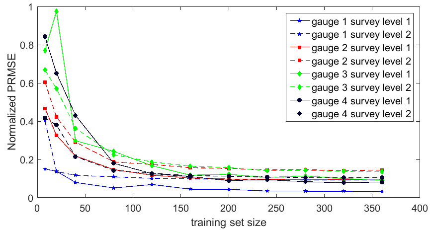
Refer to caption
Figure 7: Normalized PRMSEs with various training set sizes.

In the end, we apply the resulting emulator to predict the simulation values over a large number of new inputs. The predictions can be used for probabilistic risk assessment and many other purposes. For illustration, 10,0001000010,000 samples of (h~mโ€‹aโ€‹x,๐ฐ~)subscript~โ„Ž๐‘š๐‘Ž๐‘ฅ~๐ฐ(\tilde{h}_{max},\tilde{\mathbf{w}}) are drawn where h~mโ€‹aโ€‹xsubscript~โ„Ž๐‘š๐‘Ž๐‘ฅ\tilde{h}_{max} are drawn from a Normal distribution Nโก(3,1)N31\operatorname{N}(3,1) truncated at 00 and 555. For each survey level, 100100100 samples of possible boat tracks are drawn randomly. Given the observations along each boat track, 100100100 samples of ๐ฐ~~๐ฐ\tilde{\mathbf{w}} are drawn from the posterior. In most of the current tsunami research work, the bathymetry is usually considered as fixed, which would neglect the possible uncertainty in the outputs. For comparison, we also conduct another set of simulations with the 555 possible values of hmโ€‹aโ€‹xsubscriptโ„Ž๐‘š๐‘Ž๐‘ฅh_{max}, but with a fixed ๐ฐ๐ฐ\mathbf{w} taken to be the sample mean shown in Fig.ย 5. In this case, hmโ€‹aโ€‹xsubscriptโ„Ž๐‘š๐‘Ž๐‘ฅh_{max} is the only uncertain parameter. Then we can also make another set of predictions on the 10,0001000010,000 samples of h~mโ€‹aโ€‹xsubscript~โ„Ž๐‘š๐‘Ž๐‘ฅ\tilde{h}_{max} only. The predictions for these two cases are presented in Fig.ย 8. We can see that at gauge 1 it makes no significant difference to include the uncertainty in the bathymetry or not, as the impact is relatively small on the far shore waves, as shown in Fig.ย 6. However, the impact of the uncertainty in the bathymetry on the simulation values is more significant at gauges around the shore line. The distributions are shifted, skewed and spread out, covering more extreme events with larger ฮ”โ€‹ฮทฮ”๐œ‚\Delta\eta. These features are potentially important, for example in the catastrophe models for (re)insurance, or hazard assessment used in coastal planning.
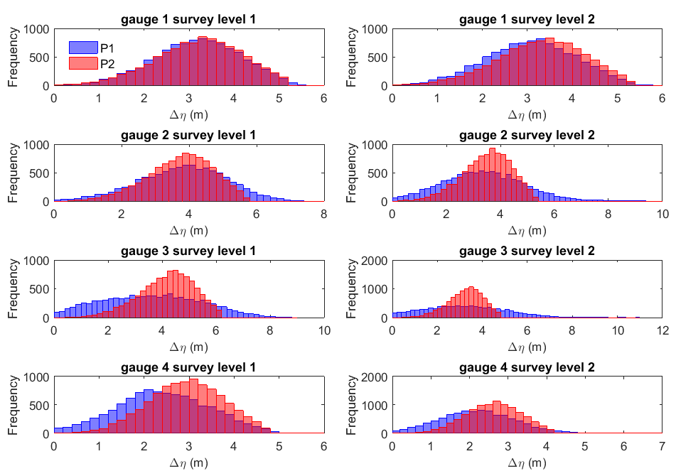
Refer to caption
Figure 8: Histogram of predictions of 10,0001000010,000 tsunami wave heights at four gauges due to the uncertain seabed uplift (prediction P2). Prediction P1 also accounts for the uncertainties in the bathymetry. Left column: high-resolution bathymetry survey (level 1); Right column: coarse bathymetry survey (level 2).

6 Discussion

We proposed a joint framework for emulation of high-dimensional simulators with dimension reduction. The gKDR approach is employed to construct low-dimensional approximations to the simulators. The approximations retain most of the information about the input-output behavior and make the emulation much more efficient. Both theoretical properties and numerical studies have demonstrated the efficiency and accuracy of the proposed approach and its advantages over other dimension reduction techniques. Our method can be applied for many purposes of uncertainty quantification such as risk assessment, sensitivity analysis and calibration, with great perspectives in real world applications.

There are some practical issues when applying the proposed framework. The hyperparameters in gKDR and the number of dimensions to be included in the emulator need to be specified properly. In practice, a simple trial and error procedure could be applied, especially when the results are not very sensitive to the choices. Cross validation steps could also benefit from parallel computing technique. The sample size also affect the predictive ability of the final emulator, as sufficient samples are needed to estimate the dimension reduction accurately. A diagnostic plot of predictive errors with increasing number of sizes such as Fig.ย 7 could help identify the convergence. After determining the dimension reduction, a sufficient number of training samples with a proper design are often required to train the emulator in order to balance the computational cost and accuracy. The benefits of our approach are multiple. One can tackle uncertainty quantification tasks for complex models where boundary conditions are of high dimension. Beyond tsunami modeling, in climate simulation, weather forecasting or geophysical sciences, uncertainty quantification studies would become tractable and potentially offer solutions to important scientific problems.

References

  • [1] K.ย P. Adragni and A.ย Raim, ldr: an R software package for likelihood-based sufficient dimension reduction, Journal of Statistical Software, 61 (2014), pp.ย 1โ€“21.
  • [2] A.ย A. Amini and M.ย J. Wainwright, Sampled forms of functional PCA in reproducing kernel Hilbert spaces, The Annals of Statistics, 40 (2012), pp.ย 2483โ€“2510.
  • [3] I.ย Andrianakis and P.ย G. Challenor, The effect of the nugget on Gaussian process emulators of computer models, Computational Statistics & Data Analysis, 56 (2012), pp.ย 4215โ€“4228.
  • [4] J.ย Beck and S.ย Guillas, Sequential design with mutual information for computer experiments (MICE): emulation of a tsunami model, SIAM/ASA Journal on Uncertainty Quantification, 4 (2016), pp.ย 739โ€“766.
  • [5] P.ย Constantine and D.ย Gleich, Computing active subspaces with Monte Carlo, July 2015.
  • [6] P.ย G. Constantine, E.ย Dow, and Q.ย Wang, Active subspace methods in theory and practice: applications to kriging surfaces, SIAM Journal on Scientific Computing, 36 (2014), pp.ย A1500โ€“A1524.
  • [7] R.ย D. Cook, On the interpretation of regression plots, Journal of the American Statistical Association, 89 (1994), pp.ย 177โ€“189.
  • [8] ย , Fisher lecture: dimension reduction in regression, Statistical Science, (2007), pp.ย 1โ€“26.
  • [9] ย , Regression graphics: ideas for studying regressions through graphics, vol.ย 482, John Wiley & Sons, 2009.
  • [10] R.ย D. Cook and L.ย Forzani, Principal fitted components for dimension reduction in regression, Statistical Science, 23 (2008), pp.ย 485โ€“501.
  • [11] R.ย D. Cook and S.ย Weisberg, Discussion of โ€œsliced inverse regression for dimension reductionโ€ by li, k.c., Journal of the American Statistical Association, 86 (1991), pp.ย 328โ€“332.
  • [12] D.ย Dutykh, R.ย Poncet, and F.ย Dias, The VOLNA code for the numerical modeling of tsunami waves: generation, propagation and inundation, European Journal of Mechanics-B/Fluids, 30 (2011), pp.ย 598โ€“615.
  • [13] G.ย E. Fasshauer, Positive definite kernels: past, present and future, Dolomite Research Notes on Approximation, 4 (2011), pp.ย 21โ€“63.
  • [14] K.ย Fukumizu, F.ย R. Bach, and M.ย I. Jordan, Dimensionality reduction for supervised learning with reproducing kernel Hilbert spaces, The Journal of Machine Learning Research, 5 (2004), pp.ย 73โ€“99.
  • [15] K.ย Fukumizu and C.ย Leng, Gradient-based kernel dimension reduction for regression, Journal of the American Statistical Association, 109 (2014), pp.ย 359โ€“370.
  • [16] G.ย H. Golub and C.ย F. Vanย Loan, Matrix computations, vol.ย 3, JHU Press, 2012.
  • [17] A.ย Gretton, K.ย M. Borgwardt, M.ย J. Rasch, B.ย Schรถlkopf, and A.ย Smola, A kernel two-sample test, The Journal of Machine Learning Research, 13 (2012), pp.ย 723โ€“773.
  • [18] D.ย A. Henderson, R.ย J. Boys, K.ย J. Krishnan, C.ย Lawless, and D.ย J. Wilkinson, Bayesian emulation and calibration of a stochastic computer model of mitochondrial DNA deletions in substantia nigra neurons, Journal of the American Statistical Association, 104 (2009), pp.ย 76โ€“87.
  • [19] B.ย Iooss and M.ย Ribatet, Global sensitivity analysis of computer models with functional inputs, Reliability Engineering & System Safety, 94 (2009), pp.ย 1194โ€“1204.
  • [20] D.ย H. Kim, Partial Sufficient Dimension Reduction in Regression, PhD thesis, University of Minnesota, 2011.
  • [21] B.ย Li, S.ย Wen, and L.ย Zhu, On a projective resampling method for dimension reduction with multivariate responses, Journal of the American Statistical Association, 103 (2008), pp.ย 1177โ€“1186.
  • [22] K.-C. Li, Sliced inverse regression for dimension reduction (with discussion), Journal of the American Statistical Association, 86 (1991), pp.ย 316โ€“327.
  • [23] F.ย Lindgren, H.ย Rue, and J.ย Lindstrรถm, An explicit link between Gaussian fields and Gaussian Markov random fields: the stochastic partial differential equation approach, Journal of the Royal Statistical Society: Series B (Statistical Methodology), 73 (2011), pp.ย 423โ€“498.
  • [24] X.ย Liu, S.ย Guillas, and M.-J. Lai, Efficient spatial modelling using the SPDE approach with bivariate splines, Journal of Computational and Graphical Statistics, accepted (2015).
  • [25] A.ย Marrel, B.ย Iooss, S.ย Daย Veiga, and M.ย Ribatet, Global sensitivity analysis of stochastic computer models with joint metamodels, Statistics and Computing, 22 (2012), pp.ย 833โ€“847.
  • [26] A.ย Oโ€™Hagan, Kendallโ€™s advanced theory of statistics, Volume 2B: Bayesian inferenc, Edward Arnold, London, 1994.
  • [27] C.ย E. Rasmussen and C.ย K.ย I. Williams, Gaussian processes for machine learning, The MIT Press, 2006.
  • [28] H.ย Rue, S.ย Martino, and N.ย Chopin, Approximate Bayesian inference for latent Gaussian models by using integrated nested Laplace approximations, Journal of the Royal Statistical Society: Series B (Statistical Methodology), 71 (2009), pp.ย 319โ€“392.
  • [29] J.ย Sacks, W.ย J. Welch, T.ย J. Mitchell, and H.ย P. Wynn, Design and analysis of computer experiments, Statistical science, (1989), pp.ย 409โ€“423.
  • [30] Y.ย Xia, H.ย Tong, W.ย Li, and L.-X. Zhu, An adaptive estimation of dimension reduction space, Journal of the Royal Statistical Society: Series B (Statistical Methodology), 64 (2002), pp.ย 363โ€“410.
  • [31] X.ย Yin and H.ย Hilafu, Sequential sufficient dimension reduction for large p๐‘p, small n๐‘›n problems, Journal of the Royal Statistical Society: Series B (Statistical Methodology), 77 (2015), pp.ย 879โ€“892.