Approximate Personalized PageRank on Dynamic Graphs
Hongyang Zhang
Department of Computer Science
Stanford University
hongyang@cs.stanford.eduPeter Lofgren
Department of Computer Science
Stanford University
plofgren@cs.stanford.eduAshish Goel
Department of Management Science and Engineering
Stanford University
ashishg@stanford.edu
Abstract
We propose and analyze two algorithms for maintaining approximate Personalized PageRank (PPR) vectors on a dynamic graph, where edges are added or deleted. Our algorithms are natural dynamic versions of two known local variations of power iteration. One, Forward Push, propagates probability mass forwards along edges from a source node, while the other, Reverse Push, propagates local changes backwards along edges from a target. In both variations, we maintain an invariant between two vectors, and when an edge is updated, our algorithm first modifies the vectors to restore the invariant, then performs any needed local push operations to restore accuracy.
For Reverse Push, we prove that for an arbitrary directed graph in a random edge model, or for an arbitrary undirected graph, given a uniformly random target node , the cost to maintain a PPR vector to of additive error as edges are updated is , where is the average degree of the graph. This is work per update, plus the cost of computing a reverse vector once on a static graph. For Forward Push, we show that on an arbitrary undirected graph, given a uniformly random start node , the cost to maintain a PPR vector from of degree-normalized error as edges are updated is , which is again per update plus the cost of computing a PPR vector once on a static graph.
1 Introduction
Personalized PageRank (PPR) models the relevance of nodes in a network from the point of view of a given node. It has applications in search [13, 12], friend recommendations [4, 11], community detection [22, 2], video recommendations [6], and other applications. Because PPR is expensive to compute at query time, several authors have proposed pre-computing it for each user and storing it [13, 7, 8]. However, in practice graphs are dynamic, for example on a social network users are constantly adding new edges to the network, so we need a method of updating pre-computed PPR values. In this work, we propose two new algorithms for updating pre-computed PPR vectors and give the first rigorous analysis of their running time.
There are four main algorithms for computing PPR [15], of which only one has an analysis for dynamic graphs prior to our work. The first is power iteration [21], but it is very slow, requiring time per user (where is the number of edges), so it can’t be used efficiently for PPR even on static graphs. The second, Forward Push [7, 2], is a local variation of power iteration which starts from the source user (the node whose point of view we take) and pushes probability mass forwards along edges. Berkin [7] proposed pre-computing Forward Push vectors from many source nodes, and Ohsaka et al. [20] proposed an algorithm for updating it on dynamic graphs, however no past work has analyzed the running time for maintaining Forward Push. The third, Reverse Push [13, 2], is an alternative variation of power iteration which starts at each target node and pushes values backwards along edges to improve estimates. Jeh and Widom [13] and Lofgren et al. [17] propose pre-computing Reverse Push vectors (or a variation on them), to enable efficient search, but no past work has proposed an algorithm for updating Reverse Push vectors on dynamic graphs. Finally, a fourth method of computing PPR is Monte-Carlo [3, 9], and for that algorithm Bahmani et al. [5] give an efficient algorithm for updating it on dynamic graphs, with running time analysis in a random edge arrival order model. In experiments, Ohsaka et al. [20] find that when maintaining very accurate PPR vectors, Monte-Carlo is slower than Forward-Push, motivating the analysis of updating Forward Push.
Our contribution is the first running time guarantees for updating Forward Push on undirected graphs and for updating Reverse Push on directed as well as undireted graphs. The analysis is challenging because a new edge at one node can cause that node to push, which can cause a cascade of other nodes to push. Understanding and bounding the size of this cascade required a novel amortized analysis.
We allow for a worst case graph, but we assume that edge updates arrive in a random order to better capture performance in practice. The same assumption was used in the analysis of Monte Carlo [5] where the bounds it leads to were found to model the running time in practice on Twitter. Alternatively, for undirected graphs we prove a worst-case amortized running time. In addition, for undirected graphs, we strengthen the analysis of Monte-Carlo on dynamic graphs [5] to a worst-case edge arrival order.
Our algorithms are simple to implement, and we present two experiments for forward push. One insight from our theoretical analysis is a different way of updating Forward Push values than the previously proposed method [20], and we find that our variation is 1.5-3.5 times faster than that method without sacrificing accuracy.
In the second experiment, we evaluate forward push for the problem of finding the top K highest personalized PageRank
from a source node.
We compare to the Monte-Carlo method of Bahmani et al. [5] and found that
the forward push is 4.5-12 times more efficient in storage compared to Monte-Carlo,
and is able to do edge update 1.5 - 2.5 times faster.
The main idea of our algorithms is that both Forward Push and Reverse Push maintain an invariant between a pair of vectors, and when an edge is added or deleted, we first restore the invariant with an efficient change to the vectors, then perform local push operations as needed to control the error.
One limitation of our analysis is that it applies to the pure versions of Forward Push and Reverse Push, while some prior work [13, 7] proposes combining Forward or Reverse push vectors together, but we believe our analysis would extend to that case. It would also be interesting to extend our analysis adapt the Personalized PageRank search index of [17] to dynamic graphs.
Results
For the Reverse Push algorithm, we show that on a worst-case graph, for a uniform random target, the expected time required to maintain PPR estimates at accuracy to that target as edge updates arrive in a random order is . Here is the desired additive error of the estimates, and is the average degree of nodes in the graph. Since a random PPR value is , values smaller than are not very meaningful. Hence typically and our running time is . Since is the expected time required to compute Reverse Push from scratch [1, 15], we see that our incremental algorithm can maintain estimates after every edge update using time per update and the time required to compute a single Reverse Push vector.
For the Forward Push algorithm, we show that on an arbitrary undirected graph and arbitrary edge arrival order, for a uniform random source node , the worst-case running time to maintain a PPR vector from that source node is . Here is a bound on the degree-normalized error (which we define later). Typically , so this is . The cost of computing such a PPR vector from scratch is [2] so we again see that the cost to maintain the PPR vector over updates is per update plus the cost of computing it once from scratch.
One observation that follows from our work is that for Monte-Carlo, for an arbitrary undirected graph and arbitrary edge arrival order, the time required to maintain random walks from every source node over arrivals is .
This contrasts with a worst-case example constructed on directed graphs
where the total running time to maintain these walks grows super-linear in [14].
Our observation suggests a weaker yet still meaningful bound without the random edge assumption made in Bahmani et al. [5]
for Monte-Carlo methods on undirected graphs.
2 Preliminaries
Let be an unweighted directed graph.
Let denote the adjacency matrix of and
let denote the diagonal matrix representing the outdegrees of all vertices in .
For a vertex , let denote the set of out neighbors of
and let denote the set of in neighbors of .
The personalized PageRank vector for a source node is defined as the unique solution of the following linear system ([21]):
(1)
where (a.k.a. the teleport probability) is a constant between and ,
and is the indicator vector with a single nonzero entry of at .
For a pair of vertices and on ,
we will use to denote the personalized PageRank from to .
This linear algebraic definition of personalized PageRank is equivalent to simulating a random walk.
Start from the source node ,
with probability , go to a uniformly chosen neighbor of the current node,
or with probability stop at the current node:
is the probability that a random walk from stops at [21].
In the above definitions, we assumed that the outdegree of every vertex is at least one for simplicity.
If a vertex has no out neighbors, then the random walk transitions to with probability
(cf. Gleich [10] for other ways to handle dangling nodes).
2.1 The edge arrival model
In the dynamic edge arrival model, we start with an initial graph and there is a sequence of edge updates one by one.
Let denote the initial graph.
Let denote the number of edge updates.
When the -th edge arrives,
if is already in , then it will be deleted; else it will be added to .
Let denote the updated graph.
Note that can differ from by at most two vertices.
Let denote the outdegree of on and denote its indegree.
Also let denote the diagonal matrix of the outdegrees of .
Let denote the personalized PageRank from to on .
Let denote the number of vertices and denote the number of edges in the initial graph .
We will analyze the following two edge arrival models:
To introduce this graph model in our notation,
consider a uniformly random edge permutation of .
Then is the subgraph consisting of the first edges in the permutation.
And is defined as the -th edge in this permutation,
for .
In a uniformly random edge stream, the personalized PageRank vector does not change by “too much”
after an edge update [5].
This intuition is not true in the worst case —
there exists a sequence of edge insertions such that for a single source node,
the aggregate difference between the personalized
PageRank vector before and after every edge insertion
grows superlinear in the number of of nodes [14].
Arbitrary edge updates of undirected graphs
For undirected graph, we observe a few
interesting properties for personalized PageRank, which will be used later.
The first one exploits the fact that on an undirected graph,
a random walk can be in either direction.
The random walk interpretation of personalized PageRank leads to the following general
class of local computation algorithms:
start with all the probability mass on the source node of the graph,
and iteratively push this mass out to neighboring nodes,
getting progressively better approximations.
In these “local push” algorithms, we typically maintain a “residual” at every node,
which is mass that has been received but not yet been pushed out from that node,
as well as an “estimate”, which is mass that has been both received and pushed out
(after accounting for the teleport probability and the outdegrees), we will now
precisely describe how this local approach can be used in the forward and reverse
direction.
2.2.1 Forward push
Given a source node , the forward push algorithm maintains an estimate of for each target .
It also maintains a residual for .
Let denote the the vector of estimates and
the vector of residuals.
The estimates and residuals satisfy the following
invariant property (cf. Section in Lofgren [2]):
(2)
Algorithm 1 described below is a variant of the classic forward local push algorithm [2],
the difference being that we added negative residuals.
As we will see later on, an edge arrival can result in negative residuals —
the edge update affects the amount of residuals a vertex have pushed out.
During a forward push iteration for vertex (Step 7 in Algorithm 1),
an fraction of ’s residual will be added to ’s estimate.
For the rest of fraction, each out neighbor of receives an equal proportion
of .
Algorithm 1 repeatedly perform forward push iterations,
first for vertices with positive residuals and then for vertices with negative residuals,
until for every vertex, its residual divided by the outdegree is within and .
It’s clear that while we work on vertices with negative residuals,
no vertices whose residual is positive and below will increase above .
Algorithm 1ForwardLocalPush
1:()
2:whiledo
3: FwdPush(u)
4:whiledo
5: FwdPush(u)
6:return ()
7:procedureFwdPush()
8:
9:fordo
10:
11:
2.2.2 Reverse push
Given a target node ,
the reverse push algorithm maintains an estimate of , for every node in .
It also maitains a residual for .
Let denote the vector of estimates and for the vector of residuals.
Similar to forward push, estimates and residuals satisfy an invariant property [1, 18]:
(3)
In Algorithm 2 below, we’ve also added negative residuals.
A reverse push iteration on vertex works backward (step 7):
an fraction of ’s residuals goes to ’s estimate;
to push back the other fraction to an in neighbor of , it takes into account
the outdegree of , hence the amount is the residual amount times .
Algorithm 2 keeps pushing residuals back from each vertex,
until the residual of every vertex is within and .
When this happens, it is guaranteed that (cf. Theorem in Anderson et al. [1]).
Algorithm 2ReverseLocalPush
1:()
2:whiledo
3: RevPush(u)
4:whiledo
5: RevPush(u)
6:return ()
7:procedureRevPush()
8:
9:fordo
10:
11:
2.3 Random walks
A well known method in dynamic settings uses random walks
to maintain the personalized PageRank vector.
The algorithm together with an analysis is first introduced by Bahmani et al. [5].
The observation is that an edge update will only affect walks that visited the vertices of the edge.
As an example, suppose that edge is inserted.
If a random walk visits , it should go through edge with probability
.
Therefore, the random walk can be reroute from by generating a new walk segment from .
We repeat the rerouting procedure for each visit at , unless the random walk has been
rerouted already.
The expected number of random walks that needs to be rerouted is given below.
Let be a directed graph and be a vertex of the graph.
Let be a random walk from .
Now suppose that an edge is inserted to .
Then the probability that needs to be updated is at most .
3 Dynamic local push algorithms
Given a node, we can run push algorithms to initialize its data structures that include the estimates and residuals.
If an edge is inserted/deleted,
we can obtain a new pair of estimates and residuals,
by adjusting them locally at the updated edge using the invariant equations.
Since this adjustment can create residuals that gets above or below ,
we then invoke Algorithm 1 (or Algorithm 2) to push residuals from such nodes.
While the idea is simple, the analysis of the number of push iterations is quite intricate.
For the rest of this section, we describe an approach to obtain dynamic local push algorithms and show
how to analyze their running time.
We will introduce a dynamic reverse push algorithm in the first part.
Then we will introduce a dynamic forward push algorithm in the second part.
Finally we will consider how to extend the algorithms to handle node arrivals and other issues.
3.1 Reverse push
Let be a (target) vertex of .
Let be a parameter between and .
Our goal is to maintain a pair of estimates and residuals, denoted by and ,
such that .
As mentioned in Section 2.2.2, this will ensure that
, for any node .
We start with an equivalent formulation of Equation 3.
Let denote the vector with personalized PageRank from every node of to .
Let .
It follows from the work of Haveliwala [12] that
is invertible,
and .
This implies that the -th entry of is equal to ,
since the -th entry of is ,
Now, we can write Equation (3) in vector form:
∎
Hence it follows if one can maintain the equivalent invariant
in Lemma 4,
then one obtains a feasible pair of estimates and residuals
for the updated graph.
And the question becomes how to maintain the invariant between the estimate and the residual vectors.
We will only do it for edge insertions,
and it’s not hard to work out the details for edge deletions using the same approach.
Suppose that an edge is inserted into .
Then the only vertex that doesn’t satisfy the invariant in Lemma 4 is .
In this case, it suffices to update without changing any entries of ,
because the only variable that has been changed is ’s outdegree.
The precise formula is obtained
by calculating ’s correct new residual minus its old residual amount.
To simplify the expression below, we take out a common factor of ,
which comes from dividing the multiplier of as in Lemma 4:
Hence the insertion procedure in Algorithm 3 described below correctly generates
a pair of estimates and residuals for the updated graph.
Similarly for deletions.
It is worth mentioning that we haven’t described how to handle nodes whose indegree is zero (also known as dangling nodes):
since they do not have in neighbors, their residuals cannot be pushed out.
We put off this issue until Section 3.3.
Another issue is, if one works with undirected graphs, one needs to apply the insert/delete procedure
for both direction of an edge.
Algorithm 3UpdateReversePush
1:()
2: is a directed graph.
Let be the previous edge update,
with being the updated graph.
3:Apply Insert/Delete to and .
4:returnReverseLocalPush.
5:procedureInsert()
6:
7:procedureDelete()
8:
For the rest of this section, our goal is presenting an analysis of Algorithm 3.
Based on previous work of Bahmani et al. [5],
it is not difficult to observe that the updated amount of residuals from step 6 and 8)
should be small in expectation in a random edge permutation model.
However, one can observe that there are already a lot of nonzero residuals in .
While these residuals have all been reduced below ,
it gets unclear if they couple with the updated amount of residuals.
Our intuition is to solve this problem with amortized analysis.
Theorem 5.
Let be a sequence of graphs such that each graph
is obtained from the previous graph with one edge update.
Let denote the average degree of .
Let be a random vertex of .
Then the total running time of maintaining a reverse push solution
for each graph such that ,
for any ,
using Algorithm 2 and 3,
is at most for the following two dynamic graph models:
•
Arbitrary edge updates of an undirected graph.
•
Random edge permutation of a directed graph,
under the assumption that the indegree of every vertex of is at least one,
and no new nodes are added during the edge arrivals.
Remark: the assumptions under the case of directed graphs is because our proof
does not deal with issues of bounding the running time of handling dangling nodes,
and this can happen a node of has no in neighbors,
or when a new node arrives, thus creating a node without in neighbors.
We prove this theorem in three steps.
First of all, we derive a bound on the running time of Algorithm 2.
Secondly, we present a bound on the running time of Algorithm 3
and derive the total running time.
Finally, we bound the total running time using properties of the graph model.
Due to space limit, we only include the proofs for the case of undirected graphs,
and refer the reader to the full version for proofs of the other case.
We start with the running time of Algorithm 2.
Lemma 6 below is a Corollary of Theorem in the work of Lofgren et al. [18],
the difference being that we subtracted a part that corresponds to the total cost of pushing all the remaining residuals,
since these residuals have not yet been pushed out.
As we will see later on, this part naturally arises in dynamic settings.
Let
To see this, note that every time a node pushes, its estimate increases by
, hence the total cost of Algorithm 2 is bounded by:
∎
Now consider the -th edge update, for .
That is, we have had the updated graph , after updating with .
Then we run Algorithm 3 to update and .
Let
For simplicity, let denote the updated amount of residuals for this edge update.
That is, if we are inserting , then from step 6 of Algorithm 3,
is defined to be times:
and it could be similarly defined for deletion.
Lemma 7 is the heart of our amortized analysis.
The key observation is that one can take care of the cost of an edge update,
by comparing the amount of residuals that we pushed out,
to the amount of new residuals that get created.
Note that the difference between these two masses is precisely the amount of
mass that has been received into the estimates.
Another useful property of push algorithms is monotonicity:
this property has played a crucial role in all the running time analysis
of push algorithms.
As long as we only push positive residuals or only negative residuals,
then the estimates will only change in one way but not the other.
This ensures that we could use estimates as a potential function to
bound the number of push operations a vertex does.
Lemma 7.
The running time of Algorithm 3 for updating and
for is at most
Proof.
Let and denote the updated values of and
after step 3 in Algorithm 3.
Note that when we invoke Algorithm 2 to reduce the maximum residual of ,
we first work on positive residuals and then work on negative residuals.
We bound the cost of the two phases separately.
We first bound the cost of pushing out positive residuals (step 2 and 3 in Algorithm 2).
Let and denote the estimate and residual vector after step 3.
Since only positive residuals are pushed out, , for any .
Hence the cost of this reverse local push is at most:
Apply the above expression into Equation (7), we get:
Here we used to simplify the above expression.
Now we show that the above expression is at most:
To check this, we compare each vertex and their corresponding entries in the above expression.
Since is positive for every , if , then clearly
If , then we infer that has not performed any push operation:
otherwise should be nonnegative.
Note that only received positive residual updates during this phase of
forward push. This shows
. Therefore:
We then bound the cost of pushing out negative residuals (step 4 and 5 in Algorithm 2).
Since only negative residuals are pushed out, , for any .
By the same argument we used to derive Equation (7), the total cost of this reverse local push is at most:
(8)
We claim that:
(9)
To see this, we compare each vertex and their corresponding entries
between Equation (8) and (9).
If , then clearly:
If , then we infer that does not push out any negative residuals,
otherwise will be non-positive.
This further implies that ,
since may only receive negative residual updates during this phase.
Therefore,
Finally, we obtain a bound on the total running time of invoking Algorithm 2
to reduce the maximum residual:
(10)
We work on the above equation to finish the proof.
First, since is with an update of on vertex ,
we can separate out from :
Applying the above equation into Equation (10), we found that
(11)
Then, since is at most ,
Applying the above equation into equation (11)
gives us the desired conclusion.
∎
Lemma 7 naturally suggests that
there is a way to amortize per edge update costs,
by cancelling out the weighted residual terms.
Hence, by summing up the initialization cost in Lemma 6,
and the edge update cost in Lemma 7, for ,
we obtained the total cost of maintaining the estimates and residuals
for every graph , from :
Now we are ready to present an average case analysis, by summing up over all the target vertices.
First, we know from the work of Lofgren et al. (Theorem , [18]) that:
Therefore, the total running time of maintaining a pair of estimates and residuals with threshold
for every node ,
starting from with edges,
during edge updates,
is at most:
(12)
(13)
where we have changed the order of summation for the second and third term.
Lemma 8.
Let be any vertex of .
Then
for any .
Proof.
We deal with the sum of numerators of first,
since the denominator of does not depend on .
We first take out each term from the absolute value to obtain an upper bound of :
We used the fact that (similarly for )
and .
If we sum up the above expression over ,
and take the denominator back to the expression,
it leads to the following much simplified conclusion:
∎
At the end, we prove Theorem 5 by solving in each dynamic graph model.
Arbitrary edge update on an undirected graph
Proof of Theorem 5, Part :
Note that Lemma 6 (initialization cost) holds for undirected graphs as well.
When we update an edge, We need to take into account that we applied
insertion/deletion twice (step 6 and 8 in Algorithm 3),
for each direction of the edge.
This makes a difference when we separate out the difference between
and .
Hence, it suffices to add
into the bound of Lemma 7:
the rest of the proof holds for undirected graphs.
In conclusion, we found that the total running time of maintaining and
is at most:
Now we claim that with , for any and .
By Proposition 1,
Combined with Lemma 8, the second term of is at most
.
It also follows that is equal to the degree vector of ,
and the difference between and
is equal to 2, since only the degrees of and changed by one.
To sum up,
Random edge permutation of a directed graph
Lemma 9.
Let denote the -th arrived edge in the random edge permutation, then
.
Proof.
Without loss of generality, we can assume that is the first edges in the random edge permutation,
and then take expectation over a random permutation of .
Once we have proved the Lemma for this case, then by the linearity of expectations,
we can prove it over the random permutation of all the edges.
From the work of Bahmani et al. [5],
we know that the probability that is the start vertex of is equal to
.
Therefore,
(14)
Note in particular that is fixed once we have fixed ,
and the last equation follows from Theorem 1 of Lofgren et al. [18].
∎
In the following Lemma, we show that the expected change from to
is “small”.
Lemma 10.
Let denote the -th arrived edge, then
.
Proof.
We first put in the definition of and ,
Since only ’s indegree increased by 1, and the indegrees of other vertices do not change,
we can take out this additional term of , and get an upper bound:
(15)
We argue that in the above expression,
To see this, think of the random walk definition of personalized PageRank.
The left hand side is at most twice times the probability that a random walk
from needs to be updated after inserting :
this follows from the work of Bahmani et al. [5].
And we have used Proposition 3 to get this probability.
Therefore equation (15) becomes:
Here we used that assumption that is not zero:
since we assumed that there are no dangling nodes in ,
there will not be dangling nodes after edge insertions.
By a similar argument to that of Lemma 9:
∎
Proof of Theorem 5, Part :
We first apply Lemma 8
to the total running time we derived in Equation (12) and obtain:
By Lemma 9 and Lemma 10 (note that ),
the above expression is at most:
(16)
3.2 Forward push
Now we apply a similar approach to derive a dynamic forward push algorithm.
Let be a source vertex of .
Let be a threshold parameter between and .
Our goal is to maintain a pair of estimates and residuals
such that , for any .
We begin by describing an equivalent invariant property to Equation 2.
Let denote a vector with personalized PageRank from to every node of .
Let :
the fact that exists follows from Definition 1,
and is equal to .
Therefore equation 2 in vector form is equivalent to:
∎
Now we use Lemma 11 to derive the update procedure.
Consider when an edge is inserted to .
Since the outdegree of increases by , the invariant does not hold
for the out neighbors of any more:
the reason being that every out neighbor receives an equal proportion of
mass from which is divided by the outdegree of times
the amount of mass that pushed.
To solve this imbalance,
clearly a simple solution is to scale by a factor of .
This ensures the invariant for every out neighbor of , except .
This is because we need to take into account the amount of residuals
should have received previously, had the edge existed.
Finally, since we have increased , this will break the invariant
for . Hence we will reduce by the increased amount on
, divided by .
See Algorithm 4 below for details.
To work with an undirected graph, we will apply insert/delete twice,
for both direction between and .
It’s not hard to see this, following our discussion above.
Algorithm 4UpdateForwardPush
1:()
2: is a directed graph. Let be the previous edge update,
with being the updated graph.
3:Apply Insert/Delete to and .
4:returnForwardLocalPush
5:procedureInsert()
6:
7:
8:
9:procedureDelete()
10:
11:
12:
Next we prove a theorem on the update cost of Algorithm 4.
We will prove it on undirected graphs.
It’s not clear to us how to analyze directed graphs with forward push:
the difficulty being that there is no clean bound on the error of Algorithm 1,
between the estimates and the true personalized PageRank value.
Theorem 12.
Let be a sequence of undirected graphs,
such that each graph is obtained from the previous graph by one edge update.
Let be a random vertex of .
And let be a parameter between and .
Then the total running time of maintaining a forward local push solution for each
graph such that
,
for any ,
using Algorithms 4 is at most .
As long as ,
for any and ,
then .
This accuracy guarantee follows from the work of Anderson et al. and Lofgren et al. [2, 15].
Hence, we will focus on analyzing running time.
To derive this theorem, we divide the arguments into three parts:
first, we present a bound on the initiation cost as well as the update cost per edge;
secondly, we amortize the costs together, cancelling out the residual terms;
finally, we use properties from undirected graphs to bound the total cost.
Let
If is an edge deletion, it’s clear that one can use the right expression
for to obtain a similar conclusion.
Details omitted.
3.3 Discussions
The algorithms presented in the previous sections do not handle dangling nodes.
We consider how to take care of this situation.
We also extend the algorithms to handle newly arrived nodes.
Dangling nodes
There are two possible ways to handle dangling nodes.
The first way is to create a separate sink node.
Consider the case of doing reverse push (similarly for forward push).
If a node does not have any in neighbors and need to perform a push operation,
then the amount of mass will be pushed to the sink node.
These mass will stay at the sink node.
Another way is to insert an edge from to ,
if is the target node for maintaining reverse push solutions.
Later on if an edge is added from to ,
so that is not a dangling node anymore,
then we first delete the edge from to and then insert an edge from to .
Node arrivals
When a new node arrives, one can insert the edges one by one
using the procedures in Algorithm 3 (line 5) and Algorithm 4 (line 5),
and then invoke the local push algorithms to reduce the maximum absolute values of residuals.
Similarly for node deletions.
4 Numerical results
In this section, we evaluate our approach in experiments.
We first compare our dynamic forward local push algorithm (Algorithm 4) to the previous
work of Ohsaka et al. [20].
Our dynamic Forward Push algorithm differs from Ohsaka et. al.’s in an important way. When an edge arrives, they propose to push the change in residual immediately to all of ’s neighbors, requiring time, in addition to any pushes needed to restore the invariant. In contrast, we modify the estimate and residual values only at and , taking only time, before performing any pushes needed to restore the invariant. We found that this simple optimization decreased the number of residual values updated and led to a 1.5 - 3.5 times improvement in running time, without sacrificing accuracy.
We then make a comparison to the random walk approach of Bahmani et al. [5].
We consider the problem of identifying the top-K vertices that have the highest personalized PageRank
from a source node,
with random walks being commonly used to solve it on social networks [11, 19].
We found that the random walk algorithm uses 4.5 to 12 times as much storage compared to forward local push algorithm,
and requires 1.5 to 2.5 times as much time to update as well,
to achieve the same level of precision.
Finally, we evaluate our dynamic reverse push algorithm.
We compare against the baseline where we recompute the reverse push from scratch after every edge update.
We found that our approach is 100x faster than this baseline.
4.1 Experimental setup
We implement the experiments in Scala.
We use an Amazon EC2 Ubuntu machine with 64GB of RAM
and 16 processors of Intel(R) Xeon(R) CPU E5-2676 v3 @ 2.40GHz.
We tested with three undirected social networks graphs, all downloaded from https://snap.stanford.edu/data/.
The statistics are listed in Table 1 below.
For each social network, we generate a uniformly random edge stream of the graph.
Given a test vertex,
we initialize its data structures using the subgraph that consists of the first half of the edges in the random edge stream.
After that, for each new edge arrival, we update its data structure depending the approach we are using.
The teleport probability is set to in all the experiments.
For ease of comparison, we use LazyFwdUpdate
to refer to Algorithm 4 (because it “lazily” avoids pushing from vertices that receive new edges),
Ohsaka et al.’s Algorithm TrackingPPR
and the random walk update Algorithm by RandomWalk.
graph
# nodes
# edges
DBLP
317,080
1,049,866
LiveJournal
3,997,962
34,681,189
Orkut
3,072,441
117,185,083
Table 1: Basic statistics of graphs that we experimented with.
4.2 Residual updates and running time
We compare LazyFwdUpdate and TrackingPPR over 100 uniformly sampled source vertices from each graph.
In our implementation,
we first update the previous estimate vectors and residual vectors
based on LazyFwdUpdate and TrackingPPR, respectively.
We then invoke the same forward local push routine (Algorithm 1)
to reduce any residual that is outside the desired threshold.
At the end of the edge stream,
we compare the performance of each algorithm,
using measurements described below:
•
Residual update: the number of times that a vertex’s residual is updated.
Each residual update corresponds to an update in the priority queue of residuals.
•
Push iterations: the number of times that Algorithm 1
performs a push operation in step 7.
The cost of a push iteration is the degree of the pushed vertex times the cost of a residual
update.
•
Running time: the amount of update time it takes to maintain estimates and residuals.
We exclude the amount of time it takes to initialize the data structure.
Note that this cost is negligible compared to the amount of update time in our experiment.
•
error: the distance between the computed estimates and the benchmark values.
To get the benchmark, we ran the local push algorithm with threshold ,
where is the number of vertices of the graph.
•
Storage: the number of nonzero estimates and residuals maintained.
For residual update, push iteraions and running time,
we computed the average value over the 100 samples.
For error, we compute the median error over the 100 samples.
The test results is shown in Table 2.
We found that TrackingPPR does more residual updates than LazyFwdUpdate,
for all three graphs, and the improvement is more significant for denser graphs.
While Algorithm 4 does more push operations than TrackingPPR,
since the latter already does a push operation before invoking Algorithm 1,
the compound effect is that we achieved 1.5 to 5 times speed up, without sacrificing accuracy.
DBLP
LiveJournal
Orkut
LazyFwd
Tracking
LazyFwd
Tracking
LazyFwd
Tracking
Update
PPR
Update
PPR
Update
PPR
Residual updates
Push iterations
Running time
error
Table 2: Test results between LazyFwdUpdate with and
TrackingPPR with .
For each graph, we sampled 100 vertices uniformly at random.
DBLP
LiveJournal
Orkut
LazyFwd
Random
LazyFwd
Random
LazyFwd
Random
Update
Walk
Update
Walk
Update
Walk
Storage
Accuracy
0.96
0.92
0.88
0.88
0.74
0.78
Running time
0.32s
0.88s
8.8s
15.3s
29.7s
53.0s
Table 3: Test results for top-50 between LazyFwdUpdate with and RandomWalk with 16000 walks.
For each graph, we sampled 100 vertices uniformly at random.
The parameters are chosen so that the median accuracy of both algorithms are around 0.9 on LiveJournal.
DBLP
LiveJournal
Orkut
LazyFwd
Random
LazyFwd
Random
LazyFwd
Random
Update
Walk
Update
Walk
Update
Walk
Storage
Accuracy
0.96
0.91
0.91
0.88
0.75
0.80
Running time
0.41s
1.24s
8.6s
16.0s
30.1s
59.7s
Table 4: Test results for top-100 between LazyFwdUpdate with and RandomWalk with 25000 walks.
For each graph, we sampled 100 vertices uniformly at random.
The parameters are chosen so that the median accuracy of both algorithms are around 0.9 on LiveJournal.
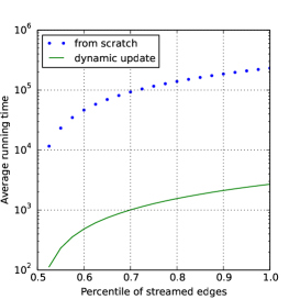
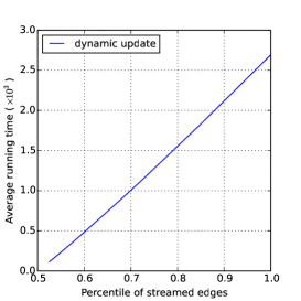
Figure 1: Running time comparisons on LiveJournal, between maintaining reverse push using Algorithm 3
and computing reverse push from scratch for every edge insertion with .
We take 100 random test nodes and compute the average running time for each algorithm.
4.3 Comparison to random walks
We compare LazyFwdUpdate and RandomWalk for the problem of finding top-K vertices ranked by their
personalized Pagerank from a source vertex.
We sample 100 test vertices uniformly at random.
For each test vertex, the correct top-K solution is the set of K vertices with highest personalized
Pagerank from that vertex.
The performance of each algorithm is measured by:
•
Accuracy: the number of correctly identified vertices (among
its computed K vertices with highest personalized Pagerank) divided by K.
•
Running time: the amount of time to maintain/update the data structures.
•
Storage: to compare storage used by RandomWalk, we multiply the number of random walks
by the expected length of a walk ( in our experiment) times 4 (number of bytes to store an integer vertex ID).
111To allow for efficient update, it’s necessary to build an inverted index for each vertex
that quickly finds to the set of random walks crossing it.
In our implementation we built a hashmap for this purpose,
resulting in an additional factor of in the amount of storage used.
Since there might be more efficient implementation, we do not take this additional factor into account
in our comparison.
For LazyFwdUpdate,
we multiply the number of nonzero estimates and residuals by 8 (number of bytes to store a pair of integer and floating point number).
Table 3 and 4 below describe the results with being 50 and 100, respectively.
We take the average of running time and storage,
and median of accuracy over the 100 sampled vertices.
For the problem of identifying top-50 nodes,
we found that RandomWalk uses 4.5 to 12 times as much storage compared to LazyFwdUpdate,
and uses 1.6 to 2.7 as much running time.
On Orkut graph, when accuracy is controlled to be at the same level as RandomWalk for LazyFwdUpdate (with ),
the average amount of storage becomes and the average running time becomes .
When is 100, the test results are qualitatively consistent with the above conclusion.
4.4 Evaluation of dynamic reverse push algorithm
In this section we evaluate the performance of our dynamic reverse push algorithm.
We compare our proposed solution (Algorithm 3) to the baseline,
where we recompute reverse push from scratch after every edge insertion using Algorithm 2.
We sample 100 target vertices uniformly at random and take the average of the running time
over these 100 samples.
We have chosen the maximum residual parameter so that at the end of
the edge stream, the median error over the 100 samples between the maintained reverse push estimates
and the true values is less than .
Because it takes too long to compute reverse push from scratch after every edge insertion for 100 sampled vertices,
we only computed reverse push from scratch for the first 1000 edge insertions.
We take the average running time for performing reverse push during 1000 edge updates,
and use this average value times the number of inserted edges as an approximation
to the true running time, if we have computed reverse push from scratch for every edge insertion.
Figure 1 shows the experiment result on the LiveJournal graph.
We found that our approach is 100x faster than the baseline.
The aggregate running time for updating reverse push has a linear correlation with the number of edges added.
This is consistent with the theoretical bound from Theorem 5.
5 Future work
In this work we presented an approach to obtain and analyze dynamic
local push algorithms.
We mention several questions that are worth further study.
In the submitted version we proposed an algoirthm that only uses random walk samples
to compute personalized PageRank between a source and a target node for undirected graphs,
but mistakenly claimed that its time complexity is the same as the state of the art [16].
It is interesting to see if such an algorithm exists or not.
Secondly, in practice, some graphs cannot fit into one machine, and it would
be interesting to see how push algorithms perform versus random
walk algorithms in such a distributed setting.
Another question is whether one can obtain an error analysis of the forward push
algorithm on a directed graph.
Understanding such an issue can be helpful for applying it in practice as well.
Acknowledgement
Research supported by the DARPA GRAPHS program via grant
FA9550-12-1-0411, and by NSF grant 1447697.
References
[1]
Reid Andersen, Christian Borgs, Jennifer Chayes, John Hopcraft, Vahab S
Mirrokni, and Shang-Hua Teng.
Local computation of pagerank contributions.
In Algorithms and Models for the Web-Graph, pages 150–165.
Springer, 2007.
[2]
Reid Andersen, Fan Chung, and Kevin Lang.
Local graph partitioning using pagerank vectors.
In Foundations of Computer Science, 2006. FOCS’06. 47th Annual
IEEE Symposium on, pages 475–486. IEEE, 2006.
[3]
Konstantin Avrachenkov, Nelly Litvak, Danil Nemirovsky, and Natalia Osipova.
Monte carlo methods in pagerank computation: When one iteration is
sufficient.
SIAM Journal on Numerical Analysis, 2007.
[4]
Lars Backstrom and Jure Leskovec.
Supervised random walks: predicting and recommending links in social
networks.
In Proceedings of the fourth ACM international conference on Web
search and data mining. ACM, 2011.
[5]
Bahman Bahmani, Abdur Chowdhury, and Ashish Goel.
Fast incremental and personalized pagerank.
Proceedings of the VLDB Endowment, 4(3):173–184, 2010.
[6]
Shumeet Baluja, Rohan Seth, D Sivakumar, Yushi Jing, Jay Yagnik, Shankar Kumar,
Deepak Ravichandran, and Mohamed Aly.
Video suggestion and discovery for youtube: taking random walks
through the view graph.
In Proceedings of the 17th international conference on World
Wide Web, pages 895–904. ACM, 2008.
[7]
Pavel Berkhin.
Bookmark-coloring algorithm for personalized pagerank computing.
Internet Mathematics, 3(1):41–62, 2006.
[8]
Soumen Chakrabarti.
Dynamic personalized pagerank in entity-relation graphs.
In Proceedings of the 16th international conference on World
Wide Web, pages 571–580. ACM, 2007.
[9]
Dániel Fogaras, Balázs Rácz, Károly Csalogány, and
Tamás Sarlós.
Towards scaling fully personalized pagerank: Algorithms, lower
bounds, and experiments.
Internet Mathematics, 2005.
[10]
David F Gleich.
Pagerank beyond the web.
SIAM Review, 57(3):321–363, 2015.
[11]
Pankaj Gupta, Ashish Goel, Jimmy Lin, Aneesh Sharma, Dong Wang, and Reza Zadeh.
Wtf: The who to follow service at twitter.
In Proceedings of the 22nd international conference on World
Wide Web. International World Wide Web Conferences Steering Committee, 2013.
[12]
Taher H Haveliwala.
Topic-sensitive pagerank: A context-sensitive ranking algorithm for
web search.
Knowledge and Data Engineering, IEEE Transactions on,
15(4):784–796, 2003.
[13]
Glen Jeh and Jennifer Widom.
Scaling personalized web search.
In Proceedings of the 12th international conference on World
Wide Web. ACM, 2003.
[14]
Peter Lofgren.
On the complexity of the monte carlo method for incremental pagerank.
Information Processing Letters, 114(3):104–106, 2014.
[15]
Peter Lofgren.
Efficient algorithms for personalized pagerank.
arXiv preprint arXiv:1512.04633, 2015.
[16]
Peter Lofgren, Siddhartha Banerjee, and Ashish Goel.
Bidirectional pagerank estimation: From average-case to worst-case.
In Algorithms and Models for the Web Graph, pages 164–176.
Springer, 2015.
[17]
Peter Lofgren, Siddhartha Banerjee, and Ashish Goel.
Personalized pagerank estimation and search: A bidirectional
approach.
In WSDM, 2016.
[18]
Peter A Lofgren, Siddhartha Banerjee, Ashish Goel, and C Seshadhri.
Fast-ppr: Scaling personalized pagerank estimation for large graphs.
In Proceedings of the 20th ACM SIGKDD international conference
on Knowledge discovery and data mining, pages 1436–1445. ACM, 2014.
[19]
Ioannis Mitliagkas, Michael Borokhovich, Alexandros G Dimakis, and Constantine
Caramanis.
Frogwild!: fast pagerank approximations on graph engines.
Proceedings of the VLDB Endowment, 8(8):874–885, 2015.
[20]
Naoto Ohsaka, Takanori Maehara, and Ken-ichi Kawarabayashi.
Efficient pagerank tracking in evolving networks.
In Proceedings of the 21th ACM SIGKDD International Conference
on Knowledge Discovery and Data Mining, pages 875–884. ACM, 2015.
[21]
Lawrence Page, Sergey Brin, Rajeev Motwani, and Terry Winograd.
The pagerank citation ranking: bringing order to the web.
1999.
[22]
Jaewon Yang and Jure Leskovec.
Defining and evaluating network communities based on ground-truth.
In Proceedings of the ACM SIGKDD Workshop on Mining Data
Semantics, page 3. ACM, 2012.