Analysis of the Intrinsic Mid-Infrared L$bandtoVisible--Near-InfraredFluxRatiosinSpectralSynthesisModelsofCompositeStellarPopulations$

Abstract

We analyze the intrinsic flux ratios of various visible–near-infrared filters with respect to 3.5 µm for simple and composite stellar populations (CSPs), and their dependence on age, metallicity, and star formation history (SFH). UV/optical light from stars is reddened and attenuated by dust, where different sightlines across a galaxy suffer varying amounts of extinction. Tamura et al. (2009) developed an approximate method to correct for dust extinction on a pixel-by-pixel basis, dubbed the “$\beta_{V}$” method, by comparing the observed flux ratio to an empirical estimate of the intrinsic ratio of visible and $\sim$3.5 µm data. Through extensive modeling, we aim to validate the “$\beta_{V}$” method for various filters spanning the visible through near-infrared wavelength range, for a wide variety of simple and CSPs. Combining Starburst99 and BC03 models, we built spectral energy distributions (SEDs) of simple (SSP) and composite (CSP) stellar populations for various realistic SFHs, while taking metallicity evolution into account. We convolve various 0.44–1.65 µm filter throughput curves with each model SED to obtain intrinsic flux ratios $\beta_{\lambda,0}$. When unconstrained in redshift, the total allowed range of $\beta_{V\!,0}$ is 0.6–4.7, or almost a factor of eight. At known redshifts, and in particular at low redshifts ($z$ $\lesssim$ 0.01), $\beta_{V\!,0}$ is predicted to span a narrow range of 0.6–1.9, especially for early-type galaxies (0.6–0.7), and is consistent with observed $\beta_{V}$ values. The $\beta_{\lambda}$ method can therefore serve as a first-order dust-correction method for large galaxy surveys that combine JWST (rest-frame 3.5µm) and HST (rest-frame visible–near-IR) data.

Published on The Astrophysical Journal

1 Introduction

Spectral energy distribution (SED) information across a wide frequency range can be used to infer the nature of the emitting source, and simultaneously the effect of the intervening interstellar medium (ISM) along the line of sight (e.g., Lindblad 1941; Elmegreen 1980; Walterbos & Kennicutt 1988; Waller et al. 1992; Witt et al. 1992; Calzetti et al. 1994; Boselli et al. 2003; Deo et al. 2006). Dust in the ISM of galaxies effectively scatters or absorbs light at shorter wavelengths, such as ultraviolet (UV) and visible photons, and reradiates the absorbed energy in the far-infrared (far-IR) (e.g., Buat & Xu 1996; Charlot & Fall 2000; Dale et al. 2001; Bell et al. 2002; Panuzzo et al. 2003; Boissier et al. 2004; Buat et al. 2005). Accordingly, dust transforms the shape of the galaxy SEDs, making it harder to study the intrinsic properties of astronomical sources (e.g., Trumpler 1930; Mathis et al. 1977; Viallefond et al. 1982; Caplan & Deharveng 1985,1986; Roussel et al. 2005; Driver et al. 2008).

In order to directly account for the transformation of the SED by dust, it would be especially helpful to have UV data accompanied by far-IR data (25–350 µm) at the same angular resolution (Calzetti et al. 2000; Bell et al. 2002; Boselli et al. 2003; Boissier et al. 2004; Buat et al. 2005). The Earth’s atmosphere, however, is mostly opaque to the far-IR (Elsasser 1938), necessitating the use of space telescopes like IRAS (Neugebauer et al. 1984), ISO (Kessler et al. 1996), Spitzer (Werner et al. 2004), and Herschel (Pilbratt 2004). Even then, it is challenging to build and operate far-IR detectors, and for a given telescope aperture, the spatial resolution is $\sim$40–800 times worse than in the optical (Xu & Helou 1996; Price et al. 2002). For these reasons, shorter wavelength data have been used in various ways to correct for extinction by dust in many studies (e.g., Lindblad 1941; Rudy 1984; Calzetti et al. 1994; Petersen & Gammelgaard 1997; Meurer et al. 1999; Scoville et al. 2001; Bell et al. 2002; Kong et al. 2004; Maíz-Apellániz et al. 2004; Calzetti et al. 2005; Relaño et al. 2006; Kennicutt et al. 2009), each with their own advantages and disadvantages (see, e.g., Tamura et al. 2009).

Tamura et al. (2009; hereafter T09) developed a simple, approximate, dust-correction method, dubbed the “$\beta_{V}$” method, which uses photometry in two broadband filters at optical ($\lambda$ $>$ 4000Å) and mid-infrared (mid-IR) $L$-band ($\sim$3.5 µm) rest-frame wavelengths, respectively. The $\beta_{V}$ method is primarily intended for the study of large numbers of spatially resolved galaxies at low to intermediate redshifts (0.1 $\lesssim$ $z$ $\lesssim$ 2), for which multiwavelength observations are too expensive and approximate dust corrections may still present a marked improvement over ignoring the effects of extinction altogether, or over adopting a single number as a canonical extinction value for a given galaxy. In particular, T09 and Tamura et al. (2010) applied the $\beta_{V}$ method to one nearby late-type spiral galaxy, NGC 959, by using $V$-band images obtained from the ground with the Vatican Advanced Technology Telescope and 3.6 µm images from space with the Spitzer/InfraRed Array Camera (IRAC), and using ancillary far- and near-UV images from the Galaxy Evolution Explorer (GALEX) in order to better distinguish pixels dominated by younger stellar populations from those dominated by older ones. From an analysis of the histogram of the observed pixel flux ratios, they adopted values of 1.10 for “older” pixels and 1.32 for “younger” pixels for the extinction-free $V$ to 3.6 µm flux ratio, $\beta_{V\!,0}$. By doing so, they were able to map the extinction across NGC 959, and obtain extinction-corrected images in which they discerned a hitherto unrecognized stellar bar. The $\beta_{V\!,0}$ values that they used for “older” pixels were consistent with the 0.5 $\lesssim$ $\beta_{V\!,0}$ $\lesssim$ 2 derived from the theoretical SED models for simple stellar populations (SSPs) of Anders & Fritze-von Alvensleben (2003). The $\beta_{V\!,0}$ values for “younger” pixels, on the other hand, were significantly smaller than those expected from theory (4 $\lesssim$ $\beta_{V\!,0}$ $\lesssim$ 7). The authors argued that blending of light from underlying and neighboring older stellar populations was the likely origin of this discrepancy. This effect will be resolution dependent and hence redshift dependent, because poor spatial resolution will mix the light from a larger area within a galaxy. To address the impact of these issues, quantitative analysis of both the effect of blending of the light from different stellar populations and of the effects of spatial resolution on extinction estimates will be necessary.

As part of a larger project to investigate the validity, robustness, and limits of the $\beta_{V}$ method (Jansen et al. 2017, in preparation), we construct SED models for stellar populations with various metallicities, ages, and star formation histories (SFHs), in order to quantify how the intrinsic optical to mid-IR flux ratio, $\beta_{\lambda,0}$, will vary. The result will be relevant, particularly, for future surveys of intermediate-redshift ($z$ $\lesssim$ 2) galaxies that combine images from the James Webb Space Telescope (JWST; Gardner et al. 2006) and the Hubble Space Telescope (HST) at rest-frame $\sim$3.5µm and visible–near-IR wavelengths, respectively. As the spatial resolution ($\propto$ $\lambda/D$) of images from JWST/NIRCam at 3.5µm will be comparable to that of HST/ACS WFC and WFC3 UVIS in $V$ to within a factor 2.5, an unprecedented detailed study of galaxies over the past 4.4 Gyr, virtually unhampered by extinction, will become possible when the $\beta_{V}$ method proves valid.

This paper is organized as follows: in §2 we explain how we combine the results of two different stellar population synthesis codes published in the literature, and how we use our adopted SSP SEDs to generate SEDs of composite stellar populations (CSPs). In §3, for different SFHs, we present $\beta_{\lambda,0}$ values obtained by convolving the SEDs with various sets of filters. In §4 we analyze and evaluate the $\beta_{\lambda}$ method as a dust-correction method. We briefly summarize in §5.

We adopt the Planck 2015 (Planck Collaboration et al. 2016) cosmology with ($H_{0}$ = 67.8 km sec^-1 Mpc^-1; $\Omega_{m}$ = 0.308; $\Omega_{\Lambda}$ = 0.692), and we will use AB magnitudes (Oke 1974; Oke & Gunn 1983) throughout.

2 SED Models

2.1 Combining the SSP Model SEDs of Starburst99 and BC03

The first step of our computational analysis is to build a large family of SSP model SEDs. Each SSP represents a single generation of stars of the same age and chemical composition, with stellar masses that were distributed according to an adopted initial mass function (IMF; Salpeter 1955; Kroupa 2002; Chabrier 2003) at birth. There are several stellar population synthesis codes available in the literature (e.g., Fioc & Rocca-Volmerange 1997; Leitherer et al. 1999; Bruzual & Charlot 2003; Maraston 2005; Vazdekis et al. 2010). We select Starburst99 (Leitherer et al. 1999 and Vázquez & Leitherer 2005) for very young ($\lesssim$30 Myr) stellar populations, since the stellar evolutionary tracks of the Geneva group (Schaller et al. 1992; Charbonnel et al. 1993; Schaerer et al. 1993a, 1993b; Meynet et al. 1994) adopted by Starburst99 are optimized for massive young stars, and include, e.g., the Wolf-Rayet phase. Starburst99 also includes nebular continuum from the gas enshrouding the stellar populations, as is the general case for newborn and young stars. On the other hand, the stellar evolutionary tracks of the Padova group (Girardi et al. 2000; Marigo et al. 2008) are a good match to observations of intermediate- and low-mass stars that dominate older stellar populations (Vázquez & Leitherer 2005). We therefore adopt the Padova1994 tracks in BC03 (Bruzual & Charlot 2003) for older ($\gtrsim$100 Myr) stellar populations. Below, we describe how we combine the two sets of SED models into a database that can be used for stellar populations of any age. The age grid of the BC03 code is fixed as 221 logarithmic steps between 10⁵ and 10¹⁰ years. In the Starburst99 code, however, the user can specify the age step and scale, so we set 1000 logarithmic time steps between 10⁶ and 10¹⁰ years in order to provide a finer grid than BC03. For both codes, we adopted a Salpeter (1955) stellar IMF, with a power-law slope of $-$2.35, and with minimum and maximum stellar masses of 0.1 and 100 $\textrm{M}_{\odot}$. Each code has a different set of metallicities: $Z$ = 0.001, 0.004, 0.008, 0.02, and 0.04 for Starburst99 and $Z$ = 0.0001, 0.0004, 0.004, 0.008, 0.02, and 0.05 for BC03. We extrapolate the Starburst99 SEDs to match the metallicities of BC03 using the method described in the following. For each code, we log-exponentially extrapolated in $[Z]$ = $\log_{10}(Z/Z_{\odot})$ (where $Z_{\odot}$ $=$ 0.02) from the two SEDs that are closest in metallicity to the desired value. For example, to obtain our $Z$ = 0.0004 SED in Starburst99, we combined SEDs for $Z$ = 0.001 and $Z$ = 0.004 in Starburst99 with relative weights of 1.40 and $-$0.40, which are derived from $F_{1}$ = $(F_{2}-w\cdot F_{3})/(1-w)$, where $F_{1}$, $F_{2}$, and $F_{3}$ denote the logarithm of the wavelength-dependent flux densities of SEDs with metallicities of $Z_{1}$, $Z_{2}$, and $Z_{3}$ (with $Z_{1}$$<$$Z_{2}$$<$$Z_{3}$), and where the weight $w$ = $(e^{Z_{2}}-e^{Z_{1}})/(e^{Z_{3}}-e^{Z_{1}})$. Similarly, when interpolating $F_{2}$ into $F_{1}$ and $F_{3}$, we use $F_{2}=(1-w)\cdot F_{1}+w\cdot F_{3}$. Note that the SEDs $F_{1}$, $F_{2}$, and $F_{3}$ and metallicities $Z_{1}$, $Z_{2}$, and $Z_{3}$ are in log scale, with the latter all known (e.g., 0.0004, 0.001, and 0.004 giving $w$ $=$ 0.285 in our example).

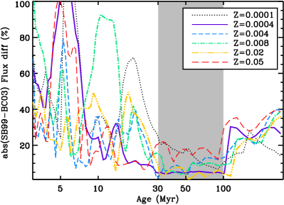
Figure 1: Integrated absolute flux difference over the 0.4–3.75 µm wavelength range between Starburst99 and BC03 SEDs (see Eq. 1) as a function of SSP age for various metallicities. There is no specific age where both codes converge on an identical SED, but the percentage difference reaches a general minimum between $\sim$30 and $\sim$100 Myr, where they are mostly $\lesssim$10$\%$.

Table 1: Transition age range adopted when combining Starburst99 and BC03 stellar population synthesis model SEDs for various metallicities, $Z$. Minimum, maximum, and mean relative flux differences of the two SEDs in the transition age range, and rms thereof are also tabulated.

$Z$	Age range	Min. Diff.	Max. Diff.	Mean Diff.	RMS
	(Myr)	(%)	(%)	(%)	(%)
0.0001	30–100	7	25	17	5.0
0.0004	30–100	4	5	5	0.3
0.004	30–100	2	13	7	3.0
0.008	30–100	4	15	8	3.3
0.02	30–100	1	9	5	2.1
0.05	30–100	11	22	17	3.2

For intermediate ages (30 $\lesssim$ Age $\lesssim$ 100 Myr), we interpolate the results of the two codes onto the BC03 Age grid as follows. To minimize discontinuities and sudden changes of SEDs for intermediate ages, we inspected the integrated absolute flux differences between Starburst99 and BC03 SEDs over the 0.4–3.75 µm wavelength range (the relevant range for the $\beta_{V}$ method; see T09). This quantity is for a given age given by:

$$\frac{\int_{\lambda_{1}}^{\lambda_{2}}{\bigl{|}F_{SB99}(\lambda)-F_{BC03}(\lambda)\bigr{|}}}{\text@frac{1}{2}\left(\int_{\lambda_{1}}^{\lambda_{2}}{F_{SB99}(\lambda)}+\int_{\lambda_{1}}^{\lambda_{2}}{F_{BC03}(\lambda)}\right)},$$ (1)

with ($\lambda_{1}$, $\lambda_{2}$) = (0.4, 3.75) µm, and its dependence on age and metallicity is shown in Figure 1. Table 1 lists the minimum, maximum, mean, and rms differences. At 30 Myr, 100% of the Starburst99 SED and 0% of the BC03 SED is used, and the contributions are linearly reduced (increased) to 0% (100%) at 100 Myr. Interpolating using $\log($Age$)$ instead of Age yields nearly identical results, since the age ranges are relatively narrow.

Figure 2 shows examples of our combined SSP SEDs for six metallicities and 16 ages. We use this set of ages and metallicities when we calculate the $L$ band to visible–near-IR flux ratios of stellar populations with various SFHs described in §3. We also use the same parameter set when we select a manageably small but comprehensive set of SSP SEDs, which we extend with additional extinction-related parameters in Appendix A.

      

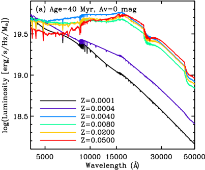
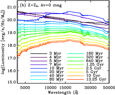
Figure 2: Examples of our adopted combined array of SSP SEDs. (a) SEDs for a 40 Myr old stellar population, for six different metallicities and no extinction; (b) SEDs for 16 different ages with fixed solar metallicity ($Z_{\odot}$ = 0.02) and zero extinction.

2.2 SFH, Metallicity Evolution, and Construction of CSP SEDs

Whereas an SSP consists of purely coeval stars, realistic star formation within galaxies is characterized by stochastic and/or temporally extended, possibly spatially propagating, episodes of star formation. The CSP of a larger region within a galaxy therefore effectively records its SFH. If we denote that SFH as the time-dependent star formation rate, $\psi(t)$, and the SED of an SSP as a function of its age, $t$, and metallicity, $Z$, by $F_{\lambda,{\rm SSP}}(t,Z)$, then we can express the SED of a CSP as the superposition of multiple SSPs:

$$F_{\lambda,{\rm CSP}}(t,Z)=\sum_{t^{\prime}=t_{0}}^{t}{F_{\lambda,{\rm SSP}}(t-t^{\prime}\!,Z(t^{\prime}))\,\psi(t^{\prime})\,\delta t^{\prime}}\,,\$$ (2)

where $F_{\lambda,{\rm SSP}}$ is derived by interpolating our combined SSP SEDs to generate a set of SEDs with 28 logarithmic steps in metallicity (between $Z$ = 0.0001 and $Z$ = $0.05$) and 1000 logarithmic steps in Age (between $t$ = 1 Myr and $t$ = 13.8 Gyr), $Z(t^{\prime})$ is used to explicitly denote the time-dependence of the metallicity, and $t_{0}$ denotes the time of the first episode of star formation. The metallicity at time step $t^{\prime}$ results from metal-enriched gas returned to the ISM by stars from previous generations of stellar populations, and from accretion of gas from other nearby galaxies or from the IGM and circum-galactic medium (whether more enriched, or diluted) by the end of time step $(t-\delta t)$. Note that this implies that the metallicity of the resulting CSP differs from that of the metallicity of (most of) its constituent SSPs, and that the chemical evolution of the CSP will not be entirely self-consistent with the choice of the SFH. It does account, however, for the open-box, rather than closed-box, nature of a galaxy or galaxy region in an empirical way. We return to the functional form of $Z(t^{\prime})$ shortly.

Figure 3: Examples of five arbitrary scenarios of stochastic SFHs. Relative star formation rates ($\psi$, normalized to the peak of the strongest star formation episode) are plotted as a function of cosmic time (bottom axis) and redshift (top axis) in both linear (solid curves; left axis) and logarithmic (dotted; right axis) units. SFH1 and 2 represent the cases of two and three bursts with long (1 Gyr) and shorter (0.5 Gyr) $e$-folding times, respectively. SFH3, 4, and 5 represent simulated CSPs of early-type (E,S0), spiral (Sa–Sbc) and late-type (Sc,Sd) galaxies, respectively.

     

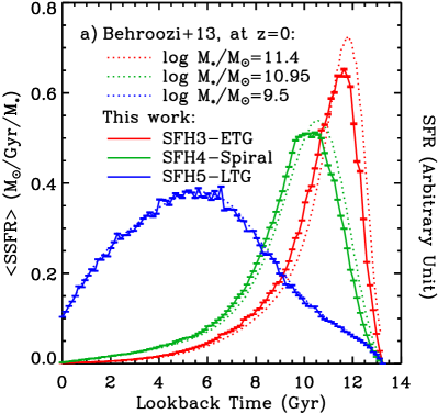
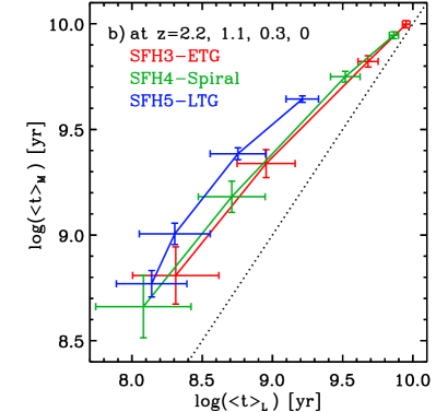
Figure 4: (a) Specific SFR versus lookback time for our families of stochastic SFHs. We show the mean and standard deviation of the mean SFR normalized by the total stellar mass built up at $z$ = 0 for 1000 random realizations each of SFH3, SFH4, and SFH5 (solid distributions). The dotted curves represent the models of Behroozi et al. (2013) for present-day stellar masses of 2.5$\times$10¹¹, 8.9$\times$10¹⁰, and 3.1$\times$10⁹ $\textrm{M}_{\odot}$, representative of early-type (E), spiral (Sb), and late-type (Sd) galaxies, respectively. (b) Mean and scatter of the light- and mass-weighted ages of our stochastic SFHs at redshifts of 0 (upper right), 0.3, 1.1, and 2.2 (lower left). The mass-weighted ages are always larger than the light-weighted ones, but the gap between them decreases from redshift $z$ = 2 to the present ($z$ = 0).

We started by building CSP SEDs for stellar populations with exponentially declining star formation rates, $\psi(t)$ = $\psi_{0}$ ${e^{-t/\tau}}$ for various values of the $e$-folding time $\tau$ (100, 250, 500 Myrs, 1, 2, 5, and 10 Gyr, where the latter two approach the case of a constant star formation rate). Note that for these exponentially declining SFHs, which were merely meant to test the effect of combining SSPs of different ages, we did not yet take metallicity evolution into account. We then produced SEDs for more realistic stochastic SFHs, built from multiple partially overlapping exponentially declining starbursts with onset times $t_{0,i}$, $e$-folding time $\tau_{i}$, and peak amplitude $\psi_{0,i}$ from

$$\psi(t)=\sum_{i}^{n}\psi_{0,i}\,e^{-(t-t_{0,i})/\tau_{i}}\;.$$ (3)

We adopt five different families of stochastic SFHs (five examples of which are shown in Figure 3). SFH1 and SFH2 are simple test cases with $n$ = 2 long ($\tau_{i}$ = 1 Gyr) and $n$ = 3 short ($\tau_{i}$ = 100 Myr) bursts, respectively. For each of SFH3, SFH4, and SFH5 we randomly generated 1000 stochastic composite SFHs by combining multiple exponentially declining starbursts with different constraints in order to simulate galaxies of different (Hubble) types and present-day stellar masses. For SFH3, we restrict $e$-folding times $\tau_{i}$ to 50 Myr $<$ $\tau_{i}$ $<$ 1 Gyr, for SFH4 100 Myr $<$ $\tau_{i}$ $<$ 500 Myr, and for SFH5 to 5 Myr $<$ $\tau_{i}$ $<$ 100 Myr, representative of likely starbursts in early-type, spiral, and late-type galaxies. The mean $e$-folding times are $\sim$300 Myr, $\sim$250 Myr, and $\sim$30 Myr, respectively. We then estimate the number of starburst episodes required for each SFH family by dividing the Hubble time (13.8 Gyr) by these mean $e$-folding times, giving 44, 53, and 427 for SFH3, SFH4, and SFH5.

We furthermore adopt the model SFHs of Behroozi et al. (2013) to define constraints for our mean starburst amplitudes $\psi_{0,i}$ as a function of time of onset $t_{0,i}$. We chose model SFHs resulting in present-day stellar masses of 2.5$\times$10¹¹, 8.9$\times$10¹⁰, and 3.1$\times$10⁹ $\textrm{M}_{\odot}$ ($\log(\textrm{M}/\textrm{M}_{\odot})$ of 11.4, 10.95, and 9.5) for SFH3, SFH4, and SFH5, respectively, to match the distribution of stellar masses for Hubble types E, Sb, and Sd found by González-Delgado et al. (2015; hereafter GD15) in the CALIFA IFU survey of 300 local galaxies (see their Figure 2). Figure 4(a) compares the mean specific star formation rates as a function of lookback time for each of our SFH families and for the corresponding Behroozi et al. (2013) models. For SFH3, we find that the results shown in Figure 4(a) are sensitive to the choice of lower bound on $\tau_{i}$, such that for longer minimum burst durations we would fail to reproduce the steep rise and relatively fast decline in SF for massive (early-type) galaxies in the Behroozi et al. (2013) models. The resulting SF peak is reached at $z$ = 3.0 for SFH3, at $z$ = 2.1 for SFH4, and at $z$ = 0.6 for SFH5.

Table 2: Log-linear metallicity evolution parameters, fit to the results of Maiolino et al. (2008) combined with our stochastic SFHs. We approximate that evolution by $\log{Z(z)}=a\cdot z+b$. The rms of the fit in each of $a$ and $b$ is $<$0.01. We adopt the slopes in parentheses: $-$0.18 for SFH3, $-$0.30 for SFH4, and $-$0.58 for SFH5.

$\log\mathrm{M}/\mathrm{M}_{\odot}$	SFH3-ETG		SFH4-Spiral		SFH5-LTG
	$a$	$b$	$a$	$b$	$a$	$b$
9.50	$-$0.37	0.25	$-$0.49	0.29	($-$0.58)	0.22
10.95	$-$0.23	0.49	($-$0.30)	0.52	$-$0.36	0.50
11.40	($-$0.18)	0.49	$-$0.24	0.52	$-$0.30	0.51

For all CSPs constructed as described above, the normalization of the SFH is such that $\sum\psi(t^{\prime})\delta t^{\prime}$ = M, the total mass in stars formed up to the present time, which will be higher than the current stellar mass because of mass returned by stellar winds and supernova explosions, but by no more than $\sim$30% (see Vázquez & Leitherer 2005). The more recent SF in low-mass (late-type) galaxies, i.e., downsizing, results in younger ages, especially light-weighted ages (see Figure 4(b)). Mass-weighted ages are always larger than light-weighted ones, but Figure 4(b) shows that the gap between them decrease from a factor of 3 at $z$ = 2 to $\sim$10% at $z$ = 0 for SFH3 and SFH4. For SFH5, the difference remains a factor of $\sim$5 until $z$ $\sim$ 0.3 before decreasing to a factor of $\sim$3 at $z$ $\simeq$ 0.

To account for metallicity evolution and arrive at a functional form for $Z(t^{\prime})$ in Eq. 2, we combine our stochastic SFHs with the mass-metallicity relations at $z$ $\simeq$ 0, 0.3, 1.1, and 2.2 presented by Maiolino et al. (2008). At $z$ = 0, we assume stellar masses of 2.5$\times$10¹¹, 8.9$\times$10¹⁰, and 3.1$\times$10⁹ $\textrm{M}_{\odot}$ for early-type, spiral, and late-type galaxies as above. We find that we can approximate the metallicity evolution as $\log Z(z)=a\cdot z+b$, and fit slopes $a$ for each of these present-day stellar masses and SFHs (see Table 2). We adopt $a$ = $-$0.18, $-$0.30, and $-$0.58 for the metallicity evolution of SFH3, SFH4, and SFH5, respectively. Note that while we list fitted values in the final column of Table 2 for SFH5 for each of our three stellar masses, late-type galaxies with M $>$ 10¹⁰ are extremely rare in nature (e.g., Kelvin et al. 2014).

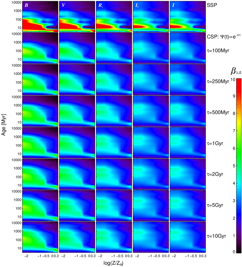
Figure 5: Maps of $\beta_{\lambda,0}$ values referenced to the Johnson $L$ band as a function of metallicity ($Z/Z_{\odot})$ and age of the stellar populations for the (left to right) Johnson $B$, $V\!$, Kron-Cousins-Glass $R_{c}$, $I_{c}$, and Johnson $I$ filters for (top to bottom) SSPs, and for seven composite stellar populations resulting from exponentially declining SFHs with $\tau$ = 100, 250, 500 Myr, 1, 2, 5, and 10 Gyr. Maps of $\beta_{\lambda,0}$ values for our full set of visible–near-IR filters are available as Figure Set 5 in the electronic edition of the journal or at the end of this paper.
(The complete figure set (seven images) is available.)

Table 3: The mean, standard deviation, minimum and maximum of $\beta_{V\!,0}$ values inferred for our SSPs and CSPs with exponentially declining SFHs (2nd column in Figure 5) for all $Z$, and separately for $Z$=0.004, $Z$=0.008, and $Z$ = $Z_{\odot}$ = 0.02, respectively.

SFH	0.0001 $\leq$ $Z$ $\leq$ 0.05			$Z$ = 0.004			$Z$ = 0.008			$Z$ = 0.02
	$\langle$$\beta_{V\!,0}$$\rangle$	Min	Max	$\langle$$\beta_{V\!,0}$$\rangle$	Min	Max	$\langle$$\beta_{V\!,0}$$\rangle$	Min	Max	$\langle$$\beta_{V\!,0}$$\rangle$	Min	Max
SSP	3.84$\pm$3.57	0.10	23.64	3.06$\pm$2.10	1.03	8.99	2.41$\pm$1.65	0.73	7.79	2.06$\pm$1.67	0.37	7.77
$\tau$=100 Myr	2.74$\pm$1.37	0.35	6.05	2.67$\pm$1.22	1.04	4.71	2.13$\pm$0.89	0.73	3.89	1.86$\pm$0.92	0.55	4.13
$\tau$=250 Myr	2.80$\pm$1.36	0.35	5.88	2.75$\pm$1.20	1.04	4.67	2.18$\pm$0.87	0.73	3.87	1.90$\pm$0.90	0.55	4.11
$\tau$=500 Myr	2.85$\pm$1.35	0.35	5.82	2.82$\pm$1.17	1.04	4.65	2.22$\pm$0.85	0.73	3.86	1.93$\pm$0.84	0.56	4.11
$\tau$=1 Gyr	2.92$\pm$1.33	0.36	5.78	2.88$\pm$1.13	1.04	4.64	2.26$\pm$0.82	0.74	3.86	1.97$\pm$0.84	0.56	4.10
$\tau$=2 Gyr	2.98$\pm$1.29	0.37	5.77	2.95$\pm$1.06	1.06	4.64	2.31$\pm$0.76	0.77	3.86	2.02$\pm$0.79	0.59	4.10
$\tau$=5 Gyr	3.05$\pm$1.24	0.48	5.76	3.02$\pm$0.98	1.24	4.64	2.37$\pm$0.69	0.96	3.86	2.07$\pm$0.73	0.76	4.10
$\tau$=10 Gyr	3.08$\pm$1.22	0.57	5.75	3.05$\pm$0.95	1.38	4.64	2.39$\pm$0.66	1.11	3.85	2.09$\pm$0.70	0.89	4.10

3 Intrinsic $\beta_{\lambda,0}$ Flux Ratios from Model SEDs

T09 developed the $\beta_{V}$ method to estimate the amount of dust extinction in a galaxy using images through just two broadband filters: one visible ($V$) and one in the mid-IR near 3.5 µm ($L$ band), specifically, Spitzer/IRAC 3.6 µm in their case. The $L$ band is where the extinction by dust reaches a minimum, and where there is still little emission from warm dust, polycyclic aromatic hydrocarbons (PAHs), and silicates (although there is a significant C–H stretching PAH feature near 3.3 µm; Léger & Puget 1984; Allamandola, Tielens & Barker 1989). If we have knowledge of the intrinsic SED of a simple or CSP, then we can calculate the intrinsic flux ratio $\beta_{V\!,0}$ = $f_{V\!,0}/f_{L,0}$. This ratio will be a function of age $t$, metallicity $Z$, and SFH $\psi(t)$. If $\beta_{V\!,0}$ values were to fall in a very narrow range for a wide range of such CSP parameters, and if our model SEDs were accurate representations of observed stellar populations, then comparing the observed ($\beta_{V}$) and the intrinsic ($\beta_{V\!,0}$) flux ratios would allow us to infer the missing flux in the $V$ band. We furthermore assume that the extinction in bandpasses centered near 3.5 µm ($L$) is negligible. The extinction in magnitudes is given by $A_{V}$ = $(m_{V}-m_{V\!,0})$, which can be rewritten in terms of the observed $L$-band flux and the intrinsic $V$-to-$L$-band flux ratio $\beta_{V\!,0}$ as

$$A_{V}\simeq\ m_{V}-[-2.5\,\log\left(\beta_{V\!,0}\times f_{L}\right)-V_{\rm zp}]\ ,$$ (4)

where $f_{L}$ $\simeq$ $f_{L,0}$, $V_{\rm zp}$ is the zero-point magnitude for the $V$ filter, and the $\simeq$ -symbol serves to recall the approximate nature of this method.

Here, we consider a more general extension of the $\beta_{V}$ method, the $\beta_{\lambda}$ method, where we compute $\beta_{\lambda,0}$ for a large selection of filter pairs in the rest-frame optical ($\lambda$ $\sim$ 0.4–1 µm) and rest-frame mid-IR ($\lambda$ $\sim$ 3.4–3.6 µm). In total, 29 visible–near-IR and 5 mid-IR filter throughput curves were convolved with the simple and composite SEDs we constructed as described in §2 to obtain the $\beta_{\lambda,0}$ values for each SED.

We make all models and derived data available on our website as ASCII text tables and as 2D maps of $\beta_{\lambda,0}$($Z$,$t$) in both PNG and FITS format.

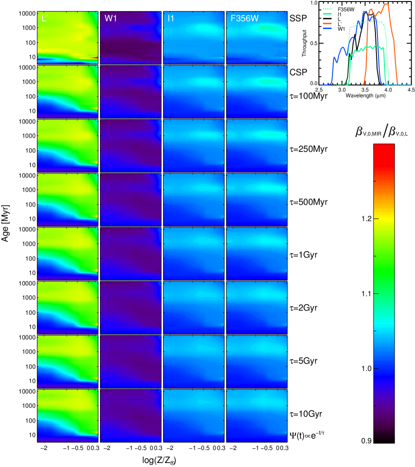
Figure 6: Maps of ratios $r_{\beta}(\mathrm{MIR},L)$ = $F(L)/F(L^{\prime})$, $F(L)/F(W\textsl{1})$, $F(L)/F(I\textsl{1})$, and $F(L)/F(\mathrm{F356W})$ as a function of metallicity ($Z/Z_{\odot})$ and age $t$ of the stellar populations and stellar population models as shown in Figure 5. $r_{\beta}(\mathrm{MIR},L)$ gradually increases as stellar populations age and decreases again for super-solar metallicity. The color bar in this figure spans a much narrower range than the one in Figure 5. For reference, we plot the throughput curves of each MIR bandpass in the inset at the upper right.

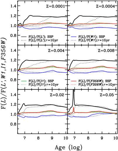
Figure 7: Flux ratios between different choices of mid-IR reference filters as a function of the age of the stellar populations for various metallicities. Solid curves are for SSPs and dotted curves are for exponentially declining SFHs with a 1 Gyr $e$-folding time. The ratio generally remains stable in the 0.9–1.2 range for ages larger than a few tens of Myr. While the $\beta_{\lambda,0}$ value to adopt depends on the choice of mid-IR reference filter, it is predictable, so any of the filters considered will be similarly valid for the application of the $\beta_{\lambda}$ method.

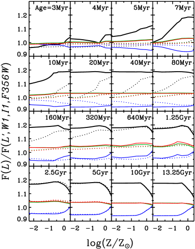
Figure 8: Flux ratios between different choices of mid-IR reference filters as a function of the metallicity of the stellar populations for various ages. Line and color schemes are the same as in Figure 7. If we exclude the red supergiants feature at ages of $\sim$5–10 Myr and high metallicity, the choice of mid-IR reference filter affects $\beta_{\lambda,0}$ at the $\lesssim$20% level, and for a given reference filter, much less than that over most of the range in age and metallicity.

3.1 SSP and Exponentially Declining SFHs

Figure 5 depicts an example of 2D maps of $\beta_{\lambda,0}$ ratios as a function of metallicity and stellar population age (or time since the onset of SF) for the Johnson $B$, $V\!$, Kron-Cousins-Glass $R_{c}$, $I_{c}$, and Johnson $I$ filter (Bessell 1990), when referenced to the Johnson $L$ band (Bessell & Brett 1988). From top to bottom, we show the results for SSPs and for seven exponentially declining SFHs with $\tau$ = 100, 250, and 500 Myr, and 1, 2, 5, and 10 Gyr. The final row approximates a continuous nearly constant star formation rate. For each panel, we started with a 2D array of SEDs that has six rows and 16 columns, corresponding to the metallicity and age values of Figure 2, for which we computed $\beta_{\lambda,0}$ values by convolving each of the filter curves with each of the 6$\times$16 SEDs. The resulting array of $\beta_{\lambda,0}$ values was expanded through log–log cubic-spline interpolation into the finer 100$\times$100 grids of metallicity and age as shown. SSPs show the highest dispersion and widest range of $\beta_{V\!,0}$ values (see Table 3). For exponentially declining SFHs, as $\tau$ increases, the standard deviations and min–max ranges decrease, while the mean $\beta_{V\!,0}$ values themselves slightly increase ($\lesssim$11%). The lower metallicity population has higher $\beta_{V\!,0}$ values as well ($\sim$50% for $Z$ $=$ 0.0004 compared to $Z$ $=$ 0.02).

Similarly, in Figure Set 5, we show $\beta_{\lambda,0}$ referenced to the same Johnson $L$ band for the SDSS $g$, $r$, $i$, and $z$ filters (Gunn et al. 1998), as well as for eight HST/ACS WFC (Ford et al. 2003; Avila et al. 2015) and eight HST/WFC3 UVIS (Dressel 2015) filters. The choice of filters was motivated by their common use for HST deep and medium-deep surveys, such as the Great Observatories Origins Deep Survey (GOODS; Dickinson et al. 2003, p. 324; Giavalisco et al. 2004), the Cosmic Assembly Near-IR Deep Extragalactic Legacy Survey (CANDELS; Grogin et al. 2011; Koekemoer et al. 2011), the Cosmological Evolution Survey (COSMOS; Scoville et al. 2007), the Cluster Lensing and Supernova Survey (CLASH; Postman et al. 2012), and the HST/WFC3 Early Release Science (ERS) program (Windhorst et al. 2011). In Figure Set 5, moreover, we extend our coverage to the near-IR with four WFC3/IR filters.

Table 4: Comparison of the mean values and standard deviations of $r_{\beta}(\mathit{MIR},L)$ = $\beta_{\lambda,0}^{\mathit{MIR}}/\beta_{\lambda,0}^{L}$ = $F(L)/F(\mathit{MIR})$, before and after 3$\sigma$ rejection, for our SSPs and CSPs with exponentially declining SFHs (first and fifth rows in Figure 6).

$\mathit{MIR}$	SSP		$\tau$=1 Gyr
	Mean	Robust mean	Mean	Robust mean
$L^{\prime}$	1.16$\pm$0.05	1.18$\pm$0.01	1.11$\pm$0.07	1.11$\pm$0.08
$W$1	0.95$\pm$0.02	0.95$\pm$0.02	0.96$\pm$0.01	0.96$\pm$0.02
$I$1	1.03$\pm$0.01	1.04$\pm$0.01	1.02$\pm$0.02	1.02$\pm$0.02
F356W	1.03$\pm$0.02	1.03$\pm$0.02	1.02$\pm$0.02	1.02$\pm$0.02

One might wonder how sensitive the $\beta_{\lambda}$ method is to the exact choice of the mid-IR reference filter. We thus considered the ground-based Johnson $L$ and $L^{\prime}$ filters, the space-based WISE $W$1 bandpass ($\lambda_{\rm eff}$ = 3.3526 µm, $\Delta\lambda$ = 0.66 µm; Wright et al. 2010; Jarret et al. 2011), the Spitzer/IRAC $I$1 bandpass ($\lambda_{\rm eff}$ = 3.550 µm, $\Delta\lambda$ = 0.75 µm; Fazio et al. 2004), and the JWST/NIRCam (Horner & Rieke 2004; Gardner et al. 2006; Rieke 2011) F356W filter ($\lambda_{\rm eff}$ = 3.568 µm, $\Delta\lambda$ = 0.781 µm). In Figure 6 and Table 4, we compare the ratios of $\beta_{\lambda,0}$ computed relative to each mid-IR (MIR) band and to the $L$ band: $r_{\beta}(\mathrm{MIR},L)$ = $\beta_{\lambda,0}^{\mathit{MIR}}/\beta_{\lambda,0}^{L}$ = $F(L)/F(\mathrm{MIR})$. The ratios get closer to unity and the range in values decreases for the exponentially declining SFHs with $\tau$ = 1 Gyr. The $\beta_{\lambda,0}$ values referenced to the $I\textsl{1}$ and F356W filters are similar to those referenced to the $L$ band, whereas $\beta_{\lambda,0}$ values referenced to $L^{\prime}$ and $W\textsl{1}$ were higher and lower, respectively. The $r_{\beta}(L^{\prime},L)$ values tend to be higher than 1 (i.e., $\beta_{\lambda,0}^{L^{\prime}}$ $>$ $\beta_{\lambda,0}^{L}$), because we are sampling the Rayleigh-Jeans tail of the stellar SED and the central wavelength of the $L^{\prime}$ filter is longer than that of the $L$ filter. Conversely, the central wavelength of the $W$1 bandpass lies shortward of that of $L$, resulting in $r_{\beta}(W\textsl{1},L)$ smaller than 1. Except for a difference in the overall throughput, the $I$1 and F356W bandpasses have very similar shapes and similar central wavelengths to the $L$ filter, as shown in the inset at the upper right side of Figure 6.

In Figure 7 we plot $r_{\beta}(L^{\prime},L)$ as a function of age for six different metallicities for SSPs (black solid curves) and for exponentially declining SFHs (black dotted curves). At low metallicities, $r_{\beta}(L^{\prime},L)$ is seen to be remarkably independent of age for ages older than 10 Myr for SSPs. For CSPs with an exponentially declining SFR and an $e$-folding time of 1 Gyr, $r_{\beta}(L^{\prime},L)$ stabilizes around 500–600 Myr. At solar metallicity and above, and particularly for SSPs, sharp features become noticeable around 10 Myr of age in both Figure 6 and 7. These features correspond to the appearance and demise of red supergiants (RSGs; Walcher et al. 2011). The strength or absence of these RSG features at low metallicity remains uncertain (see, e.g., discussions in Cerviño & Mas-Hesse 1994; Leitherer et al. 1999; Vázquez & Leitherer 2005). The flux ratios for different mid-IR filters are similar at early ages ($\sim$3 Myr), but diverge until an age of $\sim$10 Myr before stabilizing again for ages larger than 1 Gyr in the case of super-solar metallicities. This pattern is more clearly shown in Fig 8, which plots $r_{\beta}(\mathit{MIR},L)$ as a function of metallicity at 16 different ages. $r_{\beta}(\mathit{MIR},L)$ is insensitive to metallicity at most stellar population ages (the curves in Fig 8 are nearly flat for most ages $\gtrsim$10 Myr and for most sub-solar metallicities). If we exclude the RSG feature at high metallicity, the choice of mid-IR filter affects $\beta_{\lambda,0}$ at the $\lesssim$20% level overall, while reference filter-dependent variations with respect to the $L$ band are much smaller than that over most of the range in age and metallicity. One can gauge the impact of a given choice of mid-IR reference filter using Figs. 6–8.

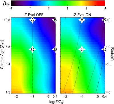
Figure 9: Comparison of $\beta_{V\!,0}$ values when metallicity evolution is (right) and is not (left) taken into account for the CSPs characterized by SFH4 (spiral galaxies). For four specific realizations of SFH4, we show the metallicity tracks as a function of cosmic age of the SSP SEDs, which are stacked to generate CSP SEDs at that age. The endpoints ($z$, $Z$) for tracks A, B, C, and D are (0.0, 0.002), (0.0, 0.05), (1.0, 0.002), and (1.0, 0.05), respectively. When we include metallicity evolution, we find a stronger dependence of $\beta_{V\!,0}$ on redshift, with higher $\beta_{V\!,0}$ values for the progenitors of present-day galaxies than in the no-evolution case.

3.2 Stochastic Multiburst SFHs

The $\beta_{V}$ method was originally developed as an approximate dust extinction correction method for large surveys of spatially resolved galaxies with unresolved stellar populations. The light from the unresolved stellar populations will have more complex SFHs than SSP or exponentially declining SFHs (Gerola & Seiden 1978; Kauffmann et al. 2006; da Silva et al. 2012). Hence, building SEDs for complex SFHs with stochastic starbursts and inspecting the resulting $\beta_{\lambda,0}$ values will be essential to determine whether the $\beta_{V}$ method (or its extension, the $\beta_{\lambda}$ method) is applicable. As mentioned in § 2.2, metallicity evolution is taken into account when we build the SED arrays for stochastic SFHs, which moves the metallicity range toward higher values when cosmic age increases and redshift decreases. When metallicity evolution is taken into account, initial metallicities for cosmic ages less than 1.5 Gyr ($z$ $>$ 4) may be below the lower limit ($Z$ = 0.0001) of our SSP model SEDs. There, our CSPs will have an artificial lower limit in metallicity of $Z$ = 0.0001, so we will not consider redshifts $z$ $>$ 4. Figure 9 shows the difference between $\beta_{V\!,0}$ values when metallicity evolution is (right) and is not (left) applied for the CSPs characterized by SFH4 (spiral galaxies; see Figure 3 and Figure 4(a)). We adopt a metallicity evolution of $-$0.30 per unit $z$, appropriate for SFH4 (see Table 2). To illustrate the effect of metallicity evolution for four specific realizations of SFH4, we show the metallicity tracks as a function of cosmic age of the SSP SEDs, which are stacked to generate CSP SEDs at that age. The effects of metallicity evolution become evident at $z$ $\gtrsim$ 1 (cosmic age $\lesssim$5.8 Gyr). For the progenitors of galaxies at a given redshift, significantly higher values of $\beta_{V\!,0}$ must be assumed at longer lookback times than in the no-evolution case, so that there is a stronger dependence of $\beta_{V\!,0}$ on redshift.

In Figure 10 we present maps of $\beta_{\lambda,0}$ as a function of cosmic age and metallicity, and 1D profiles of $\beta_{\lambda,0}$ values as a function of redshift. The $\beta_{\lambda,0}$ values without metallicity evolution are overplotted in each 1D profile panel for comparison. Each curve in the panels for SFH3, SFH4, and SFH5 represents the median $\beta_{\lambda,0}$ values of 1000 randomly generated stochastic SFHs in that family. Comparing the solid to the dotted profiles in Figure 10(b), we find that the $\beta_{\lambda,0}$($z$) values are higher when metallicity evolution is taken into account, and progressively more so for higher present-day metallicity values (at low present-day metallicities the difference must necessarily be small). The spread in $\beta_{\lambda,0}$ at a given redshift due to metallicity differences tends to be smaller than in the no-evolution case. While the range in $\beta_{\lambda,0}$ values at $z$ $\simeq$ 0 is comparable in both the evolution and no-evolution cases for each of SFH3, SFH4 and SFH5, this range becomes narrower toward higher redshifts for SHF4, and especially for SFH5. For these two SFH families, more of the stars formed relatively recently, with much (or even most) of the metallicity evolution taking place in the redshift range of interest (see our adopted slopes in Table 2). The range of $\beta_{V\!,0}$ for SFH3, SFH4, and SFH5 changes from 2.4–4.7 to 0.6–2.3 as the redshift decreases from 4 to 0. If we impose a minimal constraint on the redshift range without assuming any particular SFH family, we find allowed ranges for $\beta_{V\!,0}$ of 0.6–3.4 when 0 $<$ $z$ $<$ 1, and 0.90–3.85 when 1 $<$ $z$ $<$ 2. When the redshift is known, we find narrower ranges of 0.57–2.30, 0.70–2.93, 0.90–3.35, 1.17–3.58, and 1.52–3.85 for $\beta_{V\!,0}$ at $z$=0, 0.5, 1.0, 1.5, and 2.0, respectively. In § 3.3 we will show that these $\beta_{\lambda,0}$ ranges are further reduced once we can also constrain the range of likely SFHs and metallicities. For our full set of visible–near-IR filters, we refer the reader to Figure Set 10.

(a)  

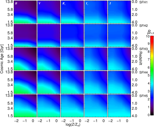
(b)  

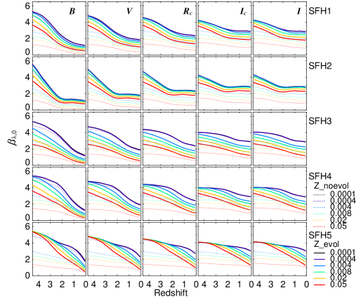
Figure 10: (a) Maps of $\beta_{\lambda,0}$ values referenced to the Johnson $L$ band as a function of metallicity ($Z/Z_{\odot})$ and cosmic age for the (left to right) Johnson $B$, $V\!$, Kron-Cousins-Glass $R_{c}$, $I_{c}$, and Johnson $I$ filters for (top to bottom) stochastic (multiburst) SFHs (see Figure 3) with metallicity evolution taken into account. (b) $\beta_{\lambda,0}$ profiles of stellar populations with various present-day ($z$$=$0) metallicities that have different stochastic SFHs as a function of redshift. For comparison, we overplot the no-evolution case (dotted curves). Each map and each curve in the panels for SFH3, SFH4, and SFH5 represents the median $\beta_{\lambda,0}$ values of 1000 randomly generated SFHs in that family. Maps and profiles of $\beta_{\lambda,0}$ values for our full set of visible–near-IR filters are available as Figure Set 10 in the electronic edition of the journal or at the end of this paper.
(The complete figure set (seven images) is available.)

In Figure 11 (top panel) we show the dependence of the $-$1 $\sigma$ to $+$1 $\sigma$ range of $\beta_{\lambda,0}$ and $\beta_{\lambda}$ values on the bandpass (wavelength) when the redshift is only minimally constrained to fall in the 0 $<$ $z$ $<$ 1 interval. The scatter in $\beta_{\lambda,0}$ was derived from the same 1000 randomly generated SFHs per SFH family as used for Figure 10. The visible filters show significant ranges of allowed $\beta_{\lambda,0}$ values, especially for SFHs with recent SF such as SFH5. The near-IR filters show much narrower ranges of $\beta_{\lambda,0}$. As these filters are closer to the $L$ band, this can be understood as sampling the light from similar stellar populations.

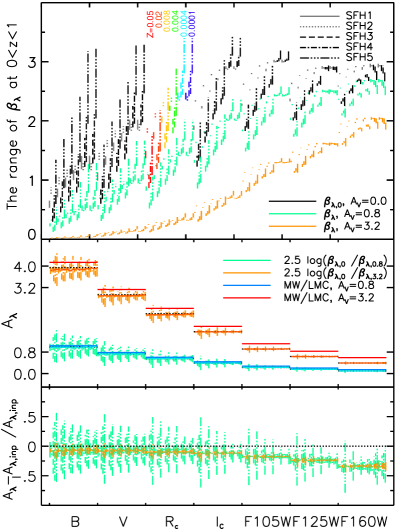
Figure 11: (top) The $\pm$1 $\sigma$ ranges of $\beta_{\lambda}$ values, referenced to $L$, for CSPs at 0 $<$ $z$ $<$ 1 for different choices of the optical–near-IR filters (bottom axis) for various metallicities, SFHs, and dust extinction values. (middle) Comparison between dust extinction values calculated using the ratio of $\beta_{\lambda,0}$ and $\beta_{\lambda}$ values (center values are connected), and dust extinction values, $A_{\lambda,\mathrm{inp}}$, using the MW/LMC extinction law (red and blue horizontal lines). Dotted black lines indicate $A_{\lambda,\mathrm{inp}}$ values with $-$0.05 and $-$0.19 mag offsets for $A_{V}$ = 0.8 and $A_{V}$ = 3.2, respectively (see text), which arise from neglecting the residual extinction in the $L$ filter. (bottom) Normalized ranges of recovered $A_{\lambda}$ with respect to $A_{\lambda,\mathrm{inp}}$. For high extinction values (orange), the $\beta_{\lambda}$ method can recover $A_{\lambda,\mathrm{inp}}$ to better than $\sim$20% for individual resolved galaxies when the redshift is only minimally constrained and when allowing a wide range in SFHs and metallicity. For large samples of galaxies, the $\beta_{V}$ method recovers the mean extinction to better than 10%.

In the middle panel of Figure 11, we compare the range of extinction values, $A_{\lambda}$, recovered from the $\beta_{\lambda}$ method:

$$A_{\lambda}=2.5\log{(\beta_{\lambda,0}/\beta_{\lambda})}\ ,$$ (5)

to the extinction values $A_{\lambda,\mathrm{inp}}$ imposed as

$$F_{\lambda,\mathrm{ext}}=F_{\lambda,\mathrm{int}}\cdot 10^{-0.4\cdot A_{\lambda,\mathrm{inp}}}$$ (6)

where $F_{\lambda,\mathrm{int}}$ and $F_{\lambda,\mathrm{ext}}$ are intrinsic and attenuated fluxes in each bandpass. These input extinction values are indicated by the horizontal red ($A_{V}$ = 3.2 mag) and blue ($A_{V}$ = 0.8 mag) lines. There are small systematic offsets of the median recovered $A_{\lambda}$ (indicated by the dark orange and cyan horizontal lines) from the $A_{\lambda,\mathrm{inp}}$ values (red and blue horizontal lines). In $V$, these offsets are $-$0.05 and $-$0.24 mag for $A_{V}$ = 0.8 and $A_{V}$ = 3.2 mag, respectively, of which $-$0.05 and $-$0.19 mag results from the assumption of the $\beta_{\lambda}$ method that the extinction in the $L$ band is negligible. The relative error due to this assumption becomes more obvious in the near-IR, where the extinction values are also small. In fact, in the near-IR filters, this can account for the full offset observed. The additional $\sim$0.05 mag offset observed for $A_{V}$ = 3.2 mag originates from the non-normal distribution of $A_{\lambda}$ values (we plot the center value of the range, not the mid-point).

In order to determine whether the near-IR filters are a better choice for the $\beta_{\lambda}$ technique over the optical filters, we compare their normalized scatter of $A_{\lambda}$ values in the bottom panel of Figure 11. After normalization, the level of scatter is consistent from the optical through the near-IR filters, but the assumption of negligible extinction in $L$ leads to a progressively worse underestimation of $A_{\lambda}$ in a relative sense. To have a sufficient handle on the extinction over a wide range of extinction values, it is therefore recommended to use the bluest filter available. From this panel we also see that the minimum scatter in the recovered $A_{\lambda}$ values consistently occurs for the lowest metallicity values and for SFHs characterized by little recent star formation (e.g., SFH3).

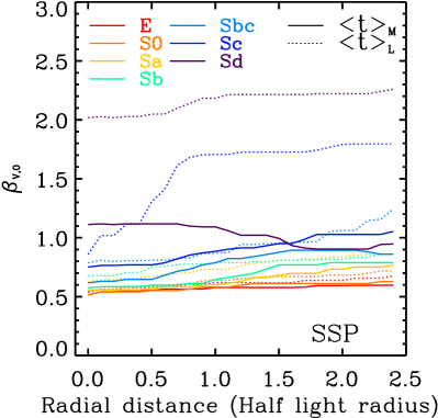
(a)    (b)

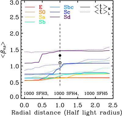
Figure 12: $\beta_{V\!,0}$ as a function of radius for galaxies of different Hubble type. (a) $\beta_{V\!,0}$ profiles derived from an array of SSP SEDs, and (b) mean $\langle$$\beta_{V\!,0}$$\rangle$ profiles resulting from 3000 arrays of stochastic SFH SEDs that we randomly generated using mass- (solid) and light-weighted (dotted) age and mass-weighted metallicity values from González Delgado et al. (2015; GD15). The solid (open) black circle indicates the value adopted by T09 for younger (older) stellar populations within NGC 959 (Sdm). For both SSP and stochastic SFH SEDs, we plot boxcar-smoothed radial profiles of $\beta_{V\!,0}$ and of average $\beta_{V\!,0}$ values, respectively (see text). The $\beta_{V\!,0}$ values vary little with radius for early-type galaxies for both SSPs and stochastic SFHs. For late-type galaxies, the presence of a bulge or older population would reduce the $\beta_{V\!,0}$ values within $R_{e}$.

3.3 $\beta_{\lambda,0}$ for Galaxies of Different Hubble Type at $z$ $\simeq$ 0

Nearby galaxies have been characterized by their morphologies and studied separately ever since Hubble (1926) first classified them based on their morphologies (e.g., de Vaucouleurs 1959; Odewahn 1995; van den Bergh 1998; Buta et al. 2007). Morphology can be estimated from single-band imaging data, and is known to closely correlate with both structural properties of galaxies and their SFHs (e.g., Humason et al. 1956; de Jong 1996; Jansen et al. 2000ab; Windhorst et al. 2002; Conselice et al. 2004; Taylor et al. 2005; Taylor-Mager et al. 2007; Hoyos et al. 2016). Examining the relation between $\beta_{\lambda,0}$ values and the morphology of galaxies will therefore be useful.

To address this, we first generate multiple arrays of SEDs with different SFH criteria: 1000 SFH3-ETG, 1000 SFH4-Spiral, and 1000 SFH5-LTG (see §2.2). GD15 presented integral field spectroscopy of 300 nearby galaxies of various Hubble types, and derived radial profiles of stellar population properties such as age, metallicity, and $A_{V}$. We adopt the mean of their weighted age and metallicity values for different Hubble types as a function of galactic radii. For spiral galaxies, we adopted the results of their face-on sample rather than edge-on sample, to minimize the effect of overlapping stellar populations and high mid-plane extinction. We then derive $\beta_{V\!,0}$ profiles for different Hubble types by comparing age and metallicity values of GD15 and our SEDs.

Table 5: $\beta_{V\!,0}$ values at the half-light radii, $\mathrm{R}_{e}$, of galaxies of different Hubble type, assuming either SSPs or CSPs with stochastic SFHs. The indicated ranges of $\beta_{V\!,0}$ for each model are derived from the uncertainties in the $\langle t\rangle_{\mathrm{L}}$, $\langle t\rangle_{\mathrm{M}}$, and $\langle Z\rangle_{\mathrm{M}}$ values. For each type of SFH, we compare mass- and luminosity-weighted $\beta_{V\!,0}$ values and ranges.

Hubble	SSP		Stochastic SFHs
Type	$\langle t\rangle_{\mathrm{L}}$	$\langle t\rangle_{\mathrm{M}}$	$\langle t\rangle_{\mathrm{L}}$	$\langle t\rangle_{\mathrm{M}}$	Family
E0	0.60${}^{+0.16}_{-0.14}$	0.57${}^{+0.14}_{-0.13}$	0.64${}^{+0.04}_{-0.07}$	0.65${}^{+0.03}_{-0.07}$	SFH3
S0	0.63${}^{+0.14}_{-0.13}$	0.58${}^{+0.12}_{-0.11}$	0.64${}^{+0.03}_{-0.07}$	0.64${}^{+0.03}_{-0.07}$	SFH3
Sa	0.74${}^{+0.17}_{-0.17}$	0.61${}^{+0.17}_{-0.16}$	0.74${}^{+0.14}_{-0.11}$	0.65${}^{+0.14}_{-0.03}$	SFH4
Sb	0.79${}^{+0.08}_{-0.09}$	0.65${}^{+0.11}_{-0.10}$	0.76${}^{+0.05}_{-0.03}$	0.72${}^{+0.06}_{-0.09}$	SFH4
Sbc	0.93${}^{+0.50}_{-0.13}$	0.78${}^{+0.17}_{-0.17}$	1.02${}^{+0.29}_{-0.27}$	0.77${}^{+0.26}_{-0.12}$	SFH4
Sc	1.65${}^{+0.49}_{-0.71}$	0.88${}^{+0.22}_{-0.18}$	1.09${}^{+0.37}_{-0.31}$	1.06${}^{+0.30}_{-0.31}$	SFH5
Sd	2.17${}^{+0.38}_{-0.62}$	1.03${}^{+0.30}_{-0.17}$	1.43${}^{+0.44}_{-0.36}$	1.39${}^{+0.43}_{-0.34}$	SFH5

At each discrete Age step in Table 6 for cosmic times later than 545 Myr ($z$ $<$ 9; see Figure 3), we calculated mass-weighted ages, $\langle t\rangle$_M, light-weighted ages, $\langle t\rangle$_L, and mass-weighted metallicities, $\langle Z\rangle$_M, for consistency with GD15 as

$$\langle t\rangle_{\mathrm{L}} = {\sum_{t^{\prime}=t_{0}}^{t}\log t^{\prime}\mathcal{F}(t^{\prime})\psi(t^{\prime})\delta t^{\prime}}\Big{/}{\sum_{t^{\prime}=t_{0}}^{t}\mathcal{F}(t^{\prime})\,\psi(t^{\prime})\,\delta t^{\prime}},\quad\$$ (7)

$$\langle t\rangle_{\mathrm{M}} = {\sum_{t^{\prime}=t_{0}}^{t}\log t^{\prime}\,\psi(t^{\prime})\,\delta t^{\prime}}\Big{/}{\sum_{t^{\prime}=t_{0}}^{t}\psi(t^{\prime})\,\delta t^{\prime}},$$ (8)

$$\langle Z\rangle_{\mathrm{M}} = {\sum_{t^{\prime}=t_{0}}^{t}\log Z(t^{\prime},Z_{0})\,\psi(t^{\prime})\,\delta t^{\prime}}\Big{/}{\sum_{t^{\prime}=t_{0}}^{t}\,\psi(t^{\prime})\,\delta t^{\prime}}$$ (9)

where $\mathcal{F}$ is the flux at 5635 Å, and $\psi(t)$ denotes the SFR, $Z_{0}$ is the metallicity at $z$ = 0, and metallicity is a function of cosmic time and $Z_{0}$, i.e., $Z(t^{\prime},Z_{0})$.

Figures 12(a) and (b) show smoothed median radial profiles of $\beta_{V\!,0}$ for galaxies modeled by SSP and stochastic SFHs, respectively, for different Hubble types. For stochastic SFHs, we used the SEDs of SFH3-ETG for E and S0, SFH4-Spiral for Sa–Sbc and SFH5-LTG for Sc and Sd Hubble types, respectively. $\langle$$\beta_{V\!,0}$$\rangle$ in Figure 12(b) is the average $\beta_{V}$ of 1000 randomly generated SFHs for each stochastic SFH family. In both panels, each profile was boxcar smoothed using a radial filter with a width corresponding to one half-light radius. Galaxies of E and S0 type have an almost constant $\beta_{V\!,0}$ value with increasing galactic radius for both SSPs and stochastic SFHs. Later types have higher and more fluctuating $\beta_{V\!,0}$ values and show a stronger dependence on radius. Table 5 lists representative mass- and light-weighted $\beta_{V\!,0}$ values at the half-light radii ($\mathrm{R}_{e}$) for each Hubble type for both SSPs and CSPs resulting from stochastic SFHs. We derive uncertainties in the $\beta_{V\!,0}$ values from the 1 $\sigma$ ranges presented in GD15 (their Figures 8, 13, and 18) by randomly varying the age and metallicity values in our models within these allowed ranges. The total range of luminosity-weighted $\beta_{V\!,0}$ values for nearby galaxies thus derived is 0.57–1.87 (the $\langle t\rangle_{\mathrm{L}}$ column for stochastic SFHs). For a galaxy of known morphological type, however, the likely range in $\beta_{V\!,0}$ is only $\sim$$\pm$10% with respect to the mean value for E, S0, Sa, and Sb galaxies, although late-type spiral and Magellanic-type galaxies display a wider $\pm$30–50% range. Figure 12(b) also shows that the mean $\beta_{V\!,0}$ values beyond $\mathrm{R}_{e}$ in the case of (observed) light-weighted ages are similar, but systematically higher (by up to $\sim$8–20% at 2.5 $\mathrm{R}_{e}$) than the (intrinsic) mass-weighted ages.

4 Discussion

We have generalized the $\beta_{V}$ method to a $\beta_{\lambda}$ method by placing the method on a more robust footing that does not require manual estimation of the intrinsic flux ratios from pixel histograms and that provides evaluation of the associated uncertainties for a large number of optical–near-IR and mid-IR filters. Stars with young ages and low metallicities emit light with SEDs that have high $\beta_{\lambda,0}$ values, and as stars age and as stars become more metal-rich, the $\beta_{\lambda,0}$ values decrease and stabilize. T09 also observed this trend in their 2D map of $\beta_{V\!,0}$ values (their Figure 2), which was based on SSPs and the model SEDs from Anders & Fritze-von Alvensleben (2003).

4.1 Application to Discrete Sets of Filters at 0 $<$ $z$ $<$ 1.9

While using near-IR filters results in a narrower $\beta_{\lambda,0}$ range over the redshift range 0 $<$ $z$ $<$ 1 (see Figure 11), after normalization, the relative dispersion in the simulated $A_{\lambda}$ values is comparable in the optical and near-IR filters. One should be cautious about using near-IR bandpasses at low redshift, however, since the offset due to the residual extinction in the mid-IR reference filter becomes more noticeable (see Figure 11, bottom panel). Nonetheless, HST/WFC3 near-IR filters may be used to sample visible rest-frame wavelengths up to $z$ $\sim$ 1.9. In that case, one should use the filter nearest the corresponding rest-frame wavelength when applying the $\beta_{\lambda}$ method. For instance, at $z$ $\simeq$ 1.9, the HST/WFC3 IR F160W filter would sample rest-frame $V$, and the JWST/MIRI F1000W bandpass would sample rest-frame 3.5 µm, so one can use the $\beta_{V\!,0}$ values presented in this paper and on our website.

Although the value of $\beta_{V\!,0}$ will depend on the detailed shape of the throughput curves of the filters sampling the rest-frame $V$ and 3.5 µm light, Figs. 7 and 8 show that such dependence for even quite mismatched filters (e.g., $L^{\prime}$ and WISE $W$1) affects $\beta_{V\!,0}$ at the $\lesssim$20% level. For bandpasses that are better matched to the $L$ band, such as Spitzer/IRAC $I$1 and JWST/NIRCam F356W, the differences tend to be at the $\lesssim$5% level, except for very young ($<$ 10 Myr) stellar ages and for high metallicities ($Z$ $>$ 0.02). A similar caution applies at redshifts where the bandpass sampling rest-frame $V$ light differs very much from that of the $V$ filter at $z$ $\sim$ 0. Nonetheless, the dependence of the accuracy of the $\beta_{\lambda}$ technique on the choice of filters in both the optical–near-IR and mid-IR is weak.

4.2 Application to Galaxy Samples Using Realistic SFHs

We have extended our models from SSP to more complex SFHs. In real galaxies, the observed $\beta_{\lambda}$ flux ratios are also affected by spatial resolution, as light from a broad region within a galaxy would result from a combination of various stellar populations, each resulting from different complex stochastic SFHs. For example, Galliano et al. (2011) obtained a $\sim$50% difference in inferred dust mass when they used integrated SEDs with different spatial resolutions. The sharp features in a map of $\beta_{\lambda,0}$ values of SSPs in Figure 6 at young ($\lesssim$100 Myr) ages are smeared out when a galaxy has a more complex SFH, such as an exponentially declining SFH. In addition, we adopt five families of stochastic SFHs that are composed of multiple exponentially declining star formation episodes, and probe variations of $\beta_{\lambda,0}$ values over cosmic history. For a minimally constrained redshift range, 0 $<$ $z$ $<$ 1, the variation in $\beta_{\lambda}$ is dominated by SFH5, representing late-type galaxies. The other SFH families show more modest variations for a given metallicity and choice of optical–near-IR filter (see Figs. 10 and 11). Metallicity evolution is taken into account and makes a noticeable difference (Figs. 9 and 10(b)), predicting higher $\beta_{\lambda,0}$ values than in the no-evolution case, especially at higher redshifts and for the higher-metallicity stellar populations at those redshifts.

We first consider the applicability of the $\beta_{\lambda}$ method for a galaxy sample with a large effectively unconstrained redshift range (0 $\lesssim$ $z$ $\lesssim$ 4). The $\beta_{V\!,0}$ values could span 0.6–4.7 in that case (see Figure 10 and §3.2). For the minimally constrained 0 $<$ z $<$ 1 redshift range, the scatter in recovered $A_{\lambda}$ is $\sim$0.2 mag in $V$ and decreases with increasing wavelength, but varies little with the amount of input extinction imposed (Figure 11, middle panel). The normalized difference of the recovered and input extinction, $(A_{\lambda}-A_{\lambda,\mathrm{inp}})/A_{\lambda,\mathrm{inp}}$, on the other hand, is $\sim$23% and $\sim$16% for $A_{V}$ = 0.8 and $A_{V}$ = 3.2 mag, respectively (see bottom panel of Fig 11). Note, however, that this reflects what one would expect for individual galaxies (or regions therein). The mean difference of the recovered and input extinction values is close to 0.0, suggesting that the $\beta_{\lambda}$ method can accurately recover the mean extinction for a larger sample of galaxies spanning a range of redshifts, SFHs, and metallicities, and also of a population of galaxies of a given type within a narrow redshift range. The highly attenuated case ($A_{V}$ = 3.2) has a smaller scatter, because the extinction dominates the shape of the SED more than any other factors, like stellar age or metallicity. For normal ($A_{V}$ $\lesssim$ 1) galaxies, we recommend using extra information, such as galaxy size and magnitudes, or if available, a photometric redshift estimate (or a spectroscopic redshift), for selecting the corresponding $\beta_{\lambda,0}$ value.

4.3 Dependence of $\beta_{\lambda,0}$ on Hubble Type and Weighting

Because one can classify the morphology of a galaxy with a single-band image (with the caveat of a slight rest-frame wavelength dependence of the morphology for different Hubble types, as found by Windhorst et al. 2002), studying the relation between galactic morphology and $\beta_{\lambda,0}$ values can be useful, since the $\beta_{\lambda}$ method is specifically designed as a dust-correction technique when a very limited number of filters are available. We used the SFH3–5 criteria (see §2.2) to generate multiple arrays of SEDs combined with the stellar population parameters from GD15 to obtain the $\beta_{V\!,0}$ values for different Hubble types (see Figure 12(b)). For a given galaxy type, $\beta_{V\!,0}$ values vary little as a function of galactic radius. Later Hubble types typically have higher $\beta_{V\!,0}$ values (see also Table. 5), as their stellar populations tend to be younger and metallicities lower than earlier types (see Figure 17 in GD15). We also investigate the effect of different weighting methods. The ratios between $\beta_{V\!,0}$ values resulting from using mass- and light-weighted ages are shown in Figure 13 as a function of Hubble type. We find no strong dependence of the median ratios of $\beta_{V\!,0}$ values with different weighting methods on Hubble type. Also indicated in Figure 13 are the quartile ranges and the $\pm$3 $\sigma$ range of these ratios. Light-weighted $\beta_{V\!,0}$ values are unlikely to differ by more than 10% (30%) from mass-weighted ones for early-type (late-type) galaxies.

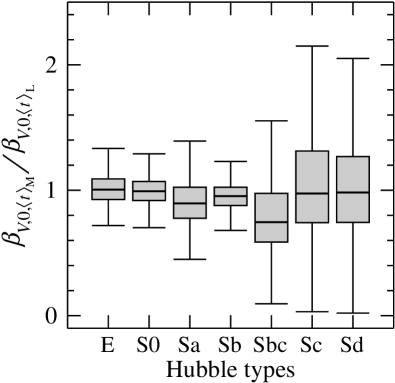
Figure 13: Ratio of $\beta_{V\!,0}$ values for mass- and light-weighted ages for different Hubble types. For each Hubble type, we randomly generated 1000 $\beta_{V\!,0}$ values each for both mass- and light-weighted ages, adopting the mean and 1 $\sigma$ values at $R_{e}$ listed in Table 5. The horizontal lines inside the boxes represent the median ratios. The gray boxes indicate the quartile range, while the error bars contain 99.7% of the distribution. The weighting method does not affect the inferred $\beta_{V\!,0}$ value for a given Hubble type in a systematic manner.

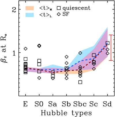
Figure 14: $\beta_{V}$ values at the half-light radii, $R_{e}$, as a function of Hubble type (dashed lines) using mass- (dark brown), or light-weighted (blue) ages and $A_{V}$ values. The shaded regions are the $\pm$1 $\sigma$ ranges of $\beta_{V}$ values. We overplot the $\beta_{V}$ values of nearby galaxies from Brown et al. (2014). The dashed curves represent median trends. The red error bar indicates the range of $\beta_{V}$ values observed by T09 in NGC 959 (Sdm).

To test the reliability of the $\beta_{\lambda}$ method, in Figure 14 we compare the inferred $\beta_{V}$ values with observed $\beta_{V}$ values for nearby galaxies. We used $\langle$$\beta_{V\!,0}$$\rangle$ values from Figure 12(b) at the half-light radius and the allowed 1 $\sigma$ range therein computed by varying ages and metallicities within the 1 $\sigma$ observed ranges of GD15 (see their Figs. 8, 11, and 18), coupled with the mean $A_{V}$ values of the corresponding Hubble types at the half-light radii from GD15 ($\langle$$A_{V}$$\rangle$=0.01, 0.06, 0.22, 0.25, 0.27, 0.26, and 0.18 for E, S0, Sa, Sb, Sbc, Sc, and Sd galaxies) to derive the predicted ranges for the $\beta_{V}$ values one would observe for each of the Hubble types. The dark brown (blue) dashed line and the orange (blue) shaded region indicate the median and 1 $\sigma$ range of the $\beta_{V}$ values when using mass- (light-) weighted ages, and the violet region represents the region of overlap. The $\beta_{V}$ values of 23 nearby ($z$ $\lesssim$ 0.05) quiescent (limited star formation) and 28 normally star-forming galaxies from Brown et al. (2014) are overplotted. Galaxies with “peculiar” morphologies, and galaxies with “SF/AGN”, or “AGN” BPT classes are excluded. Brown et al. (2014) combined multiple spectra and broadband data of nearby galaxies, and carefully performed aperture corrections in order to construct a template library. We used their aperture-corrected SDSS $g$, $r$ band and the Spitzer/IRAC Channel 1 ($I$1) magnitudes to derive the $\beta_{V}$ values. The SDSS $g$ and $r$ band magnitudes are converted into $V$-band magnitudes using the transformation equation from Jester et al. (2005). We take the Spitzer $I$1 magnitudes as proxy for $L$-band magnitudes, since Figure 7 and 8 show that the resulting $\beta_{V\!,0}$ are at most $\lesssim$10% higher and show little structure. Our model and observation agree well, except in a few cases for star forming galaxies with Hubble type E and S0, which seem to be outliers (see § 2.1.4 of Brown et al. 2014). Last, we note that the 0.82–1.41 range of $\beta_{V}$ values observed by T09 for Sdm galaxy NGC 959 is in good agreement with the trend in values inferred for the galaxy sample of Brown et al. (2014), as well as with the range predicted by our models in Figure 14, and that their empirical values adopted for the intrinsic $\beta_{V\!,0}$ ratios are consistent with those predicted in the present study (e.g., Figure 12(b) and Table 5 (Sd)). We conclude that our model $\beta_{\lambda,0}$ values agree with the observations for at least nearby ($z$ $\simeq$ $0$) galaxies.

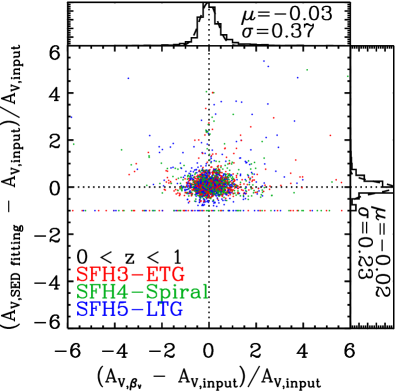
(a)      (b)

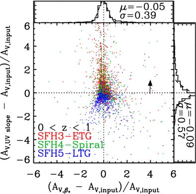
Figure 15: Comparison of the $\beta_{V}$ method to other dust-correction methods. (a) Comparison of the normalized difference between recovered and input extinction values in $V$ for both the SED-fitting and $\beta_{V}$ methods. The $\beta_{V}$ method shows a comparable average offset and scatter around the true value of $A_{V}$ to the SED-fitting method, although it requires less information. To derive $A_{V}$ for our families of stochastic SFHs, we used the 0 $<$ $z$ $<$ 1 average values of $\beta_{V\!,0}$ of 1.40, 1.48, and 1.78 for SFH3, SFH4, and SFH5, respectively. (b) As (a) for both the UV-slope and $\beta_{V}$ methods. The $A_{V}$ values recovered by the UV-slope method are systematically slightly lower than the $A_{V,\mathrm{inp}}$ values ($\mu$ = $-$0.10 mag; for a MW/LMC extinction law as in Calzetti et al.1994), and the scatter is larger than for the $\beta_{V}$ method ($\sigma$ = 0.60 vs. 0.38 mag). The black arrow shows how the offset would change if we adopted a Calzetti et al. (2000) extinction law ($\mu$ = $+$1.10).

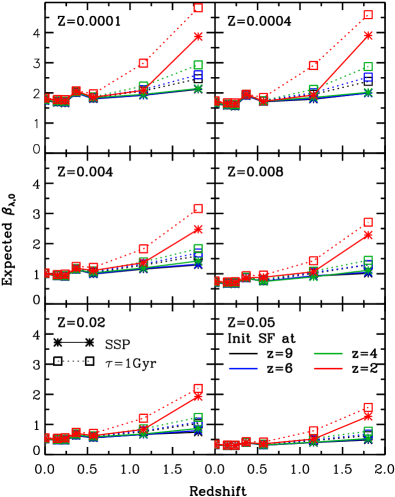
(a)      (b)

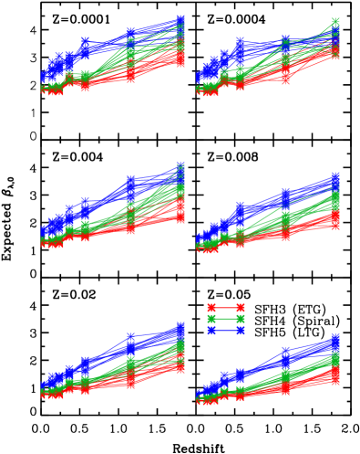
Figure 16: Expected intrinsic flux ratios $\beta_{\lambda,0}$ as a function of redshift for six metallicities and various SFHs, for redshifts where well-matched pairs of optical or near-IR HST and mid-IR JWST filters correspond to rest-frame $V$ and 3.5 µm, respectively. (a) $\beta_{\lambda,0}$ for SSPs (solid) and exponentially declining SFHs with an $e$-folding time of 1 Gyr. Tracks are color-coded (as indicated in the lower right panel) according to the redshift of onset of the instantaneous (SSP) or extended star formation. At a fixed metallicity value and starburst onsets well before $z$ = 2, $\beta_{\lambda,0}$ remains nearly constant over the entire 0 $\leq$ $z$ $\leq$ 2 redshift range. (b) The same as (a) for 10 examples of each of our three stochastic SFH families. Except for the two very lowest metallicities, $\beta_{\lambda,0}$ increases with redshift in a nearly linear fashion, with little overlap between the tracks for the three SFH families.

4.4 Comparison with Other Methods

We next compare the $\beta_{V}$ method to other established methods of correcting galaxy SEDs for attenuation by cosmic dust. In Figure 15(a), we compare the relative differences between recovered and input extinction values (normalized to the input value, $A_{V,\mathrm{inp}}$) for (multiband) SED fitting and the $\beta_{V}$ method. When we impose minimal constraints on the allowed redshift range (0 $<$ $z$ $<$ 1), the SED-fitting method provides estimates that are closer to the true input value, $A_{V,\mathrm{inp}}$, on average ($\mu$ = $-$0.02 vs. $-$0.03 mag), and with a smaller scatter ($\sigma$ = 0.23 vs. 0.37 mag). The small fraction of data points for the SED-fitting method at a normalized difference of exactly $-$1 result where the best fit was for $A_{V}$ = 0 mag (out of the finite set of discrete extinction values), when any non-zero extinction was imposed. These data points do not significantly broaden the distribution. The $\beta_{V}$ method shows a somewhat larger scatter, but not by much, considering that the $\beta_{V}$ method requires significantly less information than the SED-fitting method to correct for dust extinction. In order to make this comparison, we construct a large set of randomly generated SEDs for stochastic SFHs representing early-type, spiral, and late-type galaxies (our SFH families SFH3, SFH4, and SFH5; see § 2.2), sampled at random redshifts in the range 0 $<$ $z$ $<$ 1, and with random amounts of extinction (0 $\leq$ $A_{V}$ $\leq$ 2 mag) applied and characterized by a randomly selected extinction law (Milky Way/Large Magellanic Cloud; MW/LMC, SMC, or Calzetti). To apply the $\beta_{V}$ method and recover $A_{V}$, we assume that the appropriate SFH family to use would be known a priori from the morphological type of an observed galaxy, and only minimally restrict the redshift to the same 0 $<$ $z$ $<$ 1 range. The average values of $\beta_{V\!,0}$ in this redshift range are 1.40, 1.48, and 1.78 for SFH3, SFH4, and SFH5, respectively. Using Eq. 5, we then infer (recover) for each model SED an extinction value $A_{V}$ from the appropriate mean $\beta_{V\!,0}$ value and the observed ($V$ $-$ $L$) color (expressed as a flux ratio, i.e., $\beta_{V}$). As templates for the SED-fitting method, we used the same set of 724 unique and distinguishable SSP SEDs (see Appendix A), either used as is, or incorporated into CSP SEDs for seven exponentially declining SFHs, or into our suite of stochastic SFHs (§ 2.2) with 300 random realizations for each of the SFH3, SFH4, and SFH5 families. The comparison should therefore not be biased by differences in the adopted set of input galaxy SED templates. Using the full rest-frame 0.4 $\leq$ $\lambda$ $\leq$ 3.75 µm portion of each of the SEDs, we perform the SED fit to characterize both stellar population parameters and recover $A_{V}$. This represents a best-case scenario, the results of which are shown in Figure 15(a). If, as would be the case for a more realistic galaxy survey, the SED is sampled through multiple filters, each resulting in a single flux density data point, the comparison is unlikely to be more favorable for the SED-fitting method, although the allowed redshift range may be narrowed for galaxies displaying a strong 4000 Å break.

In Figure 15(b) we compare the relative differences between recovered and input extinction values for the UV continuum slope method and the $\beta_{V}$ method. Calzetti et al. (1994) studied the effect of dust extinction on the UV continuum in spectra of local starburst galaxies, and provided a relation between the UV power-law index $\beta$ and the optical depth $\tau$ (their Eq. 4). For a best-case scenario, we use their fitting windows, sampling the 1268–2580 Å wavelength range while excluding the interval that might be affected by a 2175 Å-bump (if present), and adopt a MW/LMC extinction law to match Calzetti et al. (1994). The $\beta_{V}$ method underestimates the extinction values in this test by $\sim$5% (compared to 9% for the UV continuum slope method) and shows a smaller scatter than the UV-slope method: $\sigma$ = 0.39 mag for the $\beta_{V}$ method versus 0.57 mag for the UV-slope method. Note, however, that if we were to adopt a Calzetti et al. (2000) extinction law instead, this would result in recovered extinction values for the UV-slope method that are systematically higher than the input values by an amount indicated by the black arrow in Figure 15(b), whereas the mean difference $\mu$ would change by only $+$0.04 for the $\beta_{V}$ method. We also note that the UV-slope method shows a stronger dependence of the recovered $A_{\lambda}$ on SFH (galaxy type) than does the $\beta_{V}$ method.

Our tests therefore show that the $\beta_{V}$ method can indeed be used to infer $A_{V}$ and correct for dust extinction to a level of fidelity that is comparable to that of more established methods, with fewer or more readily obtainable data. In particular, we note that systematic offsets in the recovered extinction values are no worse than for these two commonly used methods. These properties makes the $\beta_{V}$ ($\beta_{\lambda}$) method a prime candidate for application to large imaging surveys with JWST of fields already observed with HST in the visible–near-IR.

4.5 $\beta_{\lambda,0}$ for Galaxies Observed with HST and JWST

For a $z$ $\simeq$ 0.3 galaxy, rest-frame optical images from HST/ACS WFC or WFC3 UVIS (F606W, …, F850LP) and rest-frame $\sim$3.5 µm mid-IR images from JWST/NIRCam (F410M, F444W, F480M) will have resolutions of $\sim$0$\farcs$06–0$\farcs$09 and $\lesssim$0$\farcs$19, resolving regions of $\lesssim$875 pc in size. At $z$ $\sim$ 2, HST/WFC3 IR F160W and JWST/MIRI F1000W sample rest-frame $V$ and 3.5 µm, but the resulting resolution of $\sim$0$\farcs$48 would not allow resolving regions smaller than $\sim$4 kpc. The combination of these two space telescopes will make studies of galaxies over billions of years possible in unprecedented detail. Specifically for this purpose, we therefore generate model SEDs and calculate $\beta_{\lambda,0}$ values for a set of discrete redshifts at which well-matched HST and JWST filter pairs sample rest-frame $V$ and 3.5 µm emission. At redshifts $z$ = 0, 0.14, 0.24, and 0.37, well-matched HST and JWST/NIRCam filter pairs are (F555W, F356W), (F606W, F410M), (F625W, F444W), and (F775W, F480M), respectively. At $z$ = 0.57, 1.16, and 1.8, suitable HST and JWST/MIRI filter pairs are (F814W, F560W), (F110W, F770W), and (F160W, F1000W). In Figure 16(a) we show the resulting tracks of $\beta_{\lambda,0}$ versus redshift for six different metallicities and both SSP and exponentially declining SFHs with an $e$-folding time of 1 Gyr, and do so for four different redshifts of onset of either the instantaneous or extended star formation. For SF onset times well before $z$ $\sim$ 2, the tracks remain nearly constant over the entire redshift range at a given metallicity, although the mean $\beta_{\lambda,0}$ values decrease systematically with increasing metallicity ($\langle$$\beta_{\lambda}$$\rangle$_z<1.2 $\simeq$ 1.9, 1.8, 1.0, 0.8, 0.5, and 0.4 for $Z$ = 0.0001, 0.0004, 0.004, 0.008, 0.02, and 0.05, respectively). We similarly derive $\beta_{\lambda,0}$ for these HST and JWST filter pairs for our three families of stochastic SFHs. In Figure 16(b) we show $\beta_{\lambda,0}$ versus redshift for the same six metallicity values for 10 examples of each SFH family. The $\beta_{\lambda,0}$ tracks for each SFH family increase systematically and almost linearly with increasing redshift. The slopes of those tracks differ for each family, SFH5 (late-type) having the steepest slope and SFH3 (early-type) having the shallowest. Only at the two lowest metallicities do the late-type tracks start to deviate from their linear increase with redshift to overlap the tracks of spiral (at $z$ $>$ 1) and even early-type galaxies (for $z$ $\gtrsim$ 1.5). For higher metallicities there appears to be little overlap between the tracks for the three SFH families. With some constraints on the stellar metallicity, SFH, and redshift, the $\beta_{\lambda}$ method can be a powerful tool to correct the spatially resolved images for large samples of galaxies observed with HST and JWST at moderate redshifts for the effects of extinction by dust.

5 Summary

We combined SSP SEDs from the Starburst99 and BC03 codes for young and old stellar ages, respectively, and generated arrays of CSP SEDs for a large variety of exponentially declining and stochastic SFHs by stacking SSP SEDs as a function of the adopted time-dependent SFRs. For our large suite of models with stochastic SFHs, we take the average metallicity evolution as a function of cosmic age into account. We calculated the intrinsic flux ratios $\beta_{\lambda,0}$ between rest-frame visible–near-IR and rest-frame mid-IR 3.5 µm on a grid of six metallicities and 16 ages of stellar populations for 13 different SFH families, for 29 visible–near-IR filters, and 5 mid-IR filters with central wavelengths near 3.5 µm. We find that taking metallicity evolution into account results in significantly higher $\beta_{\lambda,0}$ values at higher redshifts and for higher-metallicity stellar populations at those redshifts. We also provide the range of $\beta_{V\!,0}$ and $\beta_{V}$ for different Hubble types of nearby galaxies, and confirm that our models agree with the observed $\beta_{V}$ values. We demonstrated that the $\beta_{V}$ method can infer $A_{V}$ to a level of fidelity that is comparable to that of more established methods. We conclude that the $\beta_{V}$ method and its extension, the $\beta_{\lambda}$ method presented here, are valid as a first-order dust-correction method, when using the morphology and size of a galaxy as broad a priori constraints to its SFH and redshift, respectively. The $\beta_{\lambda}$ method will be applicable to large samples of galaxies for which resolved imagery is available in one rest-frame visible–near-IR filter and one rest-frame $\lambda$ $\sim$ 3.5 µm bandpass. We make our CSP synthesis models and all our results available via a dedicated website in the form of FITS and PNG maps, and ASCII data tables of $\beta_{\lambda,0}$ values as a function of age and metallicity.

6 References

Allamandola, L.J., Tielens, A.G.G.M., & Barker, J.R. 1989, ApJS, 71, 733

Anders, P., & Fritze-von Alvensleben, U. 2003, A&A 401, 1063

Avila, R., et al. 2015, “ACS Instrument Handbook”, Version 14.0 (Baltimore: STScI)

Behroozi, P.S., Wechsler, R.H., & Conroy, C. 2013, ApJ 770, 57

Bell, E.F., Gordon, K.D., Kennicutt, R.C. Jr., & Zaritsky, D. 2002, ApJ 565, 994

Bessell, M.S. 1979, PASP 91, 589

Bessell, M.S. 1990, PASP 102, 1181

Bessell, M.S. 2005, ARA&A, 43, 293

Bessell, M.S., & Brett, J.M. 1988, PASP 100, 1134

Boissier, S., Boselli, A., Buat, V., Donas, J., & Milliard, B. 2004, A&A 424, 465

Boselli, A., Gavazzi, G., & Sanvito, G. 2003, A&A 402, 37

Brown, M.J.I., Moustakas, J., Smith, J.-D.T., et al. 2014, ApJS 212, 18

Bruzual, G., & Charlot, S. 2003, MNRAS 344, 1000 (BC03)

Buat, V., & Xu, C. 1996, A&A 306, 61

Buat, V., Iglesias-Páramo, J., Seibert, M., et al. 2005, ApJ 619, L51

Buta, R.J., Corwin, H.G., & Odewahn, S. C. 2007, The de Vaucouleurs Altlas of Galaxies (Cambridge: Cambridge Univ. Press)

Calzetti, D., Kinney, A.L., & Storchi-Bergmann, T. 1994, ApJ 429, 582

Calzetti, D., Armus, L., Bohlin, R.C., et al. 2000, ApJ 533, 682

Calzetti, D., Kennicutt, R.C. Jr., Bianchi, L., et al. 2005, ApJ 633, 871

Caplan, J., & Deharveng, L. 1985, A&AS 62, 63

Caplan, J., & Deharveng, L. 1986, A&A 155, 297

Cerviño, M., & Mas-Hesse, J.M. 1994, A&A 284, 749

Chabrier, G. 2003, PASP 115, 763

Charbonnel, C., Meynet, G., Maeder, A., Schaller, G., & Schaerer, D. 1993, A&AS, 101, 415

Charlot, S., & Fall, S.M. 2000, ApJ 539, 718

Cohen, M., Wheaton, W.A., & Megeath, S.T. 2003, AJ 126, 1090

Colina, L., & Bohlin, R. C. 1994, AJ 108, 1931

Conselice, C.J., Grogin, N.A., Jogee, S., et al. 2004, ApJL 600, L139

Dale, D.A., Helou, G., Contursi, A., Silbermann, N.A., & Kolhatkar, S. 2001, ApJ 549, 215

da Silva, R.L., Fumagalli, M., & Krumholz, M. 2012, ApJ 745, 145

de Jong, R.S. 1996, A&A 313, 377

Deo, R.P., Crenshaw, D.M., & Kraemer, S.B. 2006, AJ 132, 321

de Vaucouleurs, G. 1959, Handbuch der Physik 53, 275

Dickinson, M., Giavalisco, M., & GOODS Team 2003, The Mass of Galaxies at Low and High Redshift, 324

Dressel, L., 2015. “Wide Field Camera 3 Instrument Handbook, Version 7.0” (Baltimore: STScI)

Driver, S.P., Popescu, C.C., Tuffs, R.J., et al. 2008, ApJ 678, L101

Duce, D.A., Adler, M., Boutell, T., et al. 2004, ISO/IEC 15948:2004 (http://www.libpng.org/pub/png/spec/iso/ and W3C REC-PNG-20031110 https://www.w3.org/TR/PNG/)

Elmegreen, D.M. 1980, ApJS 43, 37

Elsasser, W.M. 1938, ApJ 87, 497

Fazio, G.G., Hora, J.L., Allen, L.E., et al. 2004, ApJS 154, 10

Fioc, M., & Rocca-Volmerange, B. 1997, A&A 326, 950

Fitzpatrick, E.L. 1999, PASP 111, 63

Ford, H.C., Clampin, M., Hartig, G.F., et al. 2003, Proc. SPIE 4854, 81

Galliano, F., Hony, S., Bernard, J.-P., et al. 2011, A&A 536, A88

Gardner, J. P., Mather, J.C., Clampin, M., et al. 2006, Space Science Reviews, 123, 485

Gerola, H., & Seiden, P.E. 1978, ApJ 223, 129

Giavalisco, M., Ferguson, H. C., Koekemoer, A. M., et al. 2004, ApJL 600, L93

Girardi, L., Bressan, A., Bertelli, G., & Chiosi, C. 2000, A&AS 141, 371

González Delgado, R.M., García-Benito, R., Pérez, E., et al. 2015, A&A, 581, A103 (GD15)

Gordon, K.D., Clayton, G.C., Misselt, K.A., Landolt, A.U., & Wolff, M.J. 2003, ApJ 594, 279

Grogin, N.A., Kocevski, D.D., Faber, S.M., et al. 2011, ApJS 197, 35

Gunn, J.E., Carr, M., Rockosi, C., et al. 1998, AJ 116, 3040

Hanisch, R.J., Farris, A., Greisen, E.W., et al. 2001, A&A, 376, 359

Hayes, D. S., & Latham, D. W. 1975, ApJ 197, 593

Horner, S.D., & Rieke, M. J. 2004, SPIE 5487, 628

Hoyos, C., Aragón-Salamanca, A., Gray, M. E., et al. 2016, MNRAS 455, 295

Hubble, E.P. 1926, ApJ 64, 321

Humason, M.L., Mayall, N.U., & Sandage, A.R. 1956, AJ 61, 97

Jansen, R.A., Franx, M., Fabricant, D., & Caldwell, N. 2000a, ApJS 126, 271

Jansen, R.A., Fabricant, D., Franx, M., & Caldwell, N. 2000b, ApJS 126, 331

Jarret, T.H., Cohen, M., Masci, F., Wright, E., Stern, D., et al. 2011, ApJ 735, 112

Jester, S., Schneider, D.P., Richards, G.T., et al. 2005, AJ 130, 873

Kauffmann, G., Heckman, T.M., De Lucia, G., et al. 2006, MNRAS 367, 1394

Kelvin, L.S., Driver, S.P., Robotham, A.S.G., et al. 2014, MNRAS 444, 1647

Kennicutt, R.C. Jr., Hao, C.-N., Calzetti, D., et al. 2009, ApJ 703, 1672

Kessler, M.F., Steinz, J.A., Anderegg, M.E., et al. 1996, A&A 315, L27

Koekemoer, A.M., Faber, S.M., Ferguson, H.C., et al. 2011, ApJS 197, 36

Kong, X., Charlot, S., Brinchmann, J., & Fall, S.M. 2004, MNRAS 349, 769

Kroupa, P. 2002, Science 295, 82

Kurucz, R.L. 1993, CDROM No. 13, 18 (Cambridge MA: Smithsonial Astrophysical Observatory); http://kurucz.harvard.edu

Léger, A., & Puget, J. L. 1984, A&A, 137, L5

Leitherer, C., Schaerer, D., Goldader, J.D., et al. 1999, ApJS 123, 3 (Starburst99)

Lindblad, B. 1941, Stockholms Observatoriums Annaler 13, 8

Maíz-Apellániz, J., Pérez, E., & Mas-Hesse, J.M. 2004, AJ 128, 1196

Maiolino, R., Nagao, T., Grazian, A., et al. 2008, A&A 488, 463

Maraston, C. 2005, MNRAS 362, 799

Marigo, P., Girardi, L., Bressan, A., et al. 2008, A&A 482, 883

Mathis, J.S., Rumpl, W., & Nordsieck, K.H. 1977, ApJ 217, 425

Meurer, G.R., Heckman, T.M., & Calzetti, D. 1999, ApJ 521, 64

Schaerer, D., Charbonnel, C., Meynet, G., Maeder, A., & Schaller, G. 1993b, A&AS, 102, 339

Misselt, K.A., Clayton, G.C., & Gordon, K.D. 1999, ApJ 515, 128

Neugebauer, G., Habing, H.J., van Duinen, R., et al. 1984, ApJ 278, L1

Odewahn, S. C. 1995, ApL&C, 31, 55

Oke, J.B. 1974, ApJS 27, 21

Oke, J.B., & Gunn, J.E. 1983, ApJ 266, 713

Panuzzo, P., Bressan, A., Granato, G.L., Silva, L., & Danese, L. 2003, A&A 409, 99

Petersen, L., & Gammelgaard, P. 1997, A&A 323, 697

Pilbratt, G.L. 2004, Proc. SPIE 5487, 401

Planck Collaboration, Ade, P. A. R., Aghanim, N., et al. 2016, A&A 594, A13; “Planck 2015 Results. XIII. Cosmological Parameters”

Postman, M., Coe, D., Benítez, N., et al. 2012, ApJS 199, 25

Price, S.D., Carey, S.J., & Egan, M.P. 2002, Adv. Space Research 30, 2027

Relaño, M., Lisenfeld, U., Vilchez, J. M., & Battaner, E. 2006, A&A 452, 413

Rieke, M. 2011, in ASP Conf. Ser. 446, Galaxy Evolution: Infrared to Milimeter Wavelength Perspective, ed. W. Wang et al. (San Francisco, CA: ASP), 331

Roussel, H., Gil de Paz, A., Seibert, M., et al. 2005, ApJ 632, 227

Rudy, R.J. 1984, ApJ 284, 33

Salpeter, E.E. 1955, ApJ 121, 161

Scoville, N.Z., Polletta, M., Ewald, S., et al. 2001, AJ 122, 3017

Schaerer, D., Meynet, G., Maeder, A., & Schaller, G. 1993a, A&AS, 98, 523

Schaerer, D., Charbonnel, C., Meynet, G., Maeder, A., & Schaller, G. 1993b, A&AS, 102, 339

Schaller, G., Schaerer, D., Meynet, G., & Maeder, A. 1992, A&AS, 96, 269

Scoville, N., Abraham, R.G., Aussel, H., et al. 2007, ApJS 172, 38

Tamura, K., Jansen, R.A., & Windhorst, R.A. 2009, AJ 138, 1634 (T09)

Tamura, K., Jansen, R.A., Eskridge, P.B., Cohen, S.H., & Windhorst, R.A. 2010, AJ 139, 2557

Taylor, V.A., Jansen, R.A., Windhorst, R.A., Odewahn, S.C., & Hibbard, J.E. 2005, ApJ 630, 784

Taylor-Mager, V.A., Conselice, C.J., Windhorst, R.A., & Jansen, R.A. 2007, ApJ 659, 162

Trumpler, R.J. 1930, PASP 42, 214

van den Bergh, S. 1998, Galaxy Morphology and Classification (Cambridge: Cambridge Univ. Press)

Vazdekis, A., Sánchez-Blázquez, P., Falcón-Barroso, J., et al. 2010, MNRAS 404, 1639

Vázquez, G.A., & Leitherer, C. 2005, ApJ 621, 695

Viallefond, F., Goss, W.M., & Allen, R.J. 1982, A&A 115, 373

Walcher, J., Groves, B., Budavári, T., & Dale, D. 2011, Ap&SS, 331, 1

Walterbos, R.A.M., & Kennicutt, R.C. Jr. 1988, A&A 198, 61

Waller, W.H., Gurwell, M., & Tamura, M. 1992, AJ 104, 63

Wells, D.C., Greisen, E.W., & Harten, R.H. 1981, A&AS, 44, 363

Werner, M.W., Roellig, T.L., Low, F.J., et al. 2004, ApJS 154, 1

Windhorst, R.A., Taylor, V.A., Jansen, R.A., et al. 2002, ApJS 143, 113

Windhorst, R.A., Cohen, S.H., Hathi, N.P., et al. 2011, ApJS 193, 27

Witt, A.N., Thronson, H.A. Jr., & Capuano, J.M. Jr. 1992, ApJ 393, 611

Wright, E.L., Eisenhardt, P.R.M., Mainzer, A.K., et al. 2010, AJ 140, 1868

Xu, C., & Helou, G. 1996, ApJ 456, 152

Appendix A A SET OF DISTINGUISHABLE SSPs

We construct our combined model SSP SEDs for a manageably small, yet comprehensive set of parameters that span the range of representative stellar population properties and dust extinction. We consider six metallicity and 16 age values of the stellar population, four extinction laws, and eight $V$-band extinction values $A_{V}$ (see Table 6). We adopt a grid of 16 stellar population ages between 3 Myr and 13.25 Gyr  in steps that roughly double for ages between 10 Myr and 10 Gyr. This allows us to follow the rapid evolution of massive stars, without reserving too many SEDs for the slow evolution of low-mass stars. Because the MW (Fitzpatrick 1999) and LMC (both the LMC2 Supershell and LMC Average from Misselt et al. 1999) extinction laws are nearly indistinguishable in the 0.4–3.75 µm wavelength range of interest for the present study (see Figure 17(a)), we averaged both into a single “MW/LMC” extinction law and adopt $R_{V}$ $=$ 3.1. We furthermore consider the Small Magellanic Cloud (SMC; SMC bar of Gordon et al. 2003) extinction law with $R_{V}$ $=$ 2.74, and the law appropriate for starburst galaxies of Calzetti et al. (2000), which has less reddening per unit extinction, for which we adopt $R_{V}$ $=$ 4.33. We substitute the MW/LMC curve for the SMC extinction law at $\lambda$ $>$ 1 µm, where no SMC data is available. The Calzetti extinction law is also only defined to 2.2 µm, so we extrapolated to 3.75 µm, imposing a minimum residual attenuation of 5% of that in $V$. For each of these three extinction laws, we select 7 extinction values between $A_{V}$ = 0.1 and $A_{V}$ = 6.4 mag, each double the value of the previous one, plus the trivial case of zero extinction ($A_{V}$ = 0 mag), generating 22 SSP SEDs for each of the 6 metallicity values and 16 ages, i.e., a total of 2112 unique SSP SEDs. Figure 2 and Figure 17 shows example SEDs for different metallicities, ages, extinction laws, and extinction values.

     

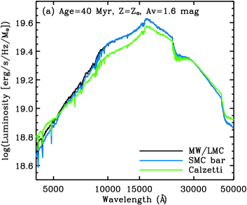
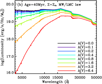
Figure 17: Examples of our adopted combined array of SSP SEDs. (a) SEDs for a 40 Myr old SSP with $Z$ = $Z_{\odot}$, for three different extinction laws and $A_{V}$ = 1.6 mag. Note that over the wavelength range of interest (0.4–3.75 µm), the Milky Way and LMC extinction laws are essentially indistinguishable and were combined; (b) SEDs for a 40 Myr old SSP with $Z$ = $Z_{\odot}$, for eight different extinction values and a MW/LMC extinction law.

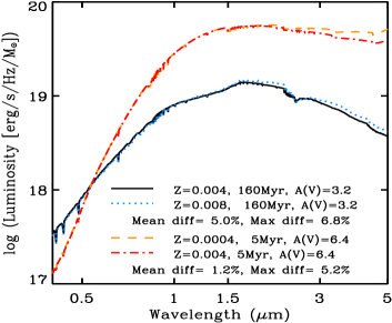
Figure 18: Examples of two pairs of SSP model SEDs that just meet our $\max\{\Delta^{ij}_{k}\}$ or mean$\{\Delta^{ij}_{k}\}$ $>$ 5% criteria for being distinguishable over the 0.4–3.75 µm wavelength range, each normalized at $\lambda$ = 1 µm. The lower pair (black/blue) is for mean$\{\Delta^{ij}_{k}\}$ $>$ 5% and therefore also has $\max\{\Delta^{ij}_{k}\}$ greater than 5%, and the upper pair (red/orange) is for $\max\{\Delta^{ij}_{k}\}$ $>$ 5%.

Within typical observational uncertainties, many of these unique SSP SEDs will be indistinguishable from one or more of the others over the wavelength range of interest. We quantified the differences between each pair of SEDs, where we only need to consider differences in SED shape, not in the absolute flux scale (which depends on the total mass of stars formed). We first divide the 0.4–3.75 µm wavelength range in 10 equal linear bins, and normalize the integrated flux in each bin to the mean integrated flux in all bins. For each pair of SEDs, $(i,j)$, and each wavelength bin, $k$, we compare the difference between normalized integrated fluxes as:

$$\Delta^{ij}_{k}=\left|\,\int_{k}{F_{i}(\lambda)}\middle/\overline{\int_{k}{F_{i}(\lambda)}}\ -\int_{k}{F_{j}(\lambda)}\middle/\overline{\int_{k}{F_{j}(\lambda)}}\,\right|.$$ (A1)

Table 6: Parameter set of our combined SSP model SEDs.

Parameter	Values
$Z$	0.0001, 0.0004,  0.004,  0.008,  0.02, 0.05
Age (Myr)	3,  4,  5,  7,  10,  20,  40,  80,  160,  320,
	640, 1250,  2500,  5000,  10000,  13250
Extinction law	MWa/LMCb, SMCc, Calzettid
$A_{V}$ (mag)	0.0,  0.1,  0.2,  0.4,  0.8,  1.6,  3.2,  6.4

^aFitzpatrick (1999), ^bMisselt et al. (1999), ^cGordon et al. (2003), ^dCalzetti et al. (2000).

We reject SED $j$ as indistinguishable from SED $i$ when both the maximum difference, $\max\{\Delta^{ij}_{k}\}$, and the mean$\{\Delta^{ij}_{k}\}$ are smaller than 5%. Using this criterion, we rejected 1388 of our 2112 SSP SEDs, leaving a set of 724 unique and distinguishable SEDs for further analysis of the $\beta_{V}$ method and its comparison with the SED fitting method, and for fitting observed SEDs of individual regions within galaxies (Jansen et al., in prep.; Kim et al., in prep.). Figure 18 shows two examples of pairs of SEDs that were deemed to be just distinguishable ($>$5%) over the 0.4–3.75µm interval.

Appendix B THE MAGNITUDE OFFSETS BETWEEN AB & VEGA MAGNITUDE SYSTEMS FOR VARIOUS FILTERS

Throughout this study, we use the AB magnitude system (Oke 1974; Oke & Gunn 1983). For observers with data calibrated onto the Vega magnitude system, we here provide magnitude offsets between AB and Vega magnitudes, derived using the Kurucz (1993) Vega spectrum as available in STSDAS 3.16 (www.stsci.edu/institute/software_hardware/stsdas/). We also list the central wavelength, $\lambda_{c}$, and bandwidth (FWHM), $\Delta\lambda$, of each filter in Table 7.

Table 7: Central wavelengths, bandwidths, and magnitude offsets between AB and Vega magnitudes for each of the filters used in the present study.

Filter	$\lambda_{c}$(Å)	$\Delta\lambda$(Å)	$m_{\lambda,\mathrm{AB}}-m_{\lambda,\mathrm{Vega}}$	Filter	$\lambda_{c}$(Å)	$\Delta\lambda$(Å)	$m_{\lambda,\mathrm{AB}}-m_{\lambda,\mathrm{Vega}}$
$B$	4361	890	$-$0.098	WFC3 UVIS F475W	4773	1344	$-$0.088
$V$	5448	840	0.022	WFC3 UVIS F555W	5308	1562	$-$0.013
$R_{c}$	6400	1500	0.213	WFC3 UVIS F606W	5887	2182	0.096
$I_{c}$	7900	1500	0.455	WFC3 UVIS F625W	6242	1463	0.163
$I$	7980	1540	0.436	WFC3 UVIS F775W	7647	1171	0.396
SDSS $g$	4774	1377	$-$0.085	WFC3 UVIS F814W	8024	1536	0.433
SDSS $r$	6231	1371	0.167	WFC3 UVIS F850LP	9166	1182	0.536
SDSS $i$	7615	1510	0.394	WFC3 IR F098M	9864	1570	0.576
SDSS $z$	9132	940	0.530	WFC3 IR F105W	10552	2650	0.660
ACS WFC F435W	4297	1038	$-$0.094	WFC3 IR F110W	11534	4430	0.775
ACS WFC F475W	4760	1458	$-$0.088	WFC3 IR F125W	12486	2845	0.916
ACS WFC F555W	5346	1193	0.006	WFC3 IR F160W	15369	2683	1.267
ACS WFC F606W	5907	2342	0.100	$J$	12546	1620	0.909
ACS WFC F625W	6318	1442	0.178	$H$	16487	2510	1.383
ACS WFC F775W	7764	1528	0.403	$K_{S}$	21634	2620	1.853
ACS WFC F814W	8333	2511	0.438	$K$	22053	3889	1.886
ACS WFC F850LP	9445	1229	0.536	$K^{\prime}$	21218	3404	2.800
WFC3 UVIS F438W	4325	618	$-$0.144
$L$	34831	5103	2.760	NIRCam F410M	40820	4380	3.087
$L^{\prime}$	38333	5880	2.954	NIRCam F444W	44080	10290	3.224
WISE $W$1	33836	7934	2.681	NIRCam F480M	48740	3000	3.423
Spitzer $I$1	35466	7432	2.797	MIRI F560W	56000	12000	3.732
NIRCam F200W	19890	4570	1.691	MIRI F770W	77000	22000	4.352
NIRCam F356W	35680	7810	2.793	MIRI F1000W	100000	20000	4.921

(a) Central wavelength; (b) Width of the bandpass (FWHM); (c) Magnitude offset between AB and Vega magnitude system; $m_{\lambda,\mathrm{AB}}$$-$ $m_{\lambda,\mathrm{Vega}}$= $-$2.5  $\log{(F_{\lambda,\mathrm{Vega}})}$$-$ 48.585 (Hayes & Latham 1975; Bessell & Brett 1988; Bessell 1990; Colina & Bohlin 1994) (d) Bessell (2005); (e) Dressel (2015); (f) Bessell (1979); (g) Gunn et al. (1998); (h) Avila et al. (2015); (i) Cohen et al. (2003); (j) http://www.stsci.edu/jwst/instruments/nircam/instrumentdesign/filters/; (k) http://ircamera.as.arizona.edu/MIRI

Figure 19: Same as Figure 5 for the SDSS $g$, $r$, $i$, and $z$ filters.

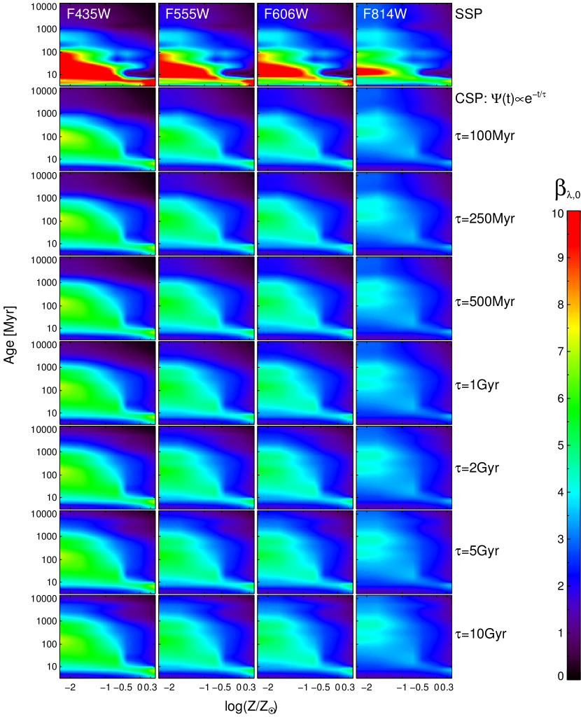
Figure 20: Same as Figure 5 for the HST/ACS WFC F435W, F555W, F606W, and F814W filters.

Figure 21: Same as Figure 5 for the HST/ACS WFC F475W, F625W, F775W, and F850LP filters.

Figure 22: Same as Figure 5 for the HST/WFC3 UVIS F438W, F555W, F606W, and F814W filters.

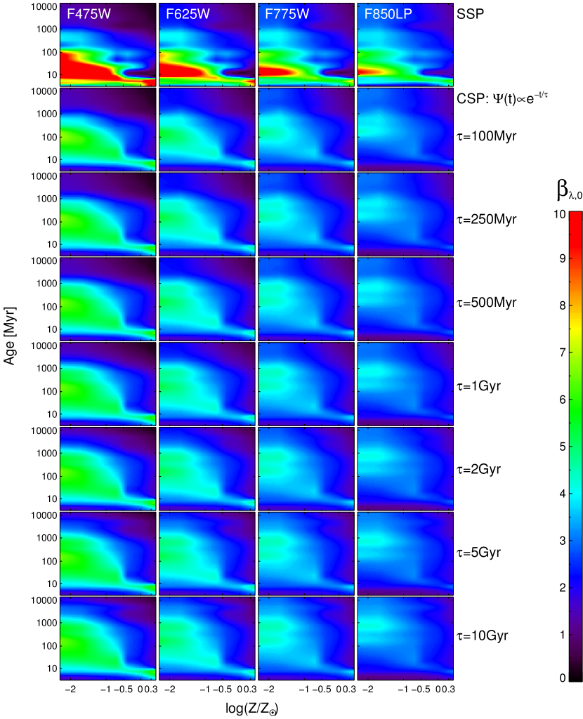
Figure 23: Same as Figure 5 for the HST/WFC3 UVIS F475W, F625W, F775W, and F850LP filters.

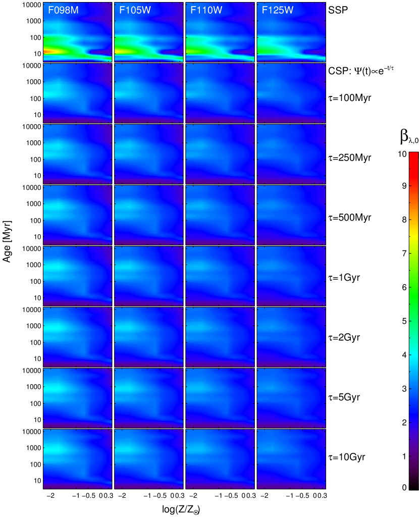
Figure 24: Same as Figure 5 for the HST/WFC3 IR F098M, F105W, F110W, and F125W filters.

(a)  

(b)  

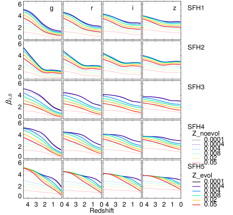
Figure 25: Same as Figure 10 for the SDSS $g$, $r$, $i$, and $z$ filters.

(a)  

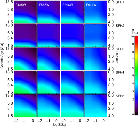
(b)  

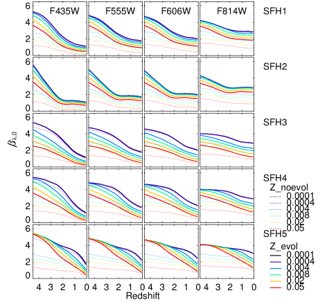
Figure 26: Same as Figure 10 for the HST/ACS WFC F435W, F555W, F606W, and F814W filters.

(a)  

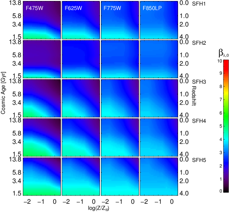
(b)  

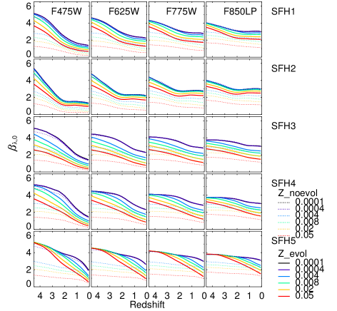
Figure 27: Same as Figure 10 for the HST/ACS WFC F475W, F625W, F775W, and F850LP filters.

(a)  

(b)  

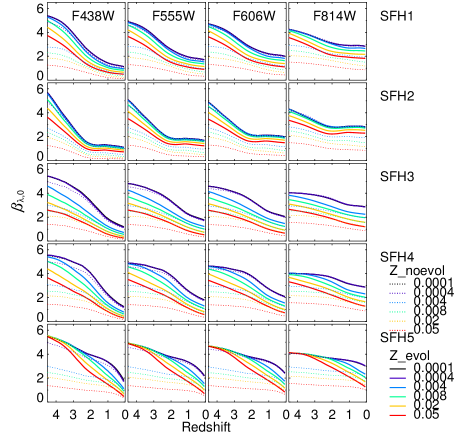
Figure 28: Same as Figure 10 for the HST/WFC3 UVIS F438W, F555W, F606W, and F814W filters.

(a)  

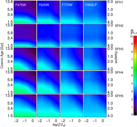
(b)  

Figure 29: Same as Figure 10 for the HST/WFC3 UVIS F475W, F625W, F775W, and F850LP filters.

(a)  

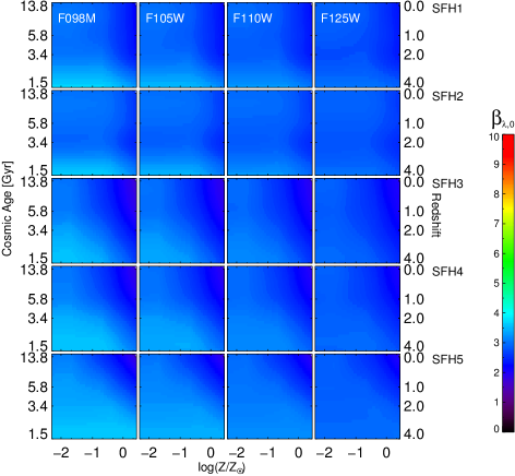
(b)  

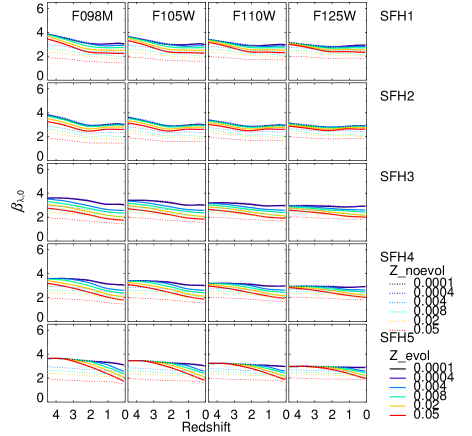
Figure 30: Same as Figure 10 for the HST/WFC3 IR F098M, F105W, F110W, and F125W filters.