Coarse-to-Fine Segmentation With Shape-Tailored Scale Spaces

Abstract

We formulate a general energy and method for segmentation that is designed to have preference for segmenting the coarse structure over the fine structure of the data, without smoothing across boundaries of regions. The energy is formulated by considering data terms at a continuum of scales from the scale space computed from the Heat Equation within regions, and integrating these terms over all time. We show that the energy may be approximately optimized without solving for the entire scale space, but rather solving time-independent linear equations at the native scale of the image, making the method computationally feasible. We provide a multi-region scheme, and apply our method to motion segmentation. Experiments on a benchmark dataset shows that our method is less sensitive to clutter or other undesirable fine-scale structure, and leads to better performance in motion segmentation.

Without Coarse-to-Fine Approach

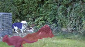
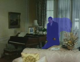
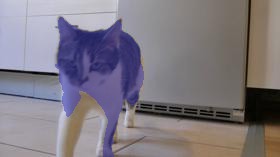
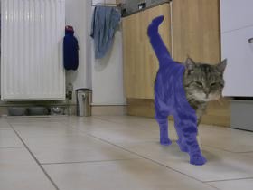
With Our Coarse-to-Fine Approach

Figure 1: Our novel reformulation of existing data terms in segmentation based on scale spaces defined within regions of the segmentation, and integrated over a continuum of scales, leads to a scheme that exhibits a coarse-to-fine property. This leads to less sensitivity of the method to clutter while retaining boundary accuracy.

1 Introduction

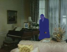
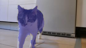
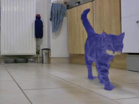
Segmentation of images and videos using low-level cues plays a key role in computer vision. An image consists of many different structures at different scales, and thus the notion of scale space [1], which consists of blurs of the image at all degrees, has been central to computer vision. The need for incorporating scale space in segmentation is well-recognized [2]. Further, there is evidence from human visual studies (e.g., [3, 4]) that the coarse scale, i.e., from high levels of blurring, is predominantly processed before the fine scale. This coarse-to-fine principle has led to many efficient algorithms that are able to capture the coarse structure of the solution, which is often most important in computer vision. Therefore, it is natural for segmentation algorithms to use scale space and operate in a coarse-to-fine fashion.

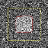
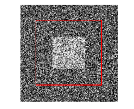
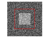
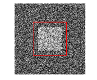
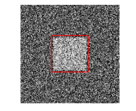
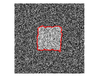
Existing methods for segmentation that incorporate scale have either one of the following limitations. First, most segmentation methods (e.g., [5, 6, 7, 8]) based on scale spaces consider scale spaces that are globally computed on the whole image, which does not capture the fact that there exist multiple regions of the segmentation at different scales, and this could lead to the removal and/or displacement of important structures in the image, for instance, when large structures are blurred across small ones, leading to an inaccurate segmentation. Second, algorithms that use a coarse-to-fine principle (e.g., [9, 10]) do so sequentially (see Figure 2) so that the algorithm operates at the coarser scale and then uses the result to initialize computation at a finer scale. While this warm start may influence the finer scale result, there is no guarantee that the coarse structure of the segmentation is preserved in the final solution.

Contributions: In this paper, we develop an algorithm that simultaneously addresses these two issues. 1. Specifically, we formulate a novel multi-label energy for segmentation that integrates over a continuum scales of scale spaces that are defined within regions of the segmentation, referred to as a Shape-Tailored Scale Space, thus preventing removal or displacement of important structures. By integrating over a continuum of scales of the scale space determined by the Heat Equation, we show that this energy has preference to coarse structure of the data without ignoring the fine structure. 2. Further, we show that the optimization of the energy operates in a parallel coarse-to-fine fashion (see Figure 2). In particular, it considers a continuum of scales together, and it is initially dominated by the coarse structure of the data, then moves to segment finer structure of the data, while preserving the structure obtained from the coarse scale of the data. 3. We apply our algorithm to the problem of segmenting objects in video by motion, and show that we improve an existing method on a benchmark dataset by merely changing the data term in the energy to incorporate our ideas.

Sequential Coarse-to-Fine

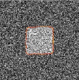
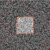
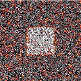
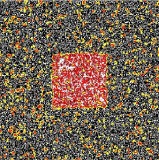
Parallel Coarse-to-Fine (Ours)

Figure 2: [Top]: Sequential coarse-to-fine methods use the result of segmentation (red) from the coarse scale to initialize (yellow) the finer scales, and may lose coarse structure of the coarse segmentation solution without additional heuristics. Note that the result of segmentation of the coarse scale is the left image in red (the blurred image is not shown), and towards the right segmentation is done at finer scales. [Bottom]: Our parallel coarse-to-fine approach considers a continuum of scales all at once and has a coarse-to-fine property. The evolution is shown from left to right.

1.1 Related Work

Scale space theory [1, 11, 12, 13] has a long and rich history as a theory for analyzing images, and we only provide brief highlights. The basic idea is that an image consists of structures at various different scales (e.g., a leaf of a tree exists at a different scale than a forest), and thus to analyze an image without a-priori knowledge, it is necessary to consider the image at all scales. This is accomplished by blurring the image at a continuum of kernel sizes. The most common kernel is a Gaussian, which is known to be the only scale space satisfying certain axioms such as not introducing any new features as the image is blurred [14]. Scale space has been used to analyze structures in images (e.g., [15, 16, 14, 17]). This has had wide ranging applications in stereo and optical flow [18], reconstruction [19, 20], key -point detection in wide-baseline matching [21], design of descriptors for matching [22], shape matching [23], and curve evolution [24], among others.

Gaussian scale spaces have also been used in image segmentation, most notably in texture segmentation [25, 5, 6], which occur frequently in general images [7, 8], where the need for scale information is cogent. While these methods naturally capture important scale information, they use a global scale space defined on the entire image, which blurs across segmentation boundaries. Anisotropic scale spaces [2, 26] have been applied to reduce blurring across boundaries, but this could blur across regions where edges are not salient. Recently, [27] have addressed this issue by using discrete scales computed locally within the evolving regions of the segmentation. However, only a discrete number of scales are used and the method does not exhibit a coarse-to-fine property, which is the focus of this work. Such methods for segmentation have been numerically implemented with various optimization methods, including level sets [28], and more recently convex optimization methods [29]. The energy we consider is not convex, and thus we rely on gradient descent on curves. The energy we consider involves optimization with partial differential equation (PDE) constraints, and thus we apply optimization techniques from [30, 31].

Coarse-to-fine methods, where coarse representations of the image or objective function are processed and then finer aspects of the data are successively revealed, have a long history in computer vision. One such work is [9]. In these methods, data or the objective function is smoothed, and the smoothed problem is solved. The result is used to initialize the problem with less smoothing, where finer details of the data are revealed. The hope is that this result retains aspects of coarse solution, while gradually finding finer detail. However, without additional heuristics such as restricting the finer solution to be around the solution of the coarse problem, there is no guarantee that coarse structure is preserved when solving the finer problem. Recently, [10] provided analysis and derived closed form solutions for the smoothing of the objective in problems of point cloud matching. Our method uses a single energy integrating over a continuum of scales in parallel, and we optimize this energy directly. The optimization is dominated by coarse aspects of the data without ignoring fine aspects initially. Then fine aspects become more prominent, but the coarse structure is preserved without any heuristics.

Since we apply our method to the problem of segmenting moving objects in video based on motion, we highlight some aspects of that literature most relevant to this work. Methods for motion segmentation are based on optical flow (e.g., [32]). Piecewise parametric models for motion of regions in segmentation are used in e.g., [33, 34]. Non-parametric warps are used for motion models (e.g.,[35, 36, 37]). Our goal here is not to estimate motion, but rather we use existing techniques for motion estimation, and improve the segmentation of regions by replacing the data term with our novel energy.

2 Energy and Optimization

In this section, our goal is to construct the energy with preference to segmenting the coarse structure of the image(s) over finer structure, without losing the ability to include fine-scale structure in the segmentation. We use a scale space defined within regions of the image, called a Shape-Tailored Scale Space, which computes coarse-structure of the data without blurring across region boundaries, to construct the energy. Finally, we show that in optimizing the energy, which requires multiple scales to define, it is not necessary to compute multiple scales of the data, providing a convenient implementation using the natural resolution of the image.

2.1 Shape-Tailored Heat Scale Space

The Gaussian Scale Space (see Figure 3), constructed by smoothing the image with a Gaussian at a continuum of scales (variances), has been shown to be the only scale space satisfying natural axiomatic properties, which includes non-creation of new structures in the data with increasing scale. The last property implies that increasing scales represent coarser representations of the data. The Gaussian Scale Space can be generalized to be defined within regions (subsets of the image) of arbitrary shape by using the Heat Equation. The solution to the Heat Equation defaults to Gaussian smoothing when the domain is $\mathbb{R}^{2}$, and approximately so when the domain is a rectangle, as in an image. The Heat Equation, defined in a region $R$, is defined as follows:

$$\begin{cases}\partial_{t}u(t,x)=\Delta u(t,x)&x\in R,\,t>0\\ \nabla u(t,x)\cdot N=0&x\in\partial R,\,t>0\\ u(0,x)=I(x)&x\in R\end{cases}$$ (1)

where $u:[0,+\infty)\times R\to\mathbb{R}^{k}$ denotes the scale space, $R\subset\Omega\subset\mathbb{R}^{2}$ is the domain (or subset) of the image $\Omega$, $I$ is the image, $\partial R$ denotes the boundary of $R$, $N$ is the unit outward normal vector to $R$, $\nabla$ denotes the vector of partials, $\Delta$ denotes the Laplacian, $\partial_{t}$ denotes the partial derivative with respect to $t$, and $t$ is the scale parameter parameterizing the scale space. Note that $t$ is related to $\sigma$, the standard deviation of the Gaussian kernel, by $\sigma=\sqrt{2t}$, in the case the domain is $\mathbb{R}^{2}$.

$t=0$	$t=50$	$t=100$	$t=150$	$t=200$

Figure 3: Gaussian scale space (solution of Heat Equation) for various times (scales). Notice the quick diffusion of fine scale structures, and the persistence of coarse structure over much of the scale space. The persistence of coarse structure is important in defining our coarse-to-fine segmentation scheme.

This construction of the Gaussian Scale Space using the Heat Equation is particularly useful for segmentation, as it allows us to conveniently compute coarse representations of the data when $R$ is a region of a segmentation. By using the PDE in (1), we may naturally smooth only within an arbitrary shaped subset of the image without integrating information across the region boundary. If the regions are chosen to be the correct segmentation, this avoids blurring data across segmentation boundaries. However, one does not know the segmentation a-priori, and thus the regions are simultaneously estimated together with the scale spaces within the regions in the optimization problem that we define next.

2.2 Coarse-Scale Preferential Energy

A property of the Gaussian scale space that is relevant in defining our coarse-scale preferential energy is that the Heat Equation removes the fine structure of the image in short time, and spends more of its time removing coarse structure (see Figure 3). Therefore, integrating a data term in segmentation problems over the scale parameter of the Heat Equation, would give preference to segmentations that separate the coarse structure of the image without ignoring contributions from the fine structure. This intuition leads us to construct the following segmentation energy defined on possible segmentations of the domain as a data term:

$$E(\{R_{i}\}_{i=1}^{N})=\sum_{i=1}^{N}E_{i}(R_{i}),\quad E_{i}(R_{i})=\int_{0}^{T}\int_{R_{i}}|u_{i}(t,x)-a_{i}|^{2}\,\mathrm{d}x\,\mathrm{d}t,$$ (2)

where $T>0$ is the final time, $\{R_{i}\}_{i=1}^{N}$ are a collection of regions forming the segmentation, and $a_{i}\in\mathbb{R}^{k}$ is the average value of $u_{t}$ within $R_{i}$. It can be shown that $a_{i}$ is independent of $t$. The parameter $T$ will be eliminated below as we take the limit as $T\to\infty$ . This energy is the mean-squared error of the image within the region across all scales. It generalizes common single scale segmentation models, including piecewise constant Mumford-Shah (Chan-Vese [38]), and piecewise smooth Mumford-Shah [39]. Note that one way to generalize the latter is by taking the initial condition for the Heat Equation (1) as $I-f$ where $f$ is a smooth version of $I$; this results in $a_{i}=0$. We will see in Section 3 that it also generalizes motion segmentation models.

To further justify the intuition that the energy chooses regions so that coarse structure of the image has more influence than the fine structure, we analyze a term of the energy above in Fourier domain. Since Fourier analysis is convenient in rectangular domains, we analyze the energy when the region is $R_{i}=\mathbb{R}^{2}$. In this case, the energy can be written in terms of its Fourier transform as:

Lemma 1

Suppose $I:\mathbb{R}^{2}\to\mathbb{R}$ and $a=\int_{\mathbb{R}^{2}}I(x)\,\mathrm{d}x=\int_{\mathbb{R}^{2}}u(t,x)\,\mathrm{d}x$. Then

$$E=\int_{0}^{\infty}\int_{\mathbb{R}^{2}}|u(t,x)-a|^{2}\,\mathrm{d}x\,\mathrm{d}t=\int_{\mathbb{R}^{2}}|H(\omega)\hat{I}(\omega)|^{2}\,\mathrm{d}\omega,\,\,\mbox{where }H(\omega)=\frac{1}{\sqrt{2}|\omega|},$$ (3)

where $\hat{I}$ denotes the Fourier transform, and $\omega$ denotes frequency.

The proof is a straight forward application of Parseval’s Theorem, details of which can be found in Supplementary materials. The function $H$ decays the high frequency components of $I$ at a linear rate, thus the energy gives preference to the coarse image structure. Note that without integrating over the scale space, the energy in Fourier domain has the same expression, except with $H=1$, thus having equal preference to both coarse and fine structure. Since Fourier analysis is not particularly simple for regions that are not rectangular, the original energy is not formulated in Fourier domain. However, we show in the next sub-section that the optimization of the energy using the scale-space can be expressed without computing the entire scale space, which is convenient in implementation.

2.3 Constrained Optimization Problem

The energy of interest (2) is a function of regions, and thus we design an optimization scheme with respect to the regions. Since the integrand of the energy depends on the regions nonlinearly, as the Heat Equation is a function of the region, the energy is not convex, and thus we apply gradient descent. In order to compute the gradient, we formulate the energy minimization as a constrained optimization problem. That is, we treat the minimization of the energy (2) as defined on both the regions $R_{i}$ and $u_{i}$ with the constraint that $u_{i}$ satisfies the Heat Equation (1). This formulation allows us to apply the technique of Lagrange multipliers, which makes computations simpler. In particular, the technique allows us to decouple the nonlinear dependence of $u_{i}$ on $R_{i}$, since the latter variables can be treated independently.

Since all terms of the energy (2) have the same form, we focus on computing the gradient for any one term. For convenience in notation, we avoid the subscript $i$ denoting the index of the region. We may formulate the energy as a function of region $R$, $u$, and a Lagrange multiplier $\lambda:[0,T]\times R\to\mathbb{R}^{k}$ with the constraint that $u$ satisfies the Heat Equation:

$$E(R,u,\lambda)=\int_{0}^{T}\int_{R}f(u)\,\mathrm{d}x\,\mathrm{d}t+\int_{0}^{T}\int_{R}\left(\nabla\lambda\cdot\nabla u+\lambda\partial_{t}u\right)\,\mathrm{d}x\,\mathrm{d}t.$$ (4)

We have excluded the dependencies on $x,t$ for convenience of notation. We have also provided a more general form of the squared error with a general function $f$ of $u$. The second term comes from the weak form of the Heat Equation. Note that integrating by parts to move the gradient from $\lambda$ to $\nabla u$ gives the classical form of the Heat Equation in (1). Therefore, the second term is indeed obtained by the usual Lagrange multiplier technique.

We may now compute the gradient for $E$ (4) by deriving the optimizing conditions in $u$ and $\lambda$. Optimizing in $\lambda$ simply results in the original Heat Equation constraint, so we compute the optimizing condition for $u$ by computing the derivative (variation) of $E$ with respect to $u$. This results in a solution for $\lambda$ as given below:

Lemma 2

The Lagrange multiplier $\lambda$ satisfies the following Heat Equation with forcing term, evolving backwards in time:

$$\begin{cases}\partial_{t}\lambda(t,x)+\Delta\lambda(t,x)=f^{\prime}(u(t,x))&x\in R\times[0,T]\\ \nabla\lambda(t,x)\cdot N=0&x\in\partial R\times[0,T]\\ \lambda(T,x)=0&x\in R\end{cases}.$$ (5)

The solution of this equation can be expressed with Duhamel’s Principle [40] as

$$\lambda(t,x)=-\int_{t}^{T}F(s-t,x;s)\,\mathrm{d}s.$$ (6)

where $F(\cdot,\cdot;s):[0,T]\times R\to\mathbb{R}$ is the solution of the forward heat equation (1) with zero forcing and initial condition $f^{\prime}(u)$ evaluated at time $s$, i.e.,

$$\begin{cases}\partial_{t}F(t,x;s)-\Delta F(t,x;s)=0&x\in R\times[0,T]\\ \nabla F(t,x;s)\cdot N=0&x\in\partial R\times[0,T]\\ F(0,x;s)=f(s,x)&x\in R\end{cases}.$$ (7)

In the case that $f(u)=(u-a)^{2}$, $\lambda$ can be expressed as

$$\lambda(t,x)=-2\int_{t}^{T}(u(2s-t,x)-a)\,\mathrm{d}s.$$ (8)

The formula for $\lambda$ in (8) is convenient as a numerical integration scheme is no longer required after computation of the scale space $u$.

With the optimizing conditions for $u$ and $\lambda$ of $E$, we can now compute the gradient of the energy $E$ with respect to $R$ in terms of $\lambda$ and $u$:

Proposition 1

The gradient of $E$ with respect to the boundary $\partial R$ can be expressed as

$$\nabla_{\partial R}E=\int_{0}^{T}\left[f(u)+\nabla\lambda\cdot\nabla u+\lambda\partial_{t}u\right]\,\mathrm{d}t\cdot N,$$ (9)

where $N$ is the normal vector to $\partial R$. In the case that $f(u)=(u-a)^{2}$ and as $T$ gets large, the gradient approaches

$$\nabla_{\partial R}E=\left(-\frac{1}{2}|\nabla\lambda(0)|^{2}-\lambda(0)[u(0)-a]\right)N,\quad\lambda(0,x)=-\int_{0}^{2T}(u(s,x)-a)\,\mathrm{d}s,$$ (10)

where $\lambda(0)$ and $u(0)$ denote the functions $\lambda$ and $u$ at time zero.

The simplification in (10) of the gradient is particularly convenient since it only involves explicit functions of the scale space $u$. More conveniently, we may express $\lambda(0)$ as the solution of the Poisson equation at the native scale of the image so that it is not necessary to compute the whole scale space $u$ to evaluate the gradient (10):

Lemma 3

As $T$ gets large, $\lambda(0)$ defined in (10) approaches the solution of the Poisson equation:

$$\begin{cases}-\Delta\lambda(0,x)=a-u(0,x)&x\in R\\ \nabla\lambda(0,x)\cdot N=0&x\in\partial R\\ \mbox{avg}({\lambda(0)})=0\end{cases},$$ (11)

where $\mbox{avg}({\lambda(0)})=\frac{1}{|R|}\int_{R}\lambda(0,x)\,\mathrm{d}x$ is the average value over $R$, and $|R|$ is the area of $R$.

Proof

Since the proof is short, we provide it here:

$$\Delta\lambda(0)=-\Delta\int_{0}^{2T}(u(s)-a)\,\mathrm{d}s=-\int_{0}^{2T}\Delta u(s)\,\mathrm{d}s=-\int_{0}^{2T}\partial_{s}u(s)\,\mathrm{d}s\\ =-(u(2T)-u(0))\to-(a-u(0))\mbox{ as }T\to\infty.$$

In practice, taking $T$ all the way to infinity may enforce too much of the coarse structure, and in segmenting objects with fine details, the evolution may take too long to finally determine the fine scale structure. Thus, rather than taking $a$ to approximate $u(2T)$ in the above computation, we instead approximate it with the solution of the equation:

$$\begin{cases}v(x)-\alpha\Delta v(x)=I(x)&x\in R\\ \nabla v(x)\cdot N=0&x\in\partial R\end{cases},$$ (12)

which smooths $I$ (larger $\alpha$ smooths $I$ more and can be regarded as a maximum scale parameter). For a fixed scale, this solution qualitatively behaves similar to the Heat Equation (they are both low-pass filters). In experiments, this approximation still gives the desired coarse-to-fine behavior. Solving (11) with right hand side $v-u(0)$ and $\alpha$ set to the maximum desirable scale approximates $-\int_{0}^{2T}(u(t,x)-a)\,\mathrm{d}t$ for finite $T$. We set $\alpha=20$ in experiments. The reason for using the equation $v-\alpha\Delta v=I$ is that it is computationally less costly to solve than solving the Heat Equation directly, and it allows for fast updates as the regions evolve using the solution from the previous iteration as a warm start.

In summary, we compute the solution of the Poisson equation (11) with right hand side $v-u(0)$ at the native scale of the image to solve for $\lambda(0)$ in the computation of an approximate gradient of $E_{i}$ in (2). Then, the gradient is computed using the formula in (10) that requires only simple operations (partial derivatives, squaring, etc). Therefore, the effects of the scale space are compressed into two equations at the native scale of the image.

2.4 Multi-label Scheme and Implementation

We now present a method for implementing the gradient flow derived in the previous section. Since we are interested in applications with possibly many regions in the segmentation of the image, we present a method for implementing the gradient flow when there are $N$ regions. To achieve sub-pixel accuracy, we use relaxed indicator functions $\phi_{i}:\Omega\to[0,1]$ with $i=1,\ldots,N$ to represent the regions. Denote by $G_{i}$ the quantity (10) multiplying the normal vector for region $R_{i}$:

$$G_{i}=-\frac{1}{2}|\nabla\lambda_{i}(0)|^{2}-\lambda_{i}(0)[u_{i}(0)-a],\quad\mbox{in }D(R_{i})$$ (13)

where $D(R_{i})$ is a small dilation of $R_{i}$ and $\lambda_{i}(0)$ is the solution of (11) computed in this set. The extension beyond the region is done so that the evolution of $\phi_{i}$ can be defined around the curve, as in level set methods [28]. We can now derive the updated scheme for the $\phi_{i}$ so that the zero level set evolves in such a way that it matches the curve evolution induced by the gradient descent. This is given in Algorithm 1.

1:Input: An initialization of $\phi_{i}$

2:repeat

3:     Compute regions: $R_{i}=\{x\in\Omega\,:\,i=\mbox{argmax}_{j}\phi_{j}(x)\}$

4:     Dilated regions $R_{i}$: $D(R_{i})$

5:     Compute $\lambda_{i}$ in $D(R_{i})$ by solving the Poisson equation (11)

6:     Compute $G_{i}$ for band pixels $B_{i}=D(R_{i})\cap D(\Omega\backslash R_{i})$

7:     Update pixels $x\in D(R_{i})\cap D(R_{j})$ as follows:

$$\phi_{i}^{\tau+\Delta\tau}(x)=\phi_{i}^{\tau}(x)-\Delta\tau(G_{i}(x)-G_{j}(x))|\nabla\phi_{i}^{\tau}(x)|+\varepsilon\Delta\phi_{i}^{\tau}(x).$$

8:     Update all other pixels as

$$\phi_{i}^{\tau+\Delta\tau}(x)=\phi_{i}^{\tau}(x)+\varepsilon\Delta\phi_{i}^{\tau}(x).$$

9:     Clip values between 0 and 1: $\phi_{i}=\max\{0,\min\{1,\phi_{i}\}\}$.

10:until  regions have converged

Algorithm 1 Multi-label Gradient Descent

The update of the $\phi_{i}$ in Line 7 of Algorithm 1 involves the term $\Delta\phi_{i}^{\tau}$, which provides smoothness of the curve. More sophisticated regularizers (such as length regularization) may be used, but we have found this simple regularization sufficient. We choose $\varepsilon=0.005$ in experiments, and this does not need to be tuned, as it is mainly for inducing regularity for computation of derivatives of $\phi$.

3 Application to Motion Segmentation

In this section, we show how the results of the previous section can be applied to motion segmentation. Motion segmentation is the problem of segmenting objects and/or regions with similar motions computed using multiple images of the object(s). One of the challenges of motion segmentation is that motion is inferred typically through a sparse set of measurements (e.g., along image edges or corners), and thus the motion signal is typically reliable for segmentation in sparse locations. By using a scale space formulation of an energy for motion segmentation, coarse representations of the motion signal are integrated and more greatly impact the segmentation. This property increases the reliability of motion segmentation (Figure 4), and the coarse-to-fine approach captures the coarse-structure without being impacted by fine-scale distractions at the outset.

residual	ctf residual	non-ctf	ctf	non-ctf	ctf

Figure 4: Motion residuals at a single scale are sparse (left column), leading to difficulties in using these cues in segmentation (non-ctf). Motion cues at a continuum of scales (ctf) provide a richer signal (2nd column), which increases reliability in using such cues for segmentation. Segmentations (in purple) are shown for a frame (middle two) and a few frames ahead (right two). Although errors in the non-ctf approach are subtle between frames, they quickly propagate across frames, compared to our approach.

With this motivation, we reformulate the motion segmentation problem with scale space. Let $I_{0},I_{1}:\Omega\to\mathbb{R}^{k}$ be two images of a sequence where $\Omega$ is the domain of the image. For a given region $R_{i}$, we define a mapping $w_{i}:R_{i}\to\Omega\subset\mathbb{R}^{2}$, which we call a warp or deformation that back warps $I_{1}$ to $I_{0}$. We assume that $I_{0}$ and $I_{1}$ are related through $w_{i}$ by the Brightness Constancy Assumption, except for occlusions, as in typical works in the optical flow literature [32]. Define the pointwise error of $w_{i}$ as

$$\mbox{Res}_{i}(x)=\rho(|I_{1}(w_{i}(x))-I_{0}(x)|),\quad x\in R_{i},$$ (14)

where $\rho$ is a robust norm (for instance a truncated linear function) to deal with the effects of deviations from Brightness Constancy [32]. We refer to this quantity as the residual. We would like to formulate an energy defined on possible segmentations to reduce the residual and incorporate our coarse-to-fine approach:

$$E_{mseg}(\{R_{i}\}_{i=1}^{N})=\sum_{i=1}^{N}|\mbox{avg}({\mbox{Res}_{i}})|^{2}+\int_{0}^{T}\int_{R_{i}\backslash O_{i}}(u_{i}(t,x)-\mbox{avg}({\mbox{Res}_{i}}))^{2}\,\mathrm{d}x\,\mathrm{d}t,$$ (15)

where $O_{i}$ is the occluded part of $R_{i}$, $\mbox{avg}({\mbox{Res}_{i}})$ is the mean value of the residual in $R_{i}\backslash O_{i}$, and $u_{i}:[0,T]\times R_{i}\to\mathbb{R}^{+}$ is the scale space of the residual in $R_{i}\backslash O_{i}$. We subtract the mean value of the residual from the scale space so that it fits in the form of (2), and since we would like to reduce the overall residual, we add the mean value of the residual outside the integrand so that it is minimized as well. Had we not subtracted the mean value and not integrated over scale and instead used only the native scale, this would be the usual robust formulation of motion segmentation (e.g., [36]).

Because of the ambiguity of computing motion in occluded and textureless regions, additional terms must be added to the energy, for instance, terms involving fidelity to local appearance histograms. We follow the formulation in [37] to account for these ambiguities, which uses an additional term with fidelity to color histograms in the segmentation energy. Based on the reliability of the motion residuals, the approach switches between segmentation by residuals and color histograms. We simply replace the classical motion term (at a single scale) with our term (15). We do not integrate the color histogram energy over scales, as our goal is to rely less on this term by improving the motion reliability. The optimization involves iterative updates of the warps, occlusion, and the regions. The technique we introduced only affects the updates of the regions, replacing the gradient of the usual single scale motion residual with the gradient of (15) computed by (13), and implemented using Algorithm 1. We apply our method frame-by-frame segmenting a frame using one frame ahead and one frame behind (so that backward motion is also used in segmentation). Then we propagate the result to the next frame via the computed motion to warm-start the segmentation in the next frame.

4 Experiments

	Training set (29 sequences)				Test set (30 sequences)
	P	R	F	$N/65$	P	R	F	$N/69$
[41]	79.17	47.55	59.42	4	77.11	42.99	55.20	5
[35]	81.50	63.23	71.21	16	74.91	60.14	66.72	20
[42]	85.00	67.99	75.55	21	82.37	58.37	68.32	17
[42]+backward	83.00	70.10	76.01	23	77.94	59.14	67.25	15
[43]-Mce S(8), p(.6)	86.91	71.33	78.35	25	87.57	70.19	77.92	25
[43]-Mce S(4), p(.5)	86.79	73.36	79.51	28	86.81	67.96	76.24	25
[43]-Mce D(4), p(.5)	85.31	68.70	76.11	24	85.95	65.07	74.07	23
non-ctf [37]	89.53	70.74	79.03	26	91.47	64.75	75.82	27
ctf (ours)	93.04	72.68	81.61	29	95.94	65.54	77.87	28

Table 1: FBMS-59 results. Average precision (P), recall (R), F-measure (F), and number of objects detected (N) over all sequences in training and test datasets. Higher values indicate superior performance. [42], [37] and our method are frame-to-frame methods; other methods process the video in batch. All methods are fully automatic.

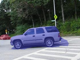
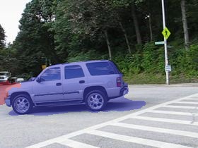
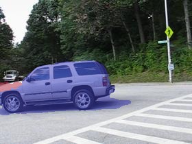
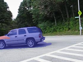
Frames for Increasing Time $\rightarrow$
non-ctf ours non-ctf ours non-ctf ours non-ctf ours non-ctf ours non-ctf ours non-ctf ours

Figure 5: Sample visual results on representative sequences for the FBMS-59 dataset (segmented objects in purple and red). The change of energy to integrate over all scales (our approach) is generally less sensitive to clutter than using an energy that contains only one scale (non-ctf).

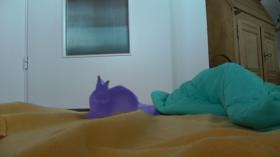
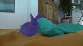
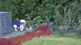
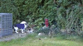
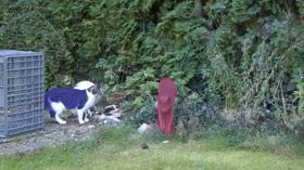
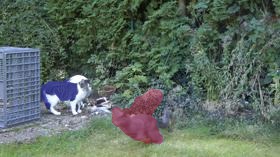
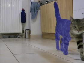
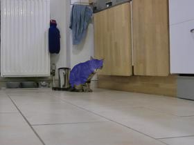
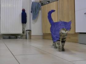
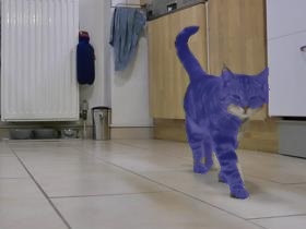
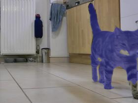
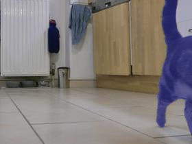
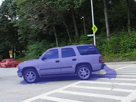
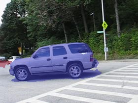
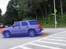
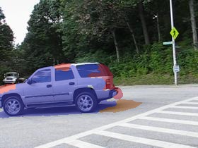
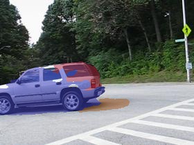
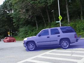
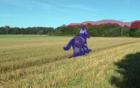
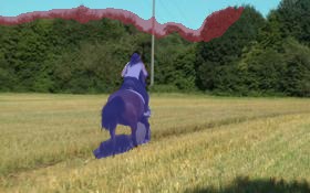
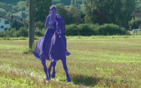
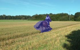
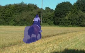
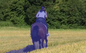
We test our method on a recent benchmark dataset that contains moving objects: the Freiburg-Berkeley Motion Segmentation (FBMS-59) [35] dataset. FBMS-59 consists of two sets - training, 29 sequences, and test, 30 sequences. Videos range between 19 and 800 frames, and have multiple objects.

Evaluation: FBMS-59 measures the accuracy versus ground truth of a subset of frames, ranging from 3 to 41 for each video. The segmentation is measured in terms of region metrics that are measured using precision, recall, $F$ - measure, and the number of objects with $F\geq 0.75$.

Comparison: To demonstrate the advantage of our coarse-to-fine energy over a corresponding single scale energy, we compare to [37]. Our approach replaces the single scale motion term in [37] with the coarse-to-fine energy described in the previous section. Since we test on benchmarks, we also compare to other state-of-the-art approaches, although our main purpose is to show the improvements that occur by merely using our coarse-to-fine energy.

Parameters: We use the parameters in the method [37] provided in their online code, which are chosen constant across all sequences and datasets. Our method requires one parameter $\alpha$ in (12). We choose it to be $\alpha=20$ by selecting it based on a few sequences from the training set. The parameters of [37] are reported to be chosen by using the training set of FBMS-59.

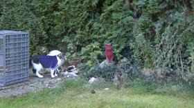
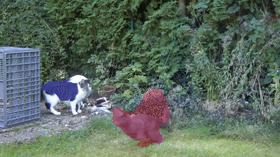
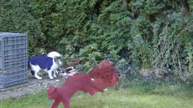
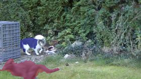
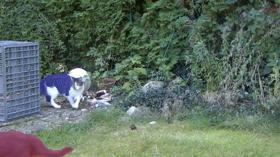
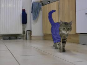
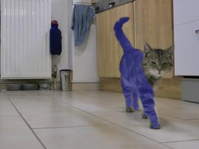
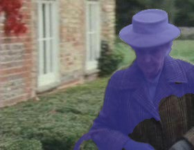
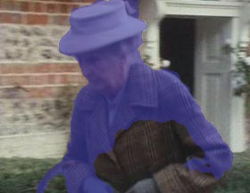
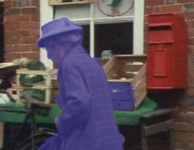
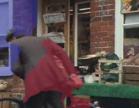
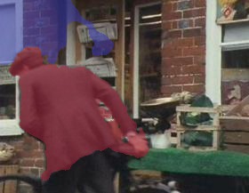
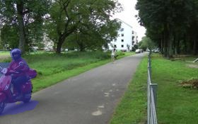
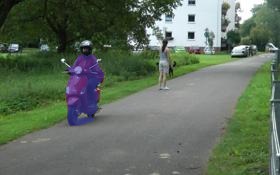
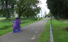
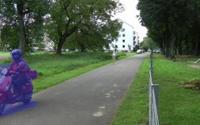
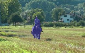
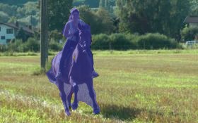
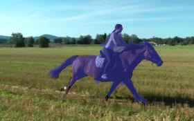
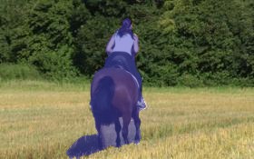
Results on FBMS-59: Figure 5 shows some representative visual results of our method and [37]. Table 1 shows quantitative results of the two approaches, as well as other state-of-the-art methods. Note our method is initialized as in [37] with a clustering of optical flow over several frames. Visual results show our approach generally avoids distracting clutter and thus prevents leakages in comparison to [37]. In many cases, it also captures more of the object. The latter can be attributed to the fact that our approach makes the motion signal more reliable, and thus it is used more frequently than [37], which switches to color histogram segmentation when motion cues are unreliable. Quantitative results show that we improve the F-measure of [37] by about $2\%$ on both training and test sets, and that we increase the number of objects detected. We also have highest F-measure on the training set of all competing methods. On the test set, we are out-performed by [43] by a slim margin of $0.05\%$ F-measure, but we do detect more objects. Note however, [43] and our method are not directly comparable since in [43] the video is processed in batch, whereas our method processes the video frame-by-frame.

Computational cost: The processing required for our approach is small compared with the overall cost of [37]. Our approach requires the solution of a linear equation (11) at each update of the regions, but the solution does not change much between updates and so the solution from the previous iteration provides a good initialization to the current iteration. Our approach adds about 5 secs per frame to the total time on average of about 30 secs per frame by [37] on a 12-core processor.

5 Conclusion

We have presented a general energy that reformulates conventional data terms in segmentation problems. This novel energy incorporates scale space and consists of two important properties: scales spaces are defined on regions, so that structures in different segments are not blurred across nor displaced, and it exhibits a coarse-to-fine property. The latter favors that the coarse structure of the desired segmentation is obtained while finer structure becomes successively obtained, without having to rely on heuristics to maintain that finer solutions remain close to the coarse solution. Our method is based on the Heat Equation defined on regions, and this equation was demonstrated to have the desired properties. We have shown application to the problem of motion segmentation, where relying on data from a single scale is often unreliable. In this case, other information such as color histograms must be used. However, it is often difficult to obtain objects with complex appearance by using color histograms, thus improving reliability of the motion signal segments objects. Experiments on benchmark datasets have shown that our technique improves an existing segmentation method merely by replacing the data term of the motion residual at a single scale with an integration over a continuum of scales. In particular, we observe that our technique is less sensitive to clutter, and many times increases the recall by relying more on motion cues.

Appendix 0.A Proofs of Lemmas and Propositions

Lemma 1

Suppose $I:\mathbb{R}^{2}\to\mathbb{R}$ and $a=\mbox{avg}({I})=\mbox{avg}({u(t,\cdot)})$. Then

$$E=\int_{0}^{\infty}\int_{\mathbb{R}^{2}}|u(t,x)-a|^{2}\,\mathrm{d}x\,\mathrm{d}t=\int_{\mathbb{R}^{2}}|H(\omega)\hat{I}(\omega)|^{2}\,\mathrm{d}\omega,\,\,\mbox{where }H(\omega)=\frac{1}{\sqrt{2}|\omega|},$$ (16)

where $\hat{I}$ denotes the Fourier transform, and $\omega$ denotes frequency.

Proof

Taking the Fourier transform of the Heat Equation:

$$\begin{cases}\partial_{t}u(t,x)=\Delta u(t,x)&x\in\mathbb{R}^{2}\\ u(0,x)=I(x)&t=0\end{cases}$$

yields:

$$\partial_{t}\hat{u}(t,\omega)=(i\omega)\cdot(i\omega)\hat{u}(t,\omega)=-|\omega|^{2}\hat{u}(t,\omega),$$

where $\hat{u}(t,\omega)$ is the Fourier transform of $u$. Solving this differential equation yields

$$\hat{u}(t,\omega)=e^{-|\omega|^{2}t}\hat{I}(\omega).$$

We note that $a=0$ when $I\in\mathbb{L}^{2}$ since $\hat{I}(0)=\int_{\mathbb{R}^{2}}I(x)\,\mathrm{d}x$ is finite. Then by Parseval’s Theorem,

$$E =\int_{0}^{\infty}\int_{\mathbb{R}^{2}}|u(t,x)-a|^{2}\,\mathrm{d}x\,\mathrm{d}t=\int_{0}^{\infty}\int_{\mathbb{R}^{2}}|\hat{u}(t,\omega)|^{2}\,\mathrm{d}\omega\,\mathrm{d}t$$ (17)

$$=\int_{\mathbb{R}^{2}}\int_{0}^{\infty}e^{-2|\omega|^{2}t}\,\mathrm{d}t\cdot|\hat{I}(\omega)|^{2}\,\mathrm{d}\omega$$ (18)

$$=\int_{\mathbb{R}^{2}}\left.-\frac{1}{2|\omega|^{2}}e^{-2|\omega|^{2}t}\right|_{t=0}^{t=+\infty}|\hat{I}(\omega)|^{2}\,\mathrm{d}\omega=\int_{\mathbb{R}^{2}}\frac{1}{2|\omega|^{2}}|\hat{I}(\omega)|^{2}\,\mathrm{d}\omega$$ (19)

$$=\int_{\mathbb{R}^{2}}|A(\omega)\hat{I}(\omega)|^{2}\,\mathrm{d}\omega$$ (20)

where $A(\omega)=1/(\sqrt{2}|\omega|)$.

Lemma 2

The Lagrange multiplier $\lambda$ satisfies the following Heat Equation with forcing term, evolving backwards in time:

$$\begin{cases}\partial_{t}\lambda(t,x)+\Delta\lambda(t,x)=f^{\prime}(u(t,x))&x\in R\times[0,T]\\ \nabla\lambda(t,x)\cdot N=0&x\in\partial R\times[0,T]\\ \lambda(T,x)=0&x\in R\end{cases}.$$ (21)

The solution of this equation can be expressed with Duhamel’s Principle [40] as

$$\lambda(t,x)=-\int_{t}^{T}F(s-t,x;s)\,\mathrm{d}s.$$ (22)

where $F(\cdot,\cdot;s):[0,T]\times R\to\mathbb{R}$ is the solution of the forward heat equation Eqn. (1) (in the paper) with zero forcing and initial condition $f^{\prime}(u)$ evaluated at time $s$, i.e.,

$$\begin{cases}\partial_{t}F(t,x;s)-\Delta F(t,x;s)=0&(t,x)\in[0,T]\times R\\ \nabla F(t,x;s)\cdot N=0&x\in[0,T]\times\partial R\\ F(0,x;s)=f(u(s,x))&x\in R\end{cases}.$$ (23)

In the case that $f(u)=(u-a)^{2}$, $\lambda$ can be expressed as

$$\lambda(t,x)=-2\int_{t}^{T}(u(2s-t,x)-a)\,\mathrm{d}s.$$ (24)

Proof

We define

$$E(R,u,\lambda)=\int_{R}\int_{0}^{T}f(u)\,\mathrm{d}x\,\mathrm{d}t+\int_{R}\int_{0}^{T}\left(\nabla\lambda\cdot\nabla u+\lambda\cdot u_{t}\right)\,\mathrm{d}x\,\mathrm{d}t.$$ (25)

Integrating by parts, we have that

$$E =\int_{R\times[0,T]}\left[f(u)-(\partial_{t}\lambda+\Delta\lambda)u\right]\,\mathrm{d}x\,\mathrm{d}t$$ (26)

$$+\int_{R}\left.\lambda u\right|_{t=0}^{t=T}\,\mathrm{d}x+\int_{\partial R\times[0,T]}(\nabla\lambda\cdot N)u\,\mathrm{d}s(x)\,\mathrm{d}t,$$ (27)

where $\,\mathrm{d}s$ denotes the arc-length measure of $\partial R$, and $N$ is the unit outward normal of $\partial R$. Differentiating $E$ in the direction (perturbation) $\tilde{u}$ of $u$ evaluated at $u$ yields

$$\,\mathrm{d}E(u)\cdot\tilde{u} =\int_{R\times[0,T]}\left[f^{\prime}(u)-(\partial_{t}\lambda+\Delta\lambda)\right]\tilde{u}\,\mathrm{d}x\,\mathrm{d}t$$ (28)

$$+\int_{R}\left.\lambda\tilde{u}\right|_{t=0}^{t=T}\,\mathrm{d}x+\int_{\partial R\times[0,T]}(\nabla\lambda\cdot N)\tilde{u}\,\mathrm{d}s(x)\,\mathrm{d}t.$$ (29)

Note that $\tilde{u}(0)=0$ since $u(0)=I$ is fixed and thus may not be perturbed. We may choose $\nabla\lambda\cdot N=0$ on $\partial R$ and $\lambda(T)=0$. We are interested in $u$ such that $\,\mathrm{d}E(u)\cdot\tilde{u}=0$ for all $\tilde{u}$. This yields the condition that

$$\begin{cases}\partial_{t}\lambda(t,x)+\Delta\lambda(t,x)=f^{\prime}(u(t,x))&x\in R\times[0,T]\\ \nabla\lambda(t,x)\cdot N=0&x\in\partial R\times[0,T]\\ \lambda(T,x)=0&x\in R\end{cases}.$$ (30)

To express the solution to the above equation in a more convenient form, we may use Duhamel’s Principle. The latter states that a linear PDE with forcing term $\delta(t-s)$ is equivalent to the same PDE with zero forcing and initial condition at $s$ of $1$. We may express the forcing term as $\int_{[0,T]}f(u(x,s))\delta(s-t)\,\mathrm{d}s$, and thus combining linearity of the PDE with Duhamel’s Principle yields that

$$\lambda(t,x)=-\int_{t}^{T}F(s-t,x;s)\,\mathrm{d}s,$$ (31)

i.e., it is the sum of solutions of the PDE with zero forcing and initial condition $f(u(x,s))$ at time $s$, specifically,

$$\begin{cases}\partial_{t}F(t,x;s)-\Delta F(t,x;s)=0&(t,x)\in[0,T]\times R\\ \nabla F(t,x;s)\cdot N=0&(t,x)\in[0,T]\times\partial R\\ F(0,x;s)=f(u(s,x))&x\in R\end{cases}.$$ (32)

In the case that $f(u)=(u-a)^{2}$ then $f^{\prime}(u)=2(u-a)$, the PDE for $F$ becomes

$$\begin{cases}\partial_{t}F(t,x;s)=\Delta F(t,x;s)&x\in R\times[0,T]\\ \nabla F(t,x;s)\cdot N=0&x\in\partial R\times[0,T]\\ F(0,x;s)=2(u(s,x)-a)&x\in R\end{cases},$$ (33)

which is the forward Heat Equation with initial condition being the solution of the same Heat Equation evaluated at time $s$. By the semi-group property of the Heat Equation, we have that

$$F(t,x;s)=2(u(s+t,x)-a),$$ (34)

and therefore using (31),

$$\lambda(t,x)=-2\int_{t}^{T}(u(s+s-t,x)-a)\,\mathrm{d}s=-2\int_{t}^{T}(u(2s-t,x)-a)\,\mathrm{d}s.$$ (35)

Proposition 1

The gradient of $E$ with respect to the boundary $\partial R$ can be expressed as

$$\nabla_{\partial R}E=\int_{0}^{T}\left[f(u)+\nabla\lambda\cdot\nabla u+\lambda\partial_{t}u\right]\,\mathrm{d}t\cdot N,$$ (36)

where $N$ is the normal vector to $\partial R$. In the case that $f(u)=(u-a)^{2}$ and as $T$ gets large, the gradient approaches

$$\nabla_{\partial R}E=\left(-\frac{1}{2}|\nabla\lambda(0)|^{2}-\lambda(0)[u(0)-a]\right)N,\quad\lambda(0,x)=-\int_{0}^{2T}(u(s,x)-a)\,\mathrm{d}s,$$ (37)

where $\lambda(0)$ and $u(0)$ denote the functions $\lambda$ and $u$ at time zero.

Proof

To compute the gradient of $E$, we compute the gradient of $E$ in (25) with respect to $\partial R$ treating $\lambda$ and $u$ independent of $R$ as in the theory of Lagrange multipliers. In this case, this is just a classical result in the calculus of variations (e.g., [44]), in particular the integrand (with respect to $R$) is multiplied by the outward normal along $\partial R$ to obtain the gradient:

$$\nabla_{\partial R}E=\int_{0}^{T}\left[f(u)+\nabla\lambda\cdot\nabla u+\lambda\partial_{t}u\right]\,\mathrm{d}t\cdot N.$$ (38)

Note that using a change of variables $\tau=2s-t$, we may write $\lambda$ in (24) as

$$\lambda(t,x)=-\int_{t}^{2T-t}(u(\tau,x)-a)\,\mathrm{d}\tau,\quad t\in[0,T],$$ (39)

as in (37).

If $f(u)=(u-a)^{2}$, then we may write $\nabla E=FN$ where

$$F=\int_{0}^{T}(u-a)^{2}+\nabla\lambda\cdot\nabla u+\lambda\partial_{t}u\,\mathrm{d}t.$$ (40)

Integrating by parts in $t$ yields

$$F=\int_{0}^{T}(u-a)^{2}+\nabla\lambda\cdot\nabla u-\partial_{t}\lambda u\,\mathrm{d}t-\lambda(0)u(0).$$ (41)

If we let $T\to\infty$, then

$$\lambda(t,x)=-\int_{t}^{\infty}(u(\tau,x)-a)\,\mathrm{d}\tau,$$ (42)

and so

$$F =\int_{0}^{\infty}(u-a)^{2}+\nabla\lambda\cdot\nabla u-u(u-a_{i})\,\mathrm{d}t-\lambda(0)u(0)$$ (43)

$$=\int_{0}^{\infty}-a(u-a)+\nabla\lambda\cdot\nabla u\,\mathrm{d}t-\lambda(0)u(0),$$ (44)

where we used integration by parts and noted that $\lambda(\infty)=0$. Therefore,

$$F=\int_{0}^{\infty}\nabla\lambda\cdot\nabla u\,\mathrm{d}t-\lambda(0)(u(0)-a),$$ (45)

by noting the first term is $a\lambda(0)$. We may now simplify the integral above:

$$\int_{0}^{\infty}\nabla\lambda(t,x)\cdot\nabla u(t,x)\,\mathrm{d}t =-\int_{0}^{\infty}\int_{t}^{\infty}\nabla u(\tau,x)\cdot\nabla u(t,x)\,\mathrm{d}\tau\,\mathrm{d}t$$ (46)

$$=-\frac{1}{2}\int_{0}^{\infty}\int_{0}^{\infty}\nabla u(\tau,x)\cdot\nabla u(t,x)\,\mathrm{d}\tau\,\mathrm{d}t$$ (47)

$$=-\frac{1}{2}\int_{0}^{\infty}\nabla u(\tau,x)\,\mathrm{d}\tau\cdot\int_{0}^{\infty}\nabla u(t,x)\,\mathrm{d}t$$ (48)

where we have used symmetry of the integrand in the second line above. Therefore,

$$\int_{0}^{\infty}\nabla\lambda(t,x)\cdot\nabla u(t,x)\,\mathrm{d}t=-\frac{1}{2}\left|\int_{0}^{\infty}\nabla u(t,x)\,\mathrm{d}t\right|^{2}=-\frac{1}{2}|\nabla\lambda(0)|^{2},$$ (49)

and thus substituting into (45), we find that

$$F=-\frac{1}{2}|\nabla\lambda(0)|^{2}-\lambda(0)(u(0)-a).$$ (50)

References

- [1] Koenderink, J.J.: The structure of images. Biological cybernetics 50(5) (1984) 363–370
- [2] Perona, P., Malik, J.: Scale-space and edge detection using anisotropic diffusion. Pattern Analysis and Machine Intelligence, IEEE Transactions on 12(7) (1990) 629–639
- [3] Hegdé, J.: Time course of visual perception: coarse-to-fine processing and beyond. Progress in neurobiology 84(4) (2008) 405–439
- [4] Neri, P.: Coarse to fine dynamics of monocular and binocular processing in human pattern vision. Proceedings of the National Academy of Sciences 108(26) (2011) 10726–10731
- [5] Bresson, X., Vandergheynst, P., Thiran, J.P.: Multiscale active contours. International Journal of Computer Vision 70(3) (2006) 197–211
- [6] Kokkinos, I., Evangelopoulos, G., Maragos, P.: Texture analysis and segmentation using modulation features, generative models, and weighted curve evolution. Pattern Analysis and Machine Intelligence, IEEE Transactions on 31(1) (2009) 142–157
- [7] Maire, M., Yu, S.: Progressive multigrid eigensolvers for multiscale spectral segmentation. In: Proceedings of the IEEE International Conference on Computer Vision. (2013) 2184–2191
- [8] Arbeláez, P., Pont-Tuset, J., Barron, J., Marques, F., Malik, J.: Multiscale combinatorial grouping. In: Proceedings of the IEEE Conference on Computer Vision and Pattern Recognition. (2014) 328–335
- [9] Blake, A., Zisserman, A.: Visual reconstruction. Volume 2. MIT press Cambridge (1987)
- [10] Mobahi, H., Fisher III, J.W.: Coarse-to-fine minimization of some common nonconvexities. In: Energy Minimization Methods in Computer Vision and Pattern Recognition. (2015) 71–84
- [11] Witkin, A.P.: Scale-space filtering: A new approach to multi-scale description. In: Acoustics, Speech, and Signal Processing, IEEE International Conference on ICASSP’84. Volume 9., IEEE (1984) 150–153
- [12] Geusebroek, J.M., Van Den Boomgaard, R., Smeulders, A.W., Dev, A.: Color and scale: The spatial structure of color images. In: Computer Vision-ECCV 2000. Springer (2000) 331–341
- [13] Koutaki, G., Uchimura, K.: Scale-space processing using polynomial representations. In: Proceedings of the IEEE Conference on Computer Vision and Pattern Recognition. (2014) 2744–2751
- [14] Lindeberg, T.: Scale-space for discrete signals. Pattern Analysis and Machine Intelligence, IEEE Transactions on 12(3) (1990) 234–254
- [15] Florack, L., Kuijper, A.: The topological structure of scale-space images. Journal of Mathematical Imaging and Vision 12(1) (2000) 65–79
- [16] Van Den Boomgaard, R., Smeulders, A.: The morphological structure of images: The differential equations of morphological scale-space. Pattern Analysis and Machine Intelligence, IEEE Transactions on 16(11) (1994) 1101–1113
- [17] Sironi, A., Lepetit, V., Fua, P.: Multiscale centerline detection by learning a scale-space distance transform. In: Computer Vision and Pattern Recognition (CVPR), 2014 IEEE Conference on, IEEE (2014) 2697–2704
- [18] Lucas, B.D., Kanade, T., et al.: An iterative image registration technique with an application to stereo vision. In: IJCAI. Volume 81. (1981) 674–679
- [19] Hummel, R., Moniot, R.: Reconstructions from zero crossings in scale space. Acoustics, Speech and Signal Processing, IEEE Transactions on 37(12) (1989) 2111–2130
- [20] Ummenhofer, B., Brox, T.: Global, dense multiscale reconstruction for a billion points. In: Proceedings of the IEEE International Conference on Computer Vision. (2015) 1341–1349
- [21] Lowe, D.G.: Distinctive image features from scale-invariant keypoints. International journal of computer vision 60(2) (2004) 91–110
- [22] Hassner, T., Mayzels, V., Zelnik-Manor, L.: On sifts and their scales. In: Computer Vision and Pattern Recognition (CVPR), 2012 IEEE Conference on, IEEE (2012) 1522–1528
- [23] Bronstein, M.M., Kokkinos, I.: Scale-invariant heat kernel signatures for non-rigid shape recognition. In: Computer Vision and Pattern Recognition (CVPR), 2010 IEEE Conference on, IEEE (2010) 1704–1711
- [24] Sapiro, G., Tannenbaum, A.: Affine invariant scale-space. International journal of computer vision 11(1) (1993) 25–44
- [25] Galun, M., Sharon, E., Basri, R., Brandt, A.: Texture segmentation by multiscale aggregation of filter responses and shape elements. In: Computer Vision, 2003. Proceedings. Ninth IEEE International Conference on, IEEE (2003) 716–723
- [26] Aujol, J.F., Gilboa, G., Chan, T., Osher, S.: Structure-texture image decomposition—modeling, algorithms, and parameter selection. International Journal of Computer Vision 67(1) (2006) 111–136
- [27] Khan, N., Algarni, M., Yezzi, A., Sundaramoorthi, G.: Shape-tailored local descriptors and their application to segmentation and tracking. In: Computer Vision and Pattern Recognition (CVPR), 2015 IEEE Conference on, IEEE (2015) 3890–3899
- [28] Osher, S., Sethian, J.A.: Fronts propagating with curvature-dependent speed: algorithms based on hamilton-jacobi formulations. Journal of computational physics 79(1) (1988) 12–49
- [29] Pock, T., Cremers, D., Bischof, H., Chambolle, A.: An algorithm for minimizing the mumford-shah functional. In: Computer Vision, 2009 IEEE 12th International Conference on, IEEE (2009) 1133–1140
- [30] Aubert, G., Barlaud, M., Faugeras, O., Jehan-Besson, S.: Image segmentation using active contours: Calculus of variations or shape gradients? SIAM Journal on Applied Mathematics 63(6) (2003) 2128–2154
- [31] Delfour, M.C., Zolésio, J.P.: Shapes and geometries: metrics, analysis, differential calculus, and optimization. Volume 22. Siam (2011)
- [32] Sun, D., Roth, S., Black, M.J.: Secrets of optical flow estimation and their principles. In: Computer Vision and Pattern Recognition (CVPR), 2010 IEEE Conference on, IEEE (2010) 2432–2439
- [33] Wang, J.Y., Adelson, E.H.: Representing moving images with layers. Image Processing, IEEE Transactions on 3(5) (1994) 625–638
- [34] Cremers, D., Soatto, S.: Motion competition: A variational approach to piecewise parametric motion segmentation. International Journal of Computer Vision 62(3) (2005) 249–265
- [35] Ochs, P., Malik, J., Brox, T.: Segmentation of moving objects by long term video analysis. Pattern Analysis and Machine Intelligence, IEEE Transactions on 36(6) (2014) 1187–1200
- [36] Sun, D., Wulff, J., Sudderth, E., Pfister, H., Black, M.: A fully-connected layered model of foreground and background flow. In: Proceedings of the IEEE Conference on Computer Vision and Pattern Recognition. (2013) 2451–2458
- [37] Yang, Y., Sundaramoorthi, G., Soatto, S.: Self-occlusions and disocclusions in causal video object segmentation. In: Proceedings of the IEEE International Conference on Computer Vision. (2015) 4408–4416
- [38] Vese, L.A., Chan, T.F.: A multiphase level set framework for image segmentation using the mumford and shah model. International journal of computer vision 50(3) (2002) 271–293
- [39] Mumford, D., Shah, J.: Optimal approximations by piecewise smooth functions and associated variational problems. Communications on pure and applied mathematics 42(5) (1989) 577–685
- [40] Evans, L.C.: Partial differential equations. (2010)
- [41] Grundmann, M., Kwatra, V., Han, M., Essa, I.: Efficient hierarchical graph-based video segmentation. In: Computer Vision and Pattern Recognition (CVPR), 2010 IEEE Conference on, IEEE (2010) 2141–2148
- [42] Taylor, B., Karasev, V., Soattoc, S.: Causal video object segmentation from persistence of occlusions. In: Computer Vision and Pattern Recognition (CVPR), 2015 IEEE Conference on, IEEE (2015) 4268–4276
- [43] M. Keuper, B. Andres, T.B.: Motion trajectory segmentation via minimum cost multicuts. IEEE International Conference on Computer Vision (ICCV) 3271–3279
- [44] Zhu, S.C., Yuille, A.: Region competition: Unifying snakes, region growing, and bayes/mdl for multiband image segmentation. Pattern Analysis and Machine Intelligence, IEEE Transactions on 18(9) (1996) 884–900