CFHTLenS and RCSLenS Cross-Correlation with Planck Lensing Detected in Fourier and Configuration Space

Abstract

We measure the cross-correlation signature between the Planck CMB lensing map and the weak lensing observations from both the Red-sequence Cluster Lensing Survey (RCSLenS) and the Canada-France-Hawai Telescope Lensing Survey (CFHTLenS). In addition to a Fourier analysis, we include the first configuration-space detection, based on the estimators $\langle\kappa_{\rm CMB}\kappa_{\rm gal}\rangle$ and $\langle\kappa_{\rm CMB}\gamma_{t}\rangle$. Combining 747.2 deg² from both surveys, we find a detection significance that exceeds $4.2\sigma$ in both Fourier- and configuration-space analyses. Scaling the predictions by a free parameter $A$, we obtain $A^{\rm Planck}_{\rm CFHT}=0.68\pm 0.31$ and $A^{\rm Planck}_{\rm RCS}=1.31\pm 0.33$. In preparation for the next generation of measurements similar to these, we quantify the impact of different analysis choices on these results. First, since none of these estimators probes the exact same dynamical range, we improve our detection by combining them. Second, we carry out a detailed investigation on the effect of apodization, zero-padding and mask multiplication, validated on a suite of high-resolution simulations, and find that the latter produces the largest systematic bias in the cosmological interpretation. Finally, we show that residual contamination from intrinsic alignment and the effect of photometric redshift error are both largely degenerate with the characteristic signal from massive neutrinos, however the signature of baryon feedback might be easier to distinguish. The three lensing datasets are publicly available.

1 Introduction

In the context of precision cosmology, cross-correlation analyses between independent probes can provide additional information about our Universe and unique insights on systematic effects at play in the data sets. Indeed, residual systematics from the data processing and instrumentation are highly suppressed in this type of analysis, allowing for potentially unbiased cosmological measurements For these reasons, the interest in cross-correlations is growing rapidly, and the types of probes are gaining in diversity. Recent analyses combined the cosmic microwave background (CMB) lensing data with quasars distribution (Sherwin et al., 2012), galaxy positions (Allison et al., 2015; Bianchini et al., 2015; Omori & Holder, 2015; Planck Collaboration et al., 2015b; Giannantonio et al., 2015; Baxter et al., 2016), the cosmic infrared background (Holder et al., 2013; van Engelen et al., 2015), the $\gamma$-ray sky (Fornengo et al., 2015) and with low-redshift lensing maps (Hand et al., 2015; Liu & Hill, 2015; Kuntz, 2015; Kirk et al., 2015b); others combined lensing maps with thermal Sunyaev-Zel’dovich (SZ) data (van Waerbeke et al., 2014; Hill & Spergel, 2014) and with large scale structure data (Demetroullas & Brown, 2015; Blake et al., 2015; Buddendiek & et al., 2015).

Gravitational lensing by large scale structure is unique among these different cosmological probes in that it is insensitive to galaxy bias and minimally affected by many complicated astrophysical phenomena, two of the main sources of nuisance in other probes. It is caused by the deflection of photon trajectories by gravitational potentials encountered along the line of sight. By measuring the distortions in the images of lensed objects such as the CMB or distant galaxies, the lensing mass can be reconstructed (for a review, see Bartelmann & Schneider, 2001). A cross-correlation between the CMB lensing signal and galaxy distribution was recently used to measure redshift evolution in the galaxy bias (Omori & Holder, 2015; Kuntz, 2015; Bianchini et al., 2015; Allison et al., 2015) and in the growth factor (Giannantonio et al., 2015), and to improve the calibration of the cosmic shear data (Baxter et al., 2016). In comparison, the lensing-lensing cross-correlations sample only the underlying matter density instead of the galaxies. The statistical properties of the measurement can therefore be linked to the cosmological parameters in a more direct manner. This carries strong potential in terms of constraining the mean matter density ($\Omega_{\rm M}$), the level of fluctuations contained therein ($\sigma_{8}$), and investigating other phenomena that can affect the signal, such as the contamination by intrinsic galaxy alignment, the neutrino mass, and baryonic feedback mechanisms (Hall & Taylor, 2014; Kitching et al., 2015a).

The cross-correlation measurement between two independent weak lensing datasets is still in its infancy, with only three such analyses so far that cover $\sim$150 $\mbox{deg}^{2}$ each. The first, by Hand et al. (2015, H15 hereafter), combines a convergence map reconstructed from the CMB data collected by the Atacama Cosmology Telescope (Das et al., 2014, ACT) with the weak lensing galaxy catalogue from the Canada-France-Hawaii Telescope Stripe 82 Survey (Moraes et al., 2014, CS82). The significance was high enough to claim the first lensing-lensing detection ($\sigma=4.2$) and place a 12% constraint on $\sigma_{8}$ at redshift $z\sim 0.9$. The second, by Liu & Hill (2015, LH15), combined the CMB lensing map reconstructed from the Planck 2013 and 2015 data (Planck Collaboration et al., 2014, 2015b), with the galaxy lensing catalogue from the CFHT Lensing Survey (CFHTLenS hereafter). Although the total area was similar to that from H15, their measurement was less significant ($\sigma=2.0$) due to the higher noise level in the Planck lensing map compared to that from ACT. The third, by Kirk et al. (2015b, K15), measured the cross-correlation between the Science Verification Data from the Dark Energy Survey (DES-SV) and both the Planck lensing map and the South Pole Telescope lensing map (van Engelen et al., 2012, SPT). Within an overlapping region of 139 deg², they found hints of the cross-correlation signal with significances of 2.2 and 2.9$\sigma$ respectively.

In this work, we extend these previous measurements by including the recently extracted weak lensing data from RCSLenS, the Red-sequence Cluster Lensing Survey (Gilbank et al., 2011; Hildebrandt, in prep.). Although this new dataset is shallower than CFHTLenS, CS82 and DES-SV, it covers an area $\sim$5 times larger than either of these. This larger footprint greatly improves the cross-correlation measurement whose statistical error is dominated by the noise in the CMB lensing maps, which scales as the inverse of the area. The RCSLenS data has thus far been used in Blake et al. (2015) to test the laws of gravity, in Buddendiek & et al. (2015) to develop optimal cosmological estimators for combined shear and clustering measurements, in Kitching et al. (2015b) to place constraints on the matter content and on the dark energy equation of state from the shear-ratio method, and in Choi et al. (2015) to assess the accuracy of photometric redshift measurement from cross-correlation with overlapping spectroscopic data.

The three previous CMB-lensing vs. galaxy-lensing measurements were performed in Fourier space. In this paper, we additionally include the first analysis in configuration-space, based on two complementary estimators of the cross-correlation signal. We show that results from these are in agreement with the Fourier analysis, which demonstrates the robustness of our measurements. Moreover, because of the finite size of the lensing surveys, the different estimators do not probe the exact same scales, which means that we can benefit from a joint analysis that combines them. In preparation for the next generation of cross-correlation measurements similar to this one, it is therefore essential to start investigating which combination provides the best results. It is also crucial to understand how different choices made in the analysis and in the data treatment affect the final measurement. With regards to this, the previous works use different approaches, and some details justifying their choices are not clear. To fill this gap, we fully explore five distinct methods, or ‘pipelines’, and propagate their impact on the cosmological interpretation.

Before discussing these rather technical details, we first summarize the theoretical background relevant for our measurement in the following section. We then present the three datasets and their derived products in Section 3. Section 4 contains the core of this work where we describe our five different Fourier measurement strategies, our forward modelling approach, our two configuration-space estimators, plus a series of systematic uncertainty verifications and null tests. Results are detailed and interpreted in Section 6, and compared against the three previous measurements (H15, LH15 and K15), after which we present our conclusions. The appendices contain supplementary material that validates the analysis pipeline.

Two fiducial cosmologies are adopted throughout this paper, mainly for direct visual comparison in some of the figures. The first corresponds to the WMAP9+SN+BAO cosmology (Hinshaw et al., 2013), in which the matter density, the dark energy density, the amplitude of matter fluctuations, the Hubble parameter and the tilt of the matter power spectrum are described by $(\Omega_{\rm M},\Omega_{\Lambda},\sigma_{8},h,n_{s})=(0.2905,0.7095,0.831,0.6898,0.969)$. The second corresponds to the Planck 2013 data release (Planck Collaboration et al., 2013), with $(\Omega_{\rm M},\Omega_{\Lambda},\sigma_{8},h,n_{s})=(0.308,0.692,0.826,0.678,0.961)$. In both cases, we assume a flat cosmology.

2 Background

This section briefly reviews the theoretical framework from which we extract predictions for our cross-correlation signal. Gravitational lensing occurs whenever photons travelling from distance sources are deflected from their original trajectories by a foreground mass distribution. The convergence $\kappa$ at position ${\boldsymbol{\theta}}$ on the sky can be related to the matter density contrast $\delta_{\rm m}$ distributed along the line of sight at comoving distance $\chi$ from the observer by:

$$\kappa({\boldsymbol{\theta}})=\int_{0}^{\chi_{H}}{\rm d}\chi W(\chi)\delta_{\rm m}(\chi,\chi{\boldsymbol{\theta}}),$$ (1)

with

$$W(\chi)=\frac{3\Omega_{\rm m}H_{0}^{2}}{2c^{2}}\chi g(\chi)(1+z)$$ (2)

and

$$g(\chi)=\int_{\chi}^{\chi_{H}}{\rm d}\chi^{\prime}n(\chi^{\prime})\frac{\chi^{\prime}-\chi}{\chi^{\prime}}.$$ (3)

In the above expressions, $c$ is the speed of light in vacuum, $H_{0}$ the Hubble parameter, $\chi_{H}$ is the comoving distance to the horizon and $z$ the redshift. The term $n(\chi)$ is related to the redshift distribution of the observed galaxy sources, $n(z)$, by $n(\chi)=n(z)\mbox{d}z/\mbox{d}\chi$, and is mainly determined by the depth of the survey and the galaxy selection function. We describe in Section 3.1 how this quantity is extracted from our data. Then, using Limber’s approximation (Limber, 1954), the angular power spectrum of the $\kappa$ field, $C^{\kappa}_{\ell}$, can be estimated from:

$$C^{\kappa}_{\ell}=\int_{0}^{\infty}d\chi W^{2}(\chi)P(\ell/\chi;z),$$ (4)

where $P(k,z)$ is the matter power spectrum and $\ell$ is the angular multipole. In the case where two different estimates of the convergence field, $\kappa_{i}$ and $\kappa_{j}$, are combined in a cross-correlation analysis, the corresponding theoretical prediction is the angular cross-spectrum between $\kappa_{i}$ and $\kappa_{j}$, which can be estimated as:

$$C^{\kappa_{i}\kappa_{j}}_{\ell}=\int_{0}^{\infty}d\chi W^{{i}}(\chi)W^{{j}}(\chi)P(\ell/\chi;z).$$ (5)

In the above expression, $W^{i}$ and $W^{j}$ indicate the lensing kernels defined in equation 2 with their respective $g^{i}(\chi)$ and $g^{j}(\chi)$. These two are generally different because of their distinct source redshift distributions. In this paper we combine maps of convergence $\kappa$ – or simply $\kappa$ maps – from two weak lensing galaxy surveys, CFHTLenS and RCSLenS, with $\kappa$ maps obtained from the Planck 2015 data release. We refer to these maps as $\kappa_{\rm gal}$ and $\kappa_{\rm CMB}$ respectively, and the two kernels that enter equation 5 are labelled $W^{\rm gal}$ and $W^{\rm CMB}$. Once the $n(z)$ is known, $W^{\rm gal}$ can be directly evaluated from equations 2 and 3. In evaluating $W^{\rm CMB}$, we approximate the source distribution of the CMB photons as a single redshift plane at $z_{*}=1080$, which turns equation 3 into:

$$g^{\rm CMB}(\chi)=1-\frac{\chi}{\chi_{*}}.$$ (6)

The angular cross-spectrum is related to the two configuration-space two-point correlation functions (Miralda-Escude, 1991):

$$\xi^{\kappa_{\rm CMB}\kappa_{\rm gal}}(\vartheta)=\frac{1}{2\pi}\int_{0}^{\infty}\mbox{d}\ell\ \ell C^{\kappa_{\rm CMB}\kappa_{\rm gal}}_{\ell}J_{0}(\ell\vartheta)$$ (7)

$$\xi^{\kappa_{\rm CMB}\gamma_{t}}(\vartheta)=\frac{1}{2\pi}\int_{0}^{\infty}\mbox{d}\ell\ \ell C^{\kappa_{\rm CMB}\kappa_{\rm gal}}_{\ell}J_{2}(\ell\vartheta)$$ (8)

which we also measure from the data. Here, ${J_{0}}$ and ${J_{2}}$ are Bessel functions of order 0 and 2, and the quantity $\vartheta$ represents the angular separation on the sky, not to be confused with the pixel coordinate $\boldsymbol{\theta}$. In the last expression, $\gamma_{t}$ is the tangential shear, which refers to the component of the shear that aligns tangentially around $\boldsymbol{\theta}$, averaged in rings of radius $\vartheta$. Details about measurements of $\gamma_{t}$ are provided in Section 4.2.

3 The Data Sets

This section reviews the data sets and procedures with which the $\kappa_{\rm gal}$ and $\kappa_{\rm CMB}$ maps are constructed.

3.1 $\kappa_{\rm gal}$ maps

The CFHTLenS and RCSLenS data sets were both imaged by the MegaCAM camera mounted on the Canada-France-Hawaii Telescope, located on the Mauna Kea volcano in Hawaii. The images are then processed by a reduction algorithm (Erben et al., 2013), photometric redshift estimator (Hildebrandt et al., 2012; Benítez, 2000) and shape finder (Miller et al., 2007; Kitching et al., 2008; Miller et al., 2013). Thorough description and systematic verification of these two lensing data sets are presented in Heymans et al. (2012) and Hildebrandt (in prep.), and we highlight here their main properties.

3.1.1 CFHTLenS shear data

The CFHTLenS is split into four regions, referred to as the W1-4 fields, that cover a total of 154 deg² on the sky. The galaxies are selected from a photometric redshift cut, demanding that the redshift of maximum likelihood, $z_{B}$, falls in the range $0.4<z_{B}<1.1$. Galaxies are also required to have a shape signal weight (called the lensfit weight) greater than zero, and to pass the star-galaxy separation test (i.e. FIT_CLASS = 1). This results in a sample of 4,760,606 selected galaxies, with ellipticity dispersion $\sigma_{\epsilon}=0.278$ and effective number density of $\bar{n}=9.06$ gal/arcmin² (assuming the definition of Heymans et al., 2012). We estimate the redshift distribution of this sample by stacking the full photometric redshift PDF from all selected galaxies weighted by the lensfit weight, as in Benjamin et al. (2013). This results in a $n_{\rm CFHT}(z)$ distribution that is well fitted by:

$$n_{\rm CFHT}(z)=a_{1}{\rm exp}\bigg{[}-\frac{(z-0.7)^{2}}{b_{1}^{2}}\bigg{]}+c_{1}\times{\rm exp}\bigg{[}-\frac{(z-1.2)^{2}}{d_{1}^{2}}\bigg{]}$$ (9)

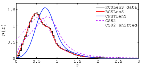
with $(a_{1},b_{1},c_{1},d_{1})=(1.50,0.32,0.20,0.46)$, as shown in van Waerbeke et al. (2013, hereafter vW13). We show this function in Fig. 1 as the blue solid line.

3.1.2 RCSLenS shear data

The RCSLenS data consists of 14 disconnected regions whose combined total area reaches 785 deg². Since photometric information is incomplete for several fields, the redshift distribution is estimated using the CFHTLenS sample augmented with near-IR and GALEX near-UV data. This new photometric sample, called CFHTLenS-VIPERS, is calibrated against  60,000 spectroscopic redshifts, as described in Coupon et al. (2015). We first apply a magnitude cut $18.0\leq\mbox{mag}_{r}\leq 24$ on the RCSLenS data, which produces a sample of 10,586,079 galaxies. The construction of the $n_{\rm RCS}(z)$ that best describes this sample is then obtained by stacking the photometric redshift PDF of the CFHTLenS-VIPERS galaxies that pass the same RCSLenS selection criteria. In addition to this magnitude cut, two modifications must be included in order to account for differences between CFHTLenS and RCSLenS:

1. The CFHTLenS limiting magnitude is approximately 1.5 mag deeper than RCSLenS. Objects in CFHTLenS-VIPERS are randomly discarded in order for the $r$-band magnitude counts to match RCSLenS counts.

2. The PDF stacking has to account for the lensfit weight, since the shear data are weighted this way. This is accomplished by measuring the relation between $r$-band magnitude and lensfit weight in RCSLenS, and applying these weights to the CFHTLenS-VIPERS galaxies based on this. We establish this relationship by binning the selected RCSLenS galaxy sample in narrow magnitude bins and calculating the average lensfit weight in each bin.

The $n_{\rm RCS}(z)$ distribution is then constructed using the CFHTLenS-VIPERS photometric redshift PDFs of galaxies in the $18.0\leq\mbox{mag}_{r}\leq 24$ magnitude range, using the magnitude-weighting relation found in (ii)- and the adjusted counts from (i). Finally, we require again FIT_CLASS=1. The source distribution is shown in Fig. 1 as the black histogram, and can be fitted by:

$$n_{\rm RCS}(z)=a_{2}\ z\ \mbox{exp}\bigg{[}\frac{-(z-b_{2})^{2}}{c_{2}^{2}}\bigg{]}+d_{2}\ z\ \mbox{exp}\bigg{[}\frac{-(z-e_{2})^{2}}{f_{2}^{2}}\bigg{]}+$$

$$g_{2}\ z\ \mbox{exp}\bigg{[}\frac{-(z-h_{2})^{2}}{i_{2}^{2}}\bigg{]}$$ (10)

where $(a_{2},b_{2},c_{2},d_{2},e_{2},f_{2},g_{2},h_{2},i_{2})$ = (3.126, -0.419, 0.979, 1.678, 0.404, 0.250, 0.400, 0.813, 0.121). This fit-function is shown in the figure as the red solid curve. The double bump was not present in the original CFHTLenS selection, and is the result of the improved photometric measurement in Coupon et al. (2015), compared to vW13. Note that this functional form differs from that used for CFHTLenS in equation 9, but that we show in Section 6.2 that this has consequence on the results, aside from providing a better fit. Once the lensfit weight are assigned, we compute the number density and shape noise of our RCSLenS sample, and obtain $\bar{n}=4.84$ gal/arcmin² and $\sigma_{\epsilon}=0.272$, respectively.

3.1.3 Map reconstruction

Table 1: Summary of the different properties of the 18 $\kappa$ maps used in this paper. The different areas listed here are the total unmasked area per field, which add up to 146.5 and 600.7 deg² for CFHTLenS and RCSLenS footprints respectively. All maps are smoothed with Gaussian filters with dispersion $\sigma$ = 4.24 arcmin. When applied, mask apodization reduces the total areas listed here to 130 deg² for CFHTLenS and 394.7 deg² for RCSLenS. See Fig. 3 for an example.

Survey	Fields	Area (deg2 )	pixel size (arcmin)
CFHTLenS	W1	63.6	1.0692
	W2	20.0	0.6018
	W3	41.5	0.8610
	W4	21.2	0.7188
RCSLenS	CDE0047	55.2	1.0
	CDE0133	27.8	1.0
	CDE0310	68.7	1.0
	CDE0357	27.7	1.0
	CDE1040	27.6	1.0
	CDE1111	67.7	1.0
	CDE1303	13.4	1.0
	CDE1514	66.0	1.0
	CDE1613	24.9	1.0
	CDE1645	24.0	1.0
	CDE2143	71.1	1.0
	CDE2329	38.9	1.0
	CDE2338	64.9	1.0
	CSP0320	22.8	1.0

The $\kappa_{\rm gal}$ maps reconstructed from the CFHTLenS data are described in details in vW13. These are based on the KS algorithm developed by Kaiser & Squires (1993), and include careful treatment of the mask and noise properties of the shear catalogue. Note that the four CFHTLenS mass maps have different areas and resolutions, which are detailed in Table 1. The maps are smoothed with a Gaussian filter of width $\sigma=4.24$ arcmin in order to suppress the effect of shot noise.

The same tools are used in the map making of the RCSLenS data, which are described in Hildebrandt (in prep.). The RCSLenS $\kappa$ maps are also smoothed with the same Gaussian filter used for CFHTLenS maps. In contrast with the CFHTLenS maps, the pixel size is uniform for all fields, exactly 1 arcmin on the side. The area of each field is calculated from the number and size of unmasked pixels, which gives a total unmasked area of 146.5 deg² for CFHTLenS and 600.7 deg² for RCSLenS. Mask apodization (see Section 4.1.2) reduces these areas to 130 deg² for CFHTLenS and 394.7 deg² for RCSLenS. This quantity is calculated differently for $\gamma_{t}$, and involves instead the ‘mosaic’ mask provided at the catalogue level. The areas are instead 125.4 and 462.6 for the two surveys.

Noise properties of these 18 $\kappa_{\rm gal}$ maps are studied by generating 100 noise realizations per field in which the orientations of the galaxies have been randomized. We also generate a series of B-mode maps by rotating the ellipticity of each galaxy by 45 degrees, via the transformation $(e_{1},e_{2})\rightarrow(-e_{2},e_{1})$ before proceeding with the KS reconstruction algorithm (see vW13 for details). The cross-correlation signal between these maps and the CMB lensing data is expected to be consistent with zero, providing an indicator for systematic biases in the maps or in the pipeline. To be clear, all these map products serve for the Fourier space and configuration space $\kappa_{\rm CMB}\times\kappa_{\rm gal}$ measurements, but not for the $\kappa_{\rm CMB}\times\gamma_{t}$ measurement, which is performed at the level of galaxy catalogue. Flat sky approximation is assumed in the reconstruction of the $\kappa_{\rm gal}$ maps, in the numerical simulations and in both cross-correlation estimators involving $\kappa_{\rm gal}$. In contrast, the $\gamma_{t}$ estimator is constructed with curved sky coordinates. Given the sizes of our fields, measurements made assuming curved or flat sky calculations are almost indistinguishable.

Figure 1: Redshift distribution of the selected RCSLenS sources (black histogram), compared to the fit function (red solid line, equation 10). Also shown are the $n(z)$ of the CFHTLenS (equation 9, blue solid line) and that of the CS82 survey (thick dashed line, magenta). The thin dashed line has been shifted by $\Delta z=0.2$.

3.2 $\kappa_{\rm CMB}$ maps

The core of our analysis makes use of the full-sky $\kappa_{\rm CMB}$ map provided in the 2015 Planck public data release (Planck Collaboration et al., 2015b). This map is reconstructed from a minimum-variance combination of the multi-frequency temperature and polarization maps recorded by the Planck microwave telescope, based on the quadratic lensing estimator of Hu & Okamoto (2002). The combination is performed on the component-separated SMICA maps (Planck Collaboration et al., 2015a), which mask the galactic plane and point sources prior to the lensing reconstruction. The public map is provided in multipole space as spherical harmonic coefficients in the range $10\leq\ell\leq 2048$, stored in a $N_{\rm side}=2048$ HEALPIX file. The map is noise-dominated, which explains why higher $\ell$-modes – or smaller scales – are not included.

We cut out the regions of the sky that overlap with the four CFHTLenS fields and the 14 RCSLenS fields, including an additional large band around each of these such that the final area of the cutout patch is four times larger. Indeed, we show in Section 4.2.1 that this larger cutout can improve the signal-to-noise ratio in the cross-correlation measurement by 10-18%. We also extract maps over these 18 regions from the 100 full-sky $\kappa_{\rm CMB}$ simulations and from the Planck lensing analysis mask map, which are provided in the data release.

Note that the removal of point sources from the CMB lensing map has an important effect on the cross-correlation signal, since these are often associated with massive clusters that contain a fair fraction of the galaxy lensing signal. To assess the importance of this effect, we make use of numerical simulations. We describe our strategy and report our results in Section 5.1.

4 The measurements

This section describes the cross-correlation measurements between CMB lensing and galaxy lensing using three distinct estimators. We first describe the $\kappa_{\rm CMB}\times\kappa_{\rm gal}$ analysis in Fourier space, which is similar in essence to the measurements from H15, LH15 and K15. Namely, the cross-correlation is obtained from the product of the two Fourier-transposed maps. We then present the first configuration-space measurements, which we achieve by measuring two-point correlation functions from $\{\kappa_{\rm CMB},\kappa_{\rm gal}\}$ and from $\{\kappa_{\rm CMB},\gamma_{t}\}$. Since the techniques involved in Fourier- and configuration-space measurements are quite different, we present these measurements in distinct sections.

4.1 Fourier analysis

In preparation for the Fourier-space analysis, it is important to properly account for a number of subtle numerical and observational effects, especially when comparing data and predictions. For instance, data re-binning, map smoothing, masking, zero-padding and apodization all affect the resulting cross-correlation measurement. There are two possible approaches to include them in the analysis: forward modelling the predictions as ‘pseudo-$C_{\ell}$’, and backward modelling the measurements to match the theoretical predictions. In both cases, what requires the most effort is the mask-induced effect, which involves the construction of a mode-mixing matrix. The backward modelling approach furthermore requires its inversion, which appears to introduce a higher level of bias (Asgari et al., in prep.); we therefore opted for the forward modelling method.

Among the three previous measurements, the analysis strategies differ considerably. H15 opted for backward modelling, and included data re-binning, map smoothing, mask apodization and a mode-mixing matrix in their pipelines. The recent measurement performed by K15 is based on the PolSpice software (Szapudi et al., 2001), which is a public code that provides a backward modelling measurement based on a completely different method from the pipeline used in H15. In contrast, LH15 concluded that given the noise levels of their measurement, only the beam smoothing had to be included in their forward modelling, and mention that mask-induced effects were only important for $\ell>7000$. Given the increased area of our measurement, new requirements on the accuracy of the predictions are more stringent, since the associated uncertainty must always be sub-dominant compared to other sources of error. We therefore decided to include a full mode-mixing matrix in the forward modelling, which serves at the same time as a preparation for next generation surveys.

4.1.1 Modelling the pseudo-$C_{\ell}$

Figure 2: Theoretical predictions for the auto-spectra ($ij=\kappa_{\rm CMB}\kappa_{\rm CMB}$ and $ij=\kappa_{\rm gal}\kappa_{\rm gal}$) and cross-spectrum ($ij=\kappa_{\rm CMB}\kappa_{\rm gal}$). These are based on RCSLenS specifications for the shape noise $\sigma_{\epsilon}$, number density $\bar{n}$ and redshift distributions $n(z)$. For CFHTLenS, the cross-spectrum is approximately a factor of two higher, due to a deeper $n(z)$.

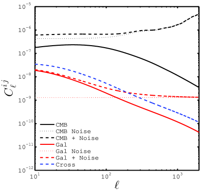
This section describes how we turn the $C_{\ell}$ predictions into pseudo-$C_{\ell}$. The main components that need to be modelled are the $C_{\ell}$ themselves, the effect of map/beam smoothing, the propagated effect of the mask and, finally, the broad binning of the measurement. The $C_{\ell}$ predictions are obtained by feeding the non-linear matter power spectrum $P(k,z)$ into equations 4 and 5. To calculate $P(k,z)$, we make use of the CAMB cosmological code (Lewis et al., 2000), based on the calibration by Takahashi et al. (2012). The source redshift distributions $n(z)$ differ between the two galaxy lensing surveys, and are obtained from the fit functions described by equations 9 and 10. Predictions for the auto- and cross-power spectra of Planck CMB lensing and RCSLenS are presented in Fig. 2, in the WMAP9 cosmology. The importance of noise in the Planck lensing map is obvious and dominates at all scales, whereas the noise in the galaxy lensing maps exceeds the signal for $\ell\gtrsim 150$.

The first part of the forward modelling concerns the map smoothing, which is obtained by multiplying the predictions by a Gaussian function whose width matches that of the Gaussian filter used in constructing the $\kappa_{\rm gal}$ maps (listed in Table 1). The CMB lensing map provided by the Planck Collaboration includes all $\ell$-modes up to 2048, hence by restricting our measurement to smaller multipoles, no modelling is necessary to account for the Planck beam.

The second part concerns the impact of observational masks. Mask-induced effects in Fourier-based analyses are discussed in detail in many papers (e.g. Feldman et al., 1994; Hivon et al., 2002; Harnois-Déraps & Pen, 2012; Asgari et al., in prep.), and can be split into three components, at least for two-point function measurements. First, they introduce an overall downward shift of power in the Fourier transform, solely due to higher number of zero elements compared to an unmasked map. This can be easily corrected for with a rescaling of the form $C_{\ell}\rightarrow C_{\ell}/\sum(M)$, where $M$ refers to the mask map, and the sum in the denominator runs over all pixels. Second, masking introduces sharp features in the observation field which, unless smoothed out by apodization, propagate in the power spectrum of the masked map and greatly enhance the measured values at high-$\ell$. The third effect of masking is to cause a coupling between the otherwise independent $\ell$-modes of the underlying $C_{\ell}^{ij}$. This comes from the fact that the cross-correlation measurement can expressed as a convolution between the cross-spectrum of the masks, $C_{\ell}^{M_{1}M_{2}}$, and the $C_{\ell}^{ij}$. Mathematically, the convolution can be described by a mode-mixing matrix, $\rm M_{\ell\ell^{\prime}}^{i}$, whose calculation is described in Appendix A. The mode-mixing matrix was ignored in LH15, hence for comparison purposes, we include it as an optional segment of our analysis.

The third and final part of the forward modelling approach consists of rebinning the modelled pseudo-$C_{\ell}$ the same way as the data. Although the original predictions are generally smooth, the mode-mixing matrix can introduce noisy features, which are made less significant with the rebinning process.

Since each of the 18 fields has a distinct mask, and since the RCSLenS and CFHTLenS have different source galaxy distributions and smoothing kernels, the 18 pseudo-$C_{\ell}$ measurements are not expected to converge to a unique predicted value. Instead, each field has its own, distinct, forward-modelled prediction, hence to combine them we must adopt the following strategy: For each field individually,

1. we measure the pseudo-$C_{\ell}^{\kappa_{\rm CMB}\kappa_{\rm gal}}$;

2. depending on whether the field belongs to RCSLenS or CFHTLenS, we select the $C_{\ell}^{\kappa_{\rm CMB}\kappa_{\rm gal}}$ prediction with the appropriate $n(z)$;

3. we apply the map smoothing kernel and, optionally, the mode-mixing matrix that correspond to this field;

4. we rebin the measurements and predictions into coarse $\ell$-bands;

5. we construct the covariance matrix (see Section 4.3 for details).

We finally combine the 18 data vectors (along with their 18 covariance matrices) into one large data vector (and one large covariance matrix) from which we can constrain cosmology. In this process, we assume that the 18 fields are generally separated well enough on the sky so that the covariance between them can be ignored. There is actually some overlap between the larger cutouts of two RCSLenS and CFHTLenS fields, but this can only have a negligible effect on the covariance. The final covariance matrix therefore consists of 18 diagonal blocks, with zeros everywhere else. Section 4.1.5 contains details about these five steps, however we must first describe step zero, which concerns the map preparation.

In the three previous $\kappa_{\rm CMB}\times\kappa_{\rm gal}$ analyses, the lensing maps were prepared and analyzed differently. Indeed, a number of choices are available with regards to mask apodization (and how this is done), zero-padding of the maps, multiplication of the $\kappa_{\rm CMB}$ and $\kappa_{\rm gal}$ masks, selecting the best sizes for the $\kappa_{\rm gal}$ smoothing kernels, etc. All of these impact the measurement, only partial justification is provided in H15, LH15 and K15 to support their choices. In this section, we seek to fill this gap and present how we optimize our analysis by comparing different pipelines, summarized in Table 2. We investigate their effects all the way down to the signal-to-noise ratio, which we present in Section 6.

4.1.2 Apodization

Mask apodization refers to the explicit smoothing of the mask, and is meant to soften the sharp transitions that occur between masked and unmasked regions. In Fourier analyses, this procedure lowers the impact of the mask on the measurement, especially for high-$\ell$ modes. It also has important effects on the mode-mixing matrix as it significantly suppresses the far off-diagonal elements, thereby making the estimator more stable (Asgari et al., in prep.). At the same time, apodization reduces the area over which the measurement is carried out, thus increasing the statistical noise. We explore this tradeoff in accuracy/precision by including it as an optional module.

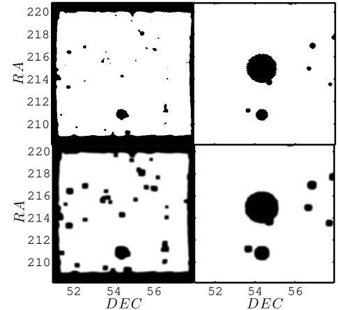
When apodization is turned on, we identify each masked pixel, set to zero all neighbouring cells separated by 5 pixels or less, and convolve the resulting mask by a Gaussian filter with a width of about 2 cells, such that the transition between zeros and ones occurs over these 5 cells. The pixels that were originally masked acquire a slight offset after this and we force them back to zero. The apodized masks are finally re-applied on the original $\kappa_{\rm gal}$ and $\kappa_{\rm CMB}$ maps by a simple multiplication. A visual example of this procedure is shown in Fig. 3, in the case of the CFHTLenS W3 field, which clearly illustrates the loss of area.

Figure 3: Mask of the CFHTLenS field W3, original (top left) and apodized with a Gaussian beam over 5 pixels (bottom left). In this case, the area drops by 10%, but the effect is more dramatic in other regions. The right panels show the Planck masks over the same region, with and without apodization.

4.1.3 Zero-padding of $\kappa_{\rm gal}$

A common practice in Fourier analyses is to zero-pad the maps, which consists of surrounding the data with a band of pixels set to zero, typically doubling the size of the data in each dimension. This technique avoids aliasing when manipulating non-periodic maps, plus it allows for an interpolation between the Fourier modes that can sometimes increase the smoothness of the measurement.

In the case of cross-correlations, the two maps are not necessarily equal in size, and one can perform the Fourier analysis by adding layers of zeros to the smaller map until it matches the size of the larger map. In our case, the Planck $\kappa_{\rm CMB}$ map covers the full sky, whereas the 18 $\kappa_{\rm gal}$ maps are scattered all around, with sizes varying between 14 and 78 deg². If we were to follow the three previous analysis strategies, we would carve out these exact 18 footprints from the Planck lensing map. In fact, we have the freedom to choose $\kappa_{\rm CMB}$ maps of any size, and there is a potential gain in signal-to-noise that can be achieved by cutting out larger maps. Indeed, a non-zero correlation length implies that regions of $\kappa_{\rm CMB}$ outside the survey footprint are correlated with regions of $\kappa_{\rm gal}$ inside of it. This is best explained with a simple toy example.

We are interested in cross-correlating two maps – in our case $\kappa_{\rm CMB}$ and $\kappa_{\rm gal}$ – which we label $M_{1}(\boldsymbol{\theta})$ and $M_{2}(\boldsymbol{\theta})$ to keep the discussion general. For simplicity, we also neglect small scales cutouts from the observed maps in this example, and only consider the large scale footprints. Let us suppose that $M_{1}$ extends over a large region, $A$, while $M_{2}$ is measured only over a smaller region, $B$, with $B\subseteq A$. If we decided to measure the cross-correlation only over the part of the sky that perfectly overlaps (region $B$), we would reject any area from $M_{1}$ that is outside $B$, and our pseudo-$C_{\ell}$ estimator would be written as:

$$\langle M_{1,\ell}M_{2,\ell}^{*}\rangle_{B}={\rm Re}\langle\!\!\int\!\!\!\!\int_{B}M_{1}(\boldsymbol{\theta})M_{2}(\boldsymbol{\theta}^{\prime})e^{i\boldsymbol{\ell}(\boldsymbol{\theta}-\boldsymbol{\theta}^{\prime})}\mbox{d}\boldsymbol{\theta}\mbox{d}\boldsymbol{\theta}^{\prime}\rangle$$ (11)

The square brackets here refer to the polar integration, and the integration is carried solely over region $B$. We refer to this as the ‘adjusted’ maps estimator. Alternatively, we could decide to measure the cross-correlation over all the available data, i.e.

$$\langle M_{1,\ell}M_{2,\ell}^{*}\rangle_{A,B}={\rm Re}\langle\!\!\int_{A}\!\!\int_{B}M_{1}(\boldsymbol{\theta})M_{2}(\boldsymbol{\theta}^{\prime})e^{i\boldsymbol{\ell}(\boldsymbol{\theta}-\boldsymbol{\theta}^{\prime})}\mbox{d}\boldsymbol{\theta}\mbox{d}\boldsymbol{\theta}^{\prime}\rangle$$ (12)

where now the two integrals run over different regions $A$ and $B$. As mentioned before, the numerical implementation of this measurement involves zero-padding $M_{2}$ such that it matches $M_{1}$ in size. Then both integrals can be carried over region $A$, and we refer to this as the ‘large’ maps estimator.

In order to find out whether there is a difference between these two measurements, we subtract equation 11 from equation 12:

$$\langle M_{1,\ell}M_{2,\ell}^{*}\rangle_{A,B}-\langle M_{1,\ell}M_{2,\ell}^{*}\rangle_{B}={\rm Re}\langle\!\!\int_{A-B}\!\!\!\!M_{1}(\boldsymbol{\theta})\!\!\int_{B}\!\!M_{2}(\boldsymbol{\theta}^{\prime})e^{i\boldsymbol{\ell}(\boldsymbol{\theta}-\boldsymbol{\theta}^{\prime})}\mbox{d}\boldsymbol{\theta}\mbox{d}\boldsymbol{\theta}^{\prime}\rangle$$ (13)

This is effectively computing the correlation between $M_{2}$ inside region $B$ with $M_{1}$ outside region $B$. When the two maps are uncorrelated, this obviously vanishes. However, any correlation that exists between the two maps would make this subtraction non-zero, provided that the correlation length exceeds one pixel. When we replace $M_{1}$ and $M_{2}$ by $\kappa_{\rm CMB}$ and $\kappa_{\rm gal}$ and realize that the correlation length predicted by equation 7 extends at least to one degree, it becomes clear that the ‘large’ maps estimator should have a better signal-to-noise, although the level of improvement is not obvious.

Technically, only the $\kappa_{\rm gal}$ map is zero-padded in this procedure – on the contrary, the area selected from the $\kappa_{\rm CMB}$ map is larger, thereby adding a large amount of non-zero elements. Failing to find a better name to describe this procedure, we still refer to it as ‘zero-padding’, with the understanding that it is not an accurate description of what is going. This zero-padding strategy has not been used in the previous CMB lensing-galaxy lensing analyses, and was not even an option for the ACT/CS82 and SPT/DES-SV data since their footprints exactly match. To quantify the actual gain that it provides, we perform our analysis on both adjusted $\kappa_{\rm CMB}$ maps (exact $\kappa_{\rm gal}$ footprints) and larger maps (4 times the area of the $\kappa_{\rm gal}$ footprints, zero-padding the $\kappa_{\rm gal}$ maps), and propagate the impact on the cosmological constraints.

4.1.4 Mask Combination

Table 2: Different forward modelling pipelines P examined in this paper to carry out the pseudo-$C_{\ell}$ measurement. LH15 used pipeline P5, while H15 and K15 used two different backward modelling versions of pipeline P5. As described in Section 4.1.3, what we mean by ‘zero-padding’ differs from the traditional usage, as it refers to the analysis of $\kappa_{\rm CMB}$ cutout maps that are 4 times larger than the $\kappa_{\rm gal}$ footprints. Only the latter is zero-padded, whereas we keep the full $\kappa_{\rm CMB}$ values in the padded region. ‘Joint mask’ means multiplying the masks from both maps, and re-applying the result on both maps.

Pipeline	apodization	zero-pad	joint mask
P1	no	no	no
P2	yes	no	no
P3	no	yes	no
P4	yes	yes	no
P5	yes	no	yes

The last step in the map preparation concerns the method by which the masks (from the $\kappa_{\rm CMB}$ and $\kappa_{\rm gal}$ maps) are incorporated in the measurement. Despite the potential gain in signal-to-noise ratio that can be accessed by following the method described in Section 4.1.3, previous studies by H15, LH15 and K15 have opted for a strategy based on equation 11 according to which the analyses require ‘adjusted’ maps. Moreover, they constructed a ‘joint mask’ from the product of both masks, and applied it back on all their maps. As briefly mentioned at the end of Section 3.2, combining masks in this way has severe consequences on the cross-correlation signal, since the point sources that are masked in $\kappa_{\rm CMB}$ correspond to regions of high signal in $\kappa_{\rm gal}$. There is therefore a strong correlation between the $\kappa_{\rm CMB}$ mask and the $\kappa_{\rm gal}$ maps, which biases the measurement unless properly accounted for. We explore this approach as well, mainly for comparison purposes, but we otherwise treat both masks separately.

To organize our numerous measurement strategies, we refer to a particular choice of apodization, zero-padding and joint-masking as a ‘pipeline’. We consider five different pseudo-$C_{\ell}$ pipelines, which are labelled P1-P5 and detailed in Table 2. From our numerical simulations presented in Section 5.2, we find that only P5 significantly suffers from mask-induced effects, hence our results do not include the mode-mixing calculations unless explicitly specified.

4.1.5 Measuring the pseudo-$C_{\ell}$

Figure 4: Area-weighted average of the cross-spectrum between the $\kappa_{\rm CMB}$ maps from the Planck 2015 data release and the $\kappa_{\rm gal}$ maps from the RCSLenS (left) and CFHTLenS (right). These pseudo-$C_{\ell}$ measurements are carried out with pipeline P1, which has the highest signal-to-noise ratio; we compare the other pipelines summarized in Table 2 in Fig. 18. In both panels, the black error bars are obtained from the cross-correlation between the 100 CMB lensing maps and the E-mode $\kappa_{\rm gal}$ maps, while the blue errors show the analytical Gaussian predictions (equation 23). The correlation between the points is negligible. The three null tests shown here are CMBLenS simulations x RCSLenS data (E- and B-modes), and CMBLenS data x RCSLenS random catalogues, as described in Section 5.4.

For each pipeline listed in Table 2, we measure the pseudo-$C_{\ell}$ in the following way. We first compute the amount of unmasked area common to both maps for each field $i$, $\sum(M^{i})$, in preparation for the $C_{\ell}\rightarrow C_{\ell}/\sum(M)$ rescaling mentioned in Section 4.1.1. We then Fourier transform the galaxy lensing and CMB lensing maps, complex-multiply the results and reject the imaginary part. Denoting observed quantities with a ‘hat’, this operation estimates $\hat{C}^{\kappa_{\rm CMB}\kappa_{\rm gal},i}_{\boldsymbol{\ell}}$. A finely-binned cross-spectrum is then found by angle-averaging this quantity in annuli of width $\Delta\ell^{i}=2\pi/\theta_{\rm max}^{i}$, where $\theta_{\rm max}^{i}$ is the angular size of the largest dimension for the field $i$. Noting that the maps are not strictly square, the density of the Fourier modes is slightly anisotropic, which our calculation takes into account. So far this measurement knows nothing about masks: it treats zero-valued pixels as any other pixels, and the resulting $\hat{C}^{\kappa_{\rm CMB}\kappa_{\rm gal},i}_{\boldsymbol{\ell}}$ are highly suppressed for heavily masked fields. We therefore rescale the results as $\hat{C}^{\kappa_{\rm CMB}\kappa_{\rm gal},i}_{\ell}\rightarrow\hat{C}^{\kappa_{\rm CMB}\kappa_{\rm gal},i}_{\ell}/\sum(M^{i})$ to correct for this.

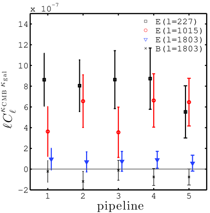
Following LH15, we next calculate the average of the measurements inside five coarse bins that are linearly spaced in the range $\ell=\{30,2000\}$, with width $\Delta\ell_{c}=394$ and centred on $\ell_{c}$ = (227, 621, 1015, 1409, 1803). We repeat this pseudo-$C_{\ell}$ measurement on the 18 fields and with methods P1-P5 for the $\kappa_{\rm CMB}\times\kappa_{\rm gal}$ data, as well as for a number of supplementary maps that serve for null tests and error estimates that we detail in Section 5.4.

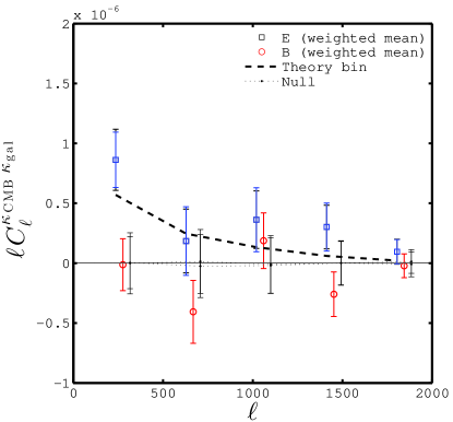
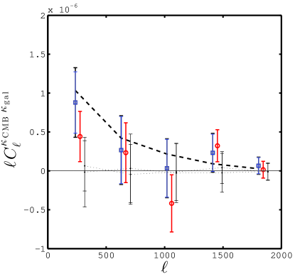
We present our cross-correlation measurements in Fig. 4 for RCSLenS (left) and CFHTLenS (right). We only show here the results from pipeline P1, but include P1-P5 in Appendix B. In both panels, the thick black squares represent the $\hat{C}_{\ell}^{\kappa_{\rm CMB}\kappa_{\rm gal}}$ measurement, while the thick red circles and the black points are null tests described in Section 5.4. The thick dashed lines represent the pseudo-${C}_{\ell}^{\kappa_{\rm CMB}\kappa_{\rm gal}}$ predictions in the WMAP9 cosmology. The gain in precision is clearly seen in RCSLenS measurements compared to CFHTLenS and is purely due to the larger area coverage. The predicted $\ell$-dependence of the signal becomes apparent, although its shape is poorly resolved. However, one of the main advantages of the Fourier analysis over the two configuration-space analyses is that the data points shown here are very weakly correlated. The error bars are estimated by combining 100 Planck lensing simulations with the measured $\kappa_{\rm gal}$, as detailed in Section 4.3.

4.2 Configuration-space analysis

The main advantage of the configuration-space measurement is that the effect of masking is much milder than in Fourier space. It affects the reconstruction of the $\kappa_{\rm gal}$ map, since it is the shear map that are masked. For the $\gamma_{t}$ estimator, it simply reduces the observation area. In addition, there is no need for mask apodization nor mode-mixing matrices, which makes the analysis much simpler. The measurements from all 14 RCSLenS fields are expected to converge to the same value, and the same can be said for the four CFHTLenS fields. Only the $n(z)$ and the map smoothing differ between both surveys, which still needs to be modelled. The combination of the different fields become a simple weighted mean over the individual measurements. In fact, forward and backward modelling become more directly connected; we choose the former such as to be consistent with the Fourier analysis. However, these configuration-space analyses require a slightly different preparation of the data.

4.2.1 Data preparation

Although this is not a requirement, we choose to down-weight the noise of the $\kappa_{\rm CMB}$ map by applying a Wiener filter:

$$\kappa^{\rm CMB,WF}_{\ell m}=\frac{C^{\kappa_{\rm CMB,th}}_{\ell}}{C^{\kappa_{\rm CMB,th}}_{\ell}+N_{\rm CMB}}\ \kappa_{\ell m}^{\rm CMB}$$ (14)

where $C^{\kappa_{\rm CMB,th}}_{\ell}$ is the best-fit auto-power spectrum of the lensing map, and $N_{\rm CMB}$ is the total (instrumental + statistical) noise spectrum, both provided in the public Planck data release. This filtering is accomplished on the full-sky map (i.e. before carving out the field footprints) and therefore this part of the analysis – and only this part – uses spherical harmonic transforms as opposed to Cartesian Fourier transforms. We have checked different filtering procedures, as well as no filtering at all, and the significance of the measured cross-correlation signal is not strongly affected.

As mentioned above, apodization is no longer necessary, however the zero-padding technique presented in Section 4.1.3 can provide advantages here as well. To illustrate this, let us re-examine the toy example where maps $M_{1}$ and $M_{2}$ are measured over regions $A$ and $B$, respectively. From a configuration-space perspective, the difference between the estimators for the ‘large’ and the ‘adjusted’ maps (equation 13) becomes:

$$\langle M_{1}(\theta+\Delta\theta)M_{2}(\theta)\rangle_{A,B}-\langle M_{1}(\theta+\Delta\theta)M_{2}(\theta)\rangle_{B}$$ (15)

where $\theta\in B$ in both terms, $(\theta+\Delta\theta)\in A$ in the first term, but $(\theta+\Delta\theta)\in B$ in the second term. After the subtraction, what is left is a contribution from $\theta\in B$ while $(\theta+\Delta\theta)\notin B$, i.e. the correlation between $M_{1}$ and the part of $M_{2}$ that is outside region $B$. Again, with $M_{1}\rightarrow\kappa_{\rm CMB}$, $M_{2}\rightarrow\kappa_{\rm gal}$ or $\gamma_{t}$, and recalling that the correlation length of these two estimators stretches beyond a degree (from equations 7 and 8, shown in Fig. 5), it is possible to improve the analysis by analyzing the ‘large’ $\kappa_{\rm CMB}$ maps as opposed to the ‘adjusted’ maps. We carried out the measurements on both types of maps and found that the signal-to-noise ratio (SNR, see Section 6.1) is improved by 10-18% in the large maps, compared to the adjusted maps. We therefore opted for the former in our analysis.

After examination of the predictions for our two configuration-space cross-correlation estimators, it appears that the cross-correlation signal extends to 3 degrees, but not much beyond. We therefore include a region that is 3 degrees thick on each side of the CFHTLenS fields, and extend this to 4 degrees for the RCSLenS. Because the largest measured angular bin from RCSLenS (CFHTLenS) is 3 (2) degrees, no information is lost by not using a larger padding. We otherwise proceed exactly as for the map preparation in the Fourier analysis: we surround the $\kappa_{\rm gal}$ maps with layers of zero elements until their size matches that of the $\kappa_{\rm CMB}$ maps. This is even more direct for the $\gamma_{t}$ estimator, which is computed directly from the galaxy catalogue: we simply feed the ‘adjusted’ or the ‘large’ $\kappa_{\rm CMB}$ maps in the estimator. More details about this are provided in the next section.

4.2.2 The estimators

Figure 5: Configuration-space cross-correlation between the Planck 2015 and RCSLenS lensing data, plotted against WMAP9 predictions described by equations 7 and 8. The error bars are computed from 100 CMB lensing simulations, which confirm that the points are highly correlated. The Planck CMB maps have been Wiener filtered to reduce the noise levels. Black squares show Planck cross E-modes, red circles show Planck cross B-modes, as in Fig. 4.

The configuration-space $\kappa_{\rm CMB}\times\kappa_{\rm gal}$ estimator of the two-point correlation function is computed as follows:

$$\xi^{\kappa_{\rm CMB}\kappa_{\rm gal}}(\vartheta)=\frac{\sum_{ij}\kappa_{\rm CMB}^{i}\kappa_{\rm gal}^{j}\Delta_{ij}(\vartheta)}{\sum_{ij}\Delta_{ij}(\vartheta)}.$$ (16)

The sum runs over all pixels $i$ at positions $\boldsymbol{\theta}_{i}$ on the $\kappa_{\rm CMB}$ map and pixels $j$ on the corresponding $\kappa_{\rm gal}$ map. The term $\Delta^{ij}$ controls the binning, which is organized in 6 broad bins of width $\Delta$ = 30 arcmin each (we use 4 bins for CFHTLenS given the higher noise levels) with:

$$\Delta^{ij}(\vartheta)=\begin{cases}1{\rm,if}\left|{\boldsymbol{\theta}}_{i}-{\boldsymbol{\theta}}_{j}\right|<\vartheta\pm\frac{\Delta}{2}\\ 0{\rm,otherwise}\end{cases}$$ (17)

The sum is performed with a k-d tree algorithm to speed up the computation by only checking pairs that are not separated more than the largest bin.

The second configuration-space estimator that we use is this paper is a generalization of the galaxy-galaxy lensing estimator, which is typically extracted by stacking the tangential shear signal from background galaxies around a discrete set of foreground objects, usually foreground galaxies. For the $\kappa_{\rm CMB}\times\gamma_{t}$ estimator, we perform a similar stacking, but this time we stack on all pixel positions instead of foreground galaxies, and weight the sum by the pixel values. The $\kappa_{\rm CMB}\times\gamma_{t}$ estimator is given by:

$$\xi^{\kappa_{\rm CMB}\gamma_{t}}(\vartheta)=\frac{\sum_{ij}\kappa_{\rm CMB}^{i}e_{t}^{ij}w^{j}\Delta_{ij}(\vartheta)}{\sum_{ij}w^{j}\Delta_{ij}(\vartheta)}\frac{1}{1+K(\vartheta)}\,$$ (18)

where $\Delta_{ij}(\vartheta)$ is the binning operator described by equation 17. In this case, the sum runs over all pixel $i$ in the $\kappa_{\rm CMB}$ map, and all galaxies $j$ in the CFHTLenS or RCSLenS survey. Here $e_{t}^{ij}$ is the tangential component of the ellipticity of a galaxy $j$ (at position ${\boldsymbol{\theta}}_{j}$) with respect to the pixel $i$ in $\kappa_{\rm CMB}$ (at position ${\boldsymbol{\theta}}_{i}$). The B-mode signal is extracted by replacing $e_{t}^{ij}$ by the cross-shear $e_{x}^{ij}$ in the above expression. For technical details about the definition of the ellipticity components $e_{t}$ and $e_{x}$, see for example Viola et al. (2015). The quality of the shape measurement is determined by the lensfit weight (Miller et al., 2013) and is denoted by $w^{j}$. The trailing factor $(1+K(\vartheta))^{-1}$ accounts for the multiplicative bias correction:

$$\frac{1}{1+K(\vartheta)}=\frac{\sum_{ij}w^{j}\Delta_{ij}(\vartheta)}{\sum_{ij}w^{j}(1+m^{j})\Delta_{ij}(\vartheta)}\ .$$ (19)

It is straightforward to extend this estimator to other types of cross-correlation measurements, simply by replacing $\kappa_{\rm CMB}$ by another map (for an application on tSZ $\times\gamma_{t}$, see Hojjati et al., in prep.).

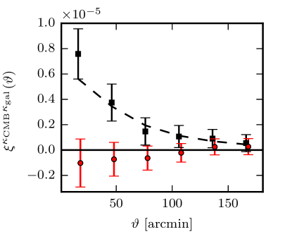
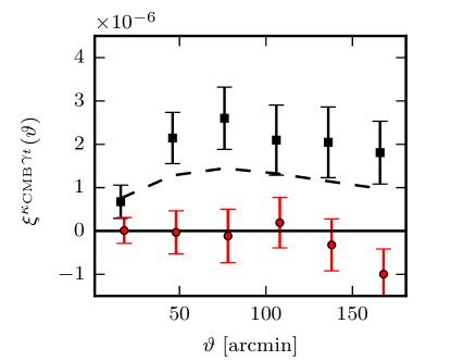
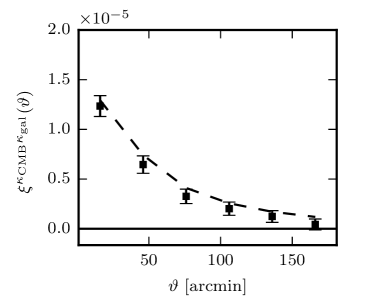
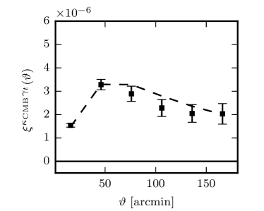
We present in Fig. 5 the results from these two measurements on the RCSLenS fields, against theoretical predictions from the WMAP9 cosmology. The data and predictions are in good agreement for both the $\xi^{\kappa_{\rm CMB}\kappa_{gal}}$ and $\xi^{\kappa_{\rm CMB}\gamma_{t}}$ measurements. The later prefers slightly higher values than WMAP9, but this preference is weak, especially when considering the fact that points here are highly correlated.

4.3 Covariance Estimation

We describe in this section our strategy to construct an accurate covariance matrix, which, for our Fourier analysis, largely follows the methods of H15, LH15 and K15.

4.3.1 Fourier-space covariance

The uncertainty about the measurement $\hat{C}^{\kappa_{\rm CMB}\kappa_{\rm gal}}_{\ell}$ is evaluated from the expression:

$$\widehat{\rm Cov}^{\kappa_{\rm CMB}\kappa_{\rm gal}}_{\ell\ell^{\prime}}=\langle\Delta\hat{C}^{\kappa_{\rm CMB}\kappa_{\rm gal}}_{\ell}\Delta\hat{C}^{\kappa_{\rm CMB}\kappa_{\rm gal}}_{\ell^{\prime}}\rangle,$$ (20)

where again the ‘hat’ symbols refer to ‘observed’ quantities. Knowing that the noise $N_{\rm CMB}$ is much larger than the signal $\kappa_{\rm CMB}$ (see Planck Collaboration et al., 2015b, and Fig. 2), we can write:

$$\widehat{\rm Cov}^{\kappa_{\rm CMB}\kappa_{\rm gal}}_{\ell\ell^{\prime}}\simeq\langle\Delta\hat{C}^{N_{\rm CMB}\kappa_{\rm gal}}_{\ell}\Delta\hat{C}^{N_{\rm CMB}\kappa_{\rm gal}}_{\ell^{\prime}}\rangle.$$ (21)

From this, it follows that the complete covariance can be captured by cross-correlating the observed $\kappa_{\rm gal}$ maps with CMB lensing noise maps, or alternatively with CMB lensing simulations, from which only the noise component will be measured. For this purpose, we use the 100 simulations provided by the Planck release. The covariance extracted from these 100 cross-correlation measurements serves as our estimation of the error about $\hat{C}^{\kappa_{\rm CMB}\kappa_{\rm gal}}_{\ell}$.

Note that the map masking and smoothing is already included this estimate (and in equation 21), therefore the error extracted this way is exactly what is needed for the forward modelling approach. In a backward modelling approach however, one would need to deconvolve the mode-mixing matrix from this estimate by solving:

$$\widehat{\rm Cov}^{\kappa_{\rm CMB}\kappa_{\rm gal}}={\rm M}{\rm Cov}^{\kappa_{\rm CMB}\kappa_{\rm gal}}{\rm M}^{T}.$$ (22)

Since the scales involved are mostly in the linear regime, it is possible to verify our error estimate against the Gaussian prediction:

$$\widehat{\rm Cov}^{\kappa_{\rm CMB}\kappa_{\rm gal}}_{\ell\ell^{\prime},G}=\frac{\delta_{\ell\ell^{\prime}}}{f_{\rm sky}(2\ell+1)\Delta\ell}\bigg{(}\hat{C}^{\kappa_{\rm CMB}}_{\ell}\hat{C}^{\kappa_{\rm gal}}_{\ell}+\bigg{[}\hat{C}^{\kappa_{\rm CMB}\kappa_{\rm gal}}_{\ell}\bigg{]}^{2}\bigg{)}.$$ (23)

In the above expression, $\Delta\ell$ is the bin width, $\delta_{\ell\ell^{\prime}}$ is the Kronecker delta function, and $f_{\rm sky}$ is the sky fraction commonly covered by both fields, including masking and apodization (when applicable). By inserting the observed auto-spectra $\hat{C}^{\kappa_{\rm CMB}}_{\ell}$ and $\hat{C}^{\kappa_{\rm gal}}_{\ell}$ as opposed to the theoretical values, these Gaussian predictions naturally take into account the statistical noise, the effect of masks and smoothing. The cross-spectrum term $\hat{C}^{\kappa_{\rm CMB}\kappa_{\rm gal}}_{\ell}$ can be replaced by the theoretical value $C^{\kappa_{\rm CMB}\kappa_{\rm gal}}_{\ell}$ since the effects of masking are much lower and the two noise contributions are uncorrelated. The different terms entering equation 23 are presented in Fig. 6. We see therein that in the absence of noise, the cross-term is an order 10-50% correction to the leading term, whereas it is currently a negligible $<10\%$ correction on the error. In this Gaussian calculation, we define the observed convergence map power spectrum as:

$$\hat{C}^{\kappa_{\rm gal}}_{\ell}=C^{\kappa_{\rm gal,th}}_{\ell}+\frac{\sigma_{\epsilon}^{2}}{\bar{n}},$$ (24)

where the galaxy intrinsic shape dispersion is given by $\sigma_{\epsilon}$ = 0.278 and 0.272 for the CFHTLenS and RCSLenS respectively, and the mean number density by $\bar{n}$ = 8.30 and 4.25 gal/arcmin² (see Section 3.1). Since the covariance scales linearly with the auto-spectra and with the inverse of the sky coverage, the error bars on the RCSLenS measurements are $\sim\sqrt{2}$ smaller than those from CFHTLenS (the expected signal is about twice smaller due to the shallower $n(z)$, but benefits from four times the area).

Figure 6: Theoretical predictions for the two terms that enter the Gaussian error predictions of equation 23, shown in the WMAP9 cosmology for the RCSLenS survey. The black solid (dashed) line corresponds to the first term – $\hat{C}^{\kappa_{\rm CMB}}_{\ell}\hat{C}^{\kappa_{\rm gal}}_{\ell}$ – without (with) the noise contribution. The blue line represents the second term – $\left[\hat{C}^{\kappa_{\rm CMB}\kappa_{\rm gal}}_{\ell}\right]^{2}$ – which is always subdominant. The noise-free error for CFHTLenS is about twice that of RCSLenS given its higher signal, but that difference is reduced when noise is included in the predictions.

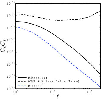
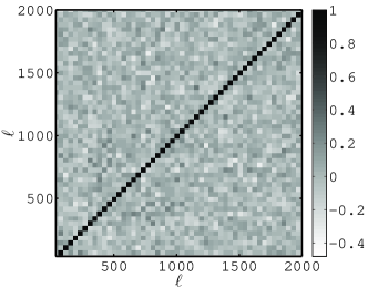
The Gaussian predictions are shown as the blue error bars in Fig. 4, whereas the error extracted from the 100 CMB lensing simulations is shown in black. Both error estimates are in close agreement in all pipelines, often better than 10%. Following H15, LH15 and K15, we use the latter in our error analysis, which are computed for each field separately. These contain non-zero off-diagonal elements that play a minimal role, as seen in Fig. 7 for RCSLenS field CSP0320. As expected from the Gaussian predictions and shown here, the correlations between different Fourier modes are always negligible. The off-diagonal elements are nevertheless important carriers of noise properties. As shown in Taylor et al. (2013), the fractional noise in a covariance matrix of $N_{d}^{2}$ elements, estimated from $N_{s}$ simulations, can be estimated as $\sqrt{2/(N_{s}-N_{d}-2)}$. In a one-parameter measurement – in our case the amplitude of the cross-correlation signal – this error propagates through to an extra covariance term on the parameter, which inflates the covariance by $(1+1)/(N_{s}-N_{d})[1+2/(N_{s}-N_{d})]=0.022$ (Taylor & Joachimi, 2014). Because this 2% effect is small compared to the other error terms, we do not include it here. The noise in the covariance matrix has a second effect: it produces an error on the error, which can often be catastrophic. Given our numbers of simulations and data points, the fractional error on our error reaches $\epsilon=\sqrt{2/N_{s}+2(N_{d}/N_{s}^{2})}=14.5\%$. Since it is non-negligible, we decided to be conservative and modify our final uncertainty to include the upper $1\sigma$ limit (details can be found in Section 6.1). Note that the three previous paper omitted to include this extra error, hence care should be taken when comparing results.

4.3.2 Configuration-space covariance

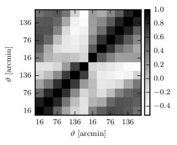
We estimate the covariance about our configuration-space estimators in a similar way, i.e. from 100 $\kappa_{\rm CMB}\times\kappa_{\rm gal}$ measurements carried out with the Planck lensing simulations. The diagonal elements are used to estimate the error bars in Fig. 4, while the cross-correlation coefficients are shown in Fig. 8 for the joint $\{\xi^{\kappa_{\rm CMB}\kappa_{\rm gal}},\xi^{\kappa_{\rm CMB}\gamma_{t}}\}$ data vector. There is a high level of correlation between pairs of data points within the same estimator (lower left and upper right blocks), while pairs that come from both estimators (off-diagonal blocks) are subject to a strong correlation or anti-correlation, depending on the angular bins they belong to. This is expected as the different points measure mostly the same matter structures, and the two configuration-space estimators probe slightly different scales.

Figure 7: Cross-correlation coefficient matrix measured from the RCSLenS field CSP0320, defined as $r_{ij}=\mbox{Cov}_{ij}/\sqrt{\mbox{Cov}_{ii}\mbox{Cov}_{jj}}$. Within noise, this is consistent with the Gaussian diagonal predictions. Measurements of $r_{ij}$ made on other fields are very similar to this one.

Figure 8: Cross-correlation coefficient matrix about the configuration-space estimators, measured from all RCSLenS fields. The first six bins along each axis represent the correlation about $\xi^{\kappa_{\rm CMB}\kappa_{\rm gal}}$, while the last six show $\xi^{\kappa_{\rm CMB}\gamma_{t}}$.

5 Validation

This section describes a series of tests performed first on the analysis pipelines, then on the data products, that are meant to validate our results.

5.1 Numerical simulations

Figure 9: (top left:) One of the 50 simulated $\kappa_{\rm gal}$ maps from the SLICS series, shown with full $6000^{2}$ pixel resolution and for $z_{s}=0.58$. In our validation pipeline, the map is first convolved with a 6 arcmin Gaussian beam to mimic the resolution of the data maps (top middle panel), then we apply the W3 mask (top right). The three bottom panels show the same procedure, this time for the $\kappa_{\rm CMB}$ map as $z=1080$, using the mask from the Planck lensing analysis that covers the W3 footprint.

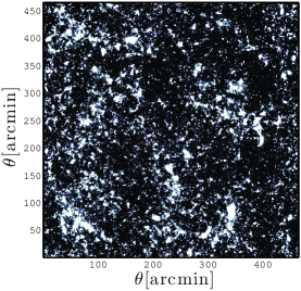
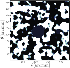
We verify our Fourier pipelines against numerical simulations, for which the cosmology is known, and the observational mask and smoothing can be switched on and off. This way, it is possible to validate each segment of our forward modelling procedure. The map reconstruction algorithm has been thoroughly tested in vW13, and it is actually the cross-correlation measurement itself that is investigated.

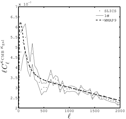
For this purpose, we use 100 lines-of-sights (LOS) from the SLICS-LE suite described in Harnois-Déraps & van Waerbeke (2015). These are dark matter only simulations that were produced from the public CUBEP³M $N$-body code (Harnois-Déraps et al., 2013), based on the WMAP9 cosmology. In the original SLICS-LE suite, each light cone is ray-traced through a series of 18 mass planes in the redshift range ${\{0,3\}}$, covering 60 deg² with a resolution of $6000^{2}$ pixels. We extend the light cones to the surface of last scattering at $z_{*}$ by filling the high-redshift region with 10 mass planes separated by 517 $h^{-1}$Mpc. In order to cover a large opening angle at the high redshift end, we opted for mass planes that are 1034$h^{-1}$Mpc on the side (exactly twice the separation distance), such that the full map can be calculated by collapsing the density field from exactly one half the simulation volume. Aside from this change in box size – the SLICS are 505$h^{-1}$Mpc on a side – the cosmology and the number of simulation elements are unchanged.

Since this high-redshift extension of the SLICS contributes only minimally in the final cross-correlation measurement, there is no need to accurately resolve the non-linear structure therein. Therefore we use a numerical solver solely based on linear perturbation theory to create mass maps at the 10 prescribed redshifts: $z_{\rm high}$ = 3.498, 4.544, 5.993, 8.086, 11.27, 16.49, 25.90, 45.63, 98.89 and 346.6. As these maps are noisy due to the discreteness of the particles, we convolve these 10 maps with a beam very close to the actual smoothing scale of the $\kappa_{\rm gal}$ maps. Note that the central purpose of these simulations is to validate the signal pipelines, not to estimate the uncertainty. As such, there is no need to create more than one of these $z>3$ extensions. Instead, we graft this single high-redshift section to 100 independent LOS, and ray-trace the full light cones up to $z_{*}$ in the Born and flat sky approximations.

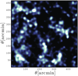
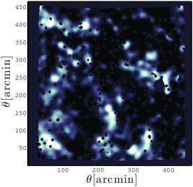
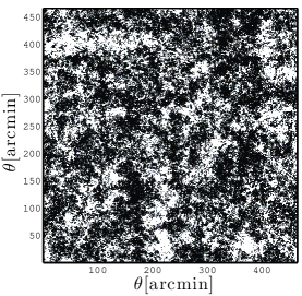
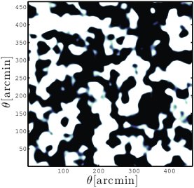
To reproduce the measurement under investigation, we include one simplification, which is to assume that all galaxy sources are located on a single redshift plane at $z_{s}=0.58$. This choice of $n(z)$ is simpler than adopting a broader distribution, yet sufficient to validate our pipelines. We then convolve both the simulated $\kappa_{\rm CMB}$ and $\kappa_{\rm gal}$ maps with a 6 arcmin beam and recover a smoothing scale comparable to that present in the data. After this smoothing, there is no need to keep the full resolution of the simulation maps, hence we lower the pixel count to approximately match that of the observations. Finally, we apply the actual observation masks. For testing purposes, we use the W3 footprint, which falls nicely within one 60 deg² simulated LOS, but we verified that our results hold for other fields. This procedure is shown in the top three panels of Fig. 9 for $\kappa_{\rm gal}$, and in the three bottom panels for $\kappa_{\rm CMB}$.

5.2 Verification of Fourier pipelines

We next proceed with the cross-spectrum analysis of these mock observations, presented in Figs. 10 and 11. We first verify the agreement between the cross-correlation predictions and the unmasked, un-smoothed simulated maps, such as those presented in the left-most panels of Figure 9. This agreement is well established in Fig. 10 where the theory falls well within the $1\sigma$ region of the simulations at all relevant scales. Smoothing is then applied on the $\kappa$ maps and the resulting cross-spectrum is shown as black open circles in the three panels of Fig. 11 (labelled $\kappa_{\rm CMB}\times\kappa_{\rm gal}$ in the legend). This serves as our reference measurement for the mask pipeline comparisons, hence we replicate these results in all panels. We do not show the smoothed predictions to avoid overcrowding the figures, but the match is as good as that of Fig. 10.

Figure 10: Cross-spectrum between the simulated $\kappa_{\rm gal}$ and $\kappa_{\rm CMB}$ maps averaged over 50 LOS. One such pair is presented in the top and bottom left panels of Fig. 9. No mask nor smoothing are applied yet. The black symbols show the simulations results, the thin lines represent the error on the mean ($1\sigma$-scatter/$\sqrt{50}$, which overlaps nicely with the input WMAP9 cosmology (dashed line).

Figure 11: Cross-spectrum between simulated $\kappa_{\rm gal}$ and $\kappa_{\rm CMB}$ maps, analyzed with different pipelines. In all panels, the black symbols show the ‘true’ signal, with no mask applied. The thin lines represent the error on the mean. In the top panel, the red and blue symbols show the effect of applying the W3 mask on either $\kappa_{\rm gal}$ or $\kappa_{\rm CMB}$, but not on both. The middle panel shows the pseudo-$C_{\ell}$ pipeline P1 (blue), and a version of P1 in which the highest peaks from $\kappa_{\rm gal}$ were deliberately masked from $\kappa_{\rm CMB}$ (red). The bottom panel compares P1, P5 and the pseudo-$C_{\ell}$ forward model corresponding to P5, labelled ‘PCL’.

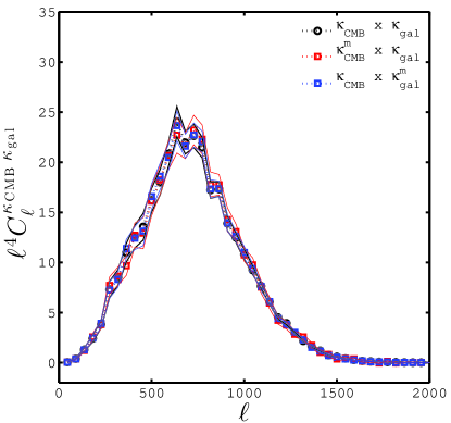
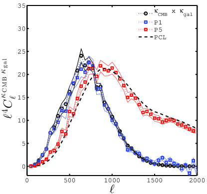
In the top panel of Fig. 11, we systematically investigate the effect of masking on these simulations. First, we compute the cross-spectrum between the unmasked $\kappa_{\rm gal}$ and masked $\kappa_{\rm CMB}$ maps (shown in red, labelled $\kappa_{\rm CMB}^{m}\times\kappa_{\rm gal}$) and between the unmasked $\kappa_{\rm CMB}$ and masked $\kappa_{\rm gal}$ maps (shown in blue, labelled $\kappa_{\rm CMB}\times\kappa_{\rm gal}^{m}$). The results are rescaled by $1/\sum(M)$, according to the discussion in Section 4.1.5. The agreement between the mean value from these two measurements and the unmasked case (black) demonstrates that these two estimators are unbiased.

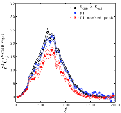
We next consider the case where both maps are masked, each with their own respective masks, thereby reproducing the pseudo-$C_{\ell}$ analysis with pipeline P1. The results are shown with the blue symbols in the central panel, which also trace faithfully the predictions up to $\ell\sim 2000$. We reproduce the same level of agreement with pipelines P2-4. There are slight undershoots and overshoots visible at $\ell\sim 600$ and $1500$ respectively, which comes from chance alignment of similar structures in the two masks or from data-mask interaction. Ignoring the mode-mixing matrix (described in Appendix A) is therefore equivalent to modelling the blue symbols with a theoretical curve passing through the black region, which is accurate in this case.

One interesting conclusion we can draw from this calculation is that if one of the maps has no mask and if the other mask does not correlate with the maps, then the pseudo-$C_{\ell}^{\kappa_{\rm CMB}\kappa{\rm gal}}$ measured this way is unbiased, as shown from either the blue or red curves from the top panel, and the mode-mixing matrix reduces to the identity matrix. This conclusion does not strictly hold for the measurement from our data sets. Whereas the Planck masks do not correlate with the $\kappa_{\rm gal}$ simulations, they correlate with the $\kappa_{\rm gal}$ data. This coupling is caused by the exclusion of point sources from the Planck lensing maps, which often correspond to high-density regions in the foreground lensing maps. Instead, what is needed is a mock Planck mask that includes cutouts from the densest regions of the foreground maps. We investigate this effect in the simulations, where we construct a CMB lensing mask exclusively from regions with $\kappa_{\rm gal}>1.8\times 10^{-4}$. On each LOS, this selects only a handful of peaks with a distribution that qualitatively matches that of the actual Planck masks. Results are presented as the red symbols in the middle panel of Fig. 11. The $\kappa_{\rm CMB}\times\kappa_{\rm gal}^{m}$ measurement (not shown) is left unchanged, but now $\kappa_{\rm CMB}^{m}\times\kappa_{\rm gal}^{m}$ (red, labelled ‘P1 masked peak’) are systematically lower by a factor of 2 for $\ell<1000$, even after at the area rescaling. For higher multipoles, this bias seems to increase at first, but then gets noisier at the same time, which prevents us from making accurate statements. Unfortunately, this bias is very sensitive to the exact value of the threshold we used in the mask construction. We set it to $1.8\times 10^{-4}$, but this numerical value was based solely on visual arguments. A more precise analysis will need to be performed with hydrodynamical simulations, where the point source cluster selection can be accurately reproduced. As such, our results are only indicative that this masking induced effect does suppress the cross-correlation signal at all scales, possibly by as much as a factor of 2. If our interpretation is correct, this could largely explain the low amplitude found by LH15.

Previously, both LH15 and K15 opted for the joint-masks approach, our P5, where the two masks are multiplied, apodized, then re-applied on both maps prior to the cross-correlation. This P5 analysis method is shown with the red symbols in the bottom panel of Fig. 11, compared to P1 in blue. The introduction of power by masking is more important than in the other panels, and in the case of the W3 mask, this affects all modes with $\ell>800$. There is also a significant underestimation of power happening even at lower $\ell$-modes. Again, ignoring the mode-mixing matrix is equivalent to modelling the measurements (blue for P1, red for P5) with the black symbols. This can be safely ignored for P1, but would lead to significant biases in the case of P5. In addition, forward modelling pipeline P5 also comes with an extra challenge: it is now the combined-mask auto-spectrum that enters the mode-mixing matrix (equation 39), which is of higher amplitude compared to the cross-spectrum of two different masks. As such, debiasing the estimator with the mode-mixing matrix becomes both crucial and difficult. Unless this is done properly however, we see from this comparison that P5 is the least accurate among our pipelines.

We present the full forward model predictions in the bottom panel (dashed line labelled ‘PCL’), which should be compared to the ‘P5’ simulation measurement. In principle, the PCL line is the quantity that would go in the modelling component of the $\chi^{2}$ analysis. The overall shape of the P5 symbols is well recovered by forward model. Unfortunately there are discrepancies between the two curves, including a systematic under estimation for $\ell<500$, which prevent us from extracting accurate cosmological information with that method at the moment. This is likely due to residual numerical effects in our implementation of the mode-mixing matrix that we could not track down. The overall results from our paper are not affected by this since it concerns only an extension to the P5 pipeline, hence we leave a careful re-examination of this numerical calculation for future work.

We recognize that it has clear advantages compared to the other methods when it comes to the inversion of the mode-mixing matrix, as done in H15: it is positive everywhere, which makes the deconvolution less noisy. Finally note that in Fig. 11, the error bars presented are about the mean, computed from 50 SLICS simulations, which are equivalent to 3000 deg². The 1$\sigma$ scatter in all these measurements increases rapidly for $\ell>1000$, which calls for large survey area.

5.3 Verification of configuration-space pipelines

We test our two configuration-space estimators on 50 of SLICS simulations and present the results in Fig. 12. Similarly to the Fourier space analysis of the mock data, the $\kappa_{\rm CMB}$ maps are smoothed, but this time with a 20 arcmin Gaussian beam that reproduces the effect of the Wiener filter on the data; the $\kappa_{\rm gal}$ are smoothed with a 6 arcmin beam. First, the amplitude of the $\xi^{\kappa_{\rm CMB}\kappa_{\rm gal}}$ estimator is lower than the predictions, but only by a small amount. Second, there seems to be a small mismatch between the theory and the measured $\xi^{\kappa_{\rm CMB}\gamma_{t}}$ for $\vartheta\sim 100^{\prime}$, but this has a weak significance. More importantly, these discrepancies are smaller than the current statistical accuracy of our measurement, hence they should not affect our results. Aside from this, there is a good agreement between the simulations and the WMAP9 predictions.

Figure 12: Configuration-space estimators verified on the SLICS $N$-body simulations, compared to the theoretical WMAP9 predictions. The error bars are about the mean, i.e. divided by $\sqrt{50}$.

5.4 Null tests for systematics residuals

We perform a series of null tests that assert the quality of our maps and serve to flag potential systematic effects, even though these are highly suppressed in cross-correlation measurements. We repeat most of these tests for each of the pipelines, and on each field.

The first consists of rotating the galaxy shapes by 45 degrees before reconstruction, with the mapping $(e_{1},e_{2})\rightarrow(e_{2},-e_{1})$, thereby turning the (gravity) E-modes into (systematics) B-modes. This procedure was described in vW2013 and any measurements performed on these B-mode maps are expected to be consistent with noise. Non-zero signal would point to residual systematics in the data that could leak in the analysis.

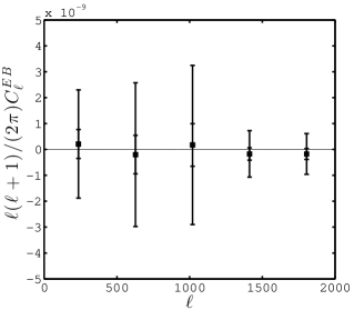
We begin with a verification that the E- and B-mode mass maps are mostly uncorrelated, by comparing their cross-spectra to their respective E- and B- auto-power spectra. We present this measure in Fig. 13, and see that the amplitude is generally lower than $5.0\times 10^{-9}$, whereas both the E and B auto-spectra are more than two orders of magnitude higher, at all multipoles. We therefore conclude that the level of correlation between E and B is consistent with zero. This is not the same as claiming that the $\kappa_{\rm gal}$ maps are free of B-modes, since that contamination would not be detected in that test. It rather shows that if any residual contamination from the B-modes leaked into the E-mode maps, they do not correlate with the true E-modes, hence should disappear in cross-correlations measurements. For measurements and further discussions of B-modes in CFHTLenS and RCSLenS, see Heymans et al. (2012) and Hildebrandt (in prep.).

Figure 13: Cross-spectrum between the E- and B-mode $\kappa_{\rm gal}$ maps measured from the 14 RCSLenS fields with the pseudo-$C_{\ell}$ pipeline P1. The outer error bars represent the $1\sigma$ scatter between the fields, the inner ones are about the mean.

To verify this, we compute the cross-correlation between the Planck lensing maps and the B-mode maps, shown as thick red circles in Fig. 4. The level of B-modes in the cross-correlation is clearly lower than the E-modes for all multipoles. Although this figure shows the results from the P1 pipeline, we verified that this was also the case for P2-P5. Additionally, this B-mode cross-correlation measurement is shown to be consistent with zero in Section 6.1 from a $\chi^{2}$ calculation, which is indicative of a truly successful test. This confirms that if there are true B-modes in the E-mode maps, they do not significantly survive the cross-correlation. We perform this null test on the two configuration-space estimators, shown with red points in Fig. 5, which are also consistent with the null hypothesis.

The next null test consists of rotating the galaxies randomly before performing the map reconstruction and the cross-correlation, which we repeat 100 times. By construction, these randomized $\kappa_{\rm gal}$ realizations are consistent with the noise levels of the $\kappa_{\rm gal}$ maps. Therefore we expect that their cross-correlation with $\kappa_{\rm CMB}$ should be consistent with zero as well. We perform this test on pipeline 1, 2 and 5, and show the results as black points in Fig. 4. These are all in excellent agreement with the null expectations. There is no need to carry this test for P3-4, since zero-padding can not alter the noise levels.

Finally, we perform a cross-correlation of 100 CMB lensing simulations, provided by the Planck 2015 data release, with both the $\kappa_{\rm gal}$ E-modes and B-modes maps, also shown as thin black points in Fig. 4. We see that the mean value is well centred on zero in all pipelines.

From these different tests, we conclude that the level of residual systematics that affect our signal must be much smaller than the statistical error uncertainty. The CFHTLenS and RCSLenS data sets are in excellent condition for cross-correlation science, and no further action needs to taken to recalibrate the measurement.

6 Cosmological Inference

We present in this section our cosmological interpretation of this cross-correlation analysis. We describe the significance of our measurement and compare our results with H15, LH15 and K15. We also discuss the potential contamination by intrinsic alignment, the effect of uncertainty in $n(z)$ and on the $m$-correction, and finally explore the constraining power on various cosmological parameters.

6.1 Significance

Table 3: Summary of $\chi^{2}$ and SNR values obtained with the five different pipelines P. The CFHTLenS dataset has 19 degrees of freedom (5 bins x 4 fields - 1 free parameter), whereas the RCSLenS dataset has 69 (5 bins x 14 fields - 1 free parameter). This is directly reflected in the significantly different $\chi_{\rm min}^{2}$ and $\chi^{2}_{\rm null}$ values between both surveys. The quantities $A^{\rm WMAP9}$ and $A^{\rm Planck}$ are the best-fit amplitudes that scale the theoretical signal, which differ for each pipeline and survey. The values listed here include the covariance debiasing factor $\alpha$ and the extra error $\epsilon$ due to the noise in the covariance (see main text for more details).

	P	$\chi^{2}_{\rm min}$	$\chi^{2}_{\rm null}$	SNR	$A^{\rm WMAP9}$	$A^{\rm Planck}$
CFHTLenS	P1	13.74	18.75	2.24	0.75 $\pm$ 0.34	0.68 $\pm$ 0.31
	P2	12.41	15.80	1.84	0.64 $\pm$ 0.35	0.58 $\pm$ 0.32
	P3	20.01	24.66	2.16	0.77 $\pm$ 0.36	0.70 $\pm$ 0.33
	P4	18.32	21.68	1.84	0.66 $\pm$ 0.37	0.61 $\pm$ 0.33
	P5	14.69	18.64	1.99	0.68 $\pm$ 0.34	0.62 $\pm$ 0.31
RCSLenS	P1	45.27	61.50	4.03	1.44 $\pm$ 0.36	1.31 $\pm$ 0.33
	P2	50.63	67.79	4.14	1.47 $\pm$ 0.36	1.33 $\pm$ 0.33
	P3	42.62	55.55	3.60	1.36 $\pm$ 0.40	1.24 $\pm$ 0.34
	P4	47.43	62.02	3.82	1.54 $\pm$ 0.41	1.39 $\pm$ 0.37
	P5	59.17	66.84	2.77	1.04 $\pm$ 0.39	0.95 $\pm$ 0.34
Combined	P1	57.71	76.00	4.28	1.07 $\pm$ 0.25	0.98 $\pm$ 0.22
	P2	62.23	79.14	4.12	1.04 $\pm$ 0.26	0.95 $\pm$ 0.22
	P3	60.46	75.94	3.94	1.05 $\pm$ 0.26	0.95 $\pm$ 0.25
	P4	64.61	79.26	3.83	1.05 $\pm$ 0.28	0.96 $\pm$ 0.25
	P5	70.34	80.93	3.26	0.84 $\pm$ 0.26	0.77 $\pm$ 0.24

Table 4: Summary of $\chi^{2}$ and SNR values obtained with the two configuration-space statistics. The CFHTLenS and RCSLenS dataset are measured directly on 4 and 6 bins respectively, which explains the different $\chi^{2}$ compared to the Fourier analysis. With one free parameter ($A$), the number of degrees of freedom is $\nu=3$ and $\nu=5$ for the two surveys, when the estimators are analyzed separately. For the joint $\kappa_{\rm CMB}\kappa_{\rm gal}+\kappa_{\rm CMB}\gamma_{t}$ analysis, we have $\nu=7$ and $\nu=11$ respectively. The last row shows the joint estimator analysis for the combined surveys. The error on $A$ includes the covariance debiasing factor $\alpha$ and the extra error $\epsilon$ due to the noise in the covariance.

		$\chi^{2}_{\rm min}$	$\chi^{2}_{\rm null}$	SNR	$A^{\rm WMAP9}$	$A^{\rm Planck}$
CFHTLenS	$\kappa_{\rm gal}$	1.13	5.81	2.16	0.74 $\pm$ 0.36	0.67 $\pm$ 0.33
	$\gamma_{t}$	0.49	5.97	2.34	0.88 $\pm$ 0.41	0.81 $\pm$ 0.37
	both	1.56	7.93	2.53	0.72 $\pm$ 0.30	0.65 $\pm$ 0.28
RCSLenS	$\kappa_{\rm gal}$	2.23	19.06	4.10	1.30 $\pm$ 0.34	1.18 $\pm$ 0.31
	$\gamma_{t}$	4.40	17.70	3.65	1.43 $\pm$ 0.42	1.30 $\pm$ 0.39
	both	9.16	27.84	4.33	1.24 $\pm$ 0.31	1.12 $\pm$ 0.28
Combined	both	12.85	34.17	4.62	1.04 $\pm$ 0.24	0.94 $\pm$ 0.21

The significance of our Fourier-space measurement is quantified by a signal-to-noise ratio (SNR) metric that examines deviations from a pure noise realization, closely following the methods described in LH15, H15 and K15. Under the assumption that the fields are independent, we can ignore their field-to-field covariance and merge the 18 data and prediction vectors; the 18 covariance matrices are then organized into a large block-diagonal matrix. We compute the $\chi^{2}$ statistic as:

$$\chi^{2}={\rm x}\mbox{Cov}^{-1}{\rm x}^{\rm T}$$ (25)

with

$${\rm x}=\hat{C}^{\kappa_{\rm CMB}\kappa_{\rm gal}}-A\widetilde{C}^{\kappa_{\rm CMB}\kappa_{\rm gal}}.$$ (26)

In equation 26, $\hat{C}^{\kappa_{\rm CMB}\kappa_{\rm gal}}$ is the observed pseudo-$C_{\ell}$, $\widetilde{C}^{\kappa_{\rm CMB}\kappa_{\rm gal}}$ is the modelled pseudo-$C_{\ell}$, and a matrix summation is implied. We include a free parameter $A$ that modifies the overall amplitude of the predictions, and can eventually be mapped to combinations of $\sigma_{8}$, $\Omega_{\rm M}$ and other sources of systematic effects. Recall that the predictions are different for each field due to differences in smoothing scales, masks and $n(z)$ distributions. The configuration-space measurements are processed similarly, with the exception that the fields are already merged in each survey, leading to $\chi^{2}$ with fewer degrees of freedom.

The inverse covariance matrix that enters equation 25 is debiased with the correction factor $\alpha=(n-p-2)/(n-1)=0.94$ described in Hartlap et al. (2007), where $p$ is the number of data bins and $n$ is the number of simulations used in the covariance estimation. With $p=5$ and $n=100$, the inverse covariance (or equivalently the $\chi^{2}$) must be lowered by $\alpha^{-1}-1=6\%$. This debiasing scheme is not exact, as noted by Sellentin & Heavens (2016); when sampled from simulations, the inverse of a covariance matrix should be debiased by marginalizing over an inverse-Wishart distribution of the true covariance matrix. Discrepancies between this and the Hartlap et al. (2007) method increase rapidly with lower values of $\alpha$. With $\alpha=0.94$, this would lead to a correction on the $\chi^{2}$ calculated from the inverse covariance in the range $[0-20]\%$, with larger corrections being applied on larger $\chi^{2}$, hence would lower the significance of our measurement by a few percent. We note that H15 and LH15 did not debiased their inverted covariance, while K15 used the Gaussian estimator (equation 23) verified against $N$-body simulations that were debiased with the Hartlap et al. (2007) scheme. We must therefore keep in mind that ignoring the Sellentin & Heavens (2016) correction might slightly affect the significance of our conclusions, as well as that of H15, LH15 and K15.

We then define SNR $=\sqrt{\chi^{2}_{\rm null}-\chi^{2}_{\rm min}}$, where $\chi^{2}_{\rm null}$ is computed by setting $A=0$, and the best-fit value for $A$ is found at $\chi^{2}_{\rm min}$. The error on $A$ is obtained from the one-parameter minimum $\chi^{2}$ method. As discussed in Section 4.3.1, the error on $A$ must be modified by a factor $(1+\epsilon/2)$ as a result of the propagated uncertainty coming from the noise in the covariance matrix (Taylor & Joachimi, 2014). We therefore have $\sigma_{A}\rightarrow\sigma_{A}(1+\epsilon/2)=\sigma_{A}(1+0.07)$, which, for instance, maps $\sigma_{A}=0.3$ to $\sigma_{A}=0.32$. The $\chi^{2}$ and SNR calculations are performed on the coarsely binned measurement, where the inversion of the covariance matrix benefits from data compression. With 5 $\ell$-bins per fields, we expect $\chi^{2}_{\rm min}\sim 19$ for CFHTLenS, $69$ for RCSLenS, and $89$ for the combined set. The results from the Fourier-space analyses are shown in Table 3 for all pipelines, assuming both WMAP9 and Planck cosmologies.

The measured values of $\chi_{\rm min}^{2}$ seem surprising low at first, as one typically expects $\chi^{2}/\nu\sim 1$, where $\nu$ is the numbers of degrees of freedom. Once we factor in the expected uncertainty on the measured $\chi^{2}$ however, this apparent inconsistency is relaxed. Indeed, the error on the $\chi^{2}$ measurement can be calculated as $\sigma_{\chi^{2}}=\sqrt{2\nu}$, which yields $\sigma_{\chi^{2}}=11.7$ and $6.1$ for the Fourier-space analyses of RCSLenS and CFHTLenS respectively. Within $2.2\sigma$, all measured $\chi_{\rm min}^{2}$ from RCSLenS are consistent with $\chi^{2}/\nu\sim 1$, and CFHTLenS are consistent within $1.1\sigma$. This suggests that the error bars on our RCSLenS measurements are slightly overestimated, which implies that our results are conservative. The SNR from RCSLenS roughly doubles compared to that of CFHTLenS, which is solely due to the difference in survey area. Indeed, since the covariance scales as the inverse of the area (neglecting changes in $n(z)$), we can estimate the gain in SNR between the two surveys from $\sqrt{A_{\rm RCS}/A_{\rm CFHT}}=\sqrt{600.7/146.5}=2.02$, which is very close to what we observe.

We find that the CFHTLenS data prefer lower values of $A$, which we loosely interpret as favouring the WMAP9 cosmology, whereas the RCSLenS data prefer higher values, seemingly closer to the Planck predictions. One must be cautious here since many factors are at play that could explain why this is happening even without requiring a change in cosmology, as we discuss in the following sections.

One of the most important result from Table 3 is the observed variations in both SNR and $A$. For the CFHTLenS data, P1 and P3 have the highest values in both of these quantities, and coincide with pipelines in which mask apodization was not applied. This suggests that this procedure has an important impact and should be carefully examined. For RCSLenS, the SNR recovered from the different pipelines vary from 2.77 (P5) to 4.14 (P2), and the values of $A^{\rm Planck}$ vary from 0.95$\pm$0.34 (P5) to 1.39 $\pm$ 0.37 (P4). Pipeline P5 presents the lowest value of $A$, most likely due to the masking of the point sources in the Planck mask. These are regions that carry a significant fraction of the weak lensing signal. Removing them from the analysis suppresses the cross-power at all scales, which translates in a lower $A$, as noted in LH15 and confirmed by our simulations in Section 5.2. A comparison of the $C_{\ell}^{\kappa_{\rm CMB}\kappa_{\rm gal}}$ measurements for P1-P5 (leading to the values entered in Table 3) is presented in Appendix B. It is unfortunate that the expected gain in SNR from pipeline P3 and P4 (with the larger, zero-padded maps) is not directly seen in the Fourier analysis, contrarily to the configuration space. This can be attributed to the fact that zero-padding introduces an additional window function, and that a full forward modelling of this quantity is required in order to recover the gain expected from equation 13. This window function should be incorporated in the mode-mixing matrix formalism, which would then be applied at the end of P3 and P4. Since these two pipelines show no sign of bias, we do not want to introduce inaccuracies in the modelling, hence we decided not to investigate this any further.

We next combine all 18 fields from both surveys to extract a single $A$. We use $n_{\rm CFHT}(z)$ and $n_{\rm RCS}(z)$ accordingly, and follow the steps listed in Section 4.1.1. We update the covariance debiasing term $\alpha$ and the extra sampling variance term $\epsilon$ for a measurement made with 10 data points. The results are shown in the lower section of Table 3 (labelled ‘Combined’), where we see an overall increase in significance, up to SNR = 4.28 for the pseudo-$C_{\ell}$ pipeline P1. We also recover a best fit value for $A$ that is in excellent alignement with both the WMAP9 and Planck predictions, however we are not able to distinguish between the two.

We repeat this measurement with the configuration-space estimators and present the results in Table 4 for $\xi^{\kappa_{\rm CMB}\kappa_{\rm gal}}$, $\xi^{\kappa_{\rm CMB}\gamma_{t}}$ and for the combination of both data vectors. With 6 bins per estimator in the RCSLenS measurements, the covariance de-biasing factors becomes a 3.5% correction on the SNR, and 6.5% for the joint $\xi^{\kappa_{\rm CMB}\kappa_{\rm gal}}+\xi^{\kappa_{\rm CMB}\gamma_{t}}$ analysis. We recover the same trends as the Fourier analysis: CFHTLenS prefers the lower values of $A$, RCSLenS prefers higher values, and the actual values of $A$ agree within $1\sigma$ with the Fourier analyses. We also note that $\gamma_{t}$ prefers higher $A$, as already seen in Fig. 5. This has a very low significance given the size of the error bars, and is likely due to the different physical scales probed by the estimators. By construction, for a fixed $\vartheta$ the estimator $\kappa_{\rm CMB}\kappa_{\rm gal}$ is more sensitive to larger angular scales compared to $\kappa_{\rm CMB}\gamma_{t}$, largely because of the $J_{2}$ term that appears in equation 8. Consequently, in order to correctly probe the $\kappa_{\rm CMB}\gamma_{t}$, the measurement needs to reach larger angles. We verified in Section 5.3 that both $\kappa_{\rm CMB}\kappa_{\rm gal}$ and $\kappa_{\rm CMB}\gamma_{t}$ give consistent results on simulations, hence the difference cannot be attributed to a mis-calibration of the estimators. Because all points are highly correlated and the preference is only a $1\sigma$ effect, we do not investigate this any further. As for the Fourier-space analyses, the $\chi^{2}$ values are lower than expected. However, the same consistency applies to the configuration-space measurements, In which the measured values are found to be within $2\sigma$ of the expected values. Here, $\nu=5$ and 3 for the RCSLenS and CFHTLenS surveys, from which we get $\sigma_{\chi^{2}}=3.2$ and $2.4$. For the combined $\xi^{\kappa_{\rm CMB}\kappa_{\rm gal}}+\xi^{\kappa_{\rm CMB}\gamma_{t}}$ statistics, $\nu$ = (12-1) and (8-1) respectively.

As mentioned earlier, the SNR measured in the RCSLenS and CFHTLenS with all three estimators are similar and consistent within $\sim 1\sigma$. Additionally, we find a mild gain in combining both $\xi^{\kappa_{\rm CMB}\kappa_{\rm gal}}$ and $\xi^{\kappa_{\rm CMB}\gamma_{t}}$, due to the slightly different dynamical regions that are probed. We see this reflected in the SNR values, which show increases of about 6%, achieving the highest significance of our paper this way, with SNR=4.62 for CFHTLenS and RCSLenS combined. Due to the limited number of CMB lensing simulations however, we do not explore the combination with Fourier analysis, but this should certainly be considered in the analysis of upcoming survey.

It may seem surprising that the error on $A$ seems almost unchanged between CFHTLenS and RCSLenS, since the error about the cross-correlation measurement is more precise by a factor of 2. What needs to be taken into account in the survey comparison is that the value of $A$ are quite different, hence it is the fractional error about $A$ that needs to be examined. From both Tables 3 and 4, we can see that the quantity $\sigma_{A}/A$ has dropped by almost a factor of two, which is how the improvement should be assessed (this scaling is naturally reflected in the SNR metric).

As an additional verification, we asserted from a $\chi^{2}$ calculation that the B-mode measurements are all consistent with zero. Given a WMAP9 cosmology, the preferred amplitude is $\left|A\right|<0.15$ in all pipelines, with a detection significance of SNR $\lesssim$ 0.7. In comparison, the preferred amplitude for E-modes is closer to unity, with a significance of SNR $\sim$2-4 depending on the survey. This quantitative test gives us additional confidence that our measurement is not affected by B-mode contamination.

6.2 Propagation of uncertainty about $n(z)$

As discussed in H15, the cross-correlation signal is significantly affected by the uncertainty on the source distribution. For instance, if some sources with higher true redshift leak into the low-redshift part of the $n(z)$ due to a wrong photometric estimation, it will cause a significant mis-match between the predictions and measurement. The converse is equally true, and most of the challenge resides in modelling accurately the high-redshift tail of the distribution. This tail is the least accurate regime of the photo-$z$ measurements, but at the same time it is the section of the $n(z)$ that maximally contributes to the signal – mostly due to the shape of the geometric kernel $W^{\rm CMB}$.

Choi et al. (2015) found evidence from spec-$z$/photo-$z$ cross-correlations that the stacked PDF calculated from the BPZ software was not quite accurate, such that both the CFHTLenS and RCSLenS $n(z)$ were biased. The redshift of the peak in $n_{\rm RCS}$ is at worst contained within $\Delta z=^{+0.24}_{-0.1}$ of the value found from the weighted stacked PDF. This was obtained in the context of tomographic analyses where the full redshift distribution is split in a number of narrow redshift bins, while most of this bias cancels in broader bands (Hildebrandt, in prep.). Consequently, we do not apply any peak shift in the data, but instead examine how our uncertainty on the $n(z)$ affect the predictions, as described below. It was shown in H15 that while holding the cosmological parameters fixed, variations on the peak of the $n(z)$ and on the high-redshift tail could lead to changes of order $10\%-20\%$ in the amplitude of the predictions, a precision level that likely also applies to CFHTLenS. However, the fact that H15 used a COSMOS-matched sample to extend their redshift distribution to higher $z$ probably introduced additional calibration errors. For our CFHTLenS selection criteria, a 10% precision is more likely. The RCSLenS survey is shallower, hence variations in $n(z)$ coupled with a steeper slope in $W^{\rm CMB}$ could decrease the precision even more.

In comparison to the the analysis of Choi et al. (2015), the redshift of our RCSLenS sample is known to a higher accuracy, thanks to the GALEX UV measurement. When compared to the VIPERS spectroscopic data, Moutard et al. (2016) found a systematic bias in the mean photo-$z$ estimation of the CFHTLenS+GALEX data. Although negligible for $z_{phot}<1$, the difference $z_{phot}-z_{spec}$ increases linearly and reaches 50% by $z_{phot}=1.8$. This bias is caused by mis-identified high-redshift outliers that have a matched $z_{spec}$ much closer to 0.5. The rate of outlier $\eta_{\rm out}$ is consistent to zero up to $z_{phot}=1.0$, then is well modelled as

$$\eta_{\rm out}(z_{phot})=0.75(z_{phot}-1).$$ (27)

These VIPERS-CFHTLenS galaxies are broadly distributed in the $i$-band magnitudes range 22-24. RCSLenS $r$-band data has a similar depth, and it reasonable to assume that the same level of outlier rate applies to the RCSLenS galaxies. We next split $n(z)$ into two terms: 1) the ‘correct’ photo-$z$ term that contributes a fraction $(1-\eta_{\rm out}(z))n(z)$ to the full redshift distribution, and 2) the ‘outliers’ term, that contributes a fraction $\eta_{\rm out}(z)n(z)$. The population of outliers peaks between $z=1.0$ and $2.0$, and we redistribute it with the transform: $\eta_{\rm out}(z)n(z)\rightarrow\eta_{\rm out}(z/3)n(z/3)$. This maps the second term on to a smooth peak centred on $z=0.5$, closely matching the observed $z_{spec}$ distribution of the outliers. We finally add this modified second term to the first and insert this new $n(z)$ in our predictions. This procedure is illustrated in the bottom panel of Fig. 14: the two bell-shape curves show the distribution of outliers before (right) and after (left) this mapping, which transforms the black solid $n(z)$ to the black dashed $n(z)$. This modification is then propagated into the prediction in the top and middle panels, from which we can see that this represents a $15\%$ systematic uncertainty on the amplitude of the signal, caused by the outliers. We also see that the scale dependence of this systematic bias can be safely neglected.

Another source of uncertainty in the $n(z)$ comes from the choice of functional form, which is mostly weighted by the low- and medium-redshift section of the distribution, then extrapolated to high redshifts with some arbitrary power law. By construction, the fit will never convincingly match the sparse data, even though the galaxies at high redshift are those that contribute the most to the cross-correlation signal. It then becomes debatable whether one should use functions or the actual $n(z)$ histogram when calculating the predictions. Since our RCSLenS $n(z)$ derives from CFHTLenS+VIPERS photometry, it is also probable that some features seen in the high redshift end of the distribution do not exist in the data, causing yet another bias in the results. In light of this, we examine the consequence of modifying the high-redshift tail on the predictions. We do so by rejecting the high-redshift part of the $n(z)$ with three cuts, at $z=1.8$, $z=2$ and $z=3$, rescaling at each time to preserve the area under the curve. When these cuts are applied, we find from Fig. 14 that the amplitude of the signal drops by $<3.5\%$ in the worst case, with very little angular dependence for $\ell>200$. This means that it can be captured as a small multiplicative factor in front of the theoretical prediction, and is subdominant compared to the photometric redshift outliers.

Figure 14: (top:) Cross-spectrum predictions for a series of modifications applied to $n(z)$: the effect of excluding the high-redshift tail with different cuts (magenta, blue and red dashed), and the reassignment of the catastrophic outliers (black dashed). (middle:) Fractional difference of the cross-correlation signal with respect to the fiducial RCSLenS $n(z)$, for each curve shown in the top panel. (bottom:) Source redshift distribution for two of these modifications. The vertical line shows the redshift cut at $z=1.8$ that produces the red dashed curve. The two dashed blue bell-shape curves represent the distribution of outliers before (right) and after (left) the correction that produces the black dashed curve. Their amplitudes are multiplied by a factor of 15 in this plot.

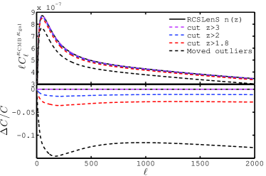
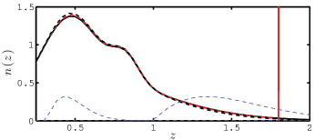
It was suggested recently by Liu et al. (2016) that an incorrect calibration of the shear signal data could possibly result in large systematic effects in the cross-correlation measurement. Indeed, the multiplicative correction $m$-term can be subject to residual systematics effect that could directly leak into the signal as $A\propto(1+m)$. If a wrong $m$ was leading the systematic budget in our measurement, a corrected $m$ would have to be allowed to take values as high as $m=0.73$ and as low as $m=-0.27$ to ensure $A=1$ in all pipelines and for both cosmologies. Liu et al. (2016) and Baxter et al. (2016) remove priors on $m$ and allow even more extreme values. However these $m$ values would be in addition to the $m$ calibration that we have already applied to our analysis based on the image simulations presented in Miller et al. (2013). Whilst these have their limitations (see Kuijken et al., 2015, for a discussion), it is unlikely that the measured $m$ calibration could be so biased. In contrast, biases on photometric redshifts described in this section are of greater importance. Therefore, we do not allow for residual biases on $m$ not captured by the image simulation in Miller et al. (2013), as these are expected to be at the level of less than $\sim$5% (Kuijken et al., 2015), resulting in $\sim$5% errors on $A$. We apply the $m$-correction recommended by the CFHTLenS and RCSLenS teams, and any residual biases would have to be propagated on $A$.

To conclude this section, the impact of all $n(z)$-induced systematic effects are included as a 15% uncertainty on the cosmological information extracted from the amplitude term $A$ defined in equation 25; no uncertainty on the $m$-correction is explicitly included.

6.3 Contamination by intrinsic alignment

In addition to the $\kappa_{\rm CMB}\kappa_{\rm gal}$ signal, CMB lensing correlates with the intrinsic alignment (IA) of foreground galaxies. Galaxies located in the same cluster are connected by tidal forces, which also play a role in determining their intrinsic orientation (for a recent review, see Kirk et al., 2015a). This $\kappa_{\rm CMB}$-IA correlation therefore contributes as an additive secondary signal whose shape and amplitude depend on $n(z)$. as shown in Hall & Taylor (2014) and Troxel & Ishak (2014). Unfortunately, there is a large uncertainty in the modelling aspects of IA, as summarized in Kiessling et al. (2015).

For source redshift distributions similar to CS82, Hall & Taylor (2014) found that this effect could account for 15-20% of the $\kappa_{\rm CMB}\kappa_{\rm gal}$ measurement, which would be higher in absence of IA. Further investigation by Chisari et al. (2015) revealed that the strength of the contamination also depends on the galaxy type. For $n(z)$ similar to that of CS82, they found that IA from red galaxies alone could contribute to $\sim$10% of the signal; the blue galaxies are still consistent with no alignment, but given the current uncertainty, it could also double the total $\kappa_{\rm CMB}$-IA.

In both of these studies, the contamination decreases (increases) for deeper (shallower) surveys: Chisari et al. (2015) estimated that lowering the peak of $n(z)$ by $\Delta z=0.1$ increases the contamination by 15%. Another 20% increase can also be encountered if the high-redshift tail is given more weight. We show the $n(z)$ from CS82, CFHTLenS and RCSLenS in Fig. 1, and find that the peak of the CFHTLenS source distribution is lower than that of CS82 by about $\Delta z=0.1$, but that its high-redshift tail is also lower. These two differences act in opposite directions, such that $\kappa_{\rm CMB}$-IA in both surveys should be similar. In comparison, the RCSLenS is much shallower and its source distribution peaks at $z=0.5$. Surprisingly, we find that it is in fact very similar to the CS82 $n(z)$ once shifted by $\Delta z=0.2$ (labelled ‘CS82 shifted’ in Fig. 1), especially at the high-redshift end. From the peak-shift dependence described in Chisari et al. (2015) and assuming the non-linear model of intrinsic alignement (Bridle & King, 2007), we can estimate that the $\kappa_{\rm CMB}$-IA contamination from the red galaxies in RCSLenS should contribute to about 13% of the signal.

According to Hall & Taylor (2014) and Chisari et al. (2015), the overall scale dependence of $\kappa_{\rm CMB}\mbox{-IA}/(\kappa_{\rm CMB}\kappa_{\rm gal}+\kappa_{\rm CMB}\mbox{-IA})$ is relatively flat, with at most $\sim 50\%$ deviations about its mean in the linear IA model, and possibly as low as $\sim 20\%$ in the non-linear IA model. Given the current uncertainty in our measurement, we are not sensitive to deviations from flatness, hence we can safely treat IA as a multiplicative contribution to our signal. In other words, we effectively treat the amplitude parameter $A$ from equation 25 as a sum of two terms: $A=A_{\rm th}+A_{\rm IA}$. From the above discussion, we can estimate the $A_{\rm IA}$ terms to be $0.13$ and $0.09$ for RCSLenS and CFHTLenS respectively. In the SNR calculation, we do not correct the data nor the predictions for the IA part, which means that either the data are biased low, or the models are biased high. If we opted for the former option, we would increase the SNR of the measurement, but this seems artificial at this point.

We must also mention that Larsen & Challinor (2015) found that within the tidal torque alignement model, the $\kappa_{\rm CMB}$-IA contamination acts in the opposite way, namely the contamination tends to increase the signal, which would be lower without IA. This clearly illustrates the need for development in the field of IA before one can draw more precise conclusions from our cosmological measurement. In the meantime, any interpretation that rely on the merged $A_{\rm th}$ and $A_{\rm IA}$ quantities should be robust against this uncertainty.

6.4 Comparison with previous results

H15 reported the first detection of the galaxy lensing CMB lensing cross-correlation by combining the data from the ACT and the CS82 surveys. Due to the high resolution of the ACT lensing maps, it was possible to extract the signal with a significance of $4.2\sigma$, over a contiguous unmasked area of 121 deg. sq. This area is comparable in size to the sum of the 4 CFHTLenS fields. The redshift distribution from CS82 peaks at $z\sim 0.7$ with mean at $0.9$, and is obtained from a COSMOS (Scoville et al., 2007) matched sample, leading to important uncertainty in the exact $n(z)$ due to sampling variance. Marginalizing over this, they found $A^{\rm Planck}=0.78\pm 0.18$ and $A^{\rm WMAP9}=0.92\pm 0.22$, which translates into a $\sim 12\%$ constraint on $\sigma_{8}(z=0.9)$. They identified the uncertainty in $n(z)$ and the unknown level of contamination by intrinsic alignment (see Section 6.3) as their dominant limiting factor.

The analysis performed by LH15 examined the cross-correlation between all four CFHTLenS fields and the Planck full sky lensing maps. The galaxy selection function differs from the one used in this paper, as they included $z_{B}>1.3$ galaxies, with $n(z)$ modelled from COSMOS. This choice was motivated by an increase in SNR, even though it introduced an uncertainty on $n(z)$ in the range 10-20%. They found evidence for the signal with a significance SNR=$1.9\sigma$ and $2.0$, for the 2013 and 2015 Planck releases respectively. The difference in significance with H15 can be largely attributed to the higher noise level present in the Planck lensing maps, compared to ACT. Following an analysis similar to H15, they found $A^{\rm Planck}=0.44\pm 0.22$ and $A^{\rm WMAP9}=0.52\pm 0.26$, from the Planck 2015 data. The low values of $A$ were unexpected and attributed to uncertainty in $n(z)$ distribution $(\simeq 10\%)$, masking of point sources in the CMB lensing analysis $(\simeq 15\%)$ and intrinsic alignment $(<10\%)$. Nevertheless, from a simple parameterization of the cosmology dependence of the signal, they were able to measure $\sigma_{8}(\Omega_{\rm M}/0.27)^{0.41}=0.63^{+0.14}_{-0.19}$.

From our measurement of the Planck 2015 lensing - CFHTLenS cross-correlation, we are able to recover their results with our method P5 - which is the closest match to that of LH15 - and obtain $A^{\rm WMAP9}=0.63\pm 0.31$, and $A^{\rm Planck}=0.58\pm 0.28$. As seen from Table 3, pipeline P5 favours values of $A$ that are lower by as much as 15%, compared to P1, which has the highest SNR. This is exactly the level of bias that was claimed by LH15 to be caused by cluster masking in the Planck map. Recall that P5 is the only one for which the Planck mask is applied on the $\kappa_{\rm gal}$ maps, thereby rejecting the important contribution from many clusters in the cross-correlation. This bias is even more pronounced in the RCSLenS measurement. A more detailed analysis of this bias could be further investigated from hydrodynamical simulations or within the halo model, but such a study falls outside the scope of this paper. Results from our $N$-body simulations detailed in Section 5.1 suggest that masking the densest regions could reduce the signal by as much as a factor of 2, which would explain and release the tension with the Planck cosmology observed in LH15. The fact that we do not multiply the masks in P1-4 makes a large difference, since the clusters that are masked in the $\kappa_{\rm CMB}$ are un-masked in $\kappa_{\rm gal}$ and can therefore contribute to the signal, at least partially. Indeed, Fig. 5 shows that there is a significant signal even beyond a degree, thereby exceeding the angular size of the largest masked point sources in the Planck CMB lensing maps. Aside from this, all our CFHTLenS measurements agree with both Planck and WMAP9 predictions to within $1.5\sigma$. We obtain similar results from our configuration-space estimator $\kappa_{\rm CMB}\kappa_{\rm gal}$, with $A^{\rm WMAP9}=0.61\pm 0.32$, and $A^{\rm Planck}=0.55\pm 0.29$.

From the measurements of DES $\times$ Planck and SPT lensing, K15 reported $A^{\rm Planck}_{\rm Planck}=0.86\pm 0.39$ and $A^{\rm Planck}_{\rm SPT}=0.88\pm 0.30$, respectively. As opposed to LH15, they find no evidence of tension with the Planck cosmology. In their analysis, the bright clusters were also masked from the SPT lensing map, however these regions were filled from a Wiener filter interpolation, such that the mask has no small scales structures in it. The cross-correlation measurement was carried out with the PolSpice software (Szapudi et al., 2001), which deals properly with distinct masks without multiplying them. This strategy is therefore similar to our method P1.

A clear feature seen in both Tables 3 and 4 is that RCSLenS favours higher values of $A^{\rm Planck}$ compared to Planck $\times$ CFHTLenS, SPT$\times$ DES and Planck $\times$ DES, generally higher than unity. This is not too surprising since all these measurements are extracted from different parts of the sky, and fluctuations are expected. All our measurements are consistent with $A=1$ within $1.3\sigma$.

6.5 Sensitivity to baryons and massive neutrinos

Figure 15: Effect of baryon feedback and massive neutrinos on the cross-correlation signal, compared to a $\Lambda$CDM model (WMAP9) with massless neutrinos and no feedback (‘DM-ONLY’ model). The dotted magenta line shows the ‘AGN’ model extracted from the OWL simulations (van Daalen et al., 2011), while the dashed blue lines represent, from top to bottom, the effect of massive neutrinos with $\Sigma m_{\nu}$ = 0.2 and 0.6eV. The 0.4eV models fall in the middle hence are not shown. Solid red lines show the combined effect. The RCSLenS measurement shown here has been processed with pipeline P2, and models are scaled by the best fit amplitude $A$ = 1.47 (see Table 3). The error bars shown are estimated from the full covariance matrix.

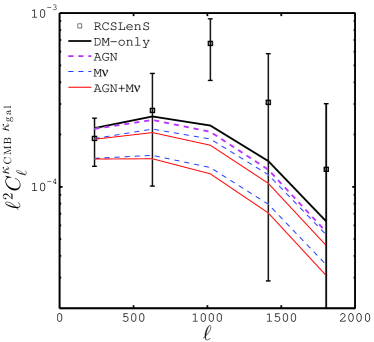
The CMB lensing $\times$ galaxy lensing measurements discussed in this paper can serve as an additional probe, providing an extra constraint on the parameters that describe intrinsic alignment, redshift distributions and cosmology. While H15 and LH15 have already set constraints on $\Omega_{\rm m}$ and $\sigma_{8}$, we examine here the possibility to jointly weigh the neutrinos and constrain galaxy evolution models through their feedback on the total matter density.

For our predictions, we following the strategy of Harnois-Déraps et al. (2015), which includes the joint neutrino+baryon effects with two independent multiplicative terms. First, baryonic effects on the cross-correlation functions are implemented via their impact on the matter power spectrum, $P(k,z)$, as measured in van Daalen et al. (2011). These are based on the OverWhelmingly Large (OWL) simulations (Schaye et al., 2010), an ensemble of cosmological hydrodynamical simulations that include realistic astrophysical processes and feedback mechanisms coming from supernovae, AGN, stellar winds, etc. (Schaye et al., 2010). Among the available models we selected the one named ‘AGN’. According to van Daalen et al. (2011), this model provides the best fit for a number of observations. We compute the relative effects compared to the OWL ‘DM’ model, a dark matter only universe, and define the baryon feedback bias as:

$$b^{2}_{\rm AGN}(k,z)\equiv\frac{P^{\rm AGN}_{\rm OWL}(k,z)}{P^{\rm DM}_{\rm OWL}(k,z)},$$ (28)

Second, we include massive neutrinos with total mass $M_{\nu}=\sum m_{\nu}$ = 0.2, 0.4 and 0.6eV in a similar manner, using their implementation in the CAMB numerical code (Lewis et al., 2000) to compute the massive neutrino bias relative to the $\sum m_{\nu}=0.0$eV case:

$$b^{2}_{M_{\nu}}(k,z)\equiv\frac{P^{{\rm DM}+M_{\nu}}_{\rm CAMB}(k,z)}{P^{\rm DM}_{\rm CAMB}(k,z)},$$ (29)

We model the impact of massive neutrinos and baryon feedback on our fiducial model from these two biases:

$$P^{{\rm AGN}+M_{\nu}}(k,z)=P^{\rm fid}(k,z)\times b^{2}_{M_{\nu}}(k,z)\times b^{2}_{\rm AGN}(k,z).$$ (30)

This assumes that both effects can be treated separately, which is known to hold at least up to $k=8h{\mbox{Mpc}}$ (Bird et al., 2012). The same conclusion are reached from a halo model approach in Mead et al. (2016). By feeding the results from equation 30 into equation 5, we propagate these two effects onto $C_{\ell}^{\kappa_{\rm CMB}\kappa_{\rm gal}}$.

Fig. 15 shows the impact of massive neutrinos and baryonic feedback on the cross-spectrum, relative to a $\Lambda$CDM universe. We see that the presence of massive neutrinos (dashed blue) affects all scales, causing a suppression that varies from 10% to 50% in the mass range that we probe, and is maximal at $\ell\sim 2000$. This effect is partly degenerate with a decrease in $\Omega_{\rm M}$ and $\sigma_{8}$, as well as with the contamination by intrinsic alignment and incorrect estimation of the $n(z)$, although these do not have the exact same scale dependence.

Similar conclusions can be drawn for the prospect of constraining baryonic feedback models with this measurement. The distinctive features of the AGN model are mostly felt at $\ell>1000$, which has a characteristic tilt that might be easier to capture than the neutrino mass. In the optimistic scenario where $\Omega_{\rm M}$ and $\sigma_{8}$ are fixed by the large scale measurements or other cosmological probes, the shape of the cross-correlation with respect to a $\Lambda$CDM universe can serve to constrain baryonic and neutrino physics. For these two effects to be measured however, the analysis needs to include very small angular scales that are usually excluded when considering baryon feedback as nuisance.

Also plotted in Fig. 15 is the RCSLenS data using pipeline P2, which shows the highest SNR. Given the current level of uncertainty, it is not possible to place constraints on any of these effects, but it becomes clear that they cannot be neglected in upcoming surveys without biasing low the best-fit values of $\sigma_{8}$ and $\Omega_{\rm M}$. In order to reject some of the models shown here, the size of the error bars will need to shrink by at least a factor of 3, calling for survey combinations whose common area is of the order of a few thousands square degrees such as DES or KiDS, or with CMB lensing maps with less noise such as ACT and SPT. High hopes are placed on upcoming surveys to improve this measurement.

Note finally that the $\ell$-dependence of the IA contamination can cause some confusion in the search for the scale-dependent features in the signal left by baryonic feedback and massive neutrinos. However, their signatures are likely to be stronger than that of IA, causing suppression of up to 50% (see Fig. 15), versus $\sim 10$% for IA, and therefore still measurable.

7 Conclusion

Cross-correlation measurements between two independent cosmological datasets are potentially free from contamination by residual systematics. As such they can be treated as distinct and possibly cleaner probes of the large scale structure. In this paper, we combine the public Planck 2015 lensing map with the CFHTLenS and RCSLenS data and extract the cross-correlation signal with a significance of $\sigma=4.62$. The combined galaxy surveys cover a total unmasked area of 747.2 deg², a factor of four larger than previous measurements by H15, LH15 and K15. Whereas these three papers focused on the Fourier-space estimator $C_{\ell}^{\kappa_{\rm CMB}\kappa_{\rm gal}}$, we present here the first configuration-space measurements. We achieve this with two different estimators, $\xi^{\kappa_{\rm CMB}\kappa_{\rm gal}}$ and $\xi^{\kappa_{\rm CMB}\gamma_{t}}$, and find an excellent agreement between the configuration-space and Fourier-space approaches, providing extra confidence in the accuracy of our results. Since the estimators probe slightly different scales, they are in that sense complementary, and we achieve a small gain in SNR by combining them. More importantly, the main advantage of these configuration-space estimators is that they are less affected by mask-induced effects.

The three previous $C_{\ell}^{\kappa_{\rm CMB}\kappa_{\rm gal}}$ measurements used different methods and datasets, and it is unclear which technique is optimal. Moreover, tracking potential systematic effects across them becomes highly challenging. To address this important issue, we repeated our analysis using five different pseudo-$C_{\ell}$ pipelines and investigated their impact on both the SNR and the cosmological results. We find important differences, largely due to changes in the implementation of the masks, but these are not distinguishable in the data given the current statistical precision. These pipelines are verified against a suite of high resolution $N$-body simulations, and favour strategies in which the CMB and galaxy masks are not combined and applied to the two datasets, as opposed to the approach used in previous studies. Mask multiplication reduces the SNR and biases low the amplitude of the measured signal.

We finally compare our measurements against theoretical models that include massive neutrinos and baryonic feedback, and show that these can easily be confused with intrinsic alignment contamination or offsets in the source redshift distribution. For instance, neutrinos with mass $M_{\nu}-0.2$eV produce a suppression of about 10-15% at all scales, just as the preferred IA models. We also estimate that our signal could be biased similarly by the photometric redshift outliers. Some baryonic feedback models like the OWL-AGN predict a significant suppression with a tilt that is more pronounced and harder to reproduce by other secondary signals. There is thus hope that future experiments will offer significant constraining power on neutrinos and baryon physics, once we overcome the challenges related to the modelling of IA contamination and to the photometric redshift measurements.

Appendix A Forward modelling

Figure 16: Cross-spectra between the RCSLenS masks and the Planck 2015 masks, over-plotted for each of the 14 RCSLenS fields. Top to bottom panels are for pipelines 1 to 5. All measurements are normalized such that their lowest $\ell$-mode coincide, in order to show the level of mode-mixing that enters equation 39. The suppression of mode-mixing due to apodization is clearly visible here. The two fields which show the largest amount of cross-correlation for $\ell>200$ (causing larger mode-mixing) are CDE0310 and CSP0320.

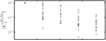
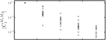
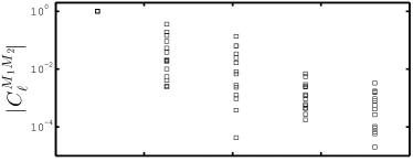
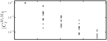
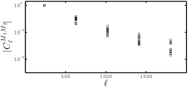
This section describes our forward modelling algorithm, which turns a theoretical $C_{\ell}^{\kappa_{\rm CMB}\kappa_{\rm gal}}$ into a pseudo-$C_{\ell}$ that can then be compared against the Fourier-space measurements detailed in Section 4.1.5. At the core of this procedure is the calculation of the mode-mixing matrix, which is sensitive to the analysis masks $M_{i}$. Since these masks vary for different fields ‘$i$’, the pseudo-$C_{\ell}$ are field-dependent quantities and are therefore written as $\widetilde{C}_{\ell}^{\kappa_{\rm CMB}\kappa_{\rm gal},i}$. The derivations presented here are adapted from the cosmic shear method described in Asgari et al. (in prep.) in the context of $\kappa_{\rm CMB}$-$\kappa_{\rm gal}$ cross-correlations.

The very first step consists in interpolating the $C_{\ell}^{\kappa_{\rm CMB}\kappa_{\rm gal}}$ predictions (from equation 5) in fine $\ell$-bins (these are unique for each field, see Section 4.1.5). This ensures that the binning process does not create biases between the data and theory. We next combine these predictions with the field masks. For the sake of clarity, let us assume first that the underlying $\kappa$ maps are unbiased, such that $\widetilde{C}_{\ell}^{\kappa_{\rm CMB}\kappa_{\rm gal},i}$ can be expressed as a convolution between the underlying $C_{\ell}^{\kappa_{\rm CMB}\kappa_{\rm gal}}$ and the Fourier transform of the mask, $W^{i}(\ell)$. When measuring the auto-spectrum, $C_{\ell}^{\kappa}$, this procedure can be written as (Hivon et al., 2002):

$$\widetilde{C}_{\ell}^{\kappa,i} = \left\langle\int\!\!C_{\ell^{\prime}}^{\kappa}\left|W^{i}({\boldsymbol{\ell}}-{\boldsymbol{\ell}}^{\prime})\right|^{2}\mbox{d}^{2}{\boldsymbol{\ell}^{\prime}}\right\rangle_{\Omega},$$ (31)

where the angle brackets refer to the angular averaging of $\boldsymbol{\ell}$, i.e. $\langle...\rangle_{\Omega}=(2\pi)^{-1}\int...\mbox{d}\Omega$, and $\mbox{d}^{2}{\boldsymbol{\ell}^{\prime}}=\ell\mbox{d}\ell\mbox{d}\Omega$. We can generalize the above results to the cross-spectrum between any maps $\kappa_{1}$ and $\kappa_{2}$ as

$$\widetilde{C}_{\ell}^{\kappa_{1}\kappa_{2},i} \equiv \left\langle\int\!\!C_{\ell^{\prime}}^{\kappa_{1}\kappa_{2}}\left[W_{1}^{i}(\boldsymbol{L})W_{2}^{i*}(\boldsymbol{L})\right]\mbox{d}^{2}{\boldsymbol{\ell}^{\prime}}\right\rangle_{\Omega},$$ (32)

where we defined ${\boldsymbol{L}}={\boldsymbol{\ell}}-{\boldsymbol{\ell}}^{\prime}$. Note that in the above two expressions, there are two angular integrations, running over $\Omega$ and $\Omega^{\prime}$, the polar angles of the vectors $\boldsymbol{\ell}$ and $\boldsymbol{\ell}^{\prime}$ respectively. Assuming that the true convergence cross-spectrum $C_{\ell}^{\kappa_{1}\kappa_{2}}$ is isotropic, it can be taken outside of the two angular integrations:

$$\widetilde{C}_{\ell}^{\kappa_{1}\kappa_{2},i} = \!\!\int\!\!C_{\ell^{\prime}}^{\kappa_{1}\kappa_{2}}\left[\left\langle W_{1}^{i}(\boldsymbol{L})W^{i*}_{2}(\boldsymbol{L})\right\rangle_{\Omega,\Omega^{\prime}}\right]\ell^{\prime}\mbox{d}\ell^{\prime}.$$ (33)

Let us focus on the inner bracketed term, which is averaged over both $\Omega$ and $\Omega^{\prime}$. Under the change of variables $\Omega_{L}\equiv\Omega+\Omega^{\prime}$ and $\eta\equiv\Omega-\Omega^{\prime}$, we can write d$\Omega$d$\Omega^{\prime}$ = 2d$\Omega_{L}$d$\eta$, where $\Omega_{L}$ can be identified as the polar angle of $\boldsymbol{L}$. In this $\{\Omega_{L},\eta\}$ coordinate system, the double integration over the mask cross-spectra simplifies greatly:

$$\left\langle W_{1}^{i}(\boldsymbol{L})W^{i*}_{2}(\boldsymbol{L})\right\rangle_{\Omega,\Omega^{\prime}} = \int\!\!\!\!\int\!\!W_{1}^{i}(\boldsymbol{L})W^{i*}_{2}(\boldsymbol{L})\mbox{d}\Omega\mbox{d}\Omega^{\prime}$$ (34)

$$= 2\!\!\int_{0}^{\pi}\!\!\mbox{d}\eta\!\!\int\!\!W_{1}^{i}(\boldsymbol{L})W^{i*}_{2}(\boldsymbol{L})\mbox{d}\Omega_{L}$$ (35)

$$= 4\pi\!\!\int_{0}^{\pi}\!\!W_{1}^{i}(L)W^{i*}_{2}(L)\mbox{d}\eta.$$ (36)

Written in this form, the angular dependence of $L$ vanishes; the integrand is simply the angle-averaged cross-spectrum of the two masks, $C_{\ell}^{M_{1}M_{2}}$, which is easy to compute as a separate step, for each of the 5 pipelines under investigation in this paper. The mask cross-spectra are provided in Fig. 16, for methods P1-5. These are measured separately for each of the 14 RCSLenS fields, rebinned in the final coarse binning scheme, and over-plotted in this figure. Only three fields out of the 18 have cross-spectrum elements that are higher than 10%, which indicates that the effects of mode-mixing, averaged over the 18 fields, should be minor. The integral in equation 36 runs over $\eta$, which can be identified – from the change of variable described below equation 33 – as the angle between $\boldsymbol{\ell}$ and $\boldsymbol{\ell}^{\prime}$. From the law of cosines, we can write $L^{2}=\ell^{2}+\ell^{\prime 2}-2\ell\ell^{\prime}\mbox{cos}\eta$, which maps $\eta$ to $L$ given a pair $\{\ell,\ell^{\prime}\}$, and finally perform the integral numerically. The term on the left hand side of equation 36 is the mode-mixing functional $\mathcal{M}^{i}(\ell,\ell^{\prime})$ and applies in the continuous case. We can rewrite equation 33 as:

$$\widetilde{C}_{\ell}^{\kappa_{1}\kappa_{2},i} \equiv \!\!\int\!\!C_{\ell^{\prime}}^{\kappa_{1}\kappa_{2}}\mathcal{M}^{i}(\ell,\ell^{\prime})\ell^{\prime}\mbox{d}\ell^{\prime}.$$ (37)

Turning the integral into a discrete sum, and absorbing all normalization factors in this process, we finally obtain the mode-mixing matrix ${\rm M}_{\ell\ell^{\prime}}^{i}$ as:

$$\widetilde{C}_{\ell}^{\kappa_{1}\kappa_{2},i} = \sum_{\ell^{\prime}}C_{\ell^{\prime}}^{\kappa_{1}\kappa_{2}}\mathcal{M}_{\ell\ell^{\prime}}^{i}\ell^{\prime}\Delta\ell^{\prime}$$ (38)

$$\equiv {\rm M}_{{\ell}{\ell^{\prime}}}^{i}C_{\ell^{\prime}}^{\kappa_{1}\kappa_{2}}.$$ (39)

The smoothing of the maps can be included at this stage by multiplying the results by the appropriate kernels $\left|S_{1}^{i}(\ell)S_{2}^{i}(\ell)\right|$, which are typically Gaussian functions. To simplify the notation further, this term can be absorbed in the definition of $\rm M_{\ell\ell^{\prime}}^{i}$. We could then use equation 39 to propagate the effect of masking and smoothing on the theoretical models, rebin these theoretical pseudo-$C_{\ell}$ onto the coarse $\ell_{c}$ bins, and finally compare with the binned data.

Figure 17: (top:) Mode-mixing matrix for the largest RCSLenS field, shown in log₁₀ colour scale to increase the contrast, for pipeline P5. The field smoothing term $S(\ell)$ is not included here in order to highlight the mode-mixing part. The off-diagonal elements are highly suppressed due to apodization. (bottom:) Comparison of the predictions with (red) and without (black) applying the mode-mixing matrices, for the 14 RCSLenS fields.

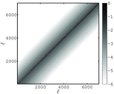
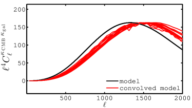
As mentioned before, this procedure is exact only when the $\kappa$ maps are unbiased, such as for lensing simulations. Generally, the optimal mode-mixing matrix involves an additional level of complexity, which arises from the fact that it is not the $\kappa_{\rm gal}$ maps that are masked, but the shear maps, ${\gamma_{1},\gamma_{2}}$. The convergence maps are extracted by performing KS over the masked shear catalogues. The analyses mask are re-applied on the reconstructed $\kappa_{\rm gal}$ maps, but it would be false to assume that there are no other effects. On the contrary, the mask propagates everywhere on the convergence maps. The reconstructed map, $\widetilde{\kappa_{\rm gal}}$, is therefore biased, but can be simply related to the true map in Fourier space (Asgari et al., in prep.):

$$\widetilde{\kappa_{\rm gal}}(\boldsymbol{\ell})=\int\kappa_{\rm gal}(\boldsymbol{\ell}^{\prime})W({\boldsymbol{\ell}}-{\boldsymbol{\ell}^{\prime}})\mbox{d}{\boldsymbol{\ell}^{\prime}}\mbox{cos}2\phi_{\ell\ell^{\prime}}$$ (40)

where $\phi_{\ell\ell^{\prime}}$ is the angle between the vectors ${\boldsymbol{\ell}}$ and ${\boldsymbol{\ell}^{\prime}}$. In the $(\Omega_{L},\eta)$ coordinates introduced above, this angle is exactly $\eta$. When $\kappa$ comes from the masked shear fields, we must replace $\left[\kappa_{\rm gal}W({\boldsymbol{\ell}}-{\boldsymbol{\ell}^{\prime}})\right]$ by $\left[\kappa_{\rm gal}W({\boldsymbol{\ell}}-{\boldsymbol{\ell}^{\prime}})\mbox{cos}2\eta\right]$, which produces an extra factor of $\mbox{cos}2{\eta}$ inside the inner term of equation 33. We are neglecting E/B-mode mixing in this calculation, which is justified since it was shown to be minimal for the CFHTLenS maps in van Waerbeke et al. (2013).

Note that we apply this correction only to the $\kappa_{\rm gal}$ map; correcting the $\kappa_{\rm CMB}$ map requires a modification to the quadratic estimator of Hu & Okamoto (2002), which is beyond the scope of this paper. In addition, this is probably not necessary given the current precision of the CMB lensing maps, which are noise-dominated. In the end, we obtain our optimal mode-mixing matrix by replacing equation 36 with

$$\left\langle W_{1}^{i}(\boldsymbol{L})W^{i*}_{2}(\boldsymbol{L})\right\rangle_{\Omega,\Omega^{\prime}} = 4\pi\!\!\int_{0}^{\pi}\!\!W_{1}^{i}(L)W^{i*}_{2}(L)\mbox{cos}2\eta\mbox{d}\eta$$ (41)

The mode-mixing matrix for pipeline P5 is presented in the upper panel of Fig. 17, in the case of the RCSLenS field CDE2143. Once applied on the theoretical model, this matrix redistributes the power to different $\ell$-modes, as seen in the bottom panel. The forward-modelled predictions are visibly changing from field to field, which needs to be accounted for in a full pseudo-$C_{\ell}$ analysis.

Appendix B Pipeline Comparison

We have shown in Section 6.1 that the choice of analysis pipeline has repercussions on the SNR and on the measured signal. We compare in Fig. 18 the $\hat{C}_{\ell}^{\kappa_{\rm CMB}\kappa_{\rm gal}}$ measurements from RCSLenS, for the 5 pseudo-$C_{\ell}$ pipelines listed in Table 2. Amongst them, P1 has the highest SNR hence is presented in the main body of this paper (Fig. 4). The black squares represent the first data point, $\hat{C}_{\ell=227}^{\kappa_{\rm CMB}\kappa_{\rm gal}}$, measured with methods P1 to P5. The red circles and blue triangles are for $\ell=1015$ and $\ell=1803$ respectively, while the black crosses represent $\hat{C}_{\ell=1803}^{\kappa_{\rm CMB}\kappa_{\rm gal-B}}$, measured from the $\kappa_{\rm gal}$ B-mode maps. Ideally, all points from a given symbol would align horizontally, however we see that it is not the case. They are nevertheless consistent within $1\sigma$, which gives us confidence that our conclusions are relatively insensitive to the choice of pipeline. As future surveys will gain in statistical precision, the error bars on this figure are expected to shrink enough that there will be room for tension across different pipelines. It will therefore be important to reproduce such a validation test to assert the robustness of the measurement.

Figure 18: RCSLenS measurements of the $\hat{C}_{\ell}^{\kappa_{\rm CMB}\kappa_{\rm gal}}$ for all pipelines listed in Table 2. E-modes are presented for multipoles $\ell=227$, 1015 and 1803 in squares, circles and triangles. B-modes are shown for the $\ell=1803$ with cross symbols. All pipelines are consistent within $1\sigma$, however they result in important differences in significance as seen in Table 3.

References

- Allison et al. (2015) Allison, R. et al. 2015, MNRAS, 451, 849
- Asgari et al. (in prep.) Asgari, M., Taylor, A., Kitching, T., & Joachimi, B. in prep.
- Bartelmann & Schneider (2001) Bartelmann, M., & Schneider, P. 2001, Phys. Rep., 340, 291
- Baxter et al. (2016) Baxter, E. J. et al. 2016, ArXiv e-prints, 1602.07384
- Benítez (2000) Benítez, N. 2000, ApJ, 536, 571
- Benjamin et al. (2013) Benjamin, J. et al. 2013, MNRAS, 431, 1547
- Bianchini et al. (2015) Bianchini, F., Lapi, A., & Calabrese, M. e. a. 2015, arXiv, 1511.05116
- Bird et al. (2012) Bird, S., Viel, M., & Haehnelt, M. G. 2012, MNRAS, 420, 2551
- Blake et al. (2015) Blake, C. et al. 2015, ArXiv e-prints, 1507.03086
- Bridle & King (2007) Bridle, S., & King, L. 2007, New Journal of Physics, 9, 444
- Buddendiek & et al. (2015) Buddendiek, A., & et al. 2015, MNRAS, under press
- Chisari et al. (2015) Chisari, N. E., Dunkley, J., Miller, L., & Allison, R. 2015, MNRAS, 453, 682
- Choi et al. (2015) Choi, A. et al. 2015, ArXiv e-prints, 1512.03626
- Coupon et al. (2015) Coupon, J. et al. 2015, MNRAS, 449, 1352
- Das et al. (2014) Das, S. et al. 2014, JCAP, 4, 14
- Demetroullas & Brown (2015) Demetroullas, C., & Brown, M. L. 2015, ArXiv e-prints, 1507.05977
- Erben et al. (2013) Erben, T. et al. 2013, MNRAS, 433, 2545
- Feldman et al. (1994) Feldman, H. A., Kaiser, N., & Peacock, J. A. 1994, ApJ, 426, 23
- Fornengo et al. (2015) Fornengo, N., Perotto, L., Regis, M., & Camera, S. 2015, ApJ, 802, L1
- Giannantonio et al. (2015) Giannantonio, T. et al. 2015, ArXiv e-prints, 1507.05551
- Gilbank et al. (2011) Gilbank, D., Gladders, M., Yee, H., & Hsieh, B. 2011, AJ, 141, 94
- Hall & Taylor (2014) Hall, A., & Taylor, A. 2014, MNRAS, 443, L119
- Hand et al. (2015) Hand, N. et al. 2015, Phys. Rev. D, 91, 062001
- Harnois-Déraps & Pen (2012) Harnois-Déraps, J., & Pen, U.-L. 2012, MNRAS, 423, 2288
- Harnois-Déraps et al. (2013) Harnois-Déraps, J., Pen, U.-L., Iliev, I. T., Merz, H., Emberson, J. D., & Desjacques, V. 2013, MNRAS, 436, 540
- Harnois-Déraps & van Waerbeke (2015) Harnois-Déraps, J., & van Waerbeke, L. 2015, MNRAS, 450, 2857
- Harnois-Déraps et al. (2015) Harnois-Déraps, J., van Waerbeke, L., Viola, M., & Heymans, C. 2015, MNRAS, 450, 1212
- Hartlap et al. (2007) Hartlap, J., Simon, P., & Schneider, P. 2007, A&A, 464, 399
- Heymans et al. (2012) Heymans, C., et al. 2012, MNRAS, 427, 146
- Hildebrandt et al. (2012) Hildebrandt, H. et al. 2012, MNRAS, 421, 2355
- Hildebrandt (in prep.) Hildebrandt, H. e. a. in prep.
- Hill & Spergel (2014) Hill, J. C., & Spergel, D. N. 2014, JCAP, 2, 30
- Hinshaw et al. (2013) Hinshaw, G. et al. 2013, ApJS, 208, 19
- Hivon et al. (2002) Hivon, E., Górski, K. M., Netterfield, C. B., Crill, B. P., Prunet, S., & Hansen, F. 2002, ApJ, 567, 2
- Hojjati et al. (in prep.) Hojjati, A., Tröster, T., van Waerbeke, L., Harnois-Déraps, J., & others. in prep.
- Holder et al. (2013) Holder, G. P. et al. 2013, ApJ, 771, L16
- Hu & Okamoto (2002) Hu, W., & Okamoto, T. 2002, ApJ, 574, 566
- Kaiser & Squires (1993) Kaiser, N., & Squires, G. 1993, ApJ, 404, 441
- Kiessling et al. (2015) Kiessling, A. et al. 2015, Space Sci. Rev., 193, 67
- Kirk et al. (2015a) Kirk, D. et al. 2015a, Space Sci. Rev., 193, 139
- Kirk et al. (2015b) Kirk, D., Omori, Y., Benoit-Lévy, A., Cawthon, R., Chang, C., Larsen, P., & others. 2015b, ArXiv e-prints, 1512.04535
- Kitching et al. (2015a) Kitching, T. D., Heavens, A. F., & Das, S. 2015a, MNRAS, 449, 2205
- Kitching et al. (2008) Kitching, T. D., Miller, L., Heymans, C. E., van Waerbeke, L., & Heavens, A. F. 2008, MNRAS, 390, 149
- Kitching et al. (2015b) Kitching, T. D. et al. 2015b, ArXiv e-prints, 1512.03627
- Kuijken et al. (2015) Kuijken, K. et al. 2015, MNRAS, 454, 3500
- Kuntz (2015) Kuntz, A. 2015, A&A, 584, A53
- Larsen & Challinor (2015) Larsen, P., & Challinor, A. 2015, ArXiv e-prints, 1510.02617
- Lewis et al. (2000) Lewis, A., Challinor, A., & Lasenby, A. 2000, Astrophys. J., 538, 473
- Limber (1954) Limber, D. N. 1954, ApJ, 119, 655
- Liu & Hill (2015) Liu, J., & Hill, J. C. 2015, Phys. Rev. D, 92, 063517
- Liu et al. (2016) Liu, J., Ortiz-Vazquez, A., & Hill, J. C. 2016, ArXiv e-prints, 1601.05720
- Mead et al. (2016) Mead, A., Heymans, C., Lombriser, L., Peacock, J., Steele, O., & Winther, H. 2016, ArXiv e-prints, 1602.02154
- Miller et al. (2013) Miller, L. et al. 2013, MNRAS, 429, 2858
- Miller et al. (2007) Miller, L., Kitching, T. D., Heymans, C., Heavens, A. F., & van Waerbeke, L. 2007, MNRAS, 382, 315
- Miralda-Escude (1991) Miralda-Escude, J. 1991, ApJ, 380, 1
- Moraes et al. (2014) Moraes, B. et al. 2014, in Revista Mexicana de Astronomia y Astrofisica Conference Series, Vol. 44, Revista Mexicana de Astronomia y Astrofisica Conference Series, 202–203
- Moutard et al. (2016) Moutard, T. et al. 2016, ArXiv e-prints, 1602.05917
- Omori & Holder (2015) Omori, Y., & Holder, G. 2015, ArXiv e-prints, 1502.03405
- Planck Collaboration et al. (2015a) Planck Collaboration et al. 2015a, ArXiv e-prints, 1502.05956
- Planck Collaboration et al. (2013) ——. 2013, ArXiv e-prints, 1303.5076
- Planck Collaboration et al. (2014) ——. 2014, A&A, 571, A17
- Planck Collaboration et al. (2015b) ——. 2015b, ArXiv e-prints, 1502.01591
- Schaye et al. (2010) Schaye, J. et al. 2010, MNRAS, 402, 1536
- Scoville et al. (2007) Scoville, N. et al. 2007, ApJS, 172, 1
- Sellentin & Heavens (2016) Sellentin, E., & Heavens, A. F. 2016, MNRAS, 456, L132
- Sherwin et al. (2012) Sherwin, B. D. et al. 2012, Phys. Rev. D, 86, 083006
- Szapudi et al. (2001) Szapudi, I., Prunet, S., Pogosyan, D., Szalay, A. S., & Bond, J. R. 2001, ApJ, 548, L115
- Takahashi et al. (2012) Takahashi, R., Sato, M., Nishimichi, T., Taruya, A., & Oguri, M. 2012, ApJ, 761, 152
- Taylor & Joachimi (2014) Taylor, A., & Joachimi, B. 2014, MNRAS, 442, 2728
- Taylor et al. (2013) Taylor, A., Joachimi, B., & Kitching, T. 2013, MNRAS, 432, 1928
- Troxel & Ishak (2014) Troxel, M., & Ishak, M. 2014, Phys. Rev. D, 89, 063528
- van Daalen et al. (2011) van Daalen, M. P., Schaye, J., Booth, C. M., & Dalla Vecchia, C. 2011, MNRAS, 415, 3649
- van Engelen et al. (2012) van Engelen, A. et al. 2012, ApJ, 756, 142
- van Engelen et al. (2015) ——. 2015, ApJ, 808, 7
- van Waerbeke et al. (2014) van Waerbeke, L., Hinshaw, G., & Murray, N. 2014, Phys. Rev. D, 89, 023508
- van Waerbeke et al. (2013) van Waerbeke, L., et al. 2013, MNRAS, 433, 3373
- Viola et al. (2015) Viola, M. et al. 2015, MNRAS, 452, 3529
- Wall & Jenkins (2003) Wall, J. V., & Jenkins, C. R. 2003, Practical Statistics for Astronomers, ed. R. Ellis, J. Huchra, S. Kahn, G. Rieke, & P. B. Stetson