Going the Distance: Mapping Host Galaxies of LIGO and Virgo Sources in Three Dimensions Using Local Cosmography and Targeted Follow-up

Abstract

The Advanced Laser Interferometer Observatory (LIGO) discovered gravitational waves from a binary black hole merger in 2015 September and may soon observe signals from neutron star mergers. There is considerable interest in searching for their faint and rapidly fading electromagnetic (EM) counterparts, though GW position uncertainties are as coarse as hundreds of square degrees. Since LIGO’s sensitivity to binary neutron stars is limited to the local Universe, the area on the sky that must be searched could be reduced by weighting positions by mass, luminosity, or star formation in nearby galaxies. Since GW observations provide information about luminosity distance, combining the reconstructed volume with positions and redshifts of galaxies could reduce the area even more dramatically. A key missing ingredient has been a rapid GW parameter estimation algorithm that reconstructs the full distribution of sky location and distance. We demonstrate the first such algorithm, which takes under a minute, fast enough to enable immediate electromagnetic follow–up. By combining the three–dimensional posterior with a galaxy catalog, we can reduce the number of galaxies that could conceivably host the event by a factor of 1.4, the total exposure time for the Swift X–ray Telescope by a factor of 2, the total exposure time for a synoptic optical survey by a factor of 2, and the total exposure time for a narrow–field optical telescope by a factor of 3. This encourages us to suggest a new role for small field of view optical instruments in performing targeted searches of the most massive galaxies within the reconstructed volumes.

2016 September 21

=-1

1 Introduction

The Advanced Laser Interferometer Observatory (LIGO; Aasi et al. 2015) began operations in 2015 (Abbott et al., 2016b) and almost immediately recorded the first-ever GW signal from a binary black hole (BBH) merger, GW150914 (Abbott et al., 2016d). It should soon observe GWs from neutron star (NS) binary mergers (Abadie et al., 2010; Abbott et al., 2016f) too. These systems should present several kinds of EM transients that are detectable by existing and planned facilities (e.g., Metzger & Berger 2012). Joint broadband observations would tell the full story of these rare events and solve longstanding puzzles from the nature of short s (SGRBs; Paczynski 1986; Eichler et al. 1989; Narayan et al. 1992; Rezzolla et al. 2011) to the astrophysical sites of $r$-process nucleosynthesis (Rosswog et al. 2014; van de Voort et al. 2015; etc.) and enable these systems to be used as standard siren probes of the evolution history of the universe (Schutz, 1986; Dalal et al., 2006; Nissanke et al., 2010). Metzger & Berger (2012) consider the radioactively powered kilonova (Li & Paczyński, 1998) to be the most promising EM signature to find in coincidence with a LIGO event, though Barnes & Kasen 2013 have shown that the high optical opacities of the ejecta will cause this signature to be faint ($M_{i}\lesssim-13$) and red ($r-i\sim 1$) and to peak quickly, within days to weeks (e.g. Kasen et al. 2015). A consortium of partner gamma-ray, X-rays, optical, and radio facilities have embarked on an unprecedented campaign to search for EM counterparts of GW signals (Abadie et al., 2012b; Evans et al., 2012; Aasi et al., 2014; Abbott et al., 2016c).

GW localizations are currently $\sim 100$–$1000$ deg² (Nissanke et al., 2013; Singer et al., 2014; Berry et al., 2015; Essick et al., 2015) and should shrink to $\sim 10$—$100$ deg² (Abbott et al., 2016e) over years of detector upgrades and construction of additional detectors: Advanced Virgo (Acernese et al., 2015), KAGRA, and LIGO—India. Even the most accurate imaginable GW localizations of $\lesssim$10 deg² will be grossly larger than the $\sim$1$\arcmin$–10$\arcmin$ fields of view of CCD cameras that are common on the world’s largest optical and infrared telescopes. Consequently, robotic and low–overhead synoptic survey telescopes with primary mirror diameters of 1—8 m and FOVs of up to tens of deg² have been heralded as the most promising tools (Metzger & Berger, 2012) for finding those fast and faint EM counterparts.

Kopparapu et al. (2008) and White et al. (2011) recognized that targeting individual galaxies can reduce the area to be searched while eliminating false positive candidates. A galaxy catalog was central to the follow–up strategy during Initial LIGO (Abadie et al., 2012a; Evans et al., 2012; Aasi et al., 2014). Although the increasing number of galaxies within the expanding GW range decreases the utility of this technique, Hanna et al. (2014) and Kasliwal & Nissanke (2014) argued that using both sky positions and distance estimates from GWs can still reduce the number of galaxies, especially in the early years when localizations are particularly coarse. Nissanke et al. (2013) showed that the region bracketed by the upper and lower limits of the 95% credible distance interval can reduce the volume, and hence the number of galaxies, by a factor of 60%.

While the Advanced LIGO commissioning plan calls for several steps in sensitivity and range, parallel construction of additional detectors will result in shrinking sky localization uncertainty (Veitch et al., 2012; Rodriguez et al., 2014). Intriguingly, Gehrels et al. (2016) point out that these effects roughly cancel each other, such that the typical GW error volume may scarcely vary over the next decade.

The obvious next step is to exploit the correlated three–dimensional (3D) structure of the reconstructed volumes. This immediately raises three questions: How accurately can distance be measured with GW detectors, particularly in the early two–detector configurations? What is the 3D shape of the reconstructed volumes? What is the minimal amount of information that is needed to faithfully describe these volumes?

In Singer et al. (2014), we elucidated the localization areas and shapes that we expect in early Advanced LIGO and Virgo. In a similar spirit and using the same catalog of simulated events, we now reveal the shape, scale, and overall character of the 3D reconstructed volumes—enabled by a new and extremely efficient encoding of the 3D probability distributions. We provide a representative sample of GW volume reconstructions in a format that could be made available beginning with the second Advanced LIGO observing run. Complementing existing technologies to detect (Cannon et al., 2012; Messick et al., 2016) and localize (Singer & Price, 2016) GW mergers within minutes of data acquisition, our approach can provide distance-resolved GW sky maps in near real time.

All classes of instruments can benefit from the new 3D localizations, but they are especially powerful for conventional, large-aperture telescopes with narrow-FOV instruments, and particularly at near infrared wavelengths, where large-FOV cameras are scarce (Emerson et al., 2006). Our galaxy-targeted strategy of monitoring the most probable $\sim$100 galaxies for several nights following a GW trigger could be implemented on large infrared facilities. However, even a pilot program on robotic 2 m telescopes could be surprisingly powerful for the first few Advanced LIGO—Virgo observing runs.

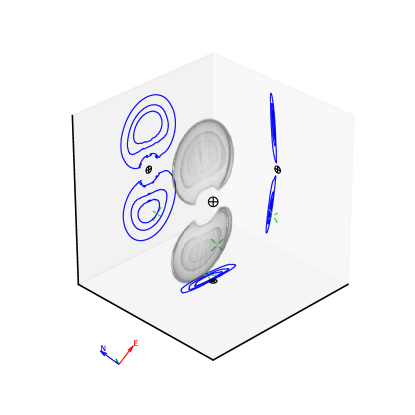
Figure 1: Volume rendering of the 20%, 50%, and 90% credible levels of a typical two-detector early Advanced LIGO event. The three planes are perpendicular to the principal components of the probability distribution. The observer’s position (the Earth) is at the origin. The green reticle shows the true position of the source. The compass in the bottom left corner shows the basis vectors of the equatorial coordinate system.

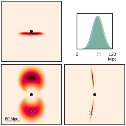
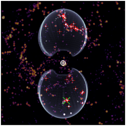
Figure 2: Left panel: marginal posterior probability distribution in the principal planes, as in Fig. 1. The inset shows the marginal distance posterior distribution integrated over the whole sky (blue) and the conditional distance posterior distribution in the true direction of the source (green). Right panel: volume rendering of the 90% credible region superimposed over a slice of the galaxy group map of Tully (2015). The most massive galaxies inside the credible region are highlighted.

2 Distance constraints

The amplitude, or signal–to–noise ratio (S/N), of a GW signal is determined by a degenerate combination of inclination and distance. The Malmquist bias leads to a broad universal distribution of binary inclination angles, peaking at $30\arcdeg$ (Schutz, 2011). The distance of a GW source can generally be estimated with $\sim 30\%$ fractional uncertainty (Cutler & Flanagan, 1994; Berry et al., 2015).

The effective distance $r_{\mathrm{eff}}$ of a GW signal is the maximum distance at which it could have produced the observed S/N. The horizon distance $r_{\mathrm{H}}$ of a detector is the farthest distance at which the most favorably oriented source (at the detector’s zenith, and with a binary inclination of $\iota=0\arcdeg$) would register a threshold S/N (generally defined as $\text{\acs{SNR}}=8$). We give approximate formulae for the horizon distance in Equations (1) and (2) of Singer et al. (2014). The range is the direction- and orientation–averaged distance of sources detectable at a threshold S/N, $r_{\mathrm{R}}\approx r_{\mathrm{H}}/2.26$ (Finn & Chernoff, 1993; Schutz, 2011).

The effective distance description has two major limitations. First, the source may sometimes lie beyond the effective distance because of measurement noise. Worse, there is no obvious way to describe the probability enclosed within, say, the two–dimensional (2D) 90% credible region on the sky and the effective distance; this number is always $\leq 90$%. Second, notwithstanding the large fractional distance uncertainty, there is nontrivial structure to the full 3D reconstructed volumes that can be exploited to reduce the volume under consideration.

During ’s first observing run (O1), the network (Abbott et al., 2016e) consisting of Hanford Observatory (LHO) and Livingston Observatory (LLO) tends to produce probability sky maps consisting of one to two long, thin sections of a great circle (Kasliwal & Nissanke, 2014; Singer et al., 2014). We provide this as an illustration of the main features for a two-detector network. We assume, as in (Abbott et al., 2016e), a B̧NS range of 54 Mpc, though the range during O1 was about 40% better. The corresponding 3D geometry is shown in Figs. 1 and 2. The degenerate arcs correspond to either one or two thin, rounded, slightly oblique petals, about 1$\arcdeg$–5$\arcdeg$ wide, 10$\arcdeg$–100$\arcdeg$ broad, and 10—100 Mpc deep. The “forked tongue” sky localization features due to the degeneracy of the sign of the binary inclination angle (Singer et al., 2014) are evident as narrow crevices running along the outside edges of the petals. The shape irresistibly suggests a tree ear fungus or a seed of the jacaranda tree.

The O2 configuration (Abbott et al., 2016e), which may include LHO and LLO with improved sensitivity at a BNS range of $\sim$100 Mpc, as well as Advanced Virgo, leads to more compact and elaborate combinations of petal-shaped regions. In the most favorable three–detector cases where the area on the sky is localized to a single compact region, the reconstructed volume is a spindle a few degrees in radius and $\sim 100$ Mpc long.

3 Rapid volume reconstruction

Although the reconstructed regions are highly structured, the posterior probability distribution along a given line of sight is simple and generally unimodal; once again, a consequence of the Malmquist bias and the universal distribution of binary inclination angles.

This intuition leads us to suggest that the conditional distribution of distance is well fit by an ansatz whose location parameter $\hat{\mu}(\boldsymbol{n})$, scale $\hat{\sigma}(\boldsymbol{n})$, and normalization $\hat{N}(\boldsymbol{n})$ vary with sky location $\boldsymbol{n}$:

$$p(r|\boldsymbol{n}) =\frac{\hat{N}(\boldsymbol{n})}{\sqrt{2\pi}\hat{\sigma}{(\boldsymbol{n})}}\exp\left[-\frac{\left(r-\hat{\mu}(\boldsymbol{n})\right)^{2}}{2\hat{\sigma}(\boldsymbol{n})^{2}}\right]r^{2}$$ (1)

$$\text{for }r \geq 0.$$

This form is equivalent to the product of a Gaussian likelihood and a uniform-in-volume prior. We show that this is a good fit in Section 6 of the Supplement.

The outputs of the LIGO—Virgo localization pipelines are HEALPix (Hierarchical Equal Area isoLatitude Pixelization) all–sky images whose $N_{\mathrm{pix}}$ pixels give the posterior probability $\rho_{i}$ that the source is contained inside pixel $i$. We add three additional layers: $\hat{\mu}_{i}=\hat{\mu}(\boldsymbol{n}_{i})$, $\hat{\sigma}_{i}=\hat{\sigma}(\boldsymbol{n}_{i})$, and (for convenience) $\hat{N}_{i}=\hat{N}(\boldsymbol{n}_{i})$. The first layer, $\rho_{i}$, is unchanged and still represents the 2D probability sky map.

The probability that a source is within pixel $i$ and at a distance between $r$ and $r+dr$ is $\rho_{i}$ times Eq. (1):

$$P(r,\boldsymbol{n}_{i})\,dr=\rho_{i}\frac{\hat{N}_{i}}{\sqrt{2\pi}\hat{\sigma}_{i}}\exp\left[-\frac{\left(r-\hat{\mu}_{i}\right)^{2}}{2{\hat{\sigma}_{i}}^{2}}\right]r^{2}\,dr.$$ (2)

The sky map is normalized such that

$$\sum_{i\,=\,0}^{N-1}\rho_{i}=1,$$ (3)

so Eq. (2) is also normalized such that

$$\sum_{i\,=\,0}^{N-1}\int_{0}^{\infty}P(r,\boldsymbol{n}_{i})\,dr=1.$$ (4)

The $r^{2}$ term is necessary in Eqs. (1, 2) so that the probability density per unit volume vanishes at the origin. Eq. (2) should be thought of as the probability distribution in spherical polar coordinates. If, however, one needs to perform a calculation in Cartesian coordinates, one converts using volume element, given by

$$dV=r^{2}\,dr\,\Delta\Omega=\frac{4\pi}{N_{\mathrm{pix}}}r^{2}\,dr.$$ (5)

The $r^{2}$ cancels in the resulting probability density per unit volume:

$$\frac{dP}{dV}=\rho_{i}\frac{N_{\mathrm{pix}}}{4\pi}\frac{\hat{N}_{i}}{\sqrt{2\pi}\hat{\sigma}_{i}}\exp\left[-\frac{\left(r-\hat{\mu}_{i}\right)^{2}}{2{\hat{\sigma}_{i}}^{2}}\right].$$ (6)

Sky maps for compact binary merger candidates are produced by two codes with complementary sophistication and speed. The first is BAYESTAR, which rapidly triangulates matched–filter estimates of the times, amplitudes, and phases on arrival at the GW sites (Singer & Price, 2016). The second is LALInference, which stochastically samples from sky location, distance, and component masses and spins (Veitch et al., 2015). Both methods directly sample the full 3D posterior probability distribution. The ansatz parameters are extracted using the method of moments as elaborated upon in Section 5 of the Supplement.

4 Implications for early Advanced LIGO and Virgo

We use this encoding to demonstrate the utility of the 3D structure of the GW posteriors. LIGO provided 2D localizations during O1 but did not calculate or distribute low-latency GW distance estimates. (A directional distance estimate for GW151226 produced two weeks after the event (LSC & Virgo 2016; Smartt et al. 2016) did help to rule out the redshift of a Pan-STARRS optical transient candidate.) Without a 3D sky map, one could have provided the horizon distance $r_{\mathrm{H}}$ calculated from the detectors’ sensitivity or the effective distance $r_{\mathrm{eff}}$ based on the signal’s S/N. The new 3D sky maps allow us to find 90% credible volumes that are 2–30 times smaller (10th to 90th percentile) than the volume within the 2D 90% credible area and the horizon distance, or 1–7 times smaller than the volume within the 2D 90% credible area and the effective distance.

However, the 3D localizations truly shine when we minimize not the volume, but rather the total exposure time required to observe every galaxy within the 90% credible volume to a given flux limit. We neglect intrinsic scatter in absolute magnitude; the resulting conservative figure of merit allows us to focus on the effect of the distance posterior itself.

If BNS mergers have hosts that are similar to short s, then their local rates are likely traced by a combination of recent star formation (measured by $B$-band luminosity) and stellar mass (measured by $K$-band luminosity; e.g. Leibler & Berger 2010; Fong et al. 2013). As in Gehrels et al. (2016), we attempt to mitigate these concerns as the limited completeness of galaxy catalogs by considering only the brightest galaxies. If we assume a $B$–band Schechter function with $\alpha=-1.25$, $\phi^{*}=1.2\times 10^{-2}$ $h^{3}$ Mpc^-3, and $L^{*}=1.2\times 10^{10}$ $h^{-2}$ $L_{\odot}$ (Longair, 2008) as a proxy for the BNS merger rate, then we find that $2.8\times 10^{-3}$ galaxies per Mpc³ comprise half of the total luminosity (see Fig. 3). The areal density of galaxies out to a distance $r$ and with a luminosity greater than $L$ is

$$N_{\mathrm{gal}}\approx 0.28\text{ deg}^{-2}\\ \left(\frac{r}{100\text{ Mpc}}\right)^{3}\left(\frac{\phi^{*}}{4\times 10^{-3}\text{ Mpc}^{-3}}\right)\Gamma\left(\alpha+1,\frac{L}{L^{*}}\right),$$ (7)

at most a handful per deg² within distances that are relevant for BNS mergers.

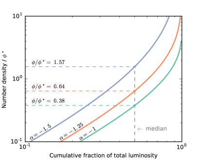
Figure 3: Tradeoff between completeness and the number of galaxies, assuming various Schechter luminosity functions. The horizontal axis is the cumulative fraction of the total luminosity in the local Universe. The vertical axis is the number density of galaxies in units of $\phi^{*}$.

As a proof of concept, in the right panel of Fig. 2, we show the potential host galaxies that are consistent with a simulated early Advanced LIGO BNS localization. We use the galaxy group catalog of Tully (2015). This may not be an ideal galaxy catalog for GW follow-up; among other reasons, being derived from 2MASS, its magnitudes trace mass rather than recent star formation. Better alternatives that should be available in the near future include the Census of the Local Universe (D. Cook et al. 2016, in preparation; Gehrels et al. 2016) and the Galaxy List for the Advanced Detector Era. However, pending the availability of larger compilations of galaxy catalogs, it serves to illustrate our idea because it is $\sim∼$50% complete out to $\sim 150$ Mpc. Furthermore, incompleteness is encoded self-consistently by placing a variable bandwidth weighted kernel at the position of each galaxy.

Our control observing strategy takes all galaxies within a given 2D credible region, out to an optimal direction-independent distance inferred from the estimated mass of the source, the loudness of the signal, and the sensitivity of the detectors. It employs the same exposure time for every galaxy. This naive 2+1—dimensional (2+1D) construction is already far more sophisticated than the effective distance or horizon distance that could have been available in O1.

Different facilities demand different figures of merit. For FOVs $\ll 0.5\text{ deg}^{2}$, most observations pick out single galaxies. In this case, the optimal selection of galaxies exploits both the upper and lower limits of the reconstructed volume, and the total exposure time is dependent on the number density of galaxies. For FOVs $\gg 0.5\text{ deg}^{2}$, most observations pick out many galaxies; an exposure tuned to reach a fixed luminosity limit for a distant galaxy also captures all of the galaxies at intervening distances. In this case, we tune the exposure time to reach the most distant galaxy in each field, and the total exposure time is independent of the number density of galaxies. The instrument sensitivity is also important. In the source limited regime, the exposure time to reach a fixed limiting luminosity for a source at a distance $r$ varies as $r^{2}$. For sky background limited imaging, the time scales as $r^{4}$. The three cases of greatest interest are summarized below:

$$T=\min_{D:\int\limits_{D}P\,dV\,=\,0.9}\begin{cases}\displaystyle\frac{T^{*}}{\omega}\displaystyle\int_{D}\left(\frac{r}{r^{*}}\right)^{4}d\Omega&\begin{subarray}{c}\displaystyle{\text{\emph{I}: large \acs{FOV},}}\\ \displaystyle{\text{sky limited}}\end{subarray}\\[8.61108pt] T^{*}\phi\displaystyle\int_{D}\left(\frac{r}{r^{*}}\right)^{2}dV&\begin{subarray}{c}\displaystyle{\text{\emph{II}: small \acs{FOV},}}\\ \displaystyle{\text{source limited}}\end{subarray}\\[8.61108pt] T^{*}\phi\displaystyle\int_{D}\left(\frac{r}{r^{*}}\right)^{4}dV&\begin{subarray}{c}\displaystyle{\text{\emph{III}: small \acs{FOV},}}\\ \displaystyle{\text{sky limited}.}\end{subarray}\end{cases}$$ (8)

Here, $T^{*}$ is the time required to reach a fiducial flux limit for a source at a distance $r^{*}$, $\phi$ is the average number density of galaxies, and $\omega$ is the FOV of the instrument in steradians. The integral is over solid angle (case I) or volume (cases II and III) and is minimized over all possible regions $D$ that contain 90% posterior probability. Table 1 presents the results of this exercise: volumes, numbers of galaxies, and exposure times. Each case typifies a search for a different EM signature with a different kind of instrument:

Case I

describes a kilonova search with a synoptic optical survey instrument. We adopt the Zwicky Transient Facility (ZTF) our example and assume a FOV of 47 deg². Adopting $M_{i}=-13$ as the absolute magnitude of a kilonova, we derive from Table 1 of Kasliwal & Nissanke (2014) a fiducial ZTF exposure time of $T^{*}\approx 6600$ s for a limiting magnitude of $i\approx 23.5$ at a distance of $r^{*}=200$ Mpc. In O1, a ZTF–like survey would have taken $\sim$0.4 hr to tile the entire region to an appropriate depth in exposures that average $\sim$2 minutes in duration. The number of exposures decreases to a handful in the HLV configuration in ’s second observing run (O2), but the exposure duration increases to 35 minutes per field.

Case II

models an afterglow search with the Swift X–ray Telescope (XRT) (considered in detail by Evans et al. 2016). Following Kanner et al. (2012), we adopt a fiducial exposure time of $T^{*}=100$ s at $r^{*}=200$ Mpc. In O1, we find an average exposure time of 7 s per field, increasing to 25 s per field in O2. These are unrealistically short due to Swift’s slew rate ($3\arcdeg$ s^-1) and overhead (25 s; Evans et al. 2016). However, even adding an overhead of $\sim$30 s per galaxy, we suggest that a galaxy–targeted Swift campaign could be accomplished within a few 90 minute orbits.

Case III

describes a kilonova search with a traditional small FOV optical telescope. Since we need to examine tens to hundreds of galaxies, we restrict ourselves to fully robotic telescopes dedicated to time–domain science and select the Las Cumbres Observatory Global Telescope (LCOGT) and Liverpool 2 m telescopes as our models. Using the LCOGT exposure time calculator, we find an exposure time of $T^{*}\approx 2500$ s to reach a depth of $i=23.5$ mag at $\text{\acs{SNR}}=5$ during half moon phase on the Spectral camera. In O1 we find an average exposure time of about 0.2 minute, for a total exposure time of 0.4 hr. Overhead would dominate. The average exposure time increases to $\sim$2.5 minutes in O2. The total exposure time increases dramatically from 0.4 to over 13.4 hr due to the rapid increase in exposure time with distance and the modest increase in the number of galaxies. However, the total exposure time is still short enough that two 2 m telescopes working in coordination could conceivably monitor all of the selected galaxies at a 1—2 night cadence.

Table 1: Median Volumes and Exposure Times

			Range					Large FOV/Sky			Small FOV/Source			Small FOV/Sky
			(Mpc)		Vol. ($10^{3}$	No.		Ex.: ZTF			Ex.: Swift XRT			Ex.: LCOGT 2 m
Run	Year	Net.	HL	V	Mpc3)	Gal.	Red.	Tot.	Avg.	Red.	Tot.	Avg.	Red.	Tot.	Avg.	Red.
O1	2015	HL	54	—	29	80	0.62	0.4	2	0.41	0.2	0.1	0.46	0.4	0.2	0.35
O2	2016	HL	108	—	324	906	0.59	6.9	23	0.38	6.9	0.4	0.42	56.2	2.6	0.31
		HLV	108	36	56	156	0.75	1.5	35	0.52	1.5	0.4	0.58	13.4	2.5	0.43

5 Discussion

To order to focus on the utility of distance and structure information, we neglected several details. Chen & Holz (2014) address optimal selection of which GW events to follow up. We set aside the feasibility of imaging tens to hundreds of targets in rapid succession with Swift, though this is being implemented (Evans et al., 2016). We ignored the question of whether the XRT exposure time can be finely tuned from one target to the next, though our results justify doing so if possible. We ignored variation in observability conditions such as Sun and Earth avoidance, weather, South Atlantic Anomaly passages, and Moon phase, details which are better left to a facility–specific paper. We did not consider optimizing field selection given limited time resources, for which we refer the reader to Chan et al. (2015).

We did not address the significant issues of galaxy catalog completeness, construction of a galaxy prior from an incomplete galaxy catalog (Fan et al., 2014), or the suitability of any particular galaxy catalog, though targeting the brightest and most massive galaxies (those with $L\gtrsim L^{*}$) should simplify these concerns (Gehrels et al., 2016).

Antolini & Heyl (2016) proposed using photometric redshifts to optimize GW follow-up, improving completeness at the expense of accurate distances. Improved completeness mitigates the concern that BBH mergers like GW150914, which are probably formed in low-metallicity environments (Abbott et al., 2016a), may display host environment preferences similar to long gamma-ray bursts and probably do not track with massive galaxies. However, our present work focuses on NS binary mergers, which are expected to be found in fairly eclectic host environments due to the long time delay between formation and evolution of the binary and its GW-driven inspiral into the LIGO band. Therefore, the completeness of existing spectroscopic redshift surveys seems tolerable for our approach and for BNSs.

One possible concern for small-FOV telescopes is the offsets that mergers may have from their host galaxies due to supernova (SN) kicks. Fong & Berger (2013) find that SGRBs have a median offsets of 4.5 kpc from their hosts. For even an improbably nearby merger at $z=0.005$ or a luminosity distance $r=22$ Mpc, the projected radius of the $24\arcmin$ XRT FOV is 74 kpc, and of the $10\arcmin$ LCOGT imager, 31 kpc, encapsulating well over 90% of SGRB offsets.

In principal, our exposure time estimates should account not only for sky background, but additional image subtraction background due to the light of the host galaxy. Offsets should help here too because SGRBs are typically found at separations $>1.5$ times the effective radii of their host galaxies.

One particular advantage of galaxy-targeted searches is the reduction in false positives. In a magnitude-limited snapshot, SNe of Types Ia, Ibc, and II are found in proportions of 68.6%:4.3%:27.1% (Li et al., 2011). Assuming a volumetric rate of $3\times 10^{-5}$ Mpc^-3 yr^-1 (Li et al., 2011), an average absolute magnitude of $-19$ over a duration of 1 week, and a limiting magnitude of 23.5, we calculate an areal rate of about 2 Type Ia SNe per deg². A typical wide–field GW follow–up campaign searching an area of $\sim 100$ deg² will be contaminated by hundreds of SNe. However, if we consider only $10\arcmin\times 10\arcmin$ patches around 100 nearby galaxies, the on–sky footprint of $<$3 deg² translates to a background of merely 6 SNe Ia and 3 core-collapse SNe.

This points toward a new role in GW follow–up for small-FOV, large-aperture telescopes, in addition to and beyond their role of vetting candidates identified by synoptic surveys. Setting aside scheduling and proposal processes for the time being, suitable facilities for our strategy should have primary mirror diameters of 4–10 m and optical or infrared imagers with $\sim 10\arcmin$ FOVs that are either permanently installed at one of the foci or are rapidly deployable (e.g., mounted on Nasmyth platforms). Candidates include ALFOSC on the Nordic Optical Telescope, LMI on the Discovery Channel Telescope, WIRC on the Hale Telescope at Palomar, FourStar on Magellan, GMOS on Gemini North and South, FLAMINGOS-2 on Gemini South, FORS2 on VLT, LRIS at Keck, or GTC equipped with OSIRIS. As a pathfinder, we encourage deploying existing 2 m class robotic optical telescopes in this manner during the early Advanced LIGO and Virgo observing runs.

2D

two–dimensional

2+1D

2+1—dimensional

2MRS

2MASS Redshift Survey

3D

three–dimensional

2MASS

Two Micron All Sky Survey

AdVirgo

Advanced Virgo

AMI

Arcminute Microkelvin Imager

AGN

active galactic nucleus

aLIGO

Advanced LIGO

ASKAP

Australian Square Kilometer Array Pathfinder

ATCA

Australia Telescope Compact Array

ATLAS

Asteroid Terrestrial-impact Last Alert System

BAT

Burst Alert Telescope (instrument on Swift)

BATSE

Burst and Transient Source Experiment (instrument on CGRO)

BAYESTAR

BAYESian TriAngulation and Rapid localization

BBH

binary black hole

BHBH

black hole—black hole

BH

black hole

BNS

binary neutron star

CARMA

Combined Array for Research in Millimeter–wave Astronomy

CASA

Common Astronomy Software Applications

CFH12k

Canada–France–Hawaii $12\,288\times 8\,192$ pixel CCD mosaic (instrument formerly on the Canada–France–Hawaii Telescope, now on the Palomar 48 inch Oschin telescope (P48))

CRTS

Catalina Real-time Transient Survey

CTIO

Cerro Tololo Inter-American Observatory

CBC

compact binary coalescence

CCD

charge coupled device

CDF

cumulative distribution function

CGRO

Compton Gamma Ray Observatory

CMB

cosmic microwave background

CRLB

Cramér—Rao lower bound

cWB

Coherent WaveBurst

DASWG

Data Analysis Software Working Group

DBSP

Double Spectrograph (instrument on P200)

DCT

Discovery Channel Telescope

DECam

Dark Energy Camera (instrument on the Blanco 4–m telescope at CTIO)

DES

Dark Energy Survey

DFT

discrete Fourier transform

EM

electromagnetic

ER8

eighth engineering run

FD

frequency domain

FAR

false alarm rate

FFT

fast Fourier transform

FIR

finite impulse response

FITS

Flexible Image Transport System

FLOPS

floating point operations per second

FOV

field of view

FTN

Faulkes Telescope North

FWHM

full width at half-maximum

GBM

Gamma-ray Burst Monitor (instrument on Fermi)

GCN

Gamma-ray Coordinates Network

GMOS

Gemini Multi-object Spectrograph (instrument on the Gemini telescopes)

GRB

gamma-ray burst

GSC

Gas Slit Camera

GSL

GNU Scientific Library

GTC

Gran Telescopio Canarias

GW

gravitational wave

HAWC

High–Altitude Water Čerenkov Gamma–Ray Observatory

HCT

Himalayan Chandra Telescope

HEALPix

Hierarchical Equal Area isoLatitude Pixelization

HEASARC

High Energy Astrophysics Science Archive Research Center

HETE

High Energy Transient Explorer

HFOSC

Himalaya Faint Object Spectrograph and Camera (instrument on HCT)

HMXB

high–mass X–ray binary

HSC

Hyper Suprime–Cam (instrument on the 8.2–m Subaru telescope)

IACT

imaging atmospheric Čerenkov telescope

IIR

infinite impulse response

IMACS

Inamori-Magellan Areal Camera & Spectrograph (instrument on the Magellan Baade telescope)

IMR

inspiral-merger-ringdown

IPAC

Infrared Processing and Analysis Center

IPN

InterPlanetary Network

iPTF

intermediate Palomar Transient Factory

ISM

interstellar medium

ISS

International Space Station

KAGRA

KAmioka GRAvitational–wave observatory

KDE

kernel density estimator

KN

kilonova

LAT

Large Area Telescope

LCOGT

Las Cumbres Observatory Global Telescope

LHO

LIGO Hanford Observatory

LIB

LALInference Burst

LIGO

Laser Interferometer GW Observatory

llGRB

low–luminosity GRB

LLOID

Low Latency Online Inspiral Detection

LLO

LIGO Livingston Observatory

LMI

Large Monolithic Imager (instrument on Discovery Channel Telescope (DCT))

LOFAR

Low Frequency Array

LOS

line of sight

LMC

Large Magellanic Cloud

LSB

long, soft burst

LSC

LIGO Scientific Collaboration

LSO

last stable orbit

LSST

Large Synoptic Survey Telescope

LT

Liverpool Telescope

LTI

linear time invariant

MAP

maximum a posteriori

MBTA

Multi-Band Template Analysis

MCMC

Markov chain Monte Carlo

MLE

maximum likelihood (ML) estimator

ML

maximum likelihood

MOU

memorandum of understanding

MWA

Murchison Widefield Array

NED

NASA/IPAC Extragalactic Database

NSBH

neutron star—black hole

NSBH

neutron star—black hole

NSF

National Science Foundation

NSNS

neutron star—neutron star

NS

neutron star

O1

Advanced ’s first observing run

O2

Advanced ’s second observing run

oLIB

Omicron+LALInference Burst

OT

optical transient

P48

Palomar 48 inch Oschin telescope

P60

robotic Palomar 60 inch telescope

P200

Palomar 200 inch Hale telescope

PC

photon counting

PESSTO

Public ESO Spectroscopic Survey of Transient Objects

PSD

power spectral density

PSF

point-spread function

PS1

Pan–STARRS 1

PTF

Palomar Transient Factory

QUEST

Quasar Equatorial Survey Team

RAPTOR

Rapid Telescopes for Optical Response

REU

Research Experiences for Undergraduates

RMS

root mean square

ROTSE

Robotic Optical Transient Search

S5

LIGO’s fifth science run

S6

LIGO’s sixth science run

SAA

South Atlantic Anomaly

SHB

short, hard burst

SHGRB

short, hard gamma-ray burst

SKA

Square Kilometer Array

SMT

Slewing Mirror Telescope (instrument on UFFO Pathfinder)

S/N

signal–to–noise ratio

SSC

synchrotron self–Compton

SDSS

Sloan Digital Sky Survey

SED

spectral energy distribution

SGRB

short gamma-ray burst

SN

supernova

SN Ia

Type Ia SN

SN Ic–BL

broad–line Type Ic SN

SVD

singular value decomposition

TAROT

Télescopes à Action Rapide pour les Objets Transitoires

TDOA

time delay on arrival

TD

time domain

TOA

time of arrival

TOO

target–of–opportunity

UFFO

Ultra Fast Flash Observatory

UHE

ultra high energy

UVOT

UV/Optical Telescope (instrument on Swift)

VHE

very high energy

VISTA@ESO

Visible and Infrared Survey Telescope

VLA

Karl G. Jansky Very Large Array

VLT

Very Large Telescope

VST@ESO

VLT Survey Telescope

WAM

Wide–band All–sky Monitor (instrument on Suzaku)

WCS

World Coordinate System

w.s.s.

wide–sense stationary

XRF

X–ray flash

XRT

X–ray Telescope (instrument on Swift)

ZTF

Zwicky Transient Facility

References

- Aasi et al. (2014) Aasi, J., Abadie, J., Abbott, B. P., et al. 2014, ApJS, 211, 7
- Aasi et al. (2015) —. 2015, CQGra, 32, 074001
- Abadie et al. (2010) Abadie, J., Abbott, B. P., Abbott, R., et al. 2010, CQGra, 27, 173001
- Abadie et al. (2012a) —. 2012a, A&A, 541, A155
- Abadie et al. (2012b) —. 2012b, A&A, 539, A124
- Abbott et al. (2016a) Abbott, B. P., Abbott, R., Abbott, T. D., et al. 2016a, ApJ, 818, L22
- Abbott et al. (2016b) —. 2016b, Phys. Rev. Lett., 116, 131103
- Abbott et al. (2016c) —. 2016c, ApJ, 826, L13
- Abbott et al. (2016d) —. 2016d, Phys. Rev. Lett., 116, 061102
- Abbott et al. (2016e) —. 2016e, Living Reviews in Relativity, 19, arXiv:1304.0670
- Abbott et al. (2016f) —. 2016f, arXiv:1607.07456
- Acernese et al. (2015) Acernese, F., Agathos, M., Agatsuma, K., et al. 2015, CQGra, 32, 024001
- Antolini & Heyl (2016) Antolini, E., & Heyl, J. S. 2016, arXiv:1602.07710
- Barnes & Kasen (2013) Barnes, J., & Kasen, D. 2013, ApJ, 775, 18
- Berry et al. (2015) Berry, C. P. L., Mandel, I., Middleton, H., et al. 2015, ApJ, 804, 114
- Cannon et al. (2012) Cannon, K., Cariou, R., Chapman, A., et al. 2012, ApJ, 748, 136
- Chan et al. (2015) Chan, M. L., Hu, Y.-M., Messenger, C., Hendry, M., & Heng, I. S. 2015, arXiv:1506.04035
- Chen & Holz (2014) Chen, H.-Y., & Holz, D. E. 2014, arXiv:1409.0522
- Cutler & Flanagan (1994) Cutler, C., & Flanagan, É. E. 1994, Phys. Rev. D, 49, 2658
- Dalal et al. (2006) Dalal, N., Holz, D. E., Hughes, S. A., & Jain, B. 2006, Phys. Rev. D, 74, 063006
- Eichler et al. (1989) Eichler, D., Livio, M., Piran, T., & Schramm, D. N. 1989, Nature, 340, 126
- Emerson et al. (2006) Emerson, J., McPherson, A., & Sutherland, W. 2006, Msngr, 126, 41
- Essick et al. (2015) Essick, R., Vitale, S., Katsavounidis, E., Vedovato, G., & Klimenko, S. 2015, ApJ, 800, 81
- Evans et al. (2012) Evans, P. A., Fridriksson, J. K., Gehrels, N., et al. 2012, ApJS, 203, 28
- Evans et al. (2016) Evans, P. A., Osborne, J. P., Kennea, J. A., et al. 2016, MNRAS, 455, 1522
- Fan et al. (2014) Fan, X., Messenger, C., & Heng, I. S. 2014, ApJ, 795, 43
- Finn & Chernoff (1993) Finn, L. S., & Chernoff, D. F. 1993, Phys. Rev. D, 47, 2198
- Fong & Berger (2013) Fong, W., & Berger, E. 2013, ApJ, 776, 18
- Fong et al. (2013) Fong, W., Berger, E., Chornock, R., et al. 2013, ApJ, 769, 56
- Gehrels et al. (2016) Gehrels, N., Cannizzo, J. K., Kanner, J., et al. 2016, ApJ, 820, 136
- Hanna et al. (2014) Hanna, C., Mandel, I., & Vousden, W. 2014, ApJ, 784, 8
- Kanner et al. (2012) Kanner, J., Camp, J., Racusin, J., Gehrels, N., & White, D. 2012, ApJ, 759, 22
- Kasen et al. (2015) Kasen, D., Fernández, R., & Metzger, B. D. 2015, MNRAS, 450, 1777
- Kasliwal & Nissanke (2014) Kasliwal, M. M., & Nissanke, S. 2014, ApJ, 789, L5
- Kopparapu et al. (2008) Kopparapu, R. K., Hanna, C., Kalogera, V., et al. 2008, ApJ, 675, 1459
- Leibler & Berger (2010) Leibler, C. N., & Berger, E. 2010, ApJ, 725, 1202
- Li & Paczyński (1998) Li, L.-X., & Paczyński, B. 1998, ApJ, 507, L59
- Li et al. (2011) Li, W., Leaman, J., Chornock, R., et al. 2011, MNRAS, 412, 1441