From four- to two-channel Kondo effect in junctions of XY spin chains

Abstract

We consider the Kondo effect in $Y$-junctions of anisotropic $XY$ models in an applied magnetic field along the critical lines characterized by a gapless excitation spectrum. We find that, while the boundary interaction Hamiltonian describing the junction can be recasted in the form of a four-channel, spin-$1/2$ antiferromagnetic Kondo Hamiltonian, the number of channels effectively participating in the Kondo effect depends on the chain parameters, as well as on the boundary couplings at the junction. The system evolves from an effective four-channel topological Kondo effect for a junction of $XX$-chains with symmetric boundary couplings into a two-channel one at a junction of three quantum critical Ising chains. The effective number of Kondo channels depends on the properties of the boundary and of the bulk. The $XX$-line is a ”critical” line, where a four-channel topological Kondo effect can be recovered by fine-tuning the boundary parameter, while along the line in parameter space connecting the $XX$-line and the critical Ising point the junction is effectively equivalent to a two-channel topological Kondo Hamiltonian. Using a renormalization group approach, we determine the flow of the boundary couplings, which allows us to define and estimate the critical couplings and Kondo temperatures of the different Kondo (pair) channels. Finally, we study the local transverse magnetization in the center of the $Y$-junction, eventually arguing that it provides an effective tool to monitor the onset of the two-channel Kondo effect.

1 Introduction

The Kondo effect arises from the interaction between magnetic impurities and itinerant electrons in a metal, resulting in a net low-temperature increase of the resistance [1, 2, 3]. Due to the large amount of analytical and numerical tools developed to attack it and to its relevance for a variety of systems including heavy fermion materials [2], it became a paradigmatic example of a strongly interacting system and a testing ground for new many-body techniques.

The Kondo effect has been initially studied for metals, like copper, in which magnetic atoms, like cobalt, are added. However, the interest in the Kondo physics persisted also because it is possible to realize it in a controlled way in devices such as, for instance, quantum dots [4, 5]. Indeed, when an odd number of electrons is trapped within the dot, it effectively behaves as a spin-1/2 localized magnetic impurity: such a localized spin, placed between two leads, mimics a magnetic impurity in a metal.

Another class of physical systems proposed to host the Kondo physics is provided by quantum spin chains [6, 7, 8]: the rationale is that the electron Kondo problem may be described by a one-dimensional model since only the $s$-wave part of the electronic wavefunction is affected by the Kondo coupling. In [8] a magnetic impurity (i.e. an extra spin) at the end of a $J_{1}-J_{2}$ spin chain was studied and the comparison between the usual free electron Kondo model and this spin chain version was discussed: it was found that in general in the spin chain Kondo model a marginally irrelevant bulk interaction may be present, whose coupling in the $J_{1}-J_{2}$ model can be tuned to zero by choosing $J_{2}$ at the critical value of the gapless/dimerized phase transition. However, apart from the possible presence of these marginal interactions modifying the details of the flow to the strong coupling Kondo fixed point, the results indicate that the behavior is qualitatively the same as in the standard Kondo effect [8, 9, 10, 11, 12, 13, 14, 15, 16]. Moreover, it was also pointed out that a remarkable realization of the overscreened two-channel Kondo effect can be realized with two impurities in the $J_{1}-J_{2}$ chain [10, 11, 13, 16].

An important advantage of using spin chains to simulate magnetic impurities is that they provide in a natural way the possibility of nontrivially tuning the properties of the corresponding low-energy effective Kondo Hamiltonian and to engineer in a controllable way the impurity and its coupling to the bulk degrees of freedom. A recent paradigmatic example in this direction is provided by $Y$-junctions of suitably chosen spin chains [17, 18]. This kind of $Y$-junction is obtained when several (say, $M$) spin chains (the ”bulk”) are coupled to each other through a ”central region” (the ”boundary”). For instance, one can couple the chains by connecting the initial spins of each chain with each other with certain boundary couplings possibly different from the bulk ones.

Models of $Y$-junctions have been studied at the crossing, or the coupling, of three, or more, Luttinger liquids [19, 20, 21, 22, 23, 24, 25, 26], in Bose gases in star geometries [27, 28, 29], and in superconducting Josephson junctions [22, 30]. Along this last direction, it has also been proposed to simulate the two-channel Kondo effect at a $Y$-junction of quantum Ising chains [18] or in a pertinently designed Josephson junction network [31]. A related system, a junction of $M$ classical two-dimensional Ising models, has been studied in [32], where it was discussed the surface critical behavior, showing in particular that the $M\to 0$ limit corresponds to the semi-infinite Ising model in the presence of a random surface field.

In a $Y$-junction it is actually the coupling among bulk chains that determines the magnetic impurity. Formally, this arises from the extension of the standard Jordan-Wigner (JW) transformation [33] to the non-ordered manifold provided by the junction of three (or more) chains [17]. In order to preserve the correct (anti)commutation relations, this requires adding ancillary degrees of freedom associated to the central region, which is a triangle for $M=3$: after this JW transformation, that requires the introduction of appropriate Klein factors [17], the additional variables determine a spin variable magnetically coupled with the JW fermions from the chains which is topological, in view of the nonlocal character of the auxiliary fermionic variables [34], realized as real-fermion Klein factors. On implementing this procedure in the case of a junction of three Ising chains in a transverse field tuned at their quantum critical point, one recovers a realization of the two-channel topological Kondo model [18]. At variance, if one applies the procedure to a junction of three $XX$ chains, then one obtains a realization of the four-channel topological Kondo model [17]. In general, a reason of interest in studying such $Y$-junctions of spin chains is that it provides a remarkable physical realization of the topological Kondo effect [34, 35, 36, 37, 38, 39, 40].

In general, a tunable effective Kondo Hamiltonian can be realized at a $Y$-junction of quantum spin chains, provided the following requirements are met:

1. Of course, the spin chains should have tunable parameters; the solvability of the model on the chain is not strictly requested, but it helps in identifying the correct mapping between the $Y$-junction of spin chains and the Kondo Hamiltonian;

2. The bulk Hamiltonian in the chains should be gapless (which is the case of the critical Ising model in a transverse field [18] and of the $XX$ model [17]). Even though the study of boundary effects in $Y$-junctions of gapped chains may be interesting in its own, because of the competition between the scales given by the Kondo length and by the correlation length associated to the bulk gap (similar to what happens for magnetic impurities in a superconductor [41], for the Josephson current in a junction containing resonant impurity levels [42] or for a quantum dot coupled to two superconductors [43, 44, 45]), yet, strictly speaking, in the case of a gapped bulk spectrum one does not recover a Kondo fixed point.

The $XY$ model in a transverse field which we consider in this paper meets both the above requirements in one shot, since:

• It is solvable for the uncoupled chains via JW transformations [46, 47, 48];

• It has two free parameters, the transverse field $H$ and the anisotropy $\gamma$ (in fact, the magnetic coupling $J$ can be just regarded as an over-all energy scale);

• Taken in pertinent limits, it reduces both to the $XX$ model ($\gamma=1$, $H=0$) and to the critical Ising model ($\gamma=0$, $H=2J$);

• Last, but essential for our purposes, the parameters $H$ and $J$ can be chosen in a way that one can interpolate between the two limits, $XX$ and critical Ising, keeping a gapless bulk excitation spectrum.

After performing the JW transformation in the bulk and introducing the additional (”topological spin”) degrees of freedom at the junction, it has been established in [17] that a junction of three quantum $XX$-chains hosts a spin-chain realization of the four-channel Kondo effect (4CK). At variance, in [18] it has been shown that a junction of three critical quantum Ising chains can be mapped onto a two-channel Kondo (2CK)-Hamiltonian. Mapping out the evolution of the system from the 4CK to the 2CK is the main goal of this paper: we eventually conclude that the 4CK effect of Ref.[17] studied in the $XX$-point ($\gamma=1$, $H=0$) actually takes place along a ”critical” line in parameter space, separating two 2CK systems, one of which is continuously connected to the 2CK system corresponding to the Ising limit of [18] by means of a continuous tuning of the bulk parameters of the junction. We also note that our reduction in the number of fermionic channels appears as the counterpart of the reduction in the ”length” of the topological spin (from an $SO(M)$ to an $SO(M-2)$-vector operator) by means of applied external fields, whose consequences are spelled out in detail in [36]. In our case, the nature of the topological spin does not allow for defining local fields acting on it and, accordingly, we are confined to an $SO(3)$ spin (which determines a non-Fermi liquid groundstate at $T\to 0$ [36]), with a number of effectively screening channels being either equal to $2$ or to $4$.

The plan of the paper is the following:

• In section 2 we write the model Hamiltonian for three anisotropic $XY$ chains in a transverse field on the $Y$-junction and we map it onto a spinless fermionic Hamiltonian by means of a pertinent JW-transformation;

• We devote section 3 to study the transition from the four-channel Kondo to the two-channel Kondo regime, by continuously moving from the $XX$-line to the critical quantum Ising point, moving along lines with a gapless bulk excitation spectrum;

• In section 4 we study the behavior of the transverse magnetization at the junction as a function of the temperature and show how probing this can provide an effective mean to monitor the onset of the Kondo regime;

• Our conclusions and final comments are reported in section 5, while more technical material is presented in the appendices.

2 The model and the mapping onto the Kondo Hamiltonian

Our system consists of three $XY$-chains connected to each other via a boundary $XY$ interaction (the $Y$-junction), involving the spins lying at one endpoint of each chain (we refer to these spins as the initial spins, as no periodic boundary conditions are assumed in the chains). For the sake of simplicity, in the following we assume that the three chains are equal to each other, each one consisting of $\ell$ sites and with the same magnetic exchange interactions along the $x$- and the $y$-axis in spin space, respectively given by $-2J$ and $-2\gamma J$ ($J>0,0\leq\gamma\leq 1$), and the same applied magnetic field $H$ along the $z$-axis. The Hamiltonian of the system $H_{S}$ is therefore given by

$$H_{S}=H_{XY}+H_{\Delta}\>\>\>\>.$$ (1)

The ”bulk” Hamiltonian $H_{XY}$ is given by the sum of three anisotropic $XY$ models in a magnetic field, that is, $H_{XY}=\sum_{\lambda=1}^{3}H_{XY}^{(\lambda)}$, with

$$H_{XY}^{(\lambda)}=-2J\sum_{j=1}^{\ell-1}\left(S_{j,\lambda}^{x}S_{j+1,\lambda}^{x}+\gamma S_{j,\lambda}^{y}S_{j+1,\lambda}^{y}\right)+H\sum_{j=1}^{\ell}S_{j,\lambda}^{z}\>\>\>\>.$$ (2)

In Eq.(2), we denoted by ${\bf S}_{j,\lambda}\equiv(S^{x}_{j,\lambda},S^{y}_{j,\lambda},S_{j,\lambda}^{z})$ the three components of a quantum spin-$1/2$ operator residing at site $j$ of the $\lambda$-th chain.

At variance, the boundary Hamiltonian $H_{\Delta}$ in Eq.(1) is given by

$$H_{\Delta}=-2J_{\Delta}\>\sum_{\lambda=1}^{3}\left(S_{1,\lambda}^{x}S_{1,\lambda+1}^{x}+\gamma^{{}^{\prime}}\>S_{1,\lambda}^{y}S_{1,\lambda+1}^{y}\right)\>\>\>\>,$$ (3)

with $\lambda+3\equiv\lambda$ (in other words, all the initial spins are coupled to each other by means of a magnetic exchange interaction $J_{\Delta}$ analogous to the bulk one, with anisotropy parameter equal to $\gamma^{\prime}$). A possible additional contribution to $H_{\Delta}$ can be realized by means of a local magnetic field $H^{\prime}$, as a term of the form $H^{\prime}\sum_{\lambda=1}^{3}S_{1,\lambda}^{z}$. Such a term may be accounted for by locally modifying the applied magnetic field in the bulk Hamiltonian (2). For simplicity we will not consider it in the following since its inclusion does not qualitatively affect our conclusions.

By natural analogy with the assumption we make for the bulk parameters, in Eq.(3) we take $0\leq\gamma^{\prime}\leq 1$. Note that, in fact, this poses no particular limitations to the parameters’ choice, since performing, for instance, on each spin a rotation by $\pi/2$ along the $z$-axis in spin space allows for swapping the magnetic exchange interactions along the $x$- and the $y$-axis with each other. Also, in order for $H$ to be mapped on a Kondo Hamiltonian at weak ”bare” Kondo coupling, we assume a ferromagnetic boundary spin exchange amplitude while, we pose no limitations on the sign of the bulk exchange amplitude, which is immaterial to our purpose, that is

$$J_{\Delta}>0;\>\>\>\>{\rm and}\>\>\>\>J_{\Delta}/\mid J\mid\leq 1\>\>\>\>.$$ (4)

From Eqs.(2,3) one sees that for $\gamma=\gamma^{\prime}=1$ and $H=0$ the Hamiltonian (1) reduces back to the Hamiltonian for a star graph of three quantum $XX$-spin chains, $H_{XX}$, studied in [17]. At variance, for $\gamma=\gamma^{\prime}=0$, it coincides with the Hamiltonian for the junction of three quantum Ising chains, introduced in [18] and further discussed, together with various generalizations, in [14, 36]. To map the $Y$-junction of $XY$-spin chains onto an effective Kondo Hamiltonian, we employ the standard JW-transformation [33, 46] generalized to a star junction of quantum spin chains [17]. This eventually allows us to resort to a pertinent description of the model in terms of spinless fermionic degrees of freedom.

For a single, ”disconnected” chain, the usual JW transformation [33, 46] consists on realizing the (bosonic) spin operators $S_{j}^{z}$ and $S^{\pm}_{j}$, where $S^{\pm}_{j}=S_{j}^{x}\pm iS^{y}_{j}$, written in terms of spinless lattice operators $\{c_{j},c_{j}^{\dagger}\}$ as

$$S_{j}^{+} = c_{j}^{\dagger}e^{i\pi\sum_{r=1}^{j-1}c_{r}^{\dagger}c_{r}}$$

$$S_{j}^{-} = c_{j}e^{i\pi\sum_{r=1}^{j-1}c_{r}^{\dagger}c_{r}}$$

$$S_{j}^{z} = c_{j}^{\dagger}c_{j}-\frac{1}{2}\;\;\;\;.$$ (5)

In [17] it has been shown how, when generalizing Eqs.(5) to a junction of three quantum spin chains, besides adding to both spin and fermion operators the additional chain index _λ, in order to preserve the correct (anti)commutation relations, one has to add three additional Klein factors, that is, three real (Majorana) fermions $\sigma^{1},\sigma^{2},\sigma^{3}$, such that $\{\sigma^{\lambda},\sigma^{\lambda^{\prime}}\}=2\delta_{\lambda,\lambda^{\prime}}$ (a pictorial way of thinking about the $\sigma$-fermions is that they represent in the JW fermionic language the contribution of the junction degrees of freedom.) While a simple and effective way to consider $M>3$ has been presented in [18], in this paper we limit ourself to $M=3$, but we expect that the approach using the results of [18] can be then generalized to $M>3$.

Once the additional Klein factors are introduced, one generalizes Eqs.(5) to

$$S_{j,\lambda}^{+} = ic_{j,\lambda}^{\dagger}e^{i\pi\sum_{r=1}^{j-1}c_{r,\lambda}^{\dagger}c_{r,\lambda}}\>\sigma^{\lambda}$$

$$S_{j,\lambda}^{-} = ic_{j,\lambda}e^{i\pi\sum_{r=1}^{j-1}c_{r,\lambda}^{\dagger}c_{r,\lambda}}\>\sigma^{\lambda}$$

$$S_{j,\lambda}^{z} = c_{j,\lambda}^{\dagger}c_{j,\lambda}-\frac{1}{2}\;\;\;\;.$$ (6)

On implementing the generalized JW transformations in Eqs.(6), one readily rewrites $H_{XY}$ as

$$H_{XY} = -\frac{J(1+\gamma)}{2}\>\sum_{\lambda=1}^{3}\;\sum_{j=1}^{\ell-1}\left(c_{j,\lambda}^{\dagger}c_{j+1,\lambda}+c_{j+1,\lambda}^{\dagger}c_{j,\lambda}\right)$$ (7)

$$+ \frac{J(1-\gamma)}{2}\>\sum_{\lambda=1}^{3}\;\sum_{j=1}^{\ell-1}\left(c_{j,\lambda}c_{j+1,\lambda}+c_{j+1,\lambda}^{\dagger}c_{j,\lambda}^{\dagger}\right)+H\>\sum_{\lambda=1}^{3}\;\sum_{j=1}^{\ell}c_{j,\lambda}^{\dagger}c_{j,\lambda}\>\>\>\>.$$

From Eq.(7) one sees that, after the JW transformation, the Hamiltonian of each single chain is mapped onto Kitaev Hamiltonian for a one-dimensional $p$-wave superconductor [49].

An important consistency check of the validity of Eqs.(6) is that, as it must be, the Klein factors $\sigma^{\lambda}$ fully disappear from $H_{XY}$ in Eq.(7), which is the bulk Hamiltonian without the junction contribution. At variance, the Klein factors play an important role in the boundary Hamiltonian $H_{\Delta}$ which, in fermionic coordinates, is given by

$$H_{\Delta}=2J_{\Delta}\,\left(\vec{\Sigma}_{1}+\gamma^{\prime}\vec{\Upsilon}_{1}\right)\cdot\vec{\cal R}\>\>\>\>.$$ (8)

In analogy to [17, 18], in Eq.(8) we have introduced the ”topological” spin-$1/2$ operator $\vec{\cal R}$, whose components are bilinears of the Klein factors, defined as

$$\vec{\cal R}=-\frac{i}{2}\>\left(\begin{array}[]{c}\sigma^{2}\sigma^{3}\\ \sigma^{3}\sigma^{1}\\ \sigma^{1}\sigma^{2}\end{array}\right)\>\>\>\>.$$ (9)

The lattice operators $\vec{\Sigma}_{j},\vec{\Upsilon}_{j}$ are defined as

$$\vec{\Sigma}_{j}=-\frac{i}{2}\>\left(\begin{array}[]{c}(c_{j,2}+c_{j,2}^{\dagger})(c_{j,3}+c_{j,3}^{\dagger})\\ (c_{j,3}+c_{j,3}^{\dagger})(c_{j,1}+c_{j,1}^{\dagger})\\ (c_{j,1}+c_{j,1}^{\dagger})(c_{j,2}+c_{j,2}^{\dagger})\end{array}\right)\;\;\;,\;\;\vec{\Upsilon}_{j}=\frac{i}{2}\>\left(\begin{array}[]{c}(c_{j,2}-c_{j,2}^{\dagger})(c_{j,3}-c_{j,3}^{\dagger})\\ (c_{j,3}-c_{j,3}^{\dagger})(c_{j,1}-c_{j,1}^{\dagger})\\ (c_{j,1}-c_{j,1}^{\dagger})(c_{j,2}-c_{j,2}^{\dagger})\end{array}\right)\;\;\;\;.$$ (10)

As outlined in [50] and reviewed in A, both $\vec{\Sigma}_{j}$ and $\vec{\Upsilon}_{j}$ can be written as sum of two commuting lattice spin-$1/2$ operators. Therefore, $H_{\Delta}$ in Eq.(8) appears to be associated to a four-channel, spin-$1/2$ Hamiltonian, with two pairs of channels coupled to $\vec{\cal R}$ with couplings respectively given by $J_{1}=J_{\Delta}$ and $J_{2}=\gamma^{\prime}J_{\Delta}$: however, as it will be shown in the following, for values of $\gamma,J,H$ for which the bulk is gapless, the effective number of Kondo channels depends on the properties of the boundary and of the bulk. As $\gamma^{\prime}=1$, $H_{\Delta}$ becomes an isotropic four-channel Hamiltonian, consistently with the results of [17] where the case $\gamma=\gamma^{\prime}=1$ and $H=0$ was considered.

In the following we use Eqs.(7,8) respectively for the bulk and the boundary Hamiltonian of the junction, to infer the boundary phase diagram of the junction, by particularly outlining the evolution of the system from the 2CK- to the 4CK-regime, and vice versa. Since, as discussed in the Introduction, in order to recover an effective Kondo model one needs a gapless bulk excitation spectrum, we shall focus onto the critical, gapless lines of bulk Hamiltonian, along which we consider the crossover between a $Y$-junction of three $XX$-chains and the one of three quantum Ising chains.

3 The model along the gapless lines

The bulk spectrum of JW fermions at a $Y$-junction of quantum $XY$-chains in a transverse field is the same as for just a single chain, which has been widely discussed in the literature [47, 48, 51]. The key result we need for our purposes is the existence of critical gapless lines in the space of the bulk parameters $\gamma-H$. These are given by

• the $XX$-line, corresponding to $\gamma=1$, with $-2J\leq H\leq 2J$;

• the critical Kitaev line corresponding to $H=J(1+\gamma)$, continuously connected to the endpoint $H=2J$ of the $XX$-line.

In Fig.1, we draw the critical lines in the $\gamma-H$ plane for $H$ positive. The critical lines for $H<0$ are just symmetric to the ones plotted in Fig.1. The limiting cases, evidenced in Fig.1, are: 1) the critical Ising chain, where $H=J$ and $\gamma=0$ (where the gap is zero since the Ising chain is tuned at criticality); 2) the $XX$-chain, where $\gamma=1$ and $H=0$. The critical Kitaev line (CKL) in Fig.1 is denoted as CKL1: indeed there is also a ”symmetric” line, to which we refer to CKL2, corresponding to $H=-J(1+\gamma)$, continuously connected to the endpoint $H=-2J$ of the $XX$-line. Nevertheless, the behavior of the system along this latter line is the same as over the CKL. Therefore, we perform our analysis to the $XX$-line and mostly to CKL1, commenting as well on the CKL2.

As we discuss in the following, the $XX$-line is a ”critical” line, where a 4CK can be recovered by fine-tuning the boundary parameter $\gamma^{\prime}$ to 1. At its endpoint, such a line intersects the critical Kitaev line CKL1. As we are going to show next, along these lines the $Y$-junction can be effectively regarded as a 2CK-system. Therefore, CKL1 corresponds to an ”off-critical” bulk displacement of the system, with a breaking of a 4CK Hamiltonian down to a 2CK Hamiltonian, due to the breakdown of the bulk rotational symmetry in spin space. Other special points are the opposite endpoints of CKL1 and CKL2, corresponding to Tsvelik’s $Y$-junction of three critical quantum Ising chains [18].

In the following part of this Section, we implement a pertinently adapted version of Poor Man’s renormalization group (RG) approach [2], to infer under which conditions and in which form the Kondo effect is expected to arise at given values of the system’s parameters. Specifically, we focus onto the main question of how the number of (JW) fermionic channels screening the topological spin impurity $\vec{\cal R}$ changes when moving along the phase diagram of Fig.1. Consistently with the analyses of [17, 18], one expects a change in the number of independent channels screening the topological spin impurity $\vec{\cal R}$. To explicitly spell this out, in the following we also complement the perturbative results by performing a pertinent strong-coupling analysis of our system, by adapting to our specific case the regularization scheme of [50].

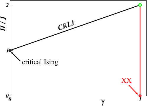
Figure 1: Phase diagram of a single anisotropic $XY$-chain in a magnetic field in the $\gamma-H$ plane: the vertical red line at $\gamma=1$ corresponds to the $XX$-line, while the black line corresponds to the CKL1 $H/J=1+\gamma$. The CKL1 intersects the $XX$-line at its endpoints, $(H,\gamma)=(2J,1)$, highlighted as a red filled black full dot. The opposite endpoint of CKL1, $(H,\gamma)=(J,0)$, corresponds to a critical quantum Ising chain in a transverse magnetic field and is denoted by a black filled point. The merging of the two lines is also denoted by a green dot.

3.1 Poor Man’s Renormalization Group

To implement Poor Man’s RG approach to the effective Kondo Hamiltonian at the junction, we begin by making a weak-interaction assumption for $H_{\Delta}$, which allows us to perturbatively account for the boundary interaction by referring to the disconnected chain limit as a reference paradigm. To determine the energy eigenmodes and eigenfunctions in this limit, we consider the explicit diagonalization of a single anisotropic $XY$-chain with open boundary conditions (OBC), which we discuss in detail in B. The starting point is the partition function, which we present as ${\cal Z}={\cal Z}_{0}\langle{\bf T}_{\tau}[\exp{(-S_{\Delta})}]\rangle$, with ${\bf T}_{\tau}$ being the imaginary time-ordered operator and the boundary action at imaginary times given by

$$S_{\Delta}=2\sum_{\lambda=1}^{3}\>\int_{0}^{\beta}\>d\tau\>[J_{1}\Sigma_{1}^{\lambda}(\tau)+J_{2}\Upsilon_{1}^{\lambda}(\tau)]{\cal R}^{\lambda}(\tau)\;\;\;\;.$$ (11)

In Eq.(11) we have set $J_{1}=J_{\Delta},J_{2}=\gamma^{\prime}J_{\Delta}$. Moreover $\beta=(k_{B}T)^{-1}$, $k_{B}$ being the Boltzmann constant (set to $1$ in the following for the sake of simplicity) and $T$ the temperature. In the standard RG approach to the Kondo problem, as the Kondo Hamiltonian represents a marginal boundary operator, typically one expands $\exp{(-S_{\Delta})}$ up to second-order in $S_{\Delta}$ and then performs the appropriate two-fermion contractions, resulting in a cutoff-dependent correction to $J_{1},J_{2}$. This implies a logarithmic rise of the running couplings, due to the infrared divergences in the fermion propagators. To accomplish this point, it is useful to rewrite $S_{\Delta}$ in terms of the real $\mu$-fermions we introduce in A, which are related to the $c_{j,\lambda}$ fermions by means of the relation $c_{j,\lambda}=\frac{1}{2}[\mu_{2j-1,\lambda}+i\mu_{2j,\lambda}]$. The result is

$$S_{\Delta} = -\sum_{\lambda,\lambda^{\prime}}\sum_{j,j^{\prime}=1,2}\frac{J_{j,j^{\prime}}}{2}\>\int_{0}^{\beta}\>d\tau\>\sigma^{\lambda}(\tau)\sigma^{\lambda^{\prime}}(\tau)\mu_{j,\lambda}(\tau)\mu_{j^{\prime},\lambda^{\prime}}(\tau)$$ (12)

$$= \sum_{\lambda}\sum_{j,j^{\prime}=1,2}2J_{j,j^{\prime}}\frac{1}{\beta}\>\sum_{\Omega}{\cal R}^{\lambda}(\Omega){\cal M}^{\lambda}_{j,j^{\prime}}(-\Omega)\>\>\>\>.$$

In Eq.(12) we have set $J_{1,1}=J_{1}$, $J_{2,2}=J_{2}$ and, in order to account for all the possible corrections arising from the second-order contractions, we introduced two additional effective couplings $J_{1,2},J_{2,1}$, which are set to $0$ in the bare action. Moreover, on the second line we moved to the Matsubara-Fourier space and introduced the operator ${\cal M}_{j,j^{\prime}}(\tau)$ given by

$$\vec{\cal M}_{j,j^{\prime}}(\tau)=-\frac{i}{2}\left[\begin{array}[]{c}\mu_{j,2}(\tau)\mu_{j,3}(\tau)\\ \mu_{j,3}(\tau)\mu_{j,1}(\tau)\\ \mu_{j,1}(\tau)\mu_{j,2}(\tau)\end{array}\right]\>\>\>\>.$$ (13)

Incidentally, it is worth stressing here that the real fermions $\mu_{j,\lambda}$, with $j=1,2$, physically reside at the same site (the first one) of the spin chains. Thus, the action $S_{\Delta}$ in Eq.(12) is a pure boundary one, as it only involves fermions at the first site of the chains. In order, now, to trade our perturbative derivation of the corrections to the coupling strengths for renormalization group equations in a ”canonical” form we first of all assume that the temperature is low enough to trade the discrete sums over Matsubara frequencies for integrals. As per the standard derivation of Poor Man’s scaling equations, to regularize the integrals at high frequencies we introduce an ultraviolet (i.e., high-energy) cutoff $D$. This implies rewriting Eq.(12) as

$$S_{\Delta}\approx\sum_{\lambda}\sum_{j,j^{\prime}=1,2}2J_{j,j^{\prime}}\int_{-D}^{D}\>\frac{d\Omega}{2\pi}\>{\cal R}^{\lambda}(\Omega){\cal M}^{\lambda}_{j,j^{\prime}}(-\Omega)\>\>\>\>.$$ (14)

In order to derive the RG equations for the running couplings, let us now rescale the cutoff from $D$ to $D/\kappa$, with $0<\kappa-1\ll 1$. In order to do this, we split the integral over $[-D,D]$ into an integral over $[-D/\kappa,D/\kappa]$ plus integrals over values of $\Omega$ within $[D/\kappa,D]$ and within $[-D,-D/\kappa]$. In this latter integrals, we eventually integrate over the field operators. Therefore, from Eq.(14) we obtain, apart for a correction to the total free energy, which we do not consider here, as we are mainly interested in the running coupling renormalization

$$S_{\Delta}\to\int_{-\frac{D}{\kappa}}^{\frac{D}{\kappa}}\>\frac{d\Omega}{2\pi}\>{\cal R}^{\lambda}(\Omega){\cal M}^{\lambda}_{j,j^{\prime}}(-\Omega)=\frac{1}{\kappa}\int_{-D}^{D}\>\frac{d\Omega}{2\pi}\>{\cal R}^{\lambda}\left(\frac{\Omega}{\kappa}\right){\cal M}^{\lambda}_{j,j^{\prime}}\left(-\frac{\Omega}{\kappa}\right)\;\;\;\;,$$ (15)

which, in view of the fact that $S_{\Delta}$ corresponds to a marginal boundary interaction and, therefore, must be scale invariant, implies

$${\cal R}^{\lambda}\left(\frac{\Omega}{\kappa}\right){\cal M}^{\lambda}_{j,j^{\prime}}\left(-\frac{\Omega}{\kappa}\right)=\kappa{\cal R}^{\lambda}(\Omega){\cal M}^{\lambda}_{j,j^{\prime}}(-\Omega)\>\>\>\>.$$ (16)

Let us, now, look for second-order corrections to the running couplings. To this order, we obtain a further correction $\delta S_{\Delta}^{(2)}$ to the first-order action by summing over intermediate states with energies within $[D/\kappa,D]$ and within $[-D,-D/\kappa]$. Due to the reality of the $\mu_{j,\lambda}$’s, differently from what happens with the usual Kondo problem, to second order in $S_{\Delta}$, there is only one diagram effectively contributing to the corresponding renormalization of each running coupling, which we draw in Fig.2. Once the appropriate contractions have been done, the corresponding correction to $S_{\Delta}$ is given by

Figure 2: Diagrammatic representation of the first- and second-order (in $J_{\Delta}$) scattering processes arising from the perturbative expansion in a power series of $S_{\Delta}$: a) First-order scattering vertex between $\mu$- and $\sigma$-fermions; b) Second-order loop process renormalizing the scattering amplitude to order $J_{\Delta}^{2}$. Notice that there is only one loop diagram effectively renormalizing the coupling to second order in $J_{\Delta}$, at variance with what happens in the ”ordinary” Kondo problem [2].

$$\delta S_{\Delta}^{(2)}=\sum_{\lambda}\sum_{j,j^{\prime}=1,2}2J_{j,j}J_{j^{\prime},j^{\prime}}\int_{-D}^{D}\>\frac{d\Omega}{2\pi}\>{\cal R}^{\lambda}(\Omega){\cal M}^{\lambda}_{j,j^{\prime}}(-\Omega)[\Gamma^{j,j^{\prime}}(D;\eta)+\Gamma^{j,j^{\prime}}(-D;\eta)]D(1-\kappa^{-1})\>\>\>\>.$$ (17)

with $\Gamma^{j,j^{\prime}}(\Omega)$ being the Fourier-Matsubara transform of $\Gamma^{j,j^{\prime}}(\tau)=G_{j,j}(\tau)g(\tau)$, the single-fermion Green’s functions $G_{j,j}(\tau)$ being listed in Eqs.(95), and $g(\tau)={\rm sgn}(\tau)$ being the $\sigma$-fermion Green’s function $g(\tau)=\langle{\bf T}_{\tau}[\sigma(\tau)\sigma(0)]\rangle$, that is

$$\Gamma^{1,1}(\Omega) = \frac{1}{\beta}\>\sum_{\omega}g(\Omega-\omega)G^{1,1}(\omega)$$

$$\Gamma^{2,2}(\Omega) = \frac{1}{\beta}\>\sum_{\omega}g(\Omega-\omega)G^{2,2}(\omega)$$

$$\Gamma^{1,2}(\Omega) = \frac{1}{\beta}\>\sum_{\omega}g(\Omega-\omega)G^{1,2}(\omega_{m})$$

$$\Gamma^{2,1}(\Omega) = \frac{1}{\beta}\>\sum_{\omega}g(\Omega-\omega)G^{2,1}(\omega)\>\>\>\>.$$ (18)

When trading the sums over Matsubara frequencies for integrals, one has to introduce an infrared cutoff $\eta\sim\pi T$ to cut the divergency in $g(\Omega-\omega)=2/(i\Omega-i\omega)$ arising as $\omega\to\Omega$. Clearly, $\eta$ is related to the difference between fermionic and bosonic Matsubara frequencies, that is, $\eta\sim\pi T$. Accordingly, in Eq.(17) we evidenced the explicit dependence of $\Gamma^{j,j^{\prime}}$ on both $\Omega$ and on the cutoff $\eta$. In fact, rigorously performing the sum over the fermionic Matsubara frequencies already allows us to explicitly introduce the cutoff $\eta$, at the price of retaining a parametric dependence of $\Gamma^{j,j^{\prime}}$ on $T$. We therefore obtain

$$\Gamma^{1,1}(\Omega;\eta=\pi T) = -2\sum_{\epsilon>0}\left[\frac{{\cal A}^{2}(\epsilon)\epsilon}{\epsilon^{2}+\Omega^{2}}\right]\tanh\left(\frac{\beta\epsilon}{2}\right)$$

$$\Gamma^{2,2}(\Omega;\eta=\pi T) = =-2\sum_{\epsilon>0}\left[\frac{{\cal B}^{2}(\epsilon)\epsilon}{\epsilon^{2}+\Omega^{2}}\right]\tanh\left(\frac{\beta\epsilon}{2}\right)$$

$$\Gamma^{1,2}(\Omega;\eta=\pi T) = 2i\sum_{\epsilon>0}\left[\frac{{\cal A}(\epsilon){\cal B}(\epsilon)\Omega}{\epsilon^{2}+\Omega^{2}}\right]\tanh\left(\frac{\beta\epsilon}{2}\right)$$

$$\Gamma^{2,1}(\Omega;\eta=\pi T) = -2i\sum_{\epsilon>0}\left[\frac{{\cal A}(\epsilon){\cal B}(\epsilon)\Omega}{\epsilon^{2}+\Omega^{2}}\right]\tanh\left(\frac{\beta\epsilon}{2}\right)\>\>\>\>.$$ (19)

The explicit formula for the functions ${\cal A}(\epsilon),{\cal B}(\epsilon)$ on the CKL1 is given in Eqs.(94), while the one along the $XX$-line is given in Eq.(96). At the special points corresponding to a $Y$-junction of critical quantum Ising chains, they take the simplified expression in Eq.(101). Now, since $\Gamma^{2,1}(\Omega;\eta)$ is an odd function of $\Omega$, we get no renormalization for the $J_{1,2},J_{2,1}$ that, therefore, get stuck at their bare values $J_{1,2}=J_{2,1}=0$. At variance, $J_{1,1},J_{2,2}$ get renormalized to

$$J_{1,1} \to J_{\Delta}-2J_{\Delta}^{2}\Gamma^{1,1}(D;\eta)D(1-\kappa^{-1})=J_{1,1}-2J_{1,1}^{2}\Gamma^{1,1}(D;\eta)D(1-\kappa^{-1})$$

$$J_{2,2} \to J_{\Delta}\gamma^{\prime}-2J_{\Delta}^{2}(\gamma^{\prime})^{2}\Gamma^{2,2}(D;\eta)D(1-\kappa^{-1})=J_{2,2}-2J_{2,2}^{2}\Gamma^{2,2}(D;\eta)D(1-\kappa^{-1})\>\>\>\>.$$ (20)

As a result, to leading order in $1-\kappa^{-1}$, we obtain that the variations of the running couplings as a function of $1-\kappa^{-1}$ is given by

$$\delta J_{1,1} = -J_{1,1}^{2}\Gamma^{1,1}(D;\eta)D(1-\kappa^{-1})$$

$$\delta J_{2,2} = -J_{2,2}^{2}\Gamma^{2,2}(D;\eta)D(1-\kappa^{-1})\;\;\;\;.\>\>\>\>.$$ (21)

From the perturbative result in Eqs.(21) one works out the renormalization group equations for the running couplings $J_{j,j}(D)$, with $D$ being the running scaling parameter. Specifically, one obtains

$$\frac{dJ_{1,1}(D)}{d\ln\left(\frac{D_{0}}{D}\right)} = J_{1,1}^{2}(D)\rho_{1,1}(D;\eta)$$

$$\frac{dJ_{2,2}(D)}{d\ln\left(\frac{D_{0}}{D}\right)} = J_{2,2}^{2}(T)\rho_{2,2}(D;\eta)\>\>\>\>.$$ (22)

In Eqs.(22) we have denoted with $D_{0}$ a high-energy cutoff which we take equal to the upper-energy band edge, namely, $D_{0}=2J(1+\gamma)$, and have expressed the RG equations in terms of the functions $\rho_{j,j^{\prime}}(D;\eta)$ whose explicit form will be provided below in the various cases of interest. It is important to evidence, here, that, despite their non-orthodox form, the RG equations in Eqs.(22) are expected to rigorously describe the scaling of the running couplings as a function of $D$. Indeed, we first of all notice the presence, at the right-hand side of Eqs.(22), of the functions $\rho_{j,j}$. This is typical of Kondo problems [2] in the case in which one has an energy-dependent local density of states, (such as in the case of Kondo effect with superconducting leads [43, 44, 45]). Moreover, we also note the apparent additional dependence of the functions $\rho_{j,j}(D;\eta)$ on $T$. In fact, this dependence enters just parametrically, through the infrared cutoff $\eta$ and, at least at the initial cutoff rescaling step, is completely unrelated to the one on the scaling parameter $D$. At high enough temperature (that is, when $T$ works as the ”natural” infrared cutoff of the theory), on rescaling the cutoff, the scaling trajectory is traversed from the initial scale $D_{0}$ and the initial coupling strengths $J_{j,j}(D_{0})$, to an effective bandwidth $D_{*}\sim 2\pi T$ and to effective running coupling strengths $J_{j,j}(T)$, which become effectively temperature-dependent, whose dependence on $T$ can be deduced from integrating Eqs.(22) from $D=D_{0}$ to $D=2\pi T$ [2]. In fact, up to subleading contributions in $D^{-1}$, this is formally equivalent to solving the set of differential equations obtained by regarding the temperature $T$ as a running parameter, which is given by

$$\frac{dJ_{1,1}(T)}{d\ln\left(\frac{D_{0}}{T}\right)} = J_{1,1}^{2}(T)\rho_{1,1}(D=2\pi T;\eta=\pi T)$$

$$\frac{dJ_{2,2}(T)}{d\ln\left(\frac{D_{0}}{T}\right)} = J_{2,2}^{2}(T)\rho_{2,2}(D=2\pi T;\eta=\pi T)\>\>\>\>.$$ (23)

Eqs.(23) provide the reference differential system which we use in the following to determine the RG parameter flow in the various regimes of interest. Once the running couplings $J_{j,j}(T)$ have been determined, we resort to the effective ”renormalized” boundary action by simply substituting, in Eq.(12), $J_{j,j^{\prime}}$ with $J_{j,j^{\prime}}(T)$, that is

$$S_{\Delta}\to\sum_{\lambda}\sum_{j,j^{\prime}=1,2}2J_{j,j^{\prime}}(T)\int_{-D}^{D}\>\frac{d\Omega}{2\pi}\>{\cal R}^{\lambda}(\Omega){\cal M}^{\lambda}_{j,j^{\prime}}(-\Omega)\;\;\;\;,$$ (24)

with $J_{j,j}(T)$ obtained by integrating Eqs.(23). In order to recast the formulas for $J_{j,j}(T)$ in a formula useful for our further discussions, we follow Ref.[52] in introducing the ”critical couplings” $J_{j,j}^{c}$ defined as

$$J_{j,j}^{c}\equiv\left\{\int_{0}^{D_{0}}\>\rho_{j,j}(x)\;\frac{dx}{x}\right\}^{-1}\>\>\>\>,$$ (25)

in terms of which we obtain

$$J_{j,j}(T)=\frac{J_{j,j}^{(0)}J_{j,j}^{c}}{J_{j,j}^{c}-J_{j,j}^{(0)}+J_{j,j}^{c}J_{j,j}^{(0)}\int_{0}^{T}\>\rho_{j,j}(x)\;\frac{dx}{x}}\>\>\>\>,$$ (26)

with $J_{j,j}^{(0)}=J_{j,j}(D_{0})$. Within Poor Man’s RG approach, the onset of the Kondo regime corresponds to the existence of a scale $T_{K}$ at which the denominator of Eqs.(26) is equal to $0$. Clearly, for channel-$j$ such a condition can only met provided $J_{j,j}^{(0)}>J_{j,j}^{c}$. Notice that $j=1,2$, so, with ”channel-$1$” we refer to the first pair of Konddo channels and with ”channel-$2$” to the other pair.

By integrating Eqs.(23), we now perform the perturbative RG analysis of the phase diagram of our $Y$-junction along the gapless lines in Fig.1. In particular, the cornerstones of our discussion will be the endpoint of the CKL1 at $\gamma=0$, where one recovers the junctions of three critical quantum Ising chains, discussed in [18, 14, 36], and the endpoint at $\gamma=1$, shared with the $XX$-line. At the former point, we solve the RG equations and provide the corresponding estimate for the Kondo temperature $T_{K}(\gamma=0)$, which is consistent with the formula presented in [18], once one resorts to consistent measure units for the temperature. At the latter point, we show that the 4CK Hamiltonian at a junction of three $XX$-quantum spin chains which, when $-2J\leq H\leq 2J$, provides an extension of the specific system at $H=0$ discussed in [17], turns into an effective 2CK Hamiltonian, due to a combined effect of the breaking of the rotational spin symmetry in the bulk Hamiltonian $H_{XY}$, as well as in the boundary Kondo Hamiltonian $H_{\Delta}$. When moving along the CKL1, that is, when letting $\gamma$ continuously evolve from $\gamma=1$ to $\gamma=0$, we show that the system keeps hosting two-channel Kondo effect. Therefore, from the qualitative point of view, any $\gamma<1$ is equivalent to $\gamma=0$, that is, at low temperatures/energies, the system flows towards the two-channel Kondo fixed point (2CKFP) described in [50]. In fact, while the explicit form of the leading boundary operator arising at the 2CKFP changes depending on whether $\gamma=0$, or $0<\gamma<1$, there are no qualitative changes in the behavior of the system. Remarkably, this happens notwithstanding that, on increasing $\gamma$ towards $\gamma=1$, at a critical value of $\gamma$, $\gamma_{c}^{(2)}$, both couplings $J_{1}(T)$ and $J_{2}(T)$ become relevant, as $J_{1}(T)$ crosses over towards the strong coupling regime before $J_{2}(T)$, due to the combined effect of having $\gamma<1$ and $J_{1,1}(D_{0})>J_{2,2}(D_{0})$.

3.2 Onset of the Kondo regime along the critical Kitaev line

We now discuss the perturbative RG approach to Kondo effect along the CKL1. In fact, as it can be readily inferred from Eq.(2), reversing the sign of the bulk applied magnetic field $H$ is equivalent to performing the canonical uniform transformation

$$\left(\begin{array}[]{c}S_{j,\lambda}^{x}\\ S_{j,\lambda}^{y}\\ S_{j,\lambda}^{z}\end{array}\right)\longrightarrow\left(\begin{array}[]{c}S_{j,\lambda}^{x}\\ -S_{j,\lambda}^{y}\\ -S_{j,\lambda}^{z}\end{array}\right)\;\;\;\;,$$ (27)

that is, a uniform rotation by $\pi$ along the $x$-axis in spin space. Therefore, our analysis can be readily extended to the symmetric CKL2 which we do not discuss in detail here. To recover the RG flow of the running couplings $J_{1,1}(T),J_{2,2}(T)$, we need the explicit formulas for $\rho_{1,1}(T)=\rho_{1,1}(D=2\pi T;\eta=\pi T)$ and for $\rho_{2,2}(T)=\rho_{2,2}(D=2\pi T;\eta=\pi T)$. In the large-$\ell$ limit, these are given by

$$\rho_{1,1}(T) = \frac{4}{\pi TJ(1+\gamma)}\int_{\frac{1}{2\pi}}^{\frac{J(1+\gamma)}{\pi T}}\>du\>\frac{u(1-\delta)\Sigma\left(\frac{2\pi Tu}{J(1+\gamma)}\right)}{(1+\delta)(1+u^{2})^{2}}\>e^{\beta_{q}}\tanh{(\pi u)}$$

$$\rho_{2,2}(T) = \frac{4}{\pi TJ(1+\gamma)}\int_{\frac{1}{2\pi}}^{\frac{J(1+\gamma)}{\pi T}}\>du\>\frac{u(1+\delta)\Sigma\left(\frac{2\pi Tu}{J(1+\gamma)}\right)}{(1-\delta)(1+u^{2})^{2}}\>e^{-\beta_{q}}\tanh{(\pi u)}\>\>\>\>,$$ (28)

with $\delta=\frac{1-\gamma}{1+\gamma}$, the integration variable $u=\epsilon/(2\pi T)$, the function $\Sigma(x)$ given by

$$\Sigma(x)=\frac{\sqrt{2}}{1-\delta^{2}}\Biggl{\{}\sqrt{\delta^{4}+(1-\delta^{2})x^{2}}-\delta^{2}-\frac{1-\delta^{2}}{2}x^{2}\Biggr{\}}^{\frac{1}{2}}\>\>\>\>,$$ (29)

and $e^{\pm\beta_{q}}=\cosh(\beta_{q})\pm\sinh(\beta_{q})$ are defined from Eqs.(88) of B. Along the CKL1 the critical couplings only depend on $\gamma$, that is, $J_{j,j}^{c}=J_{j,j}^{c}(\gamma)$.

Using the explicit formulas for $\rho_{j,j}(T)$ in Eqs.(28), from Eq.(25) we numerically evaluate $J_{j,j}^{c}(\gamma)/[J(1+\gamma)]$ for $0\leq\gamma\leq 1$. The results are reported in Fig.3. As it can be seen from the figure, $J_{1,1}^{c}(\gamma)/[J(1+\gamma)]$ keeps constantly different from zero and increases as $\gamma$ moves from $\gamma=0$ to $\gamma=1$, implying that, the closer one gets to the isotropic $XX$-line, the harder is to develop Kondo effect in channel-$1$. On the other hand, $J_{2,2}^{c}(\gamma)/[J(1+\gamma)]$ increases as $\gamma$ increases towards 1, till the curves for $J_{1,1}^{c}(\gamma)/[J(1+\gamma)]$ and for $J_{2,2}(\gamma)^{c}/[J(1+\gamma)]$ merge into each other, as $\gamma=1$. Thus, at variance with what happens in channel-$1$ (i.e., in the first pair of Kondo channels), the closer $\gamma$ is to 1, the easier for the system is to develop Kondo effect in channel-$2$ (i.e., in the other). At the intersection between the CKL1 and the $XX$-line the two critical couplings are equal to each other and 4CK effect is recovered. To highlight what happens between the two endpoints of the CKL1, it is useful to think about it starting from the intersection point with the $XX$-line. This point belongs to the critical line hosting an effective 4CK Hamiltonian. 4CK effect can be broken down to 2CK effect by either breaking spin rotational invariance about the $z$-axis in the bulk, or in the boundary interaction Hamiltonian (or in both of them). When moving to $\gamma<1$ one is acting on the bulk spectrum: the breaking of the bulk spin rotational invariance about the $z$-axis suddenly implies a switch from 4CK- to 2CK-effect, which persists and gets more and more robust, as long as one moves from $\gamma=1$ towards the Ising limit $\gamma=0$. The analogous breakdown of the spin rotational invariance about the $z$-axis in $H_{\Delta}$ due to $\gamma^{\prime}<1$ just enforces the effect of the bulk spin anisotropy, but is not an essential ingredient, at least along the CKL1, where the system is effectively described in terms of an effective 2CK Hamiltonian, even at $\gamma^{\prime}=1$.

To complement the result emerging from the analysis of the critical couplings as functions of $\gamma$, we numerically compute the Kondo temperatures $T_{K;(1,1)}(\gamma),T_{K;(2,2)}(\gamma)$, respectively associated to $J_{1,1}(T),J_{2,2}(T)$, as a function of $\gamma$ at given bare couplings $J_{1,1}^{(0)}/D_{0}=0.7$ and $J_{2,2}^{(0)}/D_{0}=\gamma J_{1,1}^{(0)}/D_{0}$ (which corresponds to the ”natural choice” $\gamma^{\prime}=\gamma$). To do so, we start from Eqs.(26) for $J_{1,1}(T),J_{2,2}(T)$ and identify $T_{K(1,1)}(\gamma)$ [$T_{K(2,2)}(\gamma)$] as the value of $T$ at which the denominator of the formula for $J_{1,1}(T)$ [$J_{2,2}(T)$] becomes equal to $0$. The results are reported in Fig.4. First of all, consistently with the behavior of the curves for $J_{1,1}^{c}(\gamma)/[J(1+\gamma)]$ and for $J_{2,2}^{c}(\gamma)/[J(1+\gamma)]$, we find that $T_{K;(1,1)}(\gamma)>T_{K;(2,2)}(\gamma)$ $\forall 0\leq\gamma<1$. In particular, we find $T_{K(1,1)}(\gamma=0)\approx 0.016$, which is consistent with the result predicted using the formula for the Kondo temperature of a junction of three critical quantum Ising chains provided in [18] pertinently rewritten in our units, that is, $T_{K,{\rm Ising}}\sim\frac{J}{2\pi}\exp\left(-\frac{2\pi J}{2J_{1,1}^{(0)}}\right)$. In general, moving from $\gamma=0$ to $\gamma=1$, we find a remarkable lowering of $T_{K(1,1)}(\gamma)$. This can be roughly understood by recalling that the development of the Kondo effect is mainly due to infrared divergences close to the Fermi level of itinerant fermions. We may, therefore, estimate $T_{K(1,1)}(\gamma)$ by pertinently approximating $\rho_{1,1}(T)$ in Eqs.(28) (that is, by setting $\tanh\left(\frac{z}{2u}\right)\approx 1$ (which amounts to state that only the low-temperature regime matters in determining $T_{K}$), which leads to the equation

$$\frac{1-\delta}{1+\delta}\>\frac{2J}{J_{1,1}^{(0)}}=\frac{16\pi}{(1+\gamma)}\>\int_{t_{K}}^{\frac{1}{\pi}}\>du\>\int_{0}^{2}\>dz\>\frac{uz\sin{k}}{(z^{2}+4\pi^{2}u^{2})^{2}}\>e^{\beta_{q}}\>\>\>\>\>,$$ (30)

with $t_{K}=T_{K(1,1)}/(2J)$. Eq.(30) can be further simplified by noting that only the integration region around $z=0$ is actually ”sensible” to infrared divergences. Therefore, we approximate $\sin(k)$ and $e^{\beta_{q}}$ to leading order in $z$ and, at the same time, we introduce a cutoff $\lambda(\gamma)$ to cut the integral over high values of $z$. As a result, we are able to further approximate Eq.(30) as

$$\frac{1-\delta}{1+\delta}\>\frac{2J}{J_{1,1}^{(0)}}\approx\frac{2}{\pi(1+\gamma)}\>\frac{4\delta^{2}}{1-\delta^{2}}\int_{0}^{\lambda(\gamma)}\>dz\>\left(\frac{z}{z^{2}+4\pi^{2}t_{K}^{2}}-\frac{z}{z^{2}+4}\right)\>\>\>\>.$$ (31)

The cutoff in Eq.(31) is chosen so that $2\pi T_{K(1,1)}(\gamma)/(2J)\ll\lambda(\gamma)\ll 2$. On integrating Eq.(31) one therefore obtains

$$T_{K(1,1)}(\gamma)\approx\frac{2J(1+\gamma)\lambda^{2}(\gamma)}{4\pi}\>\exp\left[-\frac{\pi 2J(1+\delta)^{2}}{8\delta J_{1,1}^{(0)}}\right]\>\>\>\>.$$ (32)

As $\delta\to 1$ ($\gamma\to 0$), Eq.(32) gives back the result for $T_{K,{\rm Ising}}$, provided the cutoff is chosen so that $\lim_{\gamma\to 0}\lambda(\gamma)=1$. In general, comparing Eq.(32) with the plot in Fig.4, one may infer that $\lambda(\gamma)$ must be a smooth function of $\gamma$ around $\gamma=0$ while, for $\gamma\to 1$, Eq.(32) apparently fails to describe the numerically derived curve for $T_{K(1,1)}(\gamma)$. This is due to the fact that in this limit the density of states close to the Fermi level is no more constant, but decreases as $|\epsilon|^{\frac{1}{2}}$, which makes less effective the effect of low-energy excitations close to the Fermi level and, therefore, less reliable the approximation we performed. Finally, we note that, consistently with the result drawn in Fig.3, $T_{K(2,2)}(\gamma)=0$ for $0\leq\gamma\leq\gamma_{c}\approx 0.92$, which means that no Kondo effect develops in channel-$2$ for $\gamma\leq\gamma_{c}$.

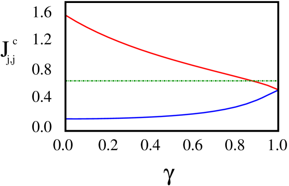
Figure 3: Normalized critical couplings $J_{1,1}^{c}/[J(1+\gamma)]$ (blue curve) and $J_{2,2}^{c}/[J(1+\gamma)]$ (red curve) as functions of $\gamma$. The dashed red line is a guide to the eye, corresponding to $J_{1,1}^{(0)}/D_{0}=0.7$, which is the value we use to compute the Kondo temperature as a function of $\gamma$ for both channels.

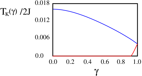
Figure 4: Kondo temperature $T_{K(1,1)}(\gamma)/J$ (blue curve) and $T_{K(2,2)}(\gamma)/J$ (red curve), computed for $J_{1,1}^{(0)}/D_{0}=0.7$ and $J_{2,2}^{(0)}=\gamma J_{1,1}^{(0)}$ (see text). Consistently with the plot in Fig.3, one sees that $T_{K(2,2)}(\gamma)=0$ for $0\leq\gamma<\gamma_{c}$, with $\gamma_{c}\approx 0.92$. Also, one sees that $T_{K(1,1)}(\gamma)$ keeps constantly lower than $T_{K(2,2)}(\gamma)$, implying a $T=0$ fixed point qualitatively equal to the ”pure” two-channel Kondo picture of the junction of three Ising chains [18]. When $\gamma\to 1$ ($XX$-limit), the curves for $T_{K(1,1)}(\gamma)$ and $T_{K(2,2)}(\gamma)$ collapse onto each other, consistently with the four-channel Kondo picture of the junction of three $XX$-chains [17].

We numerically checked that, changing the values of $J_{1,1}^{(0)},J_{2,2}^{(0)}$ and alledging $\gamma^{\prime}\neq\gamma$, provides results only quantitatively different, but qualitatively similar, to what we draw in Fig.4. Therefore, we conclude that such a behavior of the Kondo temperatures associated to the two channels is quite a typical feature of the CKL1.

As a next step, we now infer what is the $T=0$ fixed point of the system along the CKL1 by implementing the approach of [50], which we review and adapt to our specific case in A. To begin with, consistently with the perturbative RG analysis, we assume that, at a given $\gamma$, on lowering $T$ all the way down to $T_{K(1,1)}(\gamma)$, the system reaches a ”putative” fixed point, where the running coupling $J_{1,1}(T)$ has crossed over towards the strongly-coupled regime, while $J_{2,2}(T)$ keeps finite (and perturbative). Consistently with the analysis of [50], this is a two-channel Kondo fixed point (2CKFP), with an additional perturbation proportional to the ”residual” coupling $J_{2,2}(T_{K(1,1)})$. Therefore, we recover the two degenerate singlet ground states $|\Sigma\rangle_{1},|\Sigma\rangle_{2}$ defined in Eqs.(66) and, as a leading perturbation at the 2CKFP, we obtain the operator $H_{\rm Sc}^{(2)}$ in Eq.(71) which, written in terms of the $c$-fermions, is given by

$$H_{\rm Sc}^{(2)} = i\frac{JJ_{2}}{2J_{1}}{\bf V}^{y}\{(1+\gamma)\prod_{\lambda=1,2,3}[(-i)(c_{1,\lambda}-c_{1,\lambda}^{\dagger})]+i\gamma[(c_{1,1}-c_{1,1}^{\dagger})(c_{2,2}-c_{2,2}^{\dagger})(c_{1,3}-c_{1,3}^{\dagger})$$ (33)

$$+ (c_{1,1}-c_{1,1}^{\dagger})(c_{1,2}-c_{1,2}^{\dagger})(c_{2,3}-c_{2,3}^{\dagger})+(c_{2,1}-c_{2,1}^{\dagger})(c_{1,2}-c_{1,2}^{\dagger})(c_{1,3}-c_{1,3}^{\dagger})]\}\;\;\;\;,$$

with the operator ${\bf V}^{y}$ directly connecting the two groundstates: ${\bf V}^{y}|\Sigma\rangle_{1(2)}=-(+)i|\Sigma\rangle_{2(1)}$ (see A for details). $H_{\rm Sc}^{(2)}$ is a trilinear functional of fermionic operators. Therefore, it has scaling dimension $d_{\rm Sc}^{(2)}=\frac{3}{2}>1$ and, accordingly, it is irrelevant at low energies/temperatures. A systematic Schrieffer-Wolff (SW) procedure, implemented by pertinently developing the formalism we use in A to construct $H_{\rm Sc}^{(2)}$, shows that any other allowed boundary operator at 2CKFP-fixed point is less relevant than $H_{\rm Sc}^{(2)}$. As a result, we conclude that, since there are no relevant boundary operators arising at the 2CKFP, this is the actual infrared stable fixed point of the system, along the whole CKL1. Therefore, along this line the system is qualitatively equivalent to the 2CK-system emerging at a junction of three quantum Ising chains [18, 14, 36, 37], with the only difference that, in this latter case, $H_{\rm Sc}^{(2)}$ is replaced with the third-order operator in Eq.(73). At variance, as we are going to discuss next, along the $XX$-line the $Y$-junction may either host 4CK-, or 2CK-physics, depending in this case only on the specific value of the boundary parameter $\gamma^{\prime}$.

3.3 Kondo effect along the $XX$-line

The mapping of a $Y$-junction of three XX quantum spin chains ($\gamma=1$) at zero applied magnetic field ($H=0$) onto an effective Kondo Hamiltonian has been discussed in [17] by assuming symmetric couplings $J_{1,1}^{(0)}=J_{2,2}^{(0)}$ (that is, $\gamma^{\prime}=1$). As a result, it has been found that such a system hosts a remarkable spin-chain realization of a 4CK-Hamiltonian. Here, we first of all show how the results of Ref.[17] readily extend to the case $H\neq 0,\gamma^{\prime}=1$, thus concluding that the whole $XX$-line, parametrized by $-2J\leq H\leq 2J$, can be regarded as a ”critical” 4CK-line, as long as $\gamma^{\prime}=1$. Therefore, we argue how a breakdown of the boundary coupling symmetry, that is, $\gamma^{\prime}\neq 1$, corresponds to a relevant perturbation that lets the system flow towards a 2CKFP. As a result, we conclude that the lack of rotational symmetry along the $z$-axis in spin space makes the system flow towards a 2CKFP, even if it is ”concentrated” just at the boundary interaction Hamiltonian $H_{\Delta}$.

To extend the discussion of the previous section to the $XX$-line, we note that, at a generic nonzero value of $H$, by direct calculation one obtains

$$\rho_{1,1}(T)=\rho_{2,2}(T)=\frac{16\pi}{J}\>\int_{-2J}^{2J}\>d\epsilon\>\>\frac{T^{2}(\epsilon-H)\sqrt{1-\left(\frac{\epsilon}{2J}\right)^{2}}}{(4\pi^{2}T^{2}+\epsilon^{2})^{2}}\>\tanh\left(\frac{\epsilon-H}{2T}\right)\>\>\>\>.$$ (34)

Using the definition in Eq.(25), we now evaluate the critical couplings $J_{1,1}^{c}(h)=J_{2,2}^{c}(h)$ as a function of $h=H/(2J)$. As a result, we obtain

$$\frac{2J}{J_{1,1}^{c}}=\frac{2J}{J_{2,2}^{c}}=16\pi\>\int_{0}^{\frac{1}{\pi}}\>dx\>\int_{-1}^{1}\>dz\>\frac{x(z-h)\sqrt{1-u^{2}}}{[(z-h)^{2}+(2\pi x)^{2}]^{2}}\>\tanh\left(\frac{z-h}{2x}\right)\>\>\>\>,$$ (35)

with $u=\epsilon/(2J),x=T/(2J)$ (note that, due to the bulk spin rotational symmetry, that is, to the condition $\gamma=1$, the condition $J_{1,1}^{c}(h)=J_{2,2}^{c}(h)$ is automatically recovered). In Fig.5 we plot $J_{1,1}^{c}(h)/(2J)(=J_{2,2}^{c}(h)/(2J)$) as a function of $h$ for $-1\leq h\leq 1$. The plot is even for $h\to-h$, as it can be readily inferred from Eq.(35). As $h\to\pm 1$, $J_{j,j}^{c}(h)$ tends to the same value obtained by sending $\gamma$ to 1 along the CKL1, that is, $J_{j,j}^{c}/(2J)\approx 0.57$. Apparently, Fig.5 shows that, the closer one moves towards the JW-fermion band edges ($h=\pm 1$), the harder is to recover Kondo effect. To double-check this conclusion, we also computed the Kondo temperature $T_{K}(h)$ as a function of $h$ for $-1\leq h\leq 1$, by using the same technique we employed to compute $T_{K}(\gamma)$ along the CKL1. We report the result of our numerical calculation for $T_{K}(h)$ in Fig.6. As an over-all observation, we note that, as stated above, the condition $\gamma=1$ implies that $T_{K}(h)$ is the same for both $J_{1,1}(T)$ and for $J_{2,2}(T)$ (that is the reason why we dropped the channel index from $T_{K}$). Moreover, just as $J_{j,j}^{c}(h)$ is an even function of $h$, such is $T_{K}(h)$, as it appears from Fig.6.

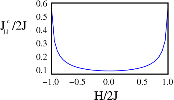
Figure 5: $J_{j,j}^{c}(h)/(2J)$ vs. $h$ along the $XX$-line, parametrized by $-1\leq h\leq 1$. $J_{j,j}(h)$ is an even function of $h$, as it can be inferred from Eq.(35). It is minimum at the point studied in Ref.[17] ($h=0$) and, as $h\to\pm 1$, tends to the same value obtained by sending $\gamma$ to 1 along the CKL, that is, $J_{j,j}^{c}\approx 0.57(2J)$.

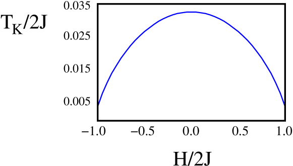
Figure 6: Normalized Kondo temperature $T_{K}/(2J)$ as a function of $h=H/(2J)$ along the $XX$-line. The Kondo temperature is maximum at $h=0$, as expected (see text), while, at the endpoints $h=\pm 1$, we obtain $T_{K}\approx 0.0041(2J)$, which is the same value obtained by moving along the the CKL and towards the endpoint common to the $XX$-line (that is, by sending $\gamma\to 1$ along the CLK).

As for what concerns $T_{K}(h)$, we see that, moving from either endpoint $h=\pm 1$ towards the center of the band ($h=0$), $T_{K}(h)$ increases, till it reaches its maximum exactly at $h=0$. This is, in fact, consistent with the numerical estimate of $J_{j,j}^{c}(h)$ reported in Fig.5, where one sees that $J_{j,j}^{c}(h)$ is maximum at $h=\pm 1$ and decreases on moving from either endpoint towards the center of the band, till it reaches its minimum exactly at $h=0$. Performing approximations analogous to the ones we did in section 3.2, the formula for $T_{K}$ along the $XX$-line can be presented as

$$\frac{2J}{J_{j,j}^{(0)}}\approx\frac{2}{\pi}\>\int_{-1-h}^{1-h}\>dz\>|z|\Biggl{(}\frac{1}{z^{2}+4\pi^{2}t_{K}^{2}}-\frac{1}{z^{2}+4}\Biggr{)}\sqrt{1-(u+h)^{2}}\\ \>\>\>\>,$$

with $t_{K}=T_{K}/(2J)$. For $h=0$ the integral in Eq.(3.3) can be explicitly computed, yielding to the equation

$$\frac{\pi J}{2J_{j,j}^{(0)}}\approx-\ln(\pi t_{K})-\sqrt{5}\>{\rm atanh}\left(\frac{1}{\sqrt{5}}\right)\>\>\>\>,$$ (36)

which, for $J_{j,j}^{(0)}/(2J)=0.7$, yields

$$T_{K}/(2J)\approx 0.035\;\;\;\;,$$ (37)

in good agreement with the numerical data. For a generic value of $h$, assuming again that the relevant contribution to the integral arises from the region nearby $z=0$, one may again introduce an ”ad hoc” cutoff $\lambda(h)$, so to approximate Eq.(3.3) as

$$\frac{2J}{J_{j,j}^{(0)}}\approx\frac{2}{\pi}\>\int_{-\lambda(h)}^{\lambda(h)}\>du\>|u|\Biggl{(}\frac{1}{u^{2}+4\pi^{2}t_{K}^{2}}-\frac{1}{u^{2}+4}\Biggr{)}\sqrt{1-h^{2}}\>\>\>\>,$$ (38)

with, again, $2\pi T_{K}(h)/(2J)\ll\lambda(h)\ll 2$. Eq.(38) is approximatively solved (for small $t_{K}$) by

$$T_{K}(h)\approx\frac{\lambda^{2}(h)J}{2\pi}\>\exp\left[-\frac{\pi 2J}{4J_{j,j}^{(0)}\sqrt{1-h^{2}}}\right]\>\>\>\>,$$ (39)

with $\lambda(h)$ being a smooth function of $h$ around $h=0$, such that $\lambda(0)=\exp\left[-\sqrt{5}\>{\rm atanh}\left(\frac{1}{\sqrt{5}}\right)\right]/\pi$. Again, Eq.(39) fails to predict the finite value of $T_{K}(h)$ as $h\to\pm 1$. The explanation is basically the same as for the limit $\gamma\to 1$, that is, in this limit the density of states close to the Fermi level is no more constant, but decreases as $|\epsilon|^{\frac{1}{2}}$, which makes less effective the effect of low-energy excitations close to the Fermi level and, therefore, less reliable the approximation we performed. The important over-all conclusion is that, moving from the case $h=0$ studied in [17] does not qualitatively change the behavior of the system, but only quantitatively, as only $J_{j,j}^{c}$ and $T_{k}$ are affected. Thus, $h(\in[-1,1])$ appears to parametrize a line of points, all qualitatively equivalent to the one at $h=0$.

While the perturbative RG approach shows the (marginal) relevance of the Kondo-like boundary interaction $H_{\Delta}$, it does not allow for an ultimate characterization of the fixed point toward which the system flows as $T\to 0$. To achieve this task, we have again to resort to a strong-coupling analysis of the boundary interaction. For the sake of the discussion, it is more useful to assume $J_{1,1}^{(0)}\neq J_{2,2}^{(0)}$. In this case, as it is readily inferred from the RG equations for $J_{1,1}(T),J_{2,2}(T)$ in Eqs.(22) and from Eq.(34) for $\rho_{1,1}(T),\rho_{2,2}(T)$, whichever coupling has the larger bare value (say $J_{1,1}$), reaches the strongly coupled regime first, at a Kondo temperature scale $T_{K,1}$. At this scale, the two channels coupled to $J_{1,1}$ develop 2CK effect with the topological spin $\vec{\cal R}$, while the two channels coupled to $J_{2,2}$ keep weakly coupled to $\vec{\cal R}$, with effective coupling $J_{2,2}(T_{K})$. Dubbing such a fixed point 2CKFP1, it is possible to construct the leading boundary perturbation at 2CKFP1 along the procedure outlined in A, exactly as we have done in section 3.2 for the CKL. The result is simply given by Eq.(33) taken in the limit of $\gamma\to 1$, that is

$$H_{\rm Sc;XX}^{(2)} = i\frac{JJ_{2}}{2J_{1}}{\bf V}^{y}\{2\prod_{\lambda=1,2,3}[(-i)(c_{1,\lambda}-c_{1,\lambda}^{\dagger})]+i[(c_{1,1}-c_{1,1}^{\dagger})(c_{2,2}-c_{2,2}^{\dagger})(c_{1,3}-c_{1,3}^{\dagger})$$ (40)

$$+ (c_{1,1}-c_{1,1}^{\dagger})(c_{1,2}-c_{1,2}^{\dagger})(c_{2,3}-c_{2,3}^{\dagger})+(c_{2,1}-c_{2,1}^{\dagger})(c_{1,2}-c_{1,2}^{\dagger})(c_{1,3}-c_{1,3}^{\dagger})]\}\;\;\;\;.$$

Again, the dimension counting yields for $H_{\rm Sc;XX}^{(2)}$ a scaling dimension $d=\frac{3}{2}$, showing the irrelevance of this operator and, accordingly, the stability of the 2CKFP1. Despite the differences in the bulk spectrum, the 2CKFP1 can be ”continuously deformed” to the 2CKFP characterizing the junction along the CKL (at a given $h$ and $\gamma^{\prime}=J_{2,2}(D_{0})/J_{1,1}(D_{0})$, the continuous deformation can be realized, for instance, by first moving to the intersection with the CKL1 (h=1) and, therefore, by further tuning $H$ and $\gamma$ keeping $H=-J(1+\gamma)$, until $\gamma=\gamma^{\prime}$.

At variance, along the symmetric line, parametrized by $h$, corresponding to the symmetric initial condition $J_{1,1}^{(0)}=J_{2,2}^{(0)}$, the above argument does not apply. In this case, based on arguments similar to the ones used by Nozières and Blandin to infer the instability of Nozières Fermi liquid fixed point in the presence of overscreened Kondo effect [53], one expects the system to flow, as $T\to 0$, to a novel fixed point, different from the 2CKFP above. In fact, this can be inferred by directly looking at the boundary Hamiltonian $H_{\Delta}$ in spin coordinates, in the limit $J_{\Delta}/J\to\infty$. To do so, let us generically write $H_{\Delta}$ as

$$H_{\Delta}=-J_{1}\sum_{\lambda=1}^{3}S_{1,\lambda}^{x}S_{1,\lambda+1}^{x}-J_{2}\sum_{\lambda=1}^{3}S_{1,\lambda}^{y}S_{1,\lambda+1}^{y}\equiv H_{\Delta}^{(1)}+H_{\Delta}^{(2)}\>\>\>\>.$$ (41)

As discussed above, an asymmetric initial condition of the form, for instance, $J_{1}^{(0)}>J_{2}^{(0)}$ implies that the running coupling $J_{1}(T)$ reaches the strongly-coupled regime at the Kondo temperature $T_{K}$, at which $J_{2}(T_{K})$ is still finite. At this point, one may attempt to recover the derivation of A by using $H_{\Delta}^{(1)}$ as the unperturbed Hamiltonian and $H^{\prime}$ given by $H^{\prime}=H_{\Delta}^{(2)}+H_{T}$, with

$$H_{T}=-J\sum_{\lambda=1}^{3}\left(S_{1,\lambda}^{x}S_{2,\lambda}^{x}+S_{1,\lambda}^{y}S_{2,\lambda}^{y}\right)$$

as the perturbation. At $J_{1}$ large and positive, the groundstate manifold of $H_{1}$ is twofold degenerate, consisting of the degenerate, fully polarized states $|\Leftarrow\rangle=|\leftarrow,\leftarrow,\leftarrow\rangle$ and $|\Rightarrow\rangle=|\rightarrow,\rightarrow,\rightarrow\rangle$, with $|\leftarrow\rangle$ and $|\rightarrow\rangle$ being the two eigenstates of $S^{x}$. By direct calculation, one finds that all the matrix elements $\langle X|H^{\prime}|X^{\prime}\rangle$, with $|X\rangle,|X^{\prime}\rangle=|\Leftarrow\rangle,|\Rightarrow\rangle$ are zero. As a result, the leading effective boundary Hamiltonian at the strongly-coupled fixed point is recovered to higher order in $H^{\prime}$, by means of a SW procedure that realizes in spin coordinates the analog of what we have done in A using JW fermionic coordinates. As we discuss in A using JW fermions, this leads to an irrelevant operator, which shows the stability of the corresponding strongly coupled fixed point. At variance, in the symmetric case we construct a “putative” fixed point by letting $J_{1}/J=J_{2}/J\to\infty$. This leads to a twofold degenerate groundstate manifold, containing the states $|\Uparrow\rangle,|\Downarrow\rangle$, given by

$$|\Uparrow\rangle = \frac{1}{\sqrt{3}}\{|\uparrow,\uparrow,\downarrow\rangle+|\uparrow,\downarrow,\uparrow\rangle+|\downarrow,\uparrow,\uparrow\rangle\}$$

$$|\Downarrow\rangle = \frac{1}{\sqrt{3}}\{|\downarrow,\downarrow,\uparrow\rangle+|\downarrow,\uparrow,\downarrow\rangle+|\uparrow,\downarrow,\downarrow\rangle\}\>\>\>\>,$$ (42)

with $|\uparrow\rangle,|\downarrow\rangle$ being the eigenstates of $S^{z}$. Clearly, in this case one obtains $H^{\prime}=H_{T}$. By direct calculation one therefore checks that $\langle\Uparrow|H^{\prime}|\Uparrow\rangle=\langle\Downarrow|H^{\prime}|\Downarrow\rangle=0$, while one obtains

$$\langle\Downarrow|H^{\prime}|\Uparrow\rangle = -\frac{2J}{\sqrt{3}}\sum_{\lambda=1}^{3}S_{2,\lambda}^{+}=-\frac{2iJ}{\sqrt{3}}\>\sum_{\lambda=1}^{3}c_{2,\lambda}^{\dagger}\sigma^{\lambda}$$

$$\langle\Uparrow|H^{\prime}|\Downarrow\rangle = -\frac{2J}{\sqrt{3}}\sum_{\lambda=1}^{3}S_{2,\lambda}^{-}=-\frac{2iJ}{\sqrt{3}}\>\sum_{\lambda=1}^{3}c_{2,\lambda}\sigma^{\lambda}\;\;\;\;,$$ (43)

with the right-hand side of Eqs.(43) containing both the spin and the JW-fermion representation of the leading boundary operators at the strongly-coupled fixed point. As a result, in this case, the leading boundary operator at the strongly coupled fixed point can be written as

$$H_{\rm Sc}^{(4)}=-\frac{2iJ}{\sqrt{3}}\{{\bf V}^{-}\sum_{\lambda=1}^{3}c_{2,\lambda}^{\dagger}\sigma^{\lambda}+{\bf V}^{+}\sum_{\lambda=1}^{3}c_{2,\lambda}\sigma^{\lambda}\}\>\>\>\>,$$ (44)

with the operators ${\bf V}^{\pm}$ defined, in analogy to ${\bf V}^{y}$ in Eq.(33), so that ${\bf V}^{+}|\Downarrow\rangle=|\Uparrow\rangle$, ${\bf V}^{-}|\Uparrow\rangle=|\Downarrow\rangle$ and ${\bf V}^{+}|\Uparrow\rangle={\bf V}^{-}|\Downarrow\rangle=0$. As Klein factors and ${\bf V}^{\pm}$ are non dynamical variables, both operators at the right-hand side of Eqs.(44) have scaling dimension $1/2$, which implies that $H_{\rm Sc}^{(4)}$ is a strongly relevant operator. The putative fixed point $J_{1}=J_{2}=\infty$ is therefore not a stable one. Based on arguments analogous to the ones developed in [17], one expects that, in analogy with the overscreened 2CK effect [53], at low temperatures/energies, the system flows towards an intermediate coupling fixed point, which possibly corresponds to the overscreened, spin-$1/2$ four-channel Kondo system [54]. Since any asymmetry between the bare couplings $J_{1,1}(D_{0}),J_{2,2}(D_{0})$ makes the system flow towards a 2CKFP, we then conclude that the symmetric $XX$-line at $J_{1,1}(D_{0})=J_{2,2}(D_{0})$ is a critical 4CK-line marking, at fixed $h$, a quantum phase transition between two 2CK-non-Fermi liquid phases. While it would be extremely interesting to discuss such a quantum phase transition in analogy to what is done, for instance, in [55], where the overscreened 2CK-non-Fermi liquid fixed point is regarded as a quantum phase transition between two perfectly screened 1-channel Kondo Fermi-liquid phases, this goes beyond the scope of this work and, accordingly, we plan to address this issue in a forthcoming publication. In the next section, instead, we discuss a possible tool to detect the onset of Kondo regime by means of an appropriate local magnetization measurement.

4 Kondo-induced crossover in the local transverse magnetization

The onset of Kondo effect is typically associated to a crossover in the effective dependence of running coupling strengths on a dimensionful scale, such as temperature, (inverse) length, etc., as one flows towards the Kondo fixed point: the dependence crosses over from the perturbative RG logarithmic rise, to a specific power-law scale, depending on the particular fixed point describing the system in the zero-temperature, large-scale limit. While in Kondo effect in metals and/or semiconducting devices such a crossover is typically detected by looking at the current transport properties of the system as a function of the running scale, in our $Y$-junction of $XY$-chains there are no free electric charges supporting electrical currents. Therefore, one has to resort to a different tool to monitor the onset of the Kondo regime. Specifically, we propose to look at the local transverse magnetization $m$ at the junction as a function of $T$, as $T$ is lowered all the way down towards $T_{K}$ and then to 0. We define $m$ as

$$m=\frac{1}{3}\>\sum_{\lambda=1}^{3}\langle S_{1,\lambda}^{z}\rangle\>\>\>\>.$$ (45)

We refer to the quantity $m$ defined in Eq.(45) as the local transverse magnetization since the magnetic field $H$ in the Hamiltonian (2) is transverse with respect to the $x-y$ orientation of the spin (the order parameter of the phase transition for the Ising chain being then $\langle S^{x}\rangle$).

As a main motivation for our choice of $m$, we note that it is difficult to implement a local magnetic field acting on the topological spin, which led us to choose a different observable. In terms of the $\mu$-fermions, one can readily compute $m$ as

$$m=\frac{i}{6}\sum_{\lambda=1}^{3}\langle\mu_{1,\lambda}\mu_{2,\lambda}\rangle=\frac{i}{6}\lim_{\eta\to 0^{+}}\>\langle{\bf T}_{\tau}[\mu_{1,\lambda}(\eta)\mu_{2,\lambda}(0)]\rangle\>\>\>\>.$$ (46)

When the chains are disconnected from each other, there is no boundary effects and $m$ takes a finite, ”bare” value $m^{(0)}$, depending on the bulk tuning parameters: $\gamma$ along the CKL1, and $h$ along the $XX$-line. Using the Green’s functions in Eqs.(97), along the CKL1, one obtains

$$m^{(0)}(\gamma)=\frac{1}{2\pi J(1+\gamma)}\int_{0}^{2J(1+\gamma)}\>d\epsilon\>\Sigma\left(\frac{\epsilon}{J(1+\gamma)}\right)\>\>\>\>,$$ (47)

with the function $\Sigma(x)$ defined in Eq.(29). Along the $XX$-line, a similar calculation yields to an integral that can be explicitly calculated, giving the result

$$m^{(0)}(h)=\frac{{\rm arcsin}(h)+h\sqrt{1-h^{2}}}{\pi}\>\>\>\>.$$ (48)

In Fig.7a) we plot $m^{(0)}(\gamma)$ vs. $\gamma$ computed along the CKL using Eq.(47). The plot appears to be consistent with the known results for a single $XY$ model in a transverse field [46, 47, 48], as highlighted in the figure caption. Similarly, in Fig.7b) we plot $m^{(0)}(h)$ vs. $h$ computed along the $XX$-line using Eq.(48). As $h\to 1$, we recover the value $0.5$ for $m^{(0)}(h)$, consistently with the numerical value obtained in the limit $\gamma\to 1$ for $m^{(0)}(\gamma)$ along the CKL. Moreover, $m^{(0)}(h)$ is an odd function of $h$, as expected from the properties of the Hamiltonian under a parity transformation in spin space.

When joining the chains to each other, the onset of the Kondo regime induces an RG flow in the running couplings $J_{j,j}(T)$. Leaving, for the time being, aside the special symmetric case $J_{1,1}^{(0)}=J_{2,2}^{(0)}$ along the $XX$-line, in the previous section we saw that, in all the other cases, the system flows towards a strongly coupled fixed point in either coupling, say $J_{1,1}$, with the other coupling inducing a weak, irrelevant perturbation. Regarding the strongly coupled fixed point in spin coordinates, we see that, in order to minimize the energy, the system lies within a ground state that is either one of the states $|\Rightarrow\rangle,|\Leftarrow\rangle$ introduced above. Since $\langle\Leftarrow|\sum_{\lambda=1}^{3}S_{1,\lambda}^{z}|\Leftarrow\rangle=\langle\Rightarrow|\sum_{\lambda=1}^{3}S_{1,\lambda}^{z}|\Rightarrow\rangle=0$, we find that, as a consequence of the onset of the Kondo regime, $m(T)$ has to flow to zero, as $T$ goes to zero. Moreover, knowing what are the leadingmost boundary operators in the various regimes, allows us to infer the functional dependence of $m(T)$ on $T$ and, eventually, to interpolate the full crossover curve from $m^{(0)}$ all the way down to $m(T\to 0)$.

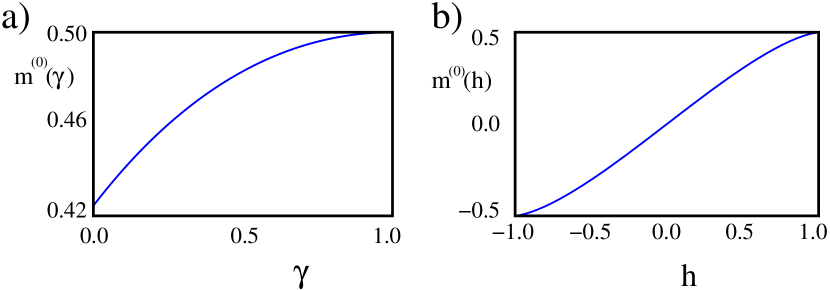
Figure 7: a) Bare magnetization $m^{(0)}(\gamma)$ along the CKL1 as a function of $\gamma$ for $0\leq\gamma\leq 1$. As $\gamma\to 0$, $m^{(0)}(\gamma\to 0)$ gives back the critical magnetization of the ferromagnetic quantum Ising chain, $m^{(0)}(\gamma\to 0)\approx 0.424$, while $m^{(0)}(\gamma\to 1)\to 0.5$; b) $m^{(0)}(h)$ vs. $h$ along the $XX$-line ($-1\leq h\leq 1$). The line corresponds to the paramagnetic phase of the $XX$-model, in which $m^{(0)}(h)$ is an odd function of $h$, and $m^{(0)}(h\to\pm 1)\to\pm 0.5$, as it is appropriate at the paramagnetic-to-ferro(antiferro)magnetic phase transitions.

To investigate the effects of nonzero $J_{1,1}$ and $J_{2,2}$ on $m$ within perturbative RG approach, we first correct $m^{(0)}$ by means of a perturbative calculation in the boundary interaction strengths $J_{1}$ and $J_{2}$. Therefore, employing the standard approximations used in the Kondo problem [2], after computing the correction $\delta m$ to the leading order in $J_{1,1}$ and $J_{2,2}$, we substitute the ”bare” couplings, $J_{1,1}^{(0)},J_{2,2}^{(0)}$, with the running ones, $J_{1,1}(T),J_{2,2}(T)$, as derived in Eq.(26). To second-order in $J_{1,1},J_{2,2}$ one obtains $m=m^{(0)}+\delta m$, with $\delta m$ given by

$$\delta m=-\lim_{\eta\to 0^{+}}\frac{i}{8}\>\sum_{j,j^{\prime}=1,2}J_{j,j}J_{j^{\prime},j^{\prime}}\>\int_{0}^{\beta}\>d\tau_{1}\>d\tau_{2}\>G_{1,j}(\eta-\tau_{1})G_{2,j^{\prime}}(-\tau_{2})G_{j,j^{\prime}}(\tau_{1}-\tau_{2})\>\>\>\>.$$ (49)

From the expressions for the single-fermion Green’s functions in Eqs.(97), in the $T\to 0$-limit, one obtains

$$\delta m = -2J_{1,1}^{2}\>\sum_{\epsilon_{1},\epsilon_{2},\epsilon_{3}>0}{\cal A}^{2}(\epsilon_{1}){\cal A}(\epsilon_{2}){\cal B}(\epsilon_{2}){\cal A}^{2}(\epsilon_{3})\frac{\epsilon_{2}}{(\epsilon_{1}+\epsilon_{2})(\epsilon_{1}+\epsilon_{3})(\epsilon_{2}+\epsilon_{3})}$$ (50)

$$- 2J_{2,2}^{2}\>\sum_{\epsilon_{1},\epsilon_{2},\epsilon_{3}>0}{\cal A}(\epsilon_{1}){\cal B}(\epsilon_{1}){\cal B}^{2}(\epsilon_{2}){\cal B}^{2}(\epsilon_{3})\frac{\epsilon_{1}}{(\epsilon_{1}+\epsilon_{2})(\epsilon_{1}+\epsilon_{3})(\epsilon_{2}+\epsilon_{3})}$$

$$- 2J_{1}J_{2}\sum_{\epsilon_{1},\epsilon_{2},\epsilon_{3}>0}{\cal A}^{2}(\epsilon_{1}){\cal B}^{2}(\epsilon_{2}){\cal A}(\epsilon_{3}){\cal B}(\epsilon_{3})\frac{\epsilon_{3}}{(\epsilon_{1}+\epsilon_{2})(\epsilon_{1}+\epsilon_{3})(\epsilon_{2}+\epsilon_{3})}$$

$$+ 2J_{1,1}J_{2,2}\sum_{\epsilon_{1},\epsilon_{2},\epsilon_{3}>0}{\cal A}(\epsilon_{1}){\cal B}(\epsilon_{1}){\cal A}(\epsilon_{2}){\cal B}(\epsilon_{2}){\cal A}(\epsilon_{3}){\cal B}(\epsilon_{3})\frac{\epsilon_{1}+\epsilon_{2}+\epsilon_{3}}{(\epsilon_{1}+\epsilon_{2})(\epsilon_{1}+\epsilon_{3})(\epsilon_{2}+\epsilon_{3})}\>\>\>\>,$$

with ${\cal A}(\epsilon),{\cal B}(\epsilon)$ defined in Eqs.(94). Regarding, as stated above, $J_{1,1},J_{2,2}$ as running couplings along the CKL1, we obtain

$$\delta m(T;\gamma)=-2J_{1,1}^{2}(T)\>{\cal F}_{1}[\gamma]-2J_{2,2}^{2}(T)\>{\cal F}_{2}[\gamma]-2J_{1,1}(T)J_{2,2}(T)\>\{{\cal F}_{3}[\gamma]-{\cal F}_{4}[\gamma]\}\>\>\>\>,$$ (51)

with

$${\cal F}_{1}[\gamma]=\frac{1}{2}\>\gamma^{2}\>\left(\frac{2}{\pi}\right)^{3}\prod_{j=1}^{3}\left(\int_{0}^{2J(1+\gamma)}\frac{d\epsilon_{j}}{J(1+\gamma)}\>\Sigma\left(\frac{\epsilon_{j}}{J(1+\gamma)}\right)\right)\left[\frac{\epsilon_{2}e^{\beta_{q,1}}e^{\beta_{q,3}}}{(\epsilon_{1}+\epsilon_{2})(\epsilon_{1}+\epsilon_{3})(\epsilon_{2}+\epsilon_{3})}\right]$$

$${\cal F}_{2}[\gamma]=\frac{1}{2}\>\gamma^{-2}\>\left(\frac{2}{\pi}\right)^{3}\prod_{j=1}^{3}\left(\int_{0}^{2J(1+\gamma)}\frac{d\epsilon_{j}}{J(1+\gamma)}\>\Sigma\left(\frac{\epsilon_{j}}{J(1+\gamma)}\right)\right)\left[\frac{\epsilon_{1}e^{-\beta_{q,2}}e^{-\beta_{q,3}}}{(\epsilon_{1}+\epsilon_{2})(\epsilon_{1}+\epsilon_{3})(\epsilon_{2}+\epsilon_{3})}\right]]$$

$${\cal F}_{3}[\gamma]=\frac{1}{2}\>\left(\frac{2}{\pi}\right)^{3}\prod_{j=1}^{3}\left(\int_{0}^{2J(1+\gamma)}\frac{d\epsilon_{j}}{J(1+\gamma)}\>\Sigma\left(\frac{\epsilon_{j}}{J(1+\gamma)}\right)\right)\left[\frac{\epsilon_{3}e^{\beta_{q,1}}e^{-\beta_{q,2}}}{(\epsilon_{1}+\epsilon_{2})(\epsilon_{1}+\epsilon_{3})(\epsilon_{2}+\epsilon_{3})}\right]$$

$${\cal F}_{4}[\gamma]=\frac{1}{2}\>\>\left(\frac{2}{\pi}\right)^{3}\prod_{j=1}^{3}\left(\int_{0}^{2J(1+\gamma)}\frac{d\epsilon_{j}}{J(1+\gamma)}\>\Sigma\left(\frac{\epsilon_{j}}{J(1+\gamma)}\right)\right)\left[\frac{(\epsilon_{1}+\epsilon_{2}+\epsilon_{3})}{(\epsilon_{1}+\epsilon_{2})(\epsilon_{1}+\epsilon_{3})(\epsilon_{2}+\epsilon_{3})}\right]\>\>\>\>.$$ (52)

At variance, along the $XX$-line, we obtain

$$\delta m(T;h)=-2(J_{1,1}(T)-J_{2,2}(T))^{2}\Xi(h)\>\>\>\>,$$ (53)

with

$$\Xi(h)=-\left(\frac{2}{\pi}\right)^{3}\>\int_{-2J-H}^{2J-H}\prod_{i=1}^{3}\left[\frac{d\epsilon_{i}}{2J}\sqrt{1-\left(\frac{\epsilon_{i}+H}{2J}\right)^{2}}\right]\left[\frac{\epsilon_{1}}{(|\epsilon_{1}|+|\epsilon_{2}|)(|\epsilon_{1}|+|\epsilon_{3}|)(|\epsilon_{2}|+|\epsilon_{3})|}\right]\>\>\>\>.$$ (54)

In Fig.8 we draw the four functions ${\cal F}_{j}[\gamma]$, $j=1,2,3,4$, defined in Eqs.(52), as functions of $\gamma$. As expected, ${\cal F}_{1}[\gamma],{\cal F}_{2}[\gamma]$ and ${\cal F}_{3}[\gamma]$ all converge towards the same value ${\cal F}_{*}$ as $\gamma\to 1$, that is, where the CKL meets the $XX$-line, with ${\cal F}_{*}\approx 0.21$. Also as expected, one gets $\lim_{\gamma\to 1}{\cal F}_{4}[\gamma]\approx 0.62=3{\cal F}_{*}$. This is also consistent with the plots of Fig.9, where we display $\Xi(h)$ as a function of $h$ for $-1\leq h\leq 1$. As expected, one obtains $\lim_{h\to 1}\Xi(h)=\Xi_{*}\approx 0.21$, that is, $\Xi_{*}\approx{\cal F}_{*}$, consistent with the ”collapse” of Eq.(51) onto Eq.(53) at the intersection point between the CKL1 and the $XX$-line.

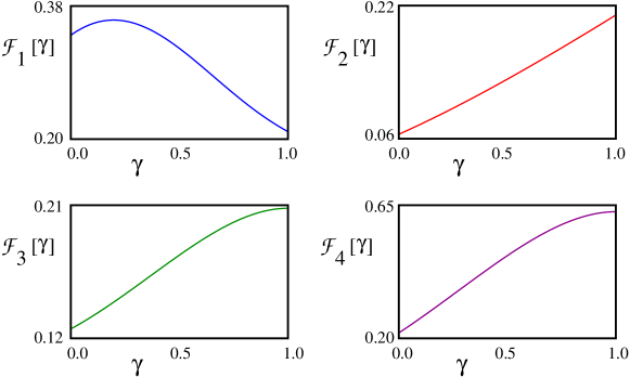
Figure 8: Plot of the four functions ${\cal F}_{j}[\gamma]$ as a function of $\gamma$ for $0\leq\gamma\leq 1$. In detail: a) ${\cal F}_{1}[\gamma]$ for $0\leq\gamma\leq 1$; b) ${\cal F}_{2}[\gamma]$ for $0\leq\gamma\leq 1$; c) ${\cal F}_{3}[\gamma]$ for $0\leq\gamma\leq 1$; d) ${\cal F}_{4}[\gamma]$ for $0\leq\gamma\leq 1$. As it clearly appears from the plots, one obtains $\lim_{\gamma\to 1}{\cal F}_{1}[\gamma]=\lim_{\gamma\to 1}{\cal F}_{2}[\gamma]=\lim_{\gamma\to 1}{\cal F}_{3}[\gamma]\approx 0.21\equiv{\cal F}_{*}$. At variance, $\lim_{\gamma\to 1}{\cal F}_{4}[\gamma]\approx 0.63=3{\cal F}_{*}$.

Figure 9: Plot of $\Xi(h)$ defined in Eq.(54) as a function of $h$ for $-1\leq h\leq 1$. As expected (see text), one obtains $\lim_{h\to 1}\Xi(h)={\cal F}_{*}\approx 0.21$.

Combining Eqs.(51,53) with the numerical solutions of Eqs.(22), we are ultimately able to recover the RG-flow of $m(T)$ along both the CKL1 at fixed $\gamma$ ($m(T,\gamma)$), and the $XX$-line at fixed $h$ ($m(T,h)$). As paradigmatic cases, in Fig.10a) we plot the curve corresponding to $m(T,\gamma=0.005)$ (close to the Ising limit) and in Fig.10b) the curve corresponding to $m(T,\gamma=0.5)$. The interval of values of $T$ we chose ends at $T\sim 2J(1+\gamma)/(2\pi)$, consistent with a full bandwidth of $2J(1+\gamma)$ and with our choice of temperature units, and starts at $T/(J(1+\gamma))\sim 0.055$, where a sensible reduction in $m(T)$ appears as a quite clear evidence of the onset of the Kondo regime. To realize both plots in Fig.10, we have set $J_{1,1}^{(0)}/(J(1+\gamma))=0.5$ and $J_{2,2}^{(0)}=\gamma^{\prime}J_{1,1}^{(0)}$, with $\gamma^{\prime}=\gamma$. A remarkable result is what appears in Fig.11a), where we plot $m(T,\gamma=0.995)$ as a function of $T$. In fact, due to the proximity to the $XX$-line and to the symmetric situation $J_{1,1}^{(0)}=J_{2,2}^{(0)}$, $m(T,\gamma=0.995)$ hardly flows, on lowering $T$, as it can be seen from the plot, where, within the same interval of values of $T$ as in Fig.10a) and in Fig.10b), $m$ varies by less than one part over $10^{4}$, consistent with the fact that, as we discuss in the following, there is no expected flow in $m(T)$ induced by the boundary interaction along the $XX$-line in the case of symmetric coupling. For the sake of completeness, in Fig.11b) we also report the flow of $m(T,h)$ for $h=0.5$ in the case of asymmetric couplings $J_{1,1}^{(0)}=0.5(2J),J_{2,2}^{(0)}=0.35(2J)$. In this case, the running of $m(T,h)$ is again apparent.

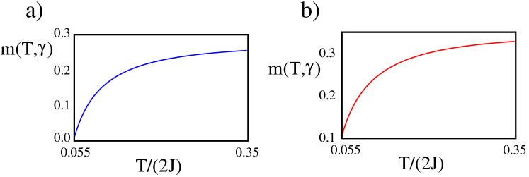
Figure 10: Plot of $m(T,\gamma)$ vs. $T$ in the interval $0.055[(1+\gamma)J]\leq T\leq[(1+\gamma)J]/\pi$ for $J_{1,1}^{(0)}=0.5[J(1+\gamma)]$ and $J^{(0)}_{2,2}=\gamma J_{1,1}^{(0)}$ and for two paradigmatic values of $\gamma$: a) $m(T,\gamma)$ vs. $T$ for $0.055[(1+\gamma)J]\leq T\leq[(1+\gamma)J]/\pi$ and $\gamma=0.005$; b) $m(T,\gamma)$ vs. $T$ for $0.055[(1+\gamma)J]\leq T\leq[(1+\gamma)J]/\pi$ and $\gamma=0.5$. In both cases, on lowering $T$, the reduction in $m(T,\gamma)$ due to the onset of the Kondo regime can be clearly seen.

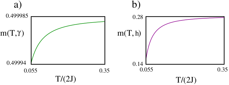
Figure 11: a) Plot of $m(T,\gamma)$ vs. $T$ in the interval $0.055[(1+\gamma)J]\leq T\leq[(1+\gamma)J]/\pi$ for $J_{1,1}^{(0)}=0.5[J(1+\gamma)]$ and $J^{(0)}_{2,2}=\gamma J_{1,1}^{(0)}$ and for $\gamma=0.995$. As expected (see text), there is a rather small percentual change in $m(T,\gamma)$ across the interval of values of $T$ that we consider; b) plot of $m(T,h)$ vs. $T$ in the interval $0.055(2J)\leq T\leq 2J/\pi$ for $h=0.5$ in the case of asymmetric couplings $J_{1}^{(0)}=0.5(2J),J_{2}^{(0)}=0.35(2J)$. In this case, the running of $m(T,h)$ is again apparent.

Before continuing with our discussion, it is now worth focusing onto the symmetric case $J_{1,1}^{(0)}=J_{2,2}^{(0)}$, which we left aside at the beginning, as a special situation. Indeed, in this case, since the symmetry condition among the boundary coupling strengths is preserved along the RG-trajectories, that is, since $J_{1,1}(T)=J_{2,2}(T)$ at any $T$, and because of the commutation relation

$$\left[\frac{1}{3}\sum_{\lambda=1}^{3}S_{1,\lambda}^{z},\sum_{\mu=1}^{3}\left(S_{1,\mu}^{x}S_{1,\mu+1}^{x}+S_{1,\mu}^{y}S_{1,\mu+1}^{y}\right)\right]=0\>\>\>\>,$$ (55)

one obtains that the magnetization is an exactly conserved quantity of the full Hamiltonian $H_{S}=H_{XY}+H_{\Delta}$ and, accordingly, that it is not renormalized by the Kondo interaction. This is definitely consistent with the plot drawn in Fig.11a), where practically no flow of $m(T,\gamma)$ as a function of $T$ appears. Since this is clearly a consequence of the enhanced symmetry of the whole Hamiltonian along the $XX$-line, the absence of flow in $m(T)$ can therefore be related to a recovering of the 4CK-effect along this line in the symmetric case.

Based on the evidence arising from the analytical calculation and on plots such as the ones drawn in Figs.10,11, we propose to look at the local magnetization $m(T)$ as a probe of the onset of the Kondo regime. While in the perturbative regime in $J_{1,1},J_{2,2}$ the decrease in the local magnetization is mainly due to logarithmic corrections to $J_{1,1}(T),J_{2,2}(T)$ taking off on lowering $T$, the scaling law with which $m(T,\gamma)$ or $m(T,h)$ flow to zero at the strongly-coupled fixed point can be eventually inferred from the strong-coupling effective theory. To do so, we note that, as we outline in A, at the strongly-coupled fixed point, all the operators at site-1 are ”fused” with the topological spin operators and disappear from the effective boundary Hamiltonian $H_{\rm Sc}^{(2)}$. In order to compute $m$ close to the strongly-coupled fixed point we therefore resort to an alternative strategy, that is, we add to the Hamiltonian $H_{XY}+H_{\Delta}$ a ”source term” $H_{B}$ for the local magnetization, given by

$$H_{B}=-\frac{B}{3}\>\sum_{\lambda=1}^{3}S_{1,\lambda}^{z}=-\frac{iB}{6}\>\sum_{\lambda=1}^{3}\mu_{1,\lambda}\mu_{2,\lambda}\>\>\>\>.$$ (56)

We therefore compute the partition function at nonzero $B$, ${\cal Z}[B]$, close to the strongly-coupled fixed point and eventually calculate $m$ as

$$m=\frac{1}{\beta}\>\frac{\partial\ln{\cal Z}[B]}{\partial B}\Biggr{|}_{B=0}\>\>\>\>.$$ (57)

Using Eq.(76) for the residual boundary Hamiltonian at the strongly coupled fixed point, one may compute $\ln{\cal Z}[B]$ to leading order in $H_{\rm Sc;B}^{(2)}$. The leading nonzero contribution comes from processes like the ones sketched in the Feynman diagram we draw in Fig.12, where the vertex $\alpha=\frac{1}{2}\left(\frac{J_{2,2}}{J_{1,1}}\right)[J(1+\gamma)+B]$, the full lines represent the propagation of the $\mu$-fermion and the dashed line corresponds to the propagation of the $V^{y}$-operator. The analytical result is given by

$$\ln{\cal Z}[B]\approx\ln\tilde{\cal Z}_{0}+\frac{1}{8}\left(\frac{J_{2,2}}{J_{1,1}}\right)^{2}[J(1+\gamma)+B]^{2}\>\int_{0}^{\beta}\>d\tau_{1}\>d\tau_{2}\>[G_{2,2}(\tau_{1}-\tau_{2})]^{3}\>{\cal G}_{\bf V}(\tau_{1}-\tau_{2})\>\>\>\>,$$ (58)

with $\tilde{\cal Z}_{0}$ being the partition function for the three disconnected wires with all the terms involving the operators $\mu_{1,\lambda}$ dropped out of the Hamiltonian $H_{XY}$, ${\cal G}_{\bf V}(\tau_{1}-\tau_{2})\equiv\langle{\bf T}_{\tau}{\bf V}^{y}(\tau_{1}){\bf V}^{y}(\tau_{2})\rangle={\rm sgn}(\tau_{1}-\tau_{2})$, and $G_{2,2}(\tau_{1}-\tau_{2})$ given in Eq.(95). Without entering the details, we may readily infer the large-$\tau$ limit of $G_{2,2}(\tau)$ by only retaining leading contributions, as $\epsilon\to 0$, in the argument of the corresponding integral in Eq.(95).

Figure 12: Diagrammatic representation of the leading contribution to the strong coupling partition function from the effective boundary Hamiltonian $H_{\rm Sc;B}^{(2)}$. Specifically, $\alpha=\frac{1}{2}\left(\frac{J_{2,2}}{J_{1,1}}\right)[J(1+\gamma)+B]$, the full lines represent the propagation of the $\mu$-fermion and the dashed line corresponds to the propagation of the $V^{y}$-operator.

Figure 13: Plot of the magnetization as a function of the temperature.

The corresponding result is

$$G_{2,2}(\tau)\approx_{|\tau|\to\infty}\>\frac{2(1+\delta)^{2}}{\pi J(1+\gamma)\delta^{3}}\>\int_{0}^{2J(1+\gamma)}\>d\epsilon\>\left(\frac{\epsilon}{J(1+\gamma)}\right)^{2}e^{-\epsilon|\tau|}{\rm Sgn}(\tau)\>\>\>\>.$$ (59)

Using the result in Eq.(59), one readily finds that the integral at the term $\propto[J(1+\gamma)+B]^{2}$ at the right-hand side of Eq.(58) is independent of $\beta$ (that is, independent of $T$) - see the plots in Fig.14. Therefore, from Eq.(57), we are led to conclude that, as $T\to 0$, $m(T)=BT/T_{K}$, with $B$ being a numerical constant. Knowing that, consistently with the analysis of the phase diagram reported in [50], there are no intermediate-coupling fixed points between the weakly- and the strongly-coupled ones, we may infer that, on lowering $T$, $m(T,u)$ (with $u=\gamma$ along the CKL1 and $u=h$ along the $XX$-line) starts from $m^{(0)}(u)$ and takes a quadratic correction in $J_{1,1},J_{2,2}$, which logarithmically increases with $T$ when approaching $T_{K}$. Eventually, the diagram turns into a linear dependence of $m(T,u)$ on $T/T_{K}$, as $T\to 0$, finally flowing to $0$ at the strongly-coupled fixed point. The corresponding plot is expected to be quite alike to the one reported in Fig.13, an analog of which has been presented in Fig.4 of [31], for a junction of three quantum Ising chains, with the running coupling $D$ to be identified with $T$. Such a scaling diagram is the signature of the onset of the Kondo regime. In particular, the linear dependence of $m(T,u)$ on $T/T_{K}$ for $T/T_{K}\to 0$ is the fingerprint of the 2CK effect [54], which, in this system, takes a peculiar realization, not requiring any fine-tuning of the couplings between itinerant electrons and the magnetic impurity [18]. Thus, we conclude that an experimental measurement of $m(T,u)$ provides an effective tool to monitor the onset of the 2CK effect.

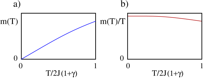
Figure 14: a) Plot of $m(T)$ (arbitrary units) as derived from Eqs.(57,58) across a range of $T$ from 0 to the full bandwidth: as $T\to 0$ (relevant part of the plot) there is an apparent linear dependence on $T$; b) The same plot as in panel a), but multiplied by $\beta(=1/T)$: the flow towards a constant value as $T\to 0$ enforces the linearity of the plot in panel a) as $T\to 0$, but multiplied by $\beta(=1/T)$: the flow towards a constant value as $T\to 0$ enforces the linearity of the plot in panel a) as $T\to 0$.

5 Conclusions

In this paper we have considered a $Y$-junction of anisotropic $XY$ spin chains in a magnetic field, with the chains coupled to each other at a central region determined by the interaction between their initial spins. In general, spin chains offer the possibility of simulating magnetic impurities and to engineer tunable low-energy effective multi-channel Kondo Hamiltonians, in which the symmetry between channels is enforced by RG-flow to low-temperatures/energies [18], differently with what happens with multi-channel Kondo effect in semiconducting devices, such as, for instance, quantum dots, where without fine tuning the parameters, an anisotropy between the two channel emerges, making the coupling to a single channel dominant [56, 57, 58]. In addition, the anisotropic $XY$ model in a magnetic field allows for continuously tuning the bulk parameters keeping the excitation spectrum gapless. Specifically, we showed that, on continuously tuning the bulk parameters of our junction, it is possible to move from a junction of three $XX$-spin chains in an applied magnetic field, to a $Y$-junction of three critical quantum Ising chains, and, in particular, evidenced how this corresponds to an evolution from a four-channel Kondo (4CK) to a two-channel Kondo (2CK) effective Hamiltonian. Moreover, we highlighted that transition from 4CK- to 2CK-effect takes place in a discontinuous way at the merging points between the $XX$-line and the critical Kitaev lines of the $XY$-chains.

The scenario emerging from our analysis implies that, in the case of symmetric boundary couplings ($J_{1}=J_{2}$), the $XX$-line corresponds to a 4CK-critical line, separating two 2CK-phases, towards either one of which the system flows, once the symmetry in the boundary couplings is broken ($J_{1}\neq J_{2}$). Out of the two 2CK-phases separated by the symmetric $XX$-line, one is continuously connected with the 2CK-phase describing the junction along the critical Kitaev lines. Thus, our results point out to the possibility that, at symmetric boundary couplings, the $XX$-line works as a critical line, separating two non-Fermi liquid phases. We believe that this result is important, as it implies the realization, in our junction, of a remarkable quantum phase transition between two non-Fermi liquid phases. In our view, it would be quite interesting to characterize such a quantum phase transition in analogy to what has been done for a quantum dot device in [55], where the 2CK-point has been regarded as the quantum critical point in parameter space, separating two one-channel Kondo Fermi-liquid phases. Nevertheless, a careful characterization of such a quantum phase transition lies beyond the scope of this work, and we plan to leave it aside, for a future investigation.

We finally mention that in the continuous limit both at the $XX$ point and at the critical Ising point the junction boundary term can be exactly treated by Bethe ansatz [36, 37, 38]. This suggests a further interesting development of our research toward studying whether the exact solvability can be extended to the lines of gapless spectrum we discussed in this paper.

Appendix A Spin-isospin representation of the two-channel Kondo Hamiltonian

In this Appendix we discuss a pertinently adapted version of the spin-isospin representation of the spin-$1/2$ two-channel Kondo Hamiltonian introduced in [50], which we use as a guideline to discuss the effective Kondo interaction emerging in our junction. As a starting point, on each chain one trades the $3\ell$ $c_{j,\lambda}$-operators (with $j=1,\ldots,\ell$) for $6\ell$ real fermion operators $\mu_{j,\lambda}$ ($j=1,\ldots,2\ell$), related to each other via

$$c_{j,\lambda}=\frac{1}{2}\left(\mu_{2j-1,\lambda}+i\mu_{2j,\lambda}\right)\>\>\>\>.$$ (60)

The next step is to introduce an additional set of spinful lattice Dirac fermions $\{d_{j,\sigma},d_{j,\sigma}^{\dagger}\}$, with $\sigma=\uparrow,\downarrow$ and $j=1,\ldots,2\ell$. To do so, following [50] we introduce a fourth lattice real fermion $\{\mu_{j,0}\}$ ($j=1,\ldots,2\ell$), which, as we will eventually check, has to decouple from the Kondo boundary interaction and from any relevant physical observable. Therefore, we set

$$d_{j,\uparrow} = \frac{1}{2}\left(\mu_{j,1}+i\mu_{j,2}\right)$$

$$d_{j,\downarrow} = \frac{1}{2}\left(\mu_{j,3}+i\mu_{j,0}\right)\>\>\>\>,$$ (61)

with $j=1,\ldots,2\ell$ [notice that Eqs.(61), though local in the spin index, are non-local in the chain index]. In terms of the $d$-fields one may therefore rewrite $H_{XY}$ as

$$H_{XY} = -\frac{iJ}{2}\>\sum_{j=1}^{2\ell-1}\mu_{j,0}\mu_{j+1,0}-\frac{i\gamma J}{4}\>\sum_{j=1}^{2\ell-3}\delta_{j}\>\mu_{j,0}\left(\mu_{j+1,0}-\mu_{j+3,0}\right)$$ (62)

$$+ iJ\>\sum_{\sigma}\>\sum_{j=1}^{2\ell-1}\>\left(d_{j,\sigma}^{\dagger}d_{j+1,\sigma}-d_{j+1,\sigma}^{\dagger}d_{j,\sigma}\right)$$

$$+ \frac{i\gamma J}{2}\>\sum_{\sigma}\>\sum_{j=1}^{2\ell-1}\>\delta_{j}\,\left(d_{j,\sigma}^{\dagger}d_{j+1,\sigma}-d_{j+1,\sigma}^{\dagger}d_{j,\sigma}\right)$$

$$- \frac{i\gamma J}{2}\>\sum_{\sigma}\>\sum_{j=1}^{2\ell-3}\>\delta_{j}\,\left(d_{j,\sigma}^{\dagger}d_{j+3,\sigma}-d_{j+3,\sigma}^{\dagger}d_{j,\sigma}\right)\>\>\>\>,$$

where $\delta_{j}\equiv 1-(-1)^{j}$. In order to express $H_{\Delta}$ in terms of the $d$-fermions, one defines two commuting lattice vector density operators, a lattice spin density $\vec{\sigma}_{j}$ and an isospin density $\vec{\tau}_{j}$, given by

$$\vec{\sigma}_{j}=\left(\begin{array}[]{c}\sigma_{j}^{1}\\ \sigma_{j}^{2}\\ \sigma_{j}^{3}\end{array}\right)=\frac{1}{2}\left(\begin{array}[]{c}d_{j,\uparrow}^{\dagger}d_{j,\downarrow}+d_{j,\downarrow}^{\dagger}d_{j,\uparrow}\\ -i(d_{j,\uparrow}^{\dagger}d_{j,\downarrow}-d_{j,\downarrow}^{\dagger}d_{j,\uparrow})\\ d_{j,\uparrow}^{\dagger}d_{j,\uparrow}-d_{j,\downarrow}^{\dagger}d_{j,\downarrow}\end{array}\right)\;\;\;,\;\;\vec{\tau}_{j}=\left(\begin{array}[]{c}\tau_{j}^{1}\\ \tau_{j}^{2}\\ \tau_{j}^{3}\end{array}\right)=\frac{1}{2}\left(\begin{array}[]{c}d_{j,\uparrow}^{\dagger}d_{j,\downarrow}^{\dagger}+d_{j,\downarrow}d_{j,\uparrow}\\ -i(d_{j,\uparrow}^{\dagger}d_{j,\downarrow}^{\dagger}-d_{j,\downarrow}d_{j,\uparrow})\\ d_{j,\uparrow}^{\dagger}d_{j,\uparrow}+d_{j,\downarrow}^{\dagger}d_{j,\downarrow}-1\end{array}\right)\;\;\;\;.$$ (63)

In terms of the operators in Eq.(63), one therefore obtains

$$\vec{\Sigma}_{j}=\vec{\sigma}_{2j-1}+\vec{\tau}_{2j-1}\;\;\;,\;\;\vec{\Upsilon}_{j}=\vec{\sigma}_{2j}+\vec{\tau}_{2j}\>\>\>\>,$$ (64)

from which one obtains

$$H_{\Delta}=2J_{\Delta}\left[\left(\vec{\sigma}_{1}+\vec{\tau}_{1}\right)+\gamma^{\prime}\left(\vec{\sigma}_{2}+\vec{\tau}_{2}\right)\right]\cdot\vec{\cal R}\equiv 2\left[J_{1}\left(\vec{\sigma}_{1}+\vec{\tau}_{1}\right)+J_{2}\left(\vec{\sigma}_{2}+\vec{\tau}_{2}\right)\right]\cdot\vec{\cal R}\>\>\>\>.$$ (65)

From Eq.(65) one clearly sees that the ₀-lattice fermions decouple from $H_{\Delta}$, as it should be for the mapping procedure to be consistent. Also, from Eq.(65) it appears that $H_{\Delta}$ describes two pairs of independent spin-$1/2$ lattice density operators, antiferromagnetically coupled to the isolated impurity $\vec{\cal R}$, with coupling strengths $J_{1}=J_{\Delta}$ and $J_{2}=\gamma^{\prime}J_{\Delta}$.

The description in terms of the $d$-spin operators is also effective in working out the ”residual” boundary interaction at the Kondo fixed point, which we used in the main text to discuss the stability of the putative strongly-coupled fixed point in the various regimes. An important preliminary remark is that, on employing the realization of the two-channel spin-$1/2$ Kondo model in terms of spin- and isospin-density operators coupled to a spin-$1/2$ impurity, the isotropic two-channel overscreened Kondo fixed point, which, in the ”standard” realization is known to take place at a finite coupling [53, 54, 61], is pushed towards an effective strongly-coupled fixed point [50]. As discussed in the main text, from the expression of $H_{\Delta}$ we expect that, when the bare coupling $J_{1}$ is $>(<)J_{2}$, the strongly-coupled fixed point of the $Y$-junction corresponds the 2CK-fixed point where the two channels coupled to via $J_{1}$ ($J_{2}$) are strongly-coupled to $\vec{\cal R}$. Assuming for the sake the discussion that $J_{1}$ flows to strong coupling first, in the strongly-coupled limit the groundstate of the system is recovered by minimizing the boundary interaction $\propto J_{1}$. This can be done by noticing that states carrying at site-$j$ spin-$1/2$ associated to the $\vec{\sigma}_{j}$-operators carry spin $0$ associated to the $\vec{\tau}_{j}$-operator, and vice versa. As a result, at strong coupling, the low-energy manifold consists of the spin singlets $|\Sigma\rangle_{1,2}$, defined as

$$|\Sigma\rangle_{1} = \frac{1}{\sqrt{2}}\{d_{1,\uparrow}^{\dagger}|\Downarrow\rangle-d_{1,\downarrow}^{\dagger}|\Uparrow\rangle\}$$

$$|\Sigma\rangle_{2} = \frac{1}{\sqrt{2}}\{d_{1,\uparrow}^{\dagger}d_{1,\downarrow}^{\dagger}|\Downarrow\rangle-|\Uparrow\rangle\}\;\;\;\;.$$ (66)

with $|\Uparrow\rangle,|\Downarrow\rangle$ being the spin $\pm 1/2$ eigenstates of ${\cal R}^{3}$, with $\vec{\cal R}\equiv\left({\cal R}^{1}\>,\>{\cal R}^{2}\>,\>{\cal R}^{3}\right)^{T}$ given by Eq.(9). At large, but finite, coupling $J_{1}$, the system can undergo virtual transitions from either singlet in Eqs.(66) to excited states and back to the singlets. These are induced by the ”residual” boundary Hamiltonian $H^{\prime}$, given by

$$H^{\prime}=iJ\sum_{\sigma}\left(d_{1,\sigma}^{\dagger}O_{\sigma}-O_{\sigma}^{\dagger}d_{1,\sigma}\right)+2J_{2}\vec{\cal R}\cdot\left(\vec{\sigma}_{2}+\vec{\tau}_{2}\right)\equiv H^{{}^{\prime}}_{1}+H_{2}^{{}^{\prime}}\;\;\;\;,$$ (67)

with $O_{\sigma}\equiv\left(1+\gamma\right)d_{2,\sigma}-\gamma d_{4,\sigma}$. The summation over virtual transitions can be performed within a systematic Schrieffer-Wolff procedure, which yields to the effective boundary Hamiltonian $H_{\rm Sc}^{(2)}$ whose matrix elements between the singlets $|\Sigma\rangle_{j}$ and $|\Sigma\rangle_{j^{\prime}}$ are given by

$$[H_{\rm Sc}^{(2)}]_{j,j^{\prime}}\approx-\frac{1}{J_{1}}\>\sum_{X}\>{}_{j}\langle\Sigma|H^{\prime}|X\rangle\langle X|H^{\prime}|\Sigma\rangle_{j^{\prime}}\>\>\>\>,$$ (68)

with the sum over the intermediate states $X$ being carried over the (locally) excited triplet states given by

$$|T_{1}\rangle_{1} = d_{1,\uparrow}^{\dagger}|\Uparrow\rangle\;,\;|T_{0}\rangle_{1}=\frac{1}{\sqrt{2}}\left(d_{1,\uparrow}^{\dagger}|\Downarrow\rangle+d_{1,\downarrow}^{\dagger}|\Uparrow\rangle\right)\;,\;|T_{-1}\rangle_{1}=d_{1,\downarrow}^{\dagger}|\Downarrow\rangle$$

$$|T_{1}\rangle_{2} = d_{1,\uparrow}^{\dagger}d_{1,\downarrow}^{\dagger}|\Uparrow\rangle\;,\;|T_{0}\rangle_{2}=\frac{1}{\sqrt{2}}\left(d_{1,\uparrow}^{\dagger}d_{1,\downarrow}^{\dagger}|\Downarrow\rangle+|\Uparrow\rangle\right)\;,\;|T_{-1}\rangle_{2}=|\Downarrow\rangle\>\>\>\>.$$ (69)

On explicitly computing the sum, one obtains the final result which, once expressed back in terms of the $\mu$-fermions, reads

$$[H_{\rm Sc}^{(2)}]_{1,1} = [H_{\rm Sc}^{(2)}]_{2,2}=-\frac{J_{2}^{2}}{2J_{1}}\left(\frac{3}{2}+2\vec{\sigma}_{2}\cdot\vec{\tau}_{2}\right)-\frac{3J^{2}}{4J_{1}}=-\frac{3J_{2}^{2}}{4J_{1}}-\frac{3J^{2}}{4J_{1}}$$

_1,2 $$= -[H_{\rm Sc}^{(2)}]_{2,1}=\frac{JJ_{2}}{2J_{1}}\left[(1+\gamma)\mu_{2,1}\mu_{2,2}\mu_{2,3}-\gamma\left(\mu_{2,1}\mu_{4,2}\mu_{2,3}+\mu_{2,1}\mu_{2,2}\mu_{4,3}+\mu_{4,1}\mu_{2,2}\mu_{2,3}\right)\right]$$

$$\>\>\>\>.$$ (70)

As it appears from Eqs.(70), up to a constant, we can write the effective strong-coupling Hamiltonian as

$$H_{\rm Sc}^{(2)}=i\frac{JJ_{2}}{2J_{1}}{\bf V}^{y}\left[(1+\gamma)\mu_{2,1}\mu_{2,2}\mu_{2,3}-\gamma\left(\mu_{2,1}\mu_{4,2}\mu_{2,3}+\mu_{2,1}\mu_{2,2}\mu_{4,3}+\mu_{4,1}\mu_{2,2}\mu_{2,3}\right)\right]\;\;\;\;.$$ (71)

In Eq.(71) it is ${\bf V}^{y}\equiv\mu_{1,1}\mu_{1,2}\mu_{1,3}$, with ${\bf V}^{y}$ is the operator exchanging the two singlets:

$${\bf V}^{y}|\Sigma\rangle_{1}=-i|\Sigma\rangle_{2}\;\;\;,\;\;{\bf V}^{y}|\Sigma\rangle_{2}=i|\Sigma\rangle_{1}\>\>\>\>.$$ (72)

An important point to stress is that $H_{\rm Sc}$ in Eq.(71) is second-order in $H^{\prime}$ and, specifically, it is $\propto JJ_{2}$. When $J_{2}=0$ (meaning that $\gamma^{\prime}$ is set to $0$ from the very beginning), $H_{\rm Sc}^{(2)}$ is zero, besides a trivial constant shift of the energies. In this case, as it happens in the analysis of the ”standard” 2CK-problem in [50], the residual boundary interaction at strong coupling is recovered to third-order in $H^{\prime}$. When $J_{2}=0$, extending the SW procedure to third-order in $H^{\prime}$ following, for instance, the approach developed in [62], one obtains the effective Hamiltonian $H_{\rm Sc}^{(3)}$ given by

$$H_{\rm Sc}^{(3)}=i\frac{3J^{3}}{4J_{1}^{2}}{\bf V}^{y}[(1+\gamma)\mu_{2,1}-\gamma\mu_{4,1}][(1+\gamma)\mu_{2,2}-\gamma\mu_{4,2}][(1+\gamma)\mu_{2,3}-\gamma\mu_{4,3}]\;\;\;\;.$$ (73)

The operators in Eqs.(71,73) have been used in the main text when discussing the stability of the strongly-coupled fixed point in the various regions of the system’s parameters. An important conclusion from Eqs.(71,73) is that both $H_{\rm Sc}^{(2)}$ and $H_{\rm Sc}^{(3)}$ correspond to irrelevant operators, as they are both obtained as a product of three fermionic fields, with resulting scaling dimension $d_{\rm Sc}=\frac{3}{2}>1$. Since they are by construction the leading boundary perturbation at the strongly-coupled fixed point, this implies the stability of the two-channel state, consistently with the results of [18].

To conclude this Appendix, we now review how the result in Eq.(71) for $H_{\rm Sc}^{(2)}$ is modified by adding to the total Hamiltonian a source term $H_{B}\equiv-\frac{iB}{6}\>\sum_{\lambda=1}^{3}\mu_{1,\lambda}\mu_{2,\lambda}$ for the local magnetization. To begin with, we rewrite $H_{B}$ in terms of the $d$-fermions as

$$H_{B}=\frac{iB}{6}\left[2\left(d_{2,\uparrow}^{\dagger}d_{1,\uparrow}+d_{2,\uparrow}d_{1,\uparrow}^{\dagger}\right)+\left(d_{2,\downarrow}+d_{2,\downarrow}^{\dagger}\right)\left(d_{1,\downarrow}+d_{1,\downarrow}^{\dagger}\right)\right]\>\>\>\>.$$ (74)

Letting $H_{B}$ act onto the groundstates $|\Sigma\rangle_{1},|\Sigma\rangle_{2}$, one obtains the following nonzero matrix elements at the strongly-coupled fixed point

$$~{}_{2}\langle T,1|H_{B}|\Sigma\rangle_{1} = ~{}_{1}\langle T,1|H_{B}|\Sigma\rangle_{2}=-\frac{iB\sqrt{2}}{6}d_{2,\uparrow}$$

$$~{}_{2}\langle T,-1|H_{B}|\Sigma\rangle_{1} = ~{}_{1}\langle T,-1|H_{B}|\Sigma\rangle_{2}=\frac{iB\sqrt{2}}{6}d_{2,\uparrow}^{\dagger}$$

$$~{}_{2}\langle T,0|H_{B}|\Sigma\rangle_{1} = ~{}_{1}\langle T,0|H_{B}|\Sigma\rangle_{2}=-\frac{iB}{6}(d_{2,\downarrow}+d_{2,\downarrow}^{\dagger})\>\>\>\>,$$ (75)

all the other matrix elements being equal to $0$. Using Eqs.(75) it is now straightforward to repeat the SW procedure to recover the effective boundary Hamiltonian at the strongly-coupled fixed point at nonzero $B$, $H_{\rm Sp;B}^{(2)}$. The final result is

$$H_{\rm Sc;B}^{(2)} = i\frac{JJ_{2}}{2J_{1}}{\bf V}^{y}\{(1+\gamma)\mu_{2,1}\mu_{2,2}\mu_{2,3}-\gamma[\mu_{2,1}\mu_{4,2}\mu_{2,3}+\mu_{2,1}\mu_{2,2}\mu_{4,3}+\mu_{4,1}\mu_{2,2}\mu_{2,3}]\}$$ (76)

$$- \frac{JB}{6J_{1}}\>\{O_{\uparrow}^{\dagger}d_{2,\uparrow}+O_{\uparrow}d_{2,\uparrow}^{\dagger}+(O_{\downarrow}+O_{\downarrow}^{\dagger})\}{\bf V}^{z}+\frac{J_{2}B}{2J_{1}}\>i\mu_{2,1}\mu_{2,2}\mu_{2,3}{\bf V}^{y}\>\>\>\>,$$

with ${\bf V}^{y}$ defined as in Eq.(33) and, by analogy, ${\bf V}^{z}$ defined so that ${\bf V}^{z}|\Sigma\rangle_{1}=|\Sigma\rangle_{1}$, ${\bf V}^{z}|\Sigma\rangle_{2}=-|\Sigma\rangle_{2}$. In the main text, we use the result in Eq.(76) to compute the local magnetization close to the strongly-coupled fixed point.

Appendix B Explicit solution of the Kitaev chain with open boundary conditions

In Section 2 we employ the JW transformation to map a junction of three quantum $XY$-spin chains onto a junction of spinless fermionic Kitaev chains. Due to the presence of the boundary at $j=1$, where the chains interact with each other via the boundary Kondo interaction $H_{\Delta}$, in order to perturbatively account for $H_{\Delta}$ one has to use the disconnected chain limit as reference unperturbed limit. Therefore, one has to explicitly determine the energy eigenmodes and eigenfunctions of a single Kitaev model obeying open boundary conditions (OBC). At variance with the straightforward derivation in the case of periodic boundary conditions [49], as far as we know, only very recently the case of OBC for a lattice chain has been explicitly discussed in detailed way in the literature (see the very recent works [59] for the lattice model and [60] in the continuum limit). For this reason we devote this Appendix to review the procedure of solving the Kitaev Hamiltonian corresponding to a single $XY$-chain with OBC. While we restrict our derivation to the large-$\ell$ limit, we eventually argue that our results are consistent with the ones of [59], taken in the appropriate range of values of the parameters.

By means of the JW-transformation, the Hamiltonian for a single $XY$-chain is mapped onto the fermionic Hamiltonian

$$H_{F}=-\frac{J(1+\gamma)}{2}\>\sum_{j=1}^{\ell-1}\left(c_{j}^{\dagger}c_{j+1}+c_{j+1}^{\dagger}c_{j}\right)+\frac{J(1-\gamma)}{2}\sum_{j=1}^{\ell-1}\left(c_{j}c_{j+1}+c_{j+1}^{\dagger}c_{j}^{\dagger}\right)+H\>\sum_{j=1}^{\ell}c_{j}^{\dagger}c_{j}\>\>\>\>.$$ (77)

$H_{F}$ in Eq.(77) is the Kitaev Hamiltonian as presented in [49] to describe a one-dimensional $p$-wave superconductor, with single-fermion normal hopping amplitude $w=\frac{J(1+\gamma)}{2}$, superconducting gap $\Delta=\frac{J(1-\gamma)}{2}$, and chemical potential $\mu=-H$. A generic energy eigenmode of $H_{F}$, $\Gamma_{E}$, is written as

$$\Gamma_{E}=\sum_{j=1}^{\ell}\left(u^{E}_{j}c_{j}+v^{E}_{j}c_{j}^{\dagger}\right)\>\>\>\>,$$ (78)

with the wavefunctions $u^{E}_{j},v^{E}_{j}$ obeying the Bogoliubov-de Gennes (BdG)-equations for a $p$-wave superconductor, given by

$$Eu^{E}_{j} = -\frac{J(1+\gamma)}{2}\left(u^{E}_{j+1}+u^{E}_{j-1}\right)+Hu^{E}_{j}-\frac{J(1-\gamma)}{2}\left(v^{E}_{j+1}-v^{E}_{j-1}\right)$$

$$Ev^{E}_{j} = \frac{J(1+\gamma)}{2}\left(v^{E}_{j+1}+v^{E}_{j-1}\right)-Hv^{E}_{j}+\frac{J(1-\gamma)}{2}\left(u^{E}_{j+1}-u^{E}_{j-1}\right)\>\>\>\>,$$ (79)

which are solved by functions of the form

$$\left(\begin{array}[]{c}u^{E}_{j}\\ v^{E}_{j}\end{array}\right)\equiv\left(\begin{array}[]{c}u^{E}\\ v^{E}\end{array}\right)e^{ikj}\>\>\>\>,$$ (80)

with

$$Eu^{E} = -\left[J(1+\gamma)\cos{k}-H\right]u^{E}-iJ(1-\gamma)\sin{k}v^{E}$$

$$Ev^{E} = iJ(1-\gamma)\sin{k}u^{E}+\left[J(1+\gamma)\cos{k}-H\right]v^{E}\>\>\>\>.$$ (81)

From Eq.(81), one readily derives the dispersion relation

$$E_{k}=\pm\sqrt{[J(1+\gamma)\cos{k}-H]^{2}+J^{2}(1-\gamma)^{2}\sin^{2}{k}}\>\>\>\>.$$ (82)

Before discussing the boundary conditions in $j=1$ and $j=\ell$, we note that, as it appears from Eq.(82), in general the relation dispersion is gapped, with a minimum energy gap $\Delta_{w}={\rm min}\{\Delta_{1},\Delta_{2}\}$, where $\Delta_{1}=J(1-\gamma)\sqrt{1-\frac{H^{2}}{\gamma J^{2}}}$, with the minimum reached at $\cos{k}=\frac{(1+\gamma)H}{2\gamma J}$, and $\Delta_{2}=|J(1+\gamma)-H|$, with the minimum reached at $\cos{k}=1$. For $\gamma=1$, the dispersion relation in Eq.(82) yields a gapless spectrum as long as $-2J\leq H\leq 2J$. This is the gapless $XX$-line, which, through JW-transformation, maps onto a free-fermion chain with OBC. As stated above, here we focus onto the regime with $H\geq 0$. In this case, for $0\leq\gamma<1$, a gapless line appears for $H=J(1+\gamma)$, with the gap closing at $\cos{k}=1$. This is the critical Kitaev line CKL, marking the transition between the topological and the nontopological phase of the Kitaev Hamiltonian in Eq.(77). The union of this line with the $XX$-line defines the region in parameter space characterized by a gapless JW-fermion spectrum.

To discuss the solutions of the BdG equations along the CKL1, let us assume $H=J(1+\gamma)$ and $0\leq\gamma<1$. Setting $E_{k}=\pm\epsilon_{k}$, Eq.(82) implies

$$\epsilon_{k}=2J\left|\sin\left(\frac{k}{2}\right)\right|\>\sqrt{(1+\gamma)^{2}\sin^{2}\left(\frac{k}{2}\right)+(1-\gamma)^{2}\cos^{2}\left(\frac{k}{2}\right)}\>\>\>\>,$$ (83)

with the gap closing at $k=0$ (mod $2\pi$). To impose the appropriate boundary conditions on the open chain, we note that, for generic values of the system parameters, forcing the wavefunction in Eqs.(78) to solve Eqs.(79), necessarily implies $u^{E}_{j=0}=v^{E}_{j=0}=0$, as well as $u^{E}_{j=\ell}=v^{E}_{j=\ell}=0$. On assuming $k$ to be real, it is easy to check that the only degeneracy in the dispersion relation in Eq.(82) is for $k\to-k$. This degeneracy is however not sufficient to construct solutions satisfying the boundary conditions above, which makes it necessary to consider also solutions with complex values of the momentum, provided they are normalizable. In fact, at a given value of $\epsilon_{k}=\epsilon$, there are two corresponding solutions with real momentum $\pm k$ such that

$$\cos k=\frac{(1+\gamma)^{2}}{4\gamma}-\frac{(1-\gamma)^{2}}{4\gamma}\sqrt{1+\frac{4\gamma\epsilon^{2}}{J^{2}(1-\gamma)^{4}}}\>\>\>\>,$$ (84)

as well as two solutions with purely imaginary momentum $\pm iq$, such that

$$\cosh q=\frac{(1+\gamma)^{2}}{4\gamma}+\frac{(1-\gamma)^{2}}{4\gamma}\sqrt{1+\frac{4\gamma\epsilon^{2}}{J^{2}(1-\gamma)^{4}}}\>\>\>\>.$$ (85)

Positive-energy, real-$k$ solutions are constructed by defining $\alpha_{k}$ so that

$$\cos{\alpha_{k}}=\frac{(1+\gamma)\sin\left(\frac{k}{2}\right)}{\sqrt{(1+\gamma)^{2}\sin^{2}\left(\frac{k}{2}\right)+(1-\gamma)^{2}\cos^{2}\left(\frac{k}{2}\right)}}\;\;\;;\;\;\sin{\alpha_{k}}=\frac{(1-\gamma)\cos\left(\frac{k}{2}\right)}{\sqrt{(1+\gamma)^{2}\sin^{2}\left(\frac{k}{2}\right)+(1-\gamma)^{2}\cos^{2}\left(\frac{k}{2}\right)}}\>\>\>\>.$$ (86)

The two independent propagating solutions with real $k$ are therefore given by

$$\left(\begin{array}[]{c}u_{j}^{E}\\ v^{E}_{j}\end{array}\right)_{\pm k}=\left(\begin{array}[]{c}\cos{\left(\frac{\alpha_{k}}{2}\right)}\\ \pm i\sin{\left(\frac{\alpha_{k}}{2}\right)}\end{array}\right)\>e^{\pm ikj}\>\>\>\>.$$ (87)

At variance, to construct solutions with imaginary momentum, we define $\beta_{q}$ so that

$$\cosh{\beta_{q}}=\frac{(1+\gamma)\left|\sinh\left(\frac{q}{2}\right)\right|}{\sqrt{(1+\gamma)^{2}\sinh^{2}\left(\frac{q}{2}\right)-(1-\gamma)^{2}\cosh^{2}\left(\frac{q}{2}\right)}}\;\;\;,\;\;\sinh(\beta_{q})=\frac{(1-\gamma)\cosh\left(\frac{q}{2}\right)}{\sqrt{(1+\gamma)^{2}\sinh^{2}\left(\frac{q}{2}\right)-(1-\gamma)^{2}\cosh^{2}\left(\frac{q}{2}\right)}}\>\>\>\>.$$ (88)

The corresponding solutions are therefore given by

$$\left(\begin{array}[]{c}u_{j}^{E}\\ v^{E}_{j}\end{array}\right)_{\pm iq}=\left(\begin{array}[]{c}\sinh\left(\frac{\beta_{q}}{2}\right)\\ \pm\cosh\left(\frac{\beta_{q}}{2}\right)\end{array}\right)e^{\mp qj}\>\>\>\>.$$ (89)

In the large-$\ell$ limit, the general form of a normalizable, positive-energy solutions will therefore be given by

$$\left(\begin{array}[]{c}u_{j}^{\epsilon}\\ v^{\epsilon}_{j}\end{array}\right)=\beta\sqrt{\frac{2}{\ell}}\Biggl{\{}\frac{\sinh\left(\frac{\beta_{q}}{2}\right)}{\cos\left(\frac{\alpha_{k}}{2}\right)}\>\left(\begin{array}[]{c}\cos\left(\frac{\alpha_{k}}{2}\right)\cos(kj)\\ -\sin\left(\frac{\alpha_{k}}{2}\right)\sin(kj)\end{array}\right)+\frac{\cosh\left(\frac{\beta_{q}}{2}\right)}{\sin\left(\frac{\alpha_{k}}{2}\right)}\>\left(\begin{array}[]{c}\cos\left(\frac{\alpha_{k}}{2}\right)\sin(kj)\\ \sin\left(\frac{\alpha_{k}}{2}\right)\cos(kj)\end{array}\right)-\left(\begin{array}[]{c}\sinh\left(\frac{\beta_{q}}{2}\right)\\ \cosh\left(\frac{\beta_{q}}{2}\right)\end{array}\right)e^{-qj}\Biggr{\}}\>\>\>\>,$$ (90)

with $k$ and $q$ related to $\epsilon$ as from respectively Eq.(84) and Eq.(85) and

$$\beta=\frac{\sin{\alpha_{k}}}{\sqrt{2\left(\cosh{\beta_{q}}+\cos{\alpha_{k}}\right)}}\>\>\>\>.$$ (91)

Finally, from Eqs.(81), we see that negative-energy solutions with energy $-\epsilon$ can be recovered from the positive-energy ones with energy $\epsilon$ by simply swapping $u_{j}^{E}$ and $v_{j}^{E}$ with each other. (Incidentally, we note that, without resorting to the large-$\ell$ limit, one may derive a secular equations for the allowed values of the momentum/energy by imposing OBC at both boundary on a general linear combination of all four the solutions in Eqs.(87,89). Doing so, one obtains that nontrivial solutions are found, provided the momenta satisfy the secular equation

$$\sin^{2}\left[\left(\frac{k-iq}{2}\right)(\ell+1)\right][-1+\cos(\alpha_{k}+i\beta_{q})]+\sin^{2}\left[\left(\frac{k+iq}{2}\right)(\ell+1)\right][1-\cos(\alpha_{k}-i\beta_{q})]=0\>\>\>\>.$$ (92)

Though we have made the exact comparison to the results of [59] only for specific values of the system parameters, we believe it is safe to assume that Eq.(92) is equivalent to the equations of Appendix B of [59] taken in the specific case $H=J(1+\gamma)$.

The formulas we derived above for the wavefunctions allow us to obtain the explicit expressions for the imaginary time JW-fermion operators at $j=1$, in terms of which we eventually derive the real fermion operators $\mu_{1,\lambda}(\tau),\mu_{2,\lambda}(\tau)$, entering the derivation of the RG scaling equations for the running strengths we performed in section 3. The relevant JW-fermion operators are given by

$$c_{1}(\tau) = \sum_{\epsilon>0}\left[u_{1}^{\epsilon}\left(\Gamma_{\epsilon}+\Gamma_{-\epsilon}^{\dagger}\right)e^{-\epsilon\tau}+v_{1}^{\epsilon}\left(\Gamma_{-\epsilon}+\Gamma_{\epsilon}^{\dagger}\right)e^{\epsilon\tau}\right]$$

$$c_{1}^{\dagger}(\tau) = \sum_{\epsilon>0}\left[u_{1}^{\epsilon}\left(\Gamma_{-\epsilon}+\Gamma_{\epsilon}^{\dagger}\right)e^{\epsilon\tau}+v_{1}^{\epsilon}\left(\Gamma_{\epsilon}+\Gamma_{-\epsilon}^{\dagger}\right)e^{-\epsilon\tau}\right]\>\>\>\>.$$ (93)

As for what concerns the corresponding wavefunctions, from the explicit calculations one sees that, for $H=J(1+\gamma)$ and $\epsilon>0$, one obtains the following identities

$${\cal A}(\epsilon) = u_{1}^{\epsilon}+v_{1}^{\epsilon}=2\beta\sqrt{\frac{2}{\ell}}\frac{\sqrt{\delta^{4}+(1-\delta^{2})\left(\frac{\epsilon}{J(1+\gamma)}\right)^{2}}}{\delta(1+\delta)}e^{\frac{\beta_{q}}{2}}$$

$${\cal B}(\epsilon) = u_{1}^{\epsilon}-v_{1}^{\epsilon}=2\beta\sqrt{\frac{2}{\ell}}\frac{\sqrt{\delta^{4}+(1-\delta^{2})\left(\frac{\epsilon}{J(1+\gamma)}\right)^{2}}}{\delta(1-\delta)}e^{-\frac{\beta_{q}}{2}}\>\>\>\>,$$ (94)

with $\delta=(1-\gamma)/(1+\gamma)$. The solutions with negative energy $-\epsilon$ are simply obtained from the ones in Eqs.(94) by swapping $u_{1}^{\epsilon}$ and $v_{1}^{\epsilon}$ with each other. The key quantities we used in section 3 to derive the RG equations for the running coupling strengths are the imaginary-time-ordered Green’s functions $G_{j,j^{\prime}}(\tau)$ for the real fermions $\mu_{1}(\tau)=c_{1}(\tau)+c_{1}^{\dagger}(\tau)$ and $\mu_{2}(\tau)=-i(c_{1}(\tau)-c_{1}^{\dagger}(\tau))$. In terms of the functions ${\cal A}(\epsilon),{\cal B}(\epsilon)$ in Eqs.(94), one obtains

$$G_{1,1}(\tau) = 2\sum_{\epsilon>0}{\cal A}^{2}(\epsilon)\{[1-f(\epsilon)]{\rm sgn}(\tau)e^{-\epsilon|\tau|}+f(\epsilon){\rm sgn}(\tau)e^{\epsilon|\tau|}\}$$

$$G_{2,2}(\tau) = 2\sum_{\epsilon>0}{\cal B}^{2}(\epsilon)\{[1-f(\epsilon)]{\rm sgn}(\tau)e^{-\epsilon|\tau|}+f(\epsilon){\rm sgn}(\tau)e^{\epsilon|\tau|}\}$$

$$G_{1,2}(\tau) = -G_{2,1}(\tau)=-2i\sum_{\epsilon>0}{\cal A}(\epsilon){\cal B}(\epsilon)\{[1-f(\epsilon)]{\rm sgn}(\tau)e^{-\epsilon|\tau|}-f(\epsilon){\rm sgn}(\tau)e^{\epsilon|\tau|}\}\>\>\>\>,$$ (95)

with $f(\epsilon)$ being the Fermi distribution function. Incidentally, we note that Eqs.(95) describe the real-fermion Green’s functions along all the gapless lines, including the $XX$-lines, provided one uses the appropriate expression for ${\cal A}(\epsilon)$ and ${\cal B}(\epsilon)$ which, along this line, is given by

$${\cal A}(\epsilon)={\cal B}(\epsilon)=\sqrt{\frac{2}{\ell}}\>\sqrt{1-\left[\frac{\epsilon+H}{2J}\right]^{2}}\>\>\>\>,$$ (96)

and sums over energies $\epsilon$ such that $-2J-H\leq\epsilon\leq 2J-H$. Resorting to Fourier space to compute $G_{j,j^{\prime}}(i\omega_{m})=\int_{0}^{\beta}\>d\tau\>e^{i\omega_{m}\tau}\>G_{j,j^{\prime}}(\tau)$, with $\omega_{m}=\frac{2\pi}{\beta}\left(m+\frac{1}{2}\right)$ being the $m$-th fermionic Matsubara frequency, one gets

$$G_{1,1}(i\omega_{m}) = -2\sum_{\epsilon>0}{\cal A}^{2}(\epsilon)\left(\frac{1}{i\omega_{m}-\epsilon}+\frac{1}{i\omega_{m}+\epsilon}\right)$$

$$G_{2,2}(i\omega_{m}) = -2\sum_{\epsilon>0}{\cal B}^{2}(\epsilon)\left(\frac{1}{i\omega_{m}-\epsilon}+\frac{1}{i\omega_{m}+\epsilon}\right)$$

$$G_{1,2}(i\omega_{m}) = -G_{2,1}(i\omega_{m})=-2i\sum_{\epsilon>0}{\cal A}(\epsilon){\cal B}(\epsilon)\left(\frac{1}{i\omega_{m}-\epsilon}-\frac{1}{i\omega_{m}+\epsilon}\right)\>\>\>\>.$$ (97)

In the large-$\ell$ limit, the sum over the momenta in the definition of ${\cal A}(\epsilon),{\cal B}(\epsilon)$ can be traded for an integral, which, along the CKL1, eventually yields

$$G_{1,1}(i\omega_{m}) = \frac{8}{\pi J(1+\gamma)}\>\left(\frac{1-\delta}{1+\delta}\right)\>\int_{0}^{2J(1+\gamma)}\>d\epsilon\>\frac{i\omega_{m}e^{\beta_{q}}\Sigma\left(\frac{\epsilon}{J(1+\gamma)}\right)}{\omega_{m}^{2}+\epsilon^{2}}$$

$$G_{2,2}(i\omega_{m}) = \frac{8}{\pi J(1+\gamma)}\>\left(\frac{1+\delta}{1-\delta}\right)\>\int_{0}^{2J(1+\gamma)}\>d\epsilon\>\frac{i\omega_{m}e^{-\beta_{q}}\Sigma\left(\frac{\epsilon}{J(1+\gamma)}\right)}{\omega_{m}^{2}+\epsilon^{2}}$$

$$G_{1,2}(i\omega_{m}) = -G_{2,1}(i\omega_{m})=\frac{8}{\pi J(1+\gamma)}\>\int_{0}^{2J(1+\gamma)}\>d\epsilon\>\frac{i\epsilon\Sigma\left(\frac{\epsilon}{J(1+\gamma)}\right)}{\omega_{m}^{2}+\epsilon^{2}}\>\>\>\>,$$ (98)

with the function $\Sigma(x)$ defined in Eq.(29). Similarly, along the $XX$-line one obtains

$$G_{1,1}(i\omega_{m}) = G_{2,2}(i\omega_{m})=\frac{4}{\pi J}\>\int_{-2J-H}^{2J-H}\>d\epsilon\;\sqrt{1-\left(\frac{\epsilon+H}{2J}\right)^{2}}\>\left[\frac{i\omega_{m}}{\epsilon^{2}+\omega_{m}^{2}}\right]$$

$$G_{1,2}(i\omega_{m}) = -G_{2,1}(i\omega_{m})=\frac{4}{\pi J}\>\int_{-2J-H}^{2J-H}\>d\epsilon\;\sqrt{1-\left(\frac{\epsilon+H}{2J}\right)^{2}}\>\left[\frac{i\epsilon}{\epsilon_{m}^{2}+\omega^{2}}\right]\>\>\>\>.$$ (99)

Both Eqs.(98) and Eqs.(99) have been used in the main text to implement the perturbative expansion in the Kondo-like Hamiltonian representing the junction.

To conclude this Appendix, we report the simplified solution available in the Ising limit $\gamma=0$. In this case, from Eqs.(79), one may readily show that the boundary condition at the left-hand endpoint of the chain implies $u^{E}_{0}-v^{E}_{0}=0$, which can be readily satisfied by setting

$$\left(\begin{array}[]{c}u_{j}^{E}\\ v_{j}^{E}\end{array}\right)=\sqrt{\frac{2}{\ell}}\>\left(\begin{array}[]{c}\cos\left(\frac{\alpha_{k}}{2}\right)\sin\left(kj-\frac{\alpha_{k}}{2}\right)\\ -\sin\left(\frac{\alpha_{k}}{2}\right)\cos\left(kj-\frac{\alpha_{k}}{2}\right)\end{array}\right)\>\>\>\>.$$ (100)

Eq.(100), together with the observation that now one has $\alpha_{k}=\frac{\pi}{2}-\frac{k}{2}$ and $\epsilon=2J\sin\left(\frac{k}{2}\right)$, implies

$${\cal A}(\epsilon) = \sqrt{\frac{2}{\ell}}\sqrt{1-\left(\frac{\epsilon}{2J}\right)^{2}}\left[4\left(\frac{\epsilon}{2J}\right)^{2}-1\right]$$

$${\cal B}(\epsilon) = 2\sqrt{\frac{2}{\ell}}\left(\frac{\epsilon}{2J}\right)\sqrt{1-\left(\frac{\epsilon}{2J}\right)^{2}}\>\>\>\>.$$ (101)

References

- [1] J. Kondo, Progr. Theor. Phys. 32, 37 (1964)
- [2] A. C Hewson, The Kondo problem to heavy fermions, Cambridge University Press (Cambridge, 1993)
- [3] L. Kouwenhoven and L. Glazman, Phys. World 14, 33 (2001)
- [4] A. P. Alivisatos, Science 271, 933 (1996)
- [5] L. Kouwenhoven and C. M. Marcus, Phys. World 11, 35 (1998)
- [6] I. Affleck and S. Eggert, Phys. Rev. B 46, 10866 (1992)
- [7] A. Furusaki and T. Hikihara, Phys. Rev. B 58, 5529 (1998)
- [8] N. Laflorencie, E. S. Sorensen, and I. Affleck, J. Stat. Mech. P02007 (2008)
- [9] I. Affleck, N. Laflorencie, and E. S. Sorensen, J. Phys. A 42, 504009 (2009)
- [10] A. Bayat, P. Sodano, and S. Bose, Phys. Rev. B 81, 064429 (2010)
- [11] P. Sodano, A. Bayat, and S. Bose, Phys. Rev B 81, 100412 (2010)
- [12] A. Deschner and E. S. Andreas, J. Stat. Mech. P10023 (2011)
- [13] A. Bayat, S. Bose, P. Sodano, and H. Johannesson, Phys. Rev. Lett. 109, 066403 (2012)
- [14] A. M. Tsvelik and W.-G. Yin, Phys. Rev. B 88, 144401 (2013)
- [15] A. Bayat, H. Johannesson, S. Bose, and P. Sodano, Nature Comm. 5, 3784 (2014)
- [16] B. Alkurtass, A. Bayat, I. Affleck, S. Bose, H. Johannesson, P. Sodano, E. S. Sorensen, and K. Le Hur, Phys. Rev. B 93, 081106 (2016)
- [17] N. Crampè and A. Trombettoni, Nucl. Phys. B, 871, 526 (2013)
- [18] A. M. Tsvelik, Phys. Rev. Lett. 110, 147202 (2013)
- [19] A. Komnik and R. Egger, Phys. Rev. Lett. 80, 2881 (1998)
- [20] S. Lal, S. Rao, and D. Sen, Phys. Rev. B 66, 165327 (2002)
- [21] C. Chamon, M. Oshikawa, and I. Affleck, Phys. Rev. Lett. 91, 206403 (2003); J. Stat. Mech. P02008 (2006)
- [22] D. Giuliano and P. Sodano, New J. Phys. 10, 093023 (2008); Nucl. Phys. B 811 (2009) 395
- [23] A. Agarwal, Phys. Rev. B 90, 195403 (2014)
- [24] S. Mardanya and A. Agarwal, Phys. Rev. B 92, 045432 (2015)
- [25] D. Giuliano and A. Nava, Phys. Rev. B 92, 125138 (2015)
-
[26]
S. Yin and B. Béri,
arXiv:1507.08632 - [27] R. Burioni, D. Cassi, M. Rasetti, P. Sodano, and A. Vezzani, J. Phys. B 34, 4697 (2001)
- [28] I. Brunelli, G. Giusiano, F.P. Mancini, P. Sodano, and A. Trombettoni, J. Phys. B 37, S275 (2004)
- [29] A. Tokuno, M. Oshikawa, and E. Demler, Phys. Rev. Lett. 100, 140402 (2008)
- [30] A. Cirillo, M. Mancini, D. Giuliano, and P. Sodano, Nucl. Phys. B 852, 235 (2011)
- [31] D. Giuliano and P, Sodano, Europhys. Lett. 103, 57006 (2013)
- [32] F. Iglói, L. Turban, and B. Berche, J. Phys. A: Math. Gen. 24, L1031 (1991)
- [33] P. Jordan and E. Wigner, Z. Phys. 47, 531 (1928)
- [34] B. Béri, B. and N. R. Cooper, Phys. Rev. Lett. 109, 156803 (2012)
- [35] A. Altland, B. Béri, R. Egger, and A. M. Tsvelik, Phys. Rev. Lett. 113, 076401 (2014)
- [36] A. M. Tsvelik, New J. Phys. 16, 033003 (2014)
- [37] A. Altland, B. Béri, R. Egger, and A. M. Tsvelik, J. Phys. A 47, 265001 (2014)
- [38] F. Buccheri, H. Babujian, V. E. Korepin, P. Sodano, and A. Trombettoni, Nucl. Phys. B 896, 52 (2015).
-
[39]
F. Buccheri, G. D. Bruce, A. Trombettoni,
D. Cassettari, H. Babujian, V. E. Korepin, and P. Sodano,
arXiv:1511.06574 - [40] M. R. Galpin, A. K. Mitchell, J. Temaismithi, D. E. Logan, B. Béri, and N. R. Cooper, Phys. Rev. B 89, 045143 (2014).
- [41] A. A. Abrikosov, L. P. Gorkov, and I. Ye. Dzyaloshinski, Quantum field theoretical methods in statistical physics, Pergamon (Oxford, 1965)
- [42] L. I. Glazman and K. A. Matveev, JETP Lett. 49, 659 (1989)
- [43] G. Campagnano, D. Giuliano, A. Naddeo, and A. Tagliacozzo, Physica C 406, 1 (2004).
- [44] F. Siano and R. Egger, Phys. Rev. Lett. 93, 047002 (2004)
- [45] J. S. Lim and M.-S. Choi, J. Phys.: Condens. Matter 20, 415225 (2008)
- [46] E. Lieb, T. Schultz, and D. Mattis, Ann. Phys. (N. Y.) 16, 407 (1961)
- [47] V. E. Korepin, N. M. Bogoliubov, and A. G. Izergin, Quantum Inverse Scattering Method and Correlation Functions, Cambridge University Press (Cambridge, 1997)
- [48] M. Takahashi, Thermodynamics of One-Dimensional Solvable Models, Cambridge University Press (Cambridge, 1999)
- [49] A. Kitaev, Phys.-Usp. 44, 131 (2001)
- [50] P. Coleman, L. B. Ioffe, and A. M. Tsvelik, Phys. Rev. B 52, 6611 (1995)
- [51] F. Franchini, Notes on Bethe Ansatz techniques, available at http://people.sissa.it/ffranchi/BAClass.html/
- [52] L. Dell’Anna, J. Stat. Mech. P01007 (2010)
- [53] P. Nozières and A. Blandin, J. Phys. (Paris) 41, 193 (1980)
- [54] I. Affleck and A. W. W. Ludwig, Nucl. Phys. B 352, 849 (1991); Phys. Rev. Lett. 67, 161 (1991)
- [55] M. Pustilnik, L. Borda, L. I. Glazman, and J. von Delft, Phys. Rev. B 69, 115316 (2004)
- [56] D. Giuliano, B. Jouault, and A. Tagliacozzo, Europhys. Lett. 58, 401 (2002)
- [57] Y. Oreg and D. Goldhaber-Gordon, Phys. Rev. Lett. 90, 136602 (2003)
- [58] R. M. Potok, I. G. Rau, H. Shtrikman, Y. Oreg, and D. Goldhaber-Gordon, Nature 446, 167 (2007)
-
[59]
M. Fagotti,
arXiv:1601.02011 -
[60]
M. Müller and A. A. Nersesyan,
arXiv:1603.01037 - [61] A. W. W. Ludwig and I. Affleck, Phys. Rev. Lett., 67, 3160 (1991)
- [62] D. Giuliano and A. Tagliacozzo, J. Physics: Condens. Matter 16, 6075 (2004)