Percolation in Finite Matching Lattices

Abstract

We derive an exact, simple relation between the average number of clusters and the wrapping probabilities for two-dimensional percolation. The relation holds for periodic lattices of any size. It generalizes a classical result of Sykes and Essam and it can be used to find exact or very accurate approximations of the critical density. The criterion that follows is related to the criterion Scullard and Jacobsen use to find precise approximate thresholds, and our work provides a new perspective on their approach.

I Introduction

For nearly 60 years, percolation theory has been used to model properties of porous media and other disordered physical systems Stauffer and Aharony (1994); *grimmett:book. Its statement is strikingly simple: for site percolation, every site on a specified lattice is independently colored black with probability $p$, or white with probability $1-p$. The sites of the same color form contiguous clusters whose properties are studied. A central quantity is the average number $N_{L}(p)$ of black clusters in a lattice of linear size $L$. According to a classical result of Sykes and Essam Sykes and Essam (1964), certain two-dimensional lattices form matching pairs such that the cluster numbers $N_{L}$ and $\hat{N}_{L}$ of the pair satisfy a relation

$$\lim_{L\to\infty}L^{-2}[N_{L}(p)-\hat{N}_{L}(1-p)]=\chi(p)\,,$$ (1)

where the matching polynomial $\chi(p)$ is a finite, low-order polynomial. The matching lattice for the square lattice is the square lattice with nearest and next-nearest neighbors, and the corresponding matching polynomial is Sykes and Essam (1964)

$$\chi(p)=\chi_{\Box}(p)=p-2p^{2}+p^{4}\,.$$ (2)

Fully triangulated planar lattices like the triangular lattice or the union-jack lattice are self-matching, i. e., $N_{L}(p)=\hat{N}_{L}(p)$, and they all share the same matching polynomial

$$\chi(p)=\chi_{\Delta}(p)=p-3p^{2}+2p^{3}\,.$$ (3)

The Sykes-Essam relation can be used to derive a relation between the percolation thresholds $p_{c}$ of the lattice and $\hat{p}_{c}$ of the matching lattice. If we make the plausible assumption that the asymptotic cluster density $n(p)=\lim_{L\to\infty}L^{-2}N_{L}(p)$ is analytic for all $p\in[0,1]$ except at $p=p_{c}$ (and similarly for the matching lattice), then (1) implies that $p_{c}=1-\hat{p}_{c}$, because the matching polynomial is analytic and the non-analyticities of $n$ and $\hat{n}$ have to cancel. For self-matching lattices like the triangular lattice or the union-jack lattice, this implies $p_{c}=\frac{1}{2}$. The matching polynomial or “Euler Characteristic” has been studied for many lattices by Neher et al. Neher et al. (2008).

Equation (1) is valid only in the limit of infinitely large lattices. In this contribution we will derive its finite-size generalization. In particular we will show that for $L\times L$ lattice with periodic boundary conditions (a torus)

$$N_{L}(p)-\hat{N}_{L}(1-p)-L^{2}\chi(p)=R_{L}^{x}(p)-\hat{R}_{L}^{x}(1-p)\,,$$ (4)

where $R_{L}^{x}$ is the probability that a cluster wraps around the torus in one or both directions (and similarly for $\hat{R}_{L}^{x}$ for the matching lattice). The right-hand side of (4) for the case of wrapping in both directions has been studied recently by Scullard and Jacobsen under the name “critical polynomial” Scullard and Jacobsen (2012). The root of this critical polynomial is a good approximation for the critical density that converges very quickly to $p_{c}$ as $L$ goes to infinity. Our result (4) shows that the critical polynomial can be expressed in terms of the number of clusters as well as in terms of wrapping probabilities.

II Matching Lattices and Euler’s Gem

Figure 1: A configuration $\mathcal{C}$ of black sites on the $20\times 20$ square lattice and the complementary configuration $\hat{\mathcal{C}}$ of white sites on the matching lattice.

Consider a planar lattice like the square lattice. Let us call this the primary lattice. Its matching lattice is obtained by adding edges to each face of the primary lattice such that the boundary vertices of that face form a clique, namely a fully connected graph. For the square lattice this means that we add the two diagonals to each face: the matching lattice of the square lattice is the square lattice with next-nearest neighbors—see Fig. 1.

Now we randomly color each site either black with probability $p$ or white with probabilty $1-p$. The black sites are connected through the edges of the primary lattice whereas the white sites are connected through the edges of the matching lattice. This construction induces a black subgraph $\mathcal{C}$ of the primary lattice and a white subgraph $\hat{\mathcal{C}}$ of the matching lattice (Fig. 1). Obviously each black component is surrounded by white sites and each white component is surrounded by black sites. The crucial observation is that all white sites that surround a black component are connected in $\hat{\mathcal{C}}$, and, vice versa, all black sites that surround a white component are connected on $\mathcal{C}$. Note that this would not be true if both black and white sites inherited their connectivity from the primary lattice (Fig. 2).

Figure 2: White sites surrounding a black cluster (left) or enclosed by a face of the black cluster (right) need not be connected on the primary lattice. But they are always connected on the matching lattice.

Euler’s law of edges (“Euler’s Gem” according to Richeson (2008)) is a beautiful equation that relates the number of vertices $V$, the number of edges $E$, the number of faces $F$ and the number of components $N$ of a planar graph via

$$N=V-E+F\,,$$ (5)

where we do not count the unbounded region outside the graph as a face.

On a lattice with open boundary conditions, the subgraph $\mathcal{C}$ of black vertices would be planar and we could apply (5) to compute the number of its components. On a lattice with periodic boundary conditions (a torus), we need to take into account that some clusters may wrap around the torus, which modifies Euler’s law of edges.

A cluster can wrap around the torus in different ways. The simplest case is a cluster that wraps around along one direction only. Let us call this scenario single wrapping. There can be multiple single-wrapping clusters on a lattice, but notice that for each single-wrapping black cluster on the primal lattice there is one single-wrapping white cluster on the matching lattice, and vice versa.

A cluster can also wrap around both directions, but there are two topologically different ways to do this—see Fig. 3. A single wrapping cluster can tilt enough to also wrap around the other direction, or spiral around the torus. Note that we still can have more than one spiraling cluster and that again the number of spiraling black clusters equals the number of spiraling white clusters. We refer to spiraling clusters as single wrapping clusters, too.

Figure 3: Two topologically distinct ways in which a cluster can wrap around both axes of a two-dimensional periodic lattice. Spiraling (left) versus cross-wrapping (right).

We say that a cluster is cross-wrapping if it wraps around both directions independently. On a cross-wrapping cluster one can walk around the torus to collect any given pair of winding numbers $(n_{x},n_{y})$ around the directions $x$ and $y$. On a spiraling cluster, $n_{x}$ and $n_{y}$ are linearly dependent. Note that there can be at most one cross-wrapping cluster, and a cross-wrapping black cluster on the primal lattice exists if and only if there is no wrapping white cluster on the matching lattice, and vice versa.

If none of the the black clusters wraps, the black subgraph $\mathcal{C}$ is planar, and Euler’s Gem tells us that the number of black clusters is

$$N_{L}=V-E+F\,,$$ (6)

where $V$, $E$ and $F$ now denote the number of vertices, edges and faces of $\mathcal{C}$.

Now imagine that we add more and more edges to the black cluster until the first single wrapping cluster appears. The first edge that establishes the wrapping neither increases $V$, $F$ nor $N_{L}$, but increases $E$. Hence we need to correct Euler’s equation by subtracting $1$ from the left hand side. The same is true for additional single-wrapping clusters. For $k$ single-wrapping clusters we get

$$N_{L}-k=V-E+F\,.$$ (7)

In order to establish a cross-wrapping cluster, we must expend exactly $2$ closing edges that neither increase $V$, $F$ or $N_{L}$. Hence we have

$$N_{L}-2=V-E+F$$ (8)

if $\mathcal{C}$ contains a cross-wrapping cluster. Combining all three cases provides us with

$$N_{L}-(V-E+F)=\begin{cases}0&\text{no wrapping,}\\ k&\text{single-wrapping,}\\ 2&\text{cross-wrapping.}\end{cases}$$ (9)

Some faces of $\mathcal{C}$ are elementary in the sense that they correspond to faces of the underlying primary lattice. Other faces are larger and enclose some empty vertices of the primary lattice. Let $F_{0}$ denote the number of elementary faces of $\mathcal{C}$. Each non-elementary face then encloses exactly one component of white vertices of $\hat{\mathcal{C}}$, but some clusters of‚ $\hat{\mathcal{C}}$ are not enclosed by a face of $\mathcal{C}$. Again we need to discriminate three cases.

If no black cluster wraps around the torus, then there is exactly one cross-wrapping white cluster in $\hat{\mathcal{C}}$, and this is the only white cluster that is not enclosed by a face of $\mathcal{C}$. Hence we have $F=F_{0}+\hat{N}_{L}-1$ in this case. If there are $k$ single-wrapping black clusters, then there are also $k$ single wrapping white clusters, and these are the only white clusters that are not enclosed by black faces: $F=F_{0}+\hat{N}_{L}-k$. Finally, if $\mathcal{C}$ contains a cross-wrapping cluster, none of the white clusters are wrapping, and the white clusters are all enclosed by black faces except the one that borders the cross-wrapping black cluster. Again we have $F=F_{0}+\hat{N}_{L}-1$. In summary,

$$F=F_{0}+\hat{N}_{L}-\begin{cases}1&\text{no wrapping,}\\ k&\text{single-wrapping,}\\ 1&\text{cross-wrapping.}\end{cases}$$ (10)

Combining this with (9) provides us with

$$N_{L}-\hat{N}_{L}-(V-E+F_{0})=\begin{cases}\phantom{-}1&\text{$\mathcal{C}$ cross-wrapping,}\\ -1&\text{$\hat{\mathcal{C}}$ cross-wrapping,}\\ \phantom{-}0&\text{otherwise.}\end{cases}$$ (11)

We take the average over all configurations to finally get

$$N_{L}(p)-\hat{N}_{L}(1-p)-L^{2}\chi(p)=R^{c}_{L}(p)-\hat{R}^{c}_{L}(1-p)$$ (12)

where $R^{c}_{L}$ ( $\hat{R}^{c}_{L}$) denotes the probability that $\mathcal{C}$ ($\hat{\mathcal{C}}$) contains a cross-wrapping cluster, and

$$\chi(p)=L^{-2}\big{(}\langle V\rangle-\langle E\rangle+\langle F_{0}\rangle\big{)}$$ (13)

is the matching polynomial of Sykes and Essam that appears in (1). In fact, for the square lattice we recover $\chi_{\Box}(p)$ of equation (2),

$$\langle V/L^{2}\rangle =p$$ (14)

$$\langle E/L^{2}\rangle =2p^{2}$$

$$\langle F_{0}/L^{2}\rangle =p^{4}\,.$$

Let us denote the left hand side of (12) the matching function $M_{L}(p)$,

$$M_{L}(p)=N_{L}(p)-\hat{N}_{L}(1-p)-L^{2}\chi(p)\,.$$ (15)

Then the Sykes-Essam relation (1) reads

$$\lim_{L\to\infty}L^{-2}M_{L}(p)=0\,,$$ (16)

and (12) can be considered as the finite-size generalization of the Sykes-Essam relation.

We can write the right-hand side of (12) using wrapping probabilities other than $R_{L}^{c}$. Specifically:

• $R^{e}_{L}$ is the probability of any kind of wrapping cluster. This is indicated by a winding number that is nonzero in either coordinate.

• $R^{h}_{L}$ is the probability of a cluster that wraps horizontally, and may or may not also wrap in the vertical direction. This is indicated by a winding number that is nonzero in the first coordinate.

• $R^{s}_{L}$ is the probability of a spiraling cluster that wraps both horizontally and vertically. This is indicated by a single winding number that is nonzero in both coordinates.

• $R^{b}_{L}$ is the probability of any cluster that wraps both horizontally or vertically, no matter whether spiraling or cross-wrapping.

• $R^{1}_{L}(\eta)$ is the probability of a cluster that wraps horizontally, but not vertically. This is indicated by a winding number that is nonzero in only the first coordinate.

Since $R^{c}_{L}=R^{b}_{L}-R^{s}_{L}$ and $R^{s}_{L}(p)=\hat{R}^{s}_{L}(1-p)$, we can write (12) as

$$M_{L}(p)=R^{b}_{L}(p)-\hat{R}^{b}_{L}(1-p)\,.$$ (17)

We also have

$$R_{L}^{e}=2R_{L}^{h}-R_{L}^{b}=2R_{L}^{1}+R_{L}^{b}\,,$$ (18)

and

$$R_{L}^{1}(p)=\hat{R}^{1}_{L}(1-p)\,,$$ (19)

which imply that we can write (12) as

$$M_{L}(p)=R_{L}^{x}(p)-\hat{R}_{L}^{x}(1-p)\qquad x\in\{c,b,e,h\}$$ (20)

for the “cross-wrapping,” “both,” “either” and “horizontal” conditions. This is the main result of this paper.

The only contribution to the right-hand side of (20) comes from the cross-wrapping probabilities. All other wrapping probabilities cancel each other out. But the other wrapping probabilities that include cross-wrapping events can often be computed more efficiently on a computer. The union-find algorithm Newman and Ziff (2001) for example is fastest for computing $R^{e}_{L}$, while the transfer matrix method is best suited for $R^{h}_{L}$.

In their work, Scullard and Jacobsen Scullard and Jacobsen (2012), considered the condition

$$R_{L}^{c}(p)-R_{L}^{0}(p)=0$$ (21)

to estimate $p_{c}$, where $R^{0}(p)$ means that there is no wrapping cluster. This condition says that the probability of wrapping both ways is equal to the probability of wrapping neither way—a generalization of the “all equals none” condition that gives exact thresholds on self-dual triangular hypergraph arrangements Wu (2006); *chayes:lei:06; *ziff:scullard:06; *wierman:ziff:11; *bollobas:riordan:10. But the probability of no wrapping on the lattice is equal to the probability of cross-wrapping on the dual lattice $R_{L}^{0}(p)=\hat{R}_{L}^{c}(1-p)$, and thus we see that (21) is identical to the right-hand side of (12) being equal to 0. Thus we have obtained a new perspective on Scullard and Jacobsen’s criticality criterion.

For self-matching lattices such as the triangular lattice, the union-jack lattice or any other fully triangulated lattice, we have $R_{L}^{x}(p_{c})=\hat{R}_{L}^{x}(p_{c})$ and $p_{c}=1/2$. Hence the right-hand side of (20) vanishes at $p_{c}$ and we have

$$M_{L}(p_{c})=0\qquad\text{(self-matching)}$$ (22)

for all values of $L$.

III Bond Percolation

So far we have focussed on site percolation, but (20) equally well applies to bond percolation. Instead of a matching lattice, we have the dual lattice, also designated by a hat, with bonds occupied with probability $1-p$. We adopt the view of bond percolation in which every site is “wetted,” so that individual isolated sites count as components of size 1. The Euler formula (5) still applies with single components counting as single vertices. In this case, every face on the primal lattice corresponds to one component on the dual lattice, so that $\langle F\rangle=\hat{N}_{L}(1-p)$ and there is no need to isolate $F_{0}$. Furthermore, we have $\langle V\rangle=L^{2}$. Consequently, $\chi(p)$ becomes simply

$$\chi(p)=1-L^{-2}\langle E\rangle$$ (23)

With this version of $\chi$ and with the dual instead of the matching lattice, (20) holds for bond percolation.

For a square lattice of size $L\times L$, we have $\chi(p)=1-2p$. In this case, the dual lattice is identical to the primal lattice, so $\hat{N}_{L}$ = $N_{L}$ and $\hat{R}_{L}^{x}$ = $R_{L}^{x}$. Thus for this system we have $p_{c}=1/2$ and $M_{L}(p_{c})=0$, similar to the self-matching lattices in site percolation.

For the triangular lattice, the dual is the honeycomb, and $\chi(p)=1-3p$. For this system too, the right-hand side of (20) is identically zero for finite systems at the critical point, because at that point the cross-configuration probabilities for triangular and honeycomb lattices are identical. This follows from the star-triangle transformation, which says that on each triangle or enclosed star the connection probabilities are the same at the critical point. Consequently, all configurations between the triangular vertices for a self-dual arrangement of triangles will occur with equal probability, and in particular, the cross-wrapping probability will be the same. Note that the star-triangle transformation applies to single star/triangles at the critical point and there is no need to take the limit of an infinite system here. Hence we have

$$M_{L}(p_{c})=0\qquad\text{(self-dual),}$$ (24)

where self-dual refers to lattices that are either directly self-dual (such as the square lattice) or indirectly via a star-triangle transformation.

Bond percolation on the triangular lattice is but one example for which $p_{c}$ can be computed exactly using the star-triangle transformation or its generalization, the triangle-triangle transformation Ziff (2006); *scullard:06; *bollobas:riordan. This method works in general for lattices that can be decomposed into a regular triangular array of identical triangular cells, as shown in Fig. 4, where the shaded triangles represent any network with bonds. If $P(A,B,C)$ denotes the probability, that all three vertices of the basic triangle are connected, and $P(\overline{A},\overline{B},\overline{C})$ denotes the probability that none of the three vertices are connected, the equation that determines $p_{c}$ is Ziff (2006)

$$\Delta(p)=P(A,B,C)-P(\overline{A},\overline{B},\overline{C})=0\,.$$ (25)

For the triangular lattice one easily gets

$$\Delta(p)=p^{3}-3p+1\,,$$ (26)

with the well-known root Sykes and Essam (1964)

$$p_{c}=2\sin\pi/18=0.3472963553\ldots\,.$$ (27)

For the martini lattice Scullard (2006), the polynomial reads

$$\Delta(p)=(2p^{2}-1)(p^{4}-3p^{3}+2p^{2}+1)\,,$$ (28)

with root

$$p_{c}=\frac{1}{\sqrt{2}}=0.7071067812\ldots\,.$$ (29)

In general, $\Delta(p)$ is a low order polynomial with integer coefficients that shares its root $p_{c}\in(0,1)$ with $M_{L}(p)$.

Figure 4: Decomposition of a lattice into cells (shaded).

The matching function $M_{L}(p)$ is a polynomial with integer coefficients, too, but of order $O(L^{2})$. If it has an algebraic root, it is divisible by the minimal polynomial of that root. Since (26) is irreducible, we know that for bond percolation on the triangular lattice, $M_{L}(p)$ is divisible by $p^{3}-3p+1$ for all $L$. Similarly, $M_{L}(p)$ is divisible by $2p^{2}-1$ for bond percolation on the martini lattice.

IV Applications

The right-hand side of (20) is strictly confined to the interval $[-1,1]$, which immediately tells us that the difference between the number of clusters and the number of holes (or dual-lattice clusters) scales like $L^{2}\chi(p)$:

$$N_{L}(p)-\hat{N}_{L}(1-p)=L^{2}\chi(p)+O(1)\,.$$ (30)

Since both $R_{L}^{x}(p)$ and $-\hat{R}^{x}_{L}(1-p)$ for $x\in\{c,b,e,h\}$ are monotonically increasing functions of $p$, $M_{L}(p)$ is also monotonically increasing. As can be seen in Fig. 5, $M_{L}(p)$ is a sigmoidal function that converges to a step function as $L\to\infty$:

$$\lim_{L\to\infty}M_{L}(p)=\begin{cases}-1&\text{for $p<p_{c}$,}\\ +1&\text{for $p>p_{c}$.}\end{cases}$$ (31)

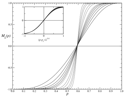
Figure 5: Matching function (15) for the square lattice. Solid curves are from exact enumerations for $L=3\ldots 7$, dashed curves from Monte-Carlo simulations for $L=16,24,32,48$. The inset shows a scaling plot of the data, $M_{L}(p)$ is plotted as a function of $z/b=(p-p_{c})L^{1/\nu}$.

The matching function $M_{L}(p)$ has a unique root $p_{L}^{\star}\in(0,1)$ which converges to the critical density $p_{c}$ as $L\to\infty$. Empirically, the rate of convergence is $p^{\star}_{L}-p_{c}\sim L^{-w}$ with $w\approx 4$ Jacobsen (2014, 2015). This is significantly faster than the convergence of estimators derived from wrapping probabilities in the primary lattice alone, which converge like $p-p_{c}\sim L^{-2.75}$ Newman and Ziff (2001). The convergence of $p_{L}^{\star}$ is so fast that exact solutions of small systems are a better alternative to computing $p_{c}$ than Monte-Carlo simulations of larger systems. This approach has been used in the work of Scullard and Jacobsen Scullard and Jacobsen (2012); Jacobsen (2014, 2015), who computed the ”critical polynomials” (21) exactly using the transfer matrix method. Extrapolating the values of their roots to $L=\infty$ has yielded the most precise estimates of the critical densities for many two-dimensional lattices. Our result (20) provides a new representation of the critical polynomial in terms of cluster numbers or various alternative wrapping probabilities.

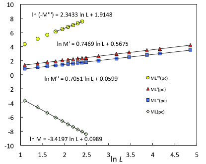
Figure 6: Log-log plot of $-M_{L}^{\prime\prime\prime}(p_{c}),$ $M_{L}^{\prime}(p_{c}),$ $M_{L}^{\prime\prime}(p_{c}),$ $M_{L}(p_{c})$ (top to bottom) vs. $L$, with the linear fit of the data shown for each. For $M_{L}$ we used exact data for $L=3,\ldots,11$ and MC data for $L=12$, for $M_{L}"$ and $M_{L}^{\prime\prime}$ we used MC data up to $L=128$, and for $M_{L}^{\prime\prime\prime}$ we used exact results only. For $M_{L}^{\prime\prime\prime}$ we made a linear fit with only the last six points, $L=6-11.$

The formulation in terms of numbers of clusters on the lattice and dual or matching lattice may be useful for some calculations. We have carried out Monte-Carlo simulations where we simultaneously count the number of clusters on a lattice and its matching lattice for the same configurations, and interestingly find that by doing so the convergence is quicker than simulating clusters on the two lattices independently.

Following the analysis of $N_{L}(p)$ given in Mertens et al. (2016), we can gain some insight into the fast convergence of estimates for $p_{c}$ based upon $M_{L}(p)$. The general scaling for $N_{L}(p)/L^{d}$ for $p$ near $p_{c}$ is given by

$$N_{L}(p)/L^{d}=A_{0}+B_{0}\varepsilon+C_{0}\varepsilon^{2}+D_{0}\varepsilon^{3}+\ldots+L^{-d}f(z)$$ (32)

where $A_{0}$, $B_{0}$, $C_{0}$, $D_{0},\ldots$ are system-dependent constants, $\varepsilon=p-p_{c}$, $f(z)$ is the leading scaling function, and $z=b(p-p_{c})L^{1/\nu}$ where $b$ is a metric factor that is also system dependent. For large $z$, $f(z)$ yields the universal and symmetric singularity $\mathcal{A}|z|^{2-\alpha}$ where $\alpha=-2/3$ in two dimensions.

The scaling function $f(z)$ is universal for systems of the same shape, and is therefore identical to $\hat{f}(z)$ for the matching/dual lattice, as is $b$. Then it follows that

$$M_{L} (p) =N_{L}(p)-\hat{N}_{L}(1-p)-L^{2}\chi(p)$$ (33)

$$= L^{2}\big{[}-\chi(p)+A_{0}+B_{0}\varepsilon+C_{0}\varepsilon^{2}-\ldots$$ (34)

$$- \hat{A}_{0}+\hat{B}_{0}\varepsilon-\hat{C}_{0}\varepsilon^{2}+\ldots\big{]}+f(z)-f(-z)$$ (35)

for $p$ near $p_{c}$. The bracketed term above must go to zero so that $M_{L}(p)$ remains finite as $L\to\infty$, implying that $A_{0}-\hat{A}_{0}=\chi(p_{c})$, $B_{0}+\hat{B}_{0}=\chi^{\prime}(p_{c})$, $C_{0}-\hat{C}_{0}=\chi^{\prime\prime}(p_{c})/2$, etc. Thus we have

$$M_{L}(p)=f(z)-f(-z)$$ (36)

in the scaling limit. A scaling plot of $M_{L}(p)$ is shown in the inset of Fig. 5. This curve is universal for systems of this shape (square torus), except for a scale factor on $z$. The ratio $M^{\prime\prime\prime}_{L}(p_{c})/M^{\prime}_{L}(p_{c})^{3}$ is independent of that scale factor and extrapolates to $\approx-1.67$ as $L^{-1.38}$ for $L\to\infty$.

The singularities in $f(z)$ and $f(-z)$ cancel out, and $M_{L}(p)$ is analytic about $z=0$ even in the scaling limit. Writing $f(z)=A_{1}+B_{1}z+C_{1}z^{2}+D_{1}z^{3}+\ldots$, we have

$$M_{L}(p)=2B_{1}bL^{1/\nu}(p-p_{c})+2D_{1}b^{3}(p-p_{c})^{3}L^{3/\nu}+\ldots$$ (37)

as the even terms in the expansions of $f(z)$ and $f(-z)$ cancel out. Added to this there are corrections to scaling, and we write in general

$$M_{L}(p) =A_{2}L^{2-x}+2B_{1}bL^{1/\nu}(p-p_{c})$$ (38)

$$+C_{2}L^{2-y}(p-p_{c})^{2}+2D_{1}b^{3}L^{3/\nu}(p-p_{c})^{3}+\ldots$$

with unknown $x$ and $y$. That is, $M_{L}(p_{c})=A_{2}L^{2-x}$, $M_{L}^{\prime}(p_{c})=2B_{1}bL^{1/\nu}$, $M_{L}^{\prime\prime}(p_{c})=2C_{2}L^{2-y}$, and $M_{L}^{\prime\prime\prime}(p_{c})=12D_{1}b^{3}L^{3/\nu}$. In Fig. 6, using exact and Monte-Carlo data, we plot these quantities vs. $L$ on a log-log plot. These plots give $2-x=-3.42$ and $2-y=0.705$. The slope for $M^{\prime}(p_{c})$, $0.747$, agrees with the prediction $1/\nu=3/4$. For $M^{\prime\prime\prime}(p_{c})$ the fit gives a slope of $2.34$, slightly higher than the predicted value $\approx 3/\nu=9/4$.

From these results we can deduce the convergence of estimates for $p_{c}$. It follows from (38) that the condition $M_{L}(p^{\star})=0$ yields an estimate $p^{\star}_{L}$ that converges to $p_{c}$ as

$$p^{\star}_{L}-p_{c}\sim L^{2-x-1/\nu}$$ (39)

and similarly for the estimate for the condition $M_{L}(p^{\star})=M_{L-1}(p^{\star})$. The numerical value for $x$ implies that this exponent has the value $w=2-x-1/\nu=-3.42-3/4=-4.17$, somewhat larger than the value $4$ suggested by Jacobsen Jacobsen (2015). In Fig. 7 we show the results for $p^{\star}_{L}-p_{c}$, where we assume $p_{c}=0.5927460508$ Jacobsen (2015); Yang et al. (2013); Feng et al. (2008), and find a slope of $-4.07$ for this criterion. Presumably, larger systems are needed to find the true behavior and show the agreement between the analysis based upon $M_{L}(p_{c})$ and the actual measurements of $p^{\star}_{L}$. If we assume that $w$ is exactly $-4$, then $x-2=3.25$ exactly. Assuming this value, we can access higher-order corrections to $M_{L}(p_{c})$ by considering the solution to $L^{3.25}M_{L}(p^{\star})=(L-1)^{3.25}M_{L-1}(p^{\star})$. Fig. 7 shows that this estimate numerically converges very rapidly as $L^{-7.06}$. Assuming an exponent of exactly $-7$, and fitting through the last four points of $p^{\star}_{L}$ for this estimate, we find $p_{c}=0.59274607$, which is within 2 in the last digit of the accepted value.

The estimate $p^{\star}_{L}$ based upon the condition $M_{L}^{\prime\prime}(p^{\star})=0$ is predicted to converge as

$$p^{\star}_{L}-p_{c}\sim L^{2-y-3/\nu}$$ (40)

or with exponent $2-y-3/\nu\approx-1.55$. Measurements yield exponent $-1.67$ (Fig. 7).

Finally, we also considered the estimate given by the integral:

$$p^{\star}_{L}=\frac{1}{2}\left(1-\int_{0}^{1}M_{L}(p)\,\mathrm{d}p\right)$$ (41)

This estimate is numerically found to converge as $L^{-1.65}$ (Fig. 7).

We can also analyze the estimates without assuming a value of $p_{c}$ by considering estimates of consecutive values of $L$, namely by looking at the scaling of $p^{\star}_{L}-p^{\star}_{L-1}$ with $L$; see Fig. 8. These estimates should decay with $L$ with an exponent one larger than the estimates of $p^{\star}_{L}-p_{c}$ (Fig. 7), however it appears that the exponents are larger by roughly 1.5. This difference can be attributed to the small values of $L$: for example, plotting $\ln[L^{-u}-(L-1)^{-u}]$ vs. $\ln L$ for $u=5$ for example shows that $L$ should be much larger than $25$ for the apparent exponent to approach the correct $L^{-u-1}$ asymptotic behavior. Finite-size effects explain why many of our observations and analyses agree only approximately.

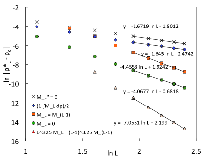
Figure 7: Convergence of estimates for $p_{c}$ based upon $M_{L}(p)$ assuming the critical value $p_{c}=0.5927460508$. We plot $\ln|p^{\star}_{L}-p_{c}|$ vs. $\ln L$, where $p^{\star}_{L}$ denotes the corresponding estimate for systems of size $L\times L$.

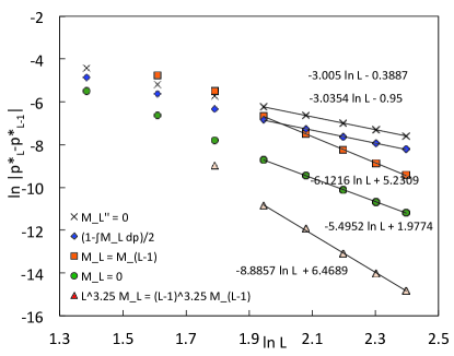
Figure 8: Convergence of various estimates for $p_{c}$ based upon $M_{L}(p)$ comparing systems of consecutive values of $L$. Here we plot $\ln|p^{\star}_{L}-p^{\star}_{L-1}|$ vs. $\ln L$.

V Conclusions

In conclusion we have shown that the classic Sykes-Essam matching-lattice formula can be generalized to an exact expression for finite lattices that relates the cluster numbers with various wrapping probabilities. The Sykes-Essam matching polynomial plays a key role in this general relation, and we show how to calculate it for both site and bond percolation. These considerations give a new perspective on the method developed by Scullard and Jacobson for finding thresholds accurately to high precision.

We have looked at the scaling of $M_{L}(p)$ and various threshold estimates $p^{\star}(L)$ based upon it. Assuming $2-x=3.25$, which corresponds to $w=4$, we find excellent scaling of the estimate determined by $L^{3.25}M_{L}(p^{\star})=(L-1)^{3.25}M_{L-1}(p^{\star})$, with an error of $\mathcal{O}(L^{-7})$, which is much smaller than for other threshold criteria. Whether this scaling applies to other lattices as well is an intriguing question for future research.

VI Acknowledgments

R. Z. acknowledges a pleasant visit and stimulating discussion with John Essam. S. M. thanks Cris and Rosemary Moore and Tracy Conrad for their hospitality and for inspiring discussions, and the Santa Fe Institute for financial support.

References

- Stauffer and Aharony (1994) D. Stauffer and A. Aharony, Introduction to Percolation Theory, 2nd ed. (Taylor & Francis, London, 1994).
- Grimmett (1999) G. R. Grimmett, Percolation, 2nd ed., Grundlehren der mathematischen Wissenschaften, Vol. 321 (Springer-Verlag, Berlin, 1999).
- Sykes and Essam (1964) M. F. Sykes and J. W. Essam, Journal of Mathematical Physics 5, 1117 (1964).
- Neher et al. (2008) R. A. Neher, K. Mecke, and H. Wagner, Journal of Statistical Mechanics: Theory and Experiment , P01011 (2008).
- Scullard and Jacobsen (2012) C. R. Scullard and J. L. Jacobsen, Journal of Physics A: Mathematical and Theoretical 45, 494004 (2012).
- Richeson (2008) D. S. Richeson, Euler’s Gem (Princeton University Press, Princeton and Oxford, 2008).
- Newman and Ziff (2001) M. E. J. Newman and R. M. Ziff, Physical Review E 64, 016706 (2001).
- Wu (2006) F.-Y. Wu, Physical Review Letters 96, 090602 (2006).
- Chayes and Lei (2006) L. Chayes and H. Lei, Journal of Statistical Physics 122, 647 (2006).
- Ziff and Scullard (2006) R. M. Ziff and C. R. Scullard, Journal of Physics A: Mathematical and General 49 (2006).
- Wierman and Ziff (2011) J. C. Wierman and R. M. Ziff, Electronic Journal of Probability 18, P61 (2011).
- Bollobás and Riordan (2010) B. Bollobás and O. Riordan, in An Irregular Mind, edited by G. F. Tóth et al. (Springer-Verlag, Berlin Heidelberg, 2010) pp. 131–217.
- Ziff (2006) R. M. Ziff, Physical Review E 73, 016134 (2006).
- Scullard (2006) C. R. Scullard, Physical Review E 73, 016134 (2006).
- Bollobás and Riordan (2006) B. Bollobás and O. Riordan, Percolation (Cambridge University Press, 2006).
- Jacobsen (2014) J. L. Jacobsen, Journal of Physics A: Mathematical and Theoretical 47, 135001 (2014).
- Jacobsen (2015) J. L. Jacobsen, Journal of Physics A: Mathematical and Theoretical 48, 454003 (2015).
- Mertens et al. (2016) S. Mertens, I. Jensen, and R. M. Ziff, “Cluster numbers in percolation,” arXiv:1602.00644, submitted (2016).
- Yang et al. (2013) Y. Yang, S. Zhou, and Y. Li, Entertainment Computing 4, 105 (2013).
- Feng et al. (2008) X. Feng, Y. Deng, and H. W. J. Blöte, Physical Review E 78, 031136 (2008).