Spatial Global Sensitivity Analysis of High Resolution classified topographic data use in 2D urban flood modelling

Abstract

This paper presents a spatial Global Sensitivity Analysis (GSA) approach in a 2D shallow water equations based High Resolution (HR) flood model. The aim of a spatial GSA is to produce sensitivity maps which are based on Sobol index estimations. Such an approach allows to rank the effects of uncertain HR topographic data input parameters on flood model output. The influence of the three following parameters has been studied: the measurement error, the level of details of above-ground elements representation and the spatial discretization resolution. To introduce uncertainty, a Probability Density Function and discrete spatial approach have been applied to generate $2,000$ DEMs. Based on a 2D urban flood river event modelling, the produced sensitivity maps highlight the major influence of modeller choices compared to HR measurement errors when HR topographic data are used, and the spatial variability of the ranking.
Keywords Urban flood; uncertainties; Shallow water equations; FullSWOF_2D; Sensitivity maps; Photogrammetry; classified topographic data.

Highlights

• Spatial GSA allowed the production of Sobol index maps, enhancing the relative weight of each uncertain parameter on the variability of calculated output parameter of interest.

• The Sobol index maps illustrate the major influence of the modeller choices, when using the HR topographic data in 2D hydraulic models with respect to the influence of HR dataset accuracy.

• Added value is for modeller to better understand limits of his model.

• Requirements and limits for this approach are related to subjectivity of choices and to computational cost.

Softwares availability

$$\begin{array}[]{|c|c|c|}\cline{1-3}\cr\text{ {\tiny Name of softwares}}&\text{{\tiny FullSWOF\_2D}}&\text{{\tiny Prom\'{e}th\'{e}e}}\\ \hline\cr\text{{\tiny Developers}}&\begin{array}[]{c}\text{{\tiny F. Darboux, O. Delestre,}}\\ \text{{\tiny C. Laguerre, C. Lucas, M.H. Le}}\end{array}&\text{{\tiny IRSN}}\\ \hline\cr\text{{\tiny Contacts}}&\text{{\tiny\url{fullswof.contact@listes.univ-orleans.fr}}}&\text{{\tiny\url{Yann.richet@irsn.fr}}}\\ \hline\cr\text{{\tiny First year of availibility}}&\text{{\tiny 2011}}&\text{{\tiny 2009}}\\ \hline\cr\text{{\tiny Operating system}}&\text{{\tiny Linux, Windows and Mac}}&\text{{\tiny Linux, Windows and Mac}}\\ \hline\cr\text{{\tiny Software availibility}}&\text{{\tiny\url{https://sourcesup.renater.fr/}}}&\text{{\tiny\url{http://promethee.irsn.fr}}}\\ \hline\cr\text{{\tiny Cost}}&\begin{array}[]{c}\text{{\tiny Free of charge, distributed under}}\\ \text{{\tiny CeCILL-V2 license (GPL compatible)}}\end{array}&\text{{\tiny Free of charge}}\\ \hline\cr\end{array}$$

1 Introduction

In hydraulics, deterministic numerical modelling tools based on approximating solutions of the 2D Shallow Water Equations (SWE) system are commonly used for flood hazard assessment [Gourbesville, 2015]. This category of tools describes water free surface behavior (mainly elevation and discharge) according to an engineering conceptualization, aiming to provide to decision makers information that often consists in a flood map of maximal water depths. As underlined in [Cunge, 2014], good practice in hydraulic numerical modelling is for modellers to know in detail the chain of concepts in the modelling process and to supply to decision makers possible doubts and deviation between what has been simulated and the reality. Indeed, in considered SWE based models, sources of uncertainties come from ($i$) hypothesis in the mathematical description of the natural phenomena, ($ii$) numerical aspects when solving the model, ($iii$) lack of knowledge in input parameters and ($iv$) natural phenomena inherent randomness. Errors arising from $i$, $ii$ and $iii$ may be considered as belonging to the category of epistemic uncertainties (that can be reduced e.g. by improvement of description, measurement). Errors of type $iv$ are seen as stochastic errors (where randomness is considered as a part of the natural process, e.g. in climatic born data) [Walker et al., 2003]. At the same time, the combination of the increasing availability of High Resolution (HR) topographic data and of High Performance Computing (HPC) structures, leads to a growing production of HR flood models [Abily et al., 2013, Erpicum et al., 2010, Fewtrell et al., 2011, Hunter et al., 2008, Meesuk et al., 2015]. For non-practitioner, the level of accuracy of HR topographic data might be erroneously interpreted as the level of accuracy of the HR flood models, disregarding uncertainty inherent to this type of data use, not without standing the fact that other types of above mentioned errors occur in hydraulic modelling.

1.1 High Resolution topographic data and associated errors

Topographic data is a major input for flood models, especially for complex environment such as urban and industrial areas, where a detailed topography helps for a better description of the physical properties of the modelled system [Abily et al., 2013, Djordjević et al., 2013, Gourbesville, 2015]. In the case of an urban or industrial environment, a topographic dataset is considered to be of HR when it allows to include in the topographic information the elevation of infra-metric elements [Le Bris et al., 2013]. These infra-metric elements (such as sidewalks, road-curbs, walls, etc.) are features that influence flow path and overland flow free surface properties. At megacities scale, HR topographic datasets are getting commonly available at an infra-metric resolution using modern gathering technologies (such as LiDAR, photogrammetry) through the use of aerial vectors like unmanned aerial vehicle or specific flight campaign [Chen et al., 2009, Meesuk et al., 2015, Musialski et al., 2013, Nex and Remondino, 2013, Remondino et al., 2011]. Moreover, modern urban reconstruction methods based on features classification carried out by photo-interpretation process, allow to have high accuracy and highly detailed topographic information [Andres, 2012, Lafarge et al., 2010, Lafarge and Mallet, 2011, Mastin et al., 2009]. Photo-interpreted HR datasets allow to generate HR DEMs including classes of impervious above ground features [Abily et al., 2014]. Therefore generated HR DEMs can include above ground features elevation information depending on modeller selection among classes. Based on HR classified topographic datasets, produced HR Digital Elevation Model (DEM) can have a vertical and horizontal accuracy up to $0.1\;\text{m}$ [Fewtrell et al., 2011].

Even though being of high accuracy, produced HR DEMs are assorted with the same types of errors as coarser DEMs. Errors are due to limitations in measurement techniques and to operational restrictions. These errors can be categorized as: ($i$) systematic, due to bias in measurement and processing; ($ii$) nuggets (or blunder), which are local abnormal value resulting from equipment or user failure, or to occurrence of abnormal phenomena in the gathering process (e.g. birds passing between the ground and the measurement device) or ($iii$) random variations, due to measurement/operation inherent limits (see [Fisher and Tate, 2006, Wechsler, 2007]). Moreover, the amount of data that composes a HR classified topographic dataset is massive. Consequently, to handle the HR dataset and to avoid prohibitive computational time, hydraulic modellers make choices to integrate this type of data in the hydraulic model, possibly decreasing HR DEM quality and introducing uncertainty [Tsubaki and Kawahara, 2013, Abily et al., 2015]. As recalled in the literature [Dottori et al., 2013, Tsubaki and Kawahara, 2013], in HR flood models, effects of uncertainties related to HR topographic data use on simulated flow is not yet quantitatively understood.

1.2 Uncertainty and Sensitivity Analysis

To evaluate uncertainty in deterministic models, Uncertainty Analysis (UA) and Sensitivity Analysis (SA) have started to be used [Saltelli et al., 2000] and [Saltelli et al., 2008] and become broadly applied for a wild range of environmental modelling problems [Refsgaard et al., 2007, Uusitalo et al., 2015]. UA consists in the propagation of uncertainty sources through model, and then focuses on the quantification of uncertainties in model output allowing robustness to be checked [Saint-Geours, 2012]. SA aims to study how uncertainty in a model output can be linked and allocated proportionally to the contribution of each input uncertainties. Both UA and SA are essential to analyze complex systems [Helton et al., 2006, Saint-Geours et al., 2014], as study of uncertainties related to input parameters is of prime interest for applied practitioners willing to decrease uncertainties in their models results [Iooss, 2011].

In 1D and 2D flood modelling studies, approaches based on sampling based methods are becoming used in practical applications for UA. For SA, depending on applications and objectives, different categories of variance based approaches have been recently applied in flood modelling studies (mainly in 1D) such as Local Sensitivity Analysis (LSA) [Delenne et al., 2012] or more recently, a Global Sensitivity Analysis (GSA) based on a screening method has been implemented in 2D flood modelling application [Willis, 2014].

Local Sensitivity Analysis

LSA focuses on fixed point in the space of the input and aims to address model behavior near parameters nominal value to safely assume local linear dependences on the parameter. LSA can use either a differentiation or a continuous approach [Delenne et al., 2012]. LSA based on differentiation approach performs simulations with slight differences in a given input parameter and computes the difference in the results variation, with respect to the parameter variation. LSA based on continuous approach differentiates directly the equations of the model, creating sensitivity equation [Delenne et al., 2012]. The advantages of LSA approaches are that they are not resource demanding in terms of computational cost, drawback being that the space of input is locally explored assuming linear effects only. Linear effects means that given change in an input parameter introduces a proportional change in model output, in opposition to nonlinear effects. LSA approaches perform reasonably well with SWE system even if nonlinear effects occur punctually (see [Delenne et al., 2012]). Nonetheless, important nonlinear effects in model output might arise when parameters are interacting and when solution becomes discontinuous. LSA consequently becomes not suited [Delenne et al., 2012, Guinot et al., 2007] in such a context, which is likely to occur in case of 2D SWE based simulation of overland flow.

Global Sensitivity Analysis

GSA approaches rely on sampling based methods for uncertainty propagation, willing to fully map the space of possible model predictions from the various model uncertain input parameters and then, allow to rank the significance of the input parameter uncertainty contribution to the model output variability [Baroni and Tarantola, 2014]. GSA approaches are well suited to be applied with models having nonlinear behavior and when interaction among parameters occurs [Saint-Geours, 2012]. These approaches going through an intensive sampling are computationally demanding, as they most often rely on Monte-Carlo (MC) approach, even though some more parsimonious sampling method such as Latin hypercube or pseudo-Monte Carlo are sometimes applied (see [Helton et al., 2006] for a review). Most commonly, GSA approaches rely on:

• screening methods, such as Morris method [Morris, 1991];

• Sobol indices computation, that considers the output hyperspace ($x$) as a function ($Y(x)$) and performs a functional decomposition [Iooss, 2011, Iooss and Lemaître, 2015] or a Fourier decomposition (FAST method) of the variance.

As fully detailed in [Iooss and Lemaître, 2015], screening techniques (e.g. Morris method) allow to classify uncertain input parameters in three categories: those that have negligible effect; those that have linear effect; and those that have nonlinear effects or effects in interaction with other input parameters. Sobol indices (or variance-based sensitivity indices) will explain the share of the total variance in the space of output due to each uncertain input parameter and/or input interaction.

GSA has started to be applied in 1D hydraulic modelling in practical applications for hierarchical ranking of uncertain input parameters [Alliau et al., 2015, Hall et al., 2005, Jung and Merwade, 2015, Nguyen et al., 2015, Pappenberger et al., 2008]. As for 1D, applying a GSA to flooding issues in 2D modelling requires method awareness among the community, practical tools development and computational resources availability. Moreover an analysis on spatialization of input uncertain parameters and on output variable is specifically needed in 2D [Saint-Geours et al., 2011]. Recently, GSA using a screening method has been implemented in 2D flood modelling application [Willis, 2014] tackling ranking of uncertain input parameters using points and zonal approaches. Computation of sensitivity maps such as maps of Sobol index is a promising outcome that has been achieved for other types of water related issues [Marrel et al., 2011].

1.3 Objectives of the study

To date, UA and SA have not yet been performed to specifically study uncertainty in 2D urban flood simulations related to HR classified topographic data integration. Indeed, due to the curse of dimensionality, SA methods have seldom been applied to environmental models with both spatially distributed inputs and outputs [Saint-Geours et al., 2014]. Such a problematic raises needs of specific tools, computational resource and methods application. Among SA methods, a Global Sensitivity Analysis (GSA) is implemented in this study. GSA approach is selected over LSA as 2D overland flow process simulation through SWE system of partial differential equations, is viewed as being largely nonlinear, with discontinuous solution and interactions between parameters.

This paper aims to study uncertainty related to HR topographic data integration in 2D flood modelling approach. The objective of the study is to perform an UA and a SA on two categories of uncertain parameters (measurement errors and uncertainties related to operator choices) relative to the use of HR classified topographic data in a 2D urban flood model having spatial inputs and outputs. Among SA methods, a Global Sensitivity Analysis (GSA) is implemented to produce sensitivity maps based on Sobol index computation. Carrying out these objectives will demonstrate the feasibility, the added values and limitations of UA and SA implementation in 2D hydraulic modelling, in a context where spatial variability and interaction are likely to occur. Moreover, modeller knowledge about challenges and expectations related to HR classified data use in HR urban flood modelling will be enhanced.

The study case is the low Var river valley (Nice, France) where flooding events occurred in the last decades in the highly urbanized downstream part of the valley [Guinot and Gourbesville, 2003]. The output of interest is the overland flow water level ($Y(x)$). The used HR DEMs are based on classified 3D dataset created from photointerpretation procedure. A proof of concept of GSA application to 2D Hydraulic modelling voluntary choosing a resource requiring problem has been developed and the method applied over an innovative concern related to the use of HR topographic data.

Following this introduction (Part 1) , the next part of the paper (Part 2) introduces the test case context for SA methods uses, then enhances description of used HR topographic dataset, gives overview of implemented methodology for the spatial GSA and introduces developed tools. The third part (3) of the paper presents results of UA and GSA, first at punctual then at spatial levels. The last parts (Part 4 and 5) discuss outcomes and limits of our approach, providing concluding remarks.

2 Method

The study area is a $17.8\;\text{km}^{2}$ domain that represents the last five downstream kilometers of the low Var valley, located in Nice, France (figure 1). In the test basin, two major river flood events occurred in last decades ($5^{th}$ of November $1994$; $6^{th}$ of November $2011$). A HR topographic data gathering campaign fully covered the domain in $2010-2011$. The characteristics of the river basin and of the $1994$ flood event are described in [Guinot and Gourbesville, 2003]. Between $1994$ and $2010-2011$ (date of event used for simulation and the date of the HR topographic data gathering campaign), the studied area has considerably changed. Indeed, levees, dikes and urban structures have been implemented, changing physical properties of the river/urban flood plain system. Thus, the objective is not to reproduce the event, but simply to use the framework of this event as a case study to carry out the UA and the SA. As mentioned in the introduction section, a GSA approach using Sobol index is suitable to compute sensitivity maps [Marrel et al., 2011]. The method implemented to carry out the spatial GSA is presented in detail in [Abily et al., 2015], and the upcoming description of the implemented GSA gives to the reader a summary of key elements for understanding.

2.1 HR classified topographic data and case study

The design and the quality of a photo-interpreted dataset are highly dependent on photogrammetry dataset quality, on classes’ definition, and on method used for digitalization of vectors [Lu and Weng, 2007]. Reader can find details regarding principle of modern aerial photogrammetry technology in [Egels and Kasser, 2004]. The photogrammetric campaign carried out over the lower Var valley, at a low flight elevation, allowed a pixel resolution at the ground level of $0.1\;\text{m}$ and had a high overlapping ratio ($80\%$) among aerial pictures. Consequently, these characteristics allowed the production of a high quality photogrammetric dataset. Using the photogrammetric dataset, the photo-interpretation process has been carried out, to create a classified vectorial dataset through digitalization of classes of polylines, polygons and points. This photo-interpreted dataset has been designed with a total number of $50$ different classes representing large and thin above ground features (e.g. buildings, concrete walls, road-gutters, stairs, etc.). The specificities of the given photo-interpretation process can be found in [Andres, 2012]. For hydraulic modelling purpose, $12$ classes over the $50$ are considered to represent above ground features impacting overland flow path, as shown in figure 1 (a, b).

Classified data mean horizontal and vertical accuracy is $0.2\;\text{m}$. Errors in photo-interpretation which results from feature misinterpretation, addition or omission are estimated to represent $5\%$ of the total number of elements. To control average level of accuracy and level of errors in photo-interpretation, the municipality has carried out a terrestrial control of data accuracy over $10\%$ of the domain covered by the photogrammetric campaign.

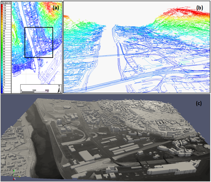
Figure 1: Overview of the classes of photo-interpreted topographic data uses over the study area (a, b) and HR DEM of a sub-part of interest of the domain (c).

For our application, the 3D classified data of the low Var river valley is used to generate specific DEM adapted to surface hydraulic modelling. For the GSA approach (see next section), only the input DEM changes from one simulation to another and the hydraulic parameters of the model are set identically for the simulations. Hydraulic conditions of the study case implemented in the models can be summarized as follow: a constant discharge of $1,500\;\text{m}^{3}.\text{s}^{-1}$ is applied as input boundary condition to reach a steady flow state condition almost completely filling the Var river bed. This steady condition is the initial condition for the GSA and a $6$ hours estimated hydrograph from the $1994$ flood event is simulated [Guinot and Gourbesville, 2003]. The Manning’s friction coefficient ($n$) is spatially uniform on overland flow areas with a standard value of $0.015$, which corresponds to a concrete surface. No energy losses properties have been included in the 2D hydraulic model to represent the bridges, piers or weirs. Downstream boundary condition is an open sea level (Neumann boundary condition) to let water flows out.

2.2 Spatial GSA approach

Falling within category of GSA approaches, screening methods allow in a computationally parsimonious way, to discriminate among numerous uncertain input parameters those that have little effect from those having linear, nonlinear or combined effects in output variance [Iooss and Lemaître, 2015]. Screening methods principle consists in fixing an input parameters set and performing an initial run. Then, for one parameter at a time, a new value of the parameter is randomly chosen and a new run is performed. Variation in the run output is checked. This operation is completed for all the parameters, $n$ times with $n$ equals to the total number of input parameters. Screening methods perform well to discriminate influencing parameters on output variability with 2D flood modelling studies [Willis, 2014].
GSA approaches relying on Sobol index computation go one step further, allowing to quantify the contribution to the output variance of the main effect of each input parameters [Sobol’, 1990, Saltelli et al., 1999, Saint-Geours, 2012]. Sobol Index is based on functional decomposition of variance (ANOVA), considering $Y$ the model output of interest as follow: $Y=f(X)$; where $f$ is the model function, $X=(X_{1};...;X_{i})$ are $i$ independent input uncertain parameters with known distribution. Sobol indices ($S_{i}$) of parameter $X_{i}$ are defined as:

$${S_{i}}_{(X_{i})}=Var\left[\mathbb{E}(Y|X_{i})\right]/Var(Y),$$ (1)

where $\mathbb{E}$ is the expectation operator. ${S_{i}}_{(X_{i})}$ being the variance of conditional expectation of $Y$ for $X_{i}$ over the total variance of $Y$, ${S_{i}}_{(X_{i})}$ value will range between $\left[0;1\right]$. $S_{i}$ computations are computationally costly as it requires to explore the full space of inputs and therefore an intensive sampling is necessary [Iooss and Lemaître, 2015].

Objective being to quantify impacts of input parameters, GSA approach using Sobol index is best suited for sensitivity maps production. In this study, the implemented GSA follows standard steps used for such type of approach as summarized in [Baroni and Tarantola, 2014] or in [Saint-Geours et al., 2014].

The steps of the method are presented in the figure 2: specification of the problem notably by choosing uncertain parameters and output of interest (step A); assessing Probability Density Function (PDF) of uncertain parameters (step B); propagating uncertainty, using a random sampling approach in our case (step C); ranking the contribution of each input parameters regarding the output variance (step D).

First steps of the approach (A and B) are the most subjective ones. For the study purpose, steps A and B are treated as follow. Three input parameters related to uncertainties when willing to use HR 3D classified data in 2D Hydraulic models are ($i$) one parameter related to the topographic input error (called var. $E$) and ($ii$) two parameters related to modeller choices, when including HR data in 2D hydraulic code (called var. $S$ and var. $R$) are considered in this GSA practical case. These three parameters are considered as independent.

First, the uncertainties related to measurement errors in HR topographic dataset are considered through var. $E$. This parameter is an error randomly introduced for every point of the highest resolution DEM ($1\;\text{m}$) following a draw according to a normal distribution PDF, where the standard deviation is equal to the RMSE value $\left(0.2\;\text{m}\right)$: $\mathcal{N}(0,0.2)$. As from one point to the next one, the normal PDF is drawn independently, it results in a spatialization that follows a uniform distribution. Hundred maps of var. $E$ are generated and combined with the ($1\text{m}$) resolution DEMs.

Then, for uncertainties related to modeller choices when including HR data in hydraulic code, two variables are considered: var. $S$ and var. $R$.

Var. $S$ is a categorical ordinal parameter having values representing the level of above ground features details impacting flow direction included in DSM. $S1$ is a DTM (Digital Terrain Model) only, $S2$ is $S1$ combined with buildings elevation inclusion, $S3$ is $S2$ completed with walls, and $S4$ is $S3$ plus thin concrete structures (sidewalks, roar-curbs, etc.).

Var. $R$ represents choices made by the modeller concerning the computational grid cells resolution in the model. In the hydraulic code used for this study (FullSWOF_2D described in next subsection), the grid cells are regular. This parameter var. $R$ can have five discrete values from $1\;\text{m}$ to $5\;\text{m}$. At 1m resolution, number of computational points of the grid is above $17.5$ million and at the $5\;\text{m}$ resolution grid size is $700,000$ computational points. The bounding of this parameter is justified as on one hand, a grid resolution lower than $1\;\text{m}$ would result in prohibitive computational time. On the other hand, resolutions coarser than $5\;\text{m}$ do not sound to be a relevant choice for a modeller willing to create a HR model, as up-scaling effects would make the use of the HR topographic data that are used as input irrelevant.

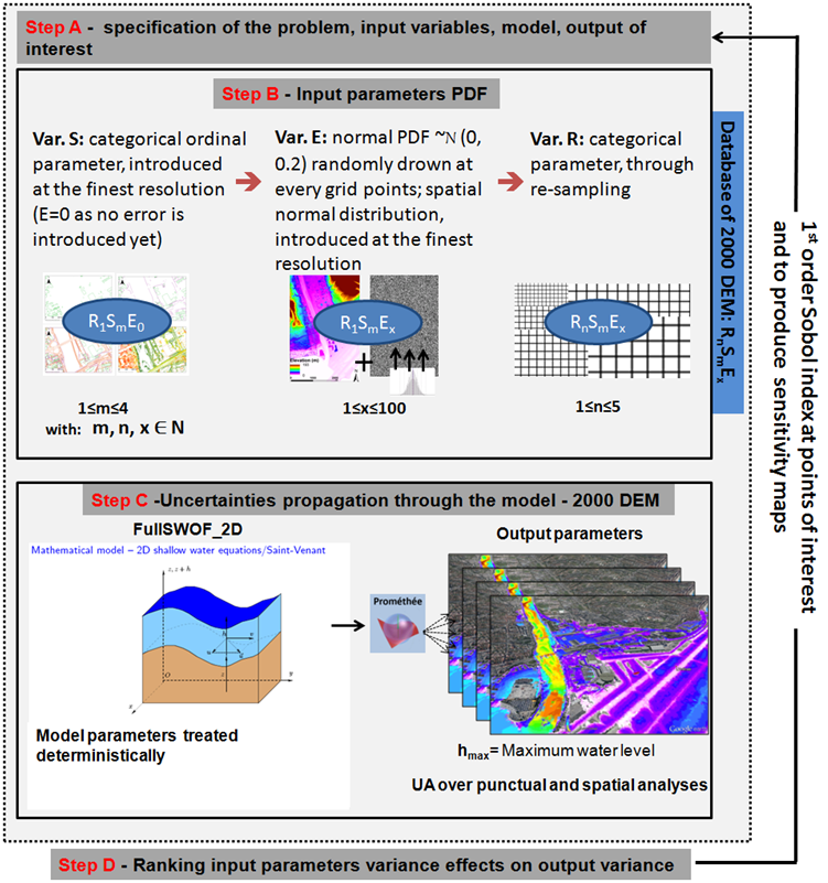
Figure 2: Overview of the applied spatial GSA framework.

A total of $2,000$ DEMs are generated and used in the implementation of the GSA. The DEMs generation process (step B, figure 2), explains as follow. Four DEMs at the finest resolution (var. $R=1\;\text{m}$) are generated to implement all of the four var. $S$ possible scenarios. Then each of these four DEMs is combined with the hundred var. $E$ grids producing $400$ DEMs. Eventually, the $400$ DEMs combining all of the var. $S$ and var. $E$ possibilities combinations are resampled to resolution $2,\;3,\;4,\;5\;\text{m}$ creating a database of $2,000$ DEMs where all the defined input parameters can possibly be combined.

The propagation of uncertainty (step C) is carried out using a MC approach to randomly sample in the database. Non-parsimonious approach consisting in computing a maximum number of simulations among the $2,000$ possible cases has been carried out to generate a database of results. In total, $1,500$ simulations out of the $2,000$ possible were computed to feed the result database using the available $400,000$ CPU hours on a Cluster (cluster described in next sub-section). Therefore, to make sure that the input space would be extensively explored, for all of the $20$ possible var. $R$/ var. $S$ combinations, at least $50$ over the $100$ possible var. $E$ drawn were performed. As the exploration of the space of input is restricted to $1,500$ simulations over $2,000$ possible cases, an evaluation of the convergence is performed to assess if the convergence of the MC method is reached. Figure 3 illustrates the evolution of the convergence of the mean of the hyperspace of the output of interest $Y(x)$ for three points (points located in figure 4), increasing $N$ through a random sampling in the result database. It is reminded here that the output of interest is the simulated maximal overland flow water depth. An asymptotic convergence of the MC method is observed for the three points, respectively when the sample size ($N$) is larger to $900$ simulations. Globally, over the 20 selected points, when N reaches a threshold value between $900-1000$, the stabilization of the convergence is observed.

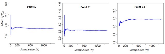
Figure 3: Asymptotic convergence of random sampling at $3$ points of interest (points $5$, $7$ and $14$ located on figure 4).

Step D consists in the computation of Si using the output database. Sobol index of var. $R$, var. $S$ and var. $R$, respectively $S_{i}(R)$, $S_{i}(S)$ and $S_{i}(E)$ are computed following Eq. (1) at points of interests. Spatialization of GSA approach is based on discrete realization of spatially distributed input variables as described in [Lilburne and Tarantola, 2009], and discrete computation of output to produce sensitivity maps (as described in [Marrel et al., 2011]).

2.3 Parametric environment and 2D SWE relying code

Prométhée (a parametric modelling environment), has been coupled with FullSWOF_2D (a 2D free surface modelling code) over a High Performance-Computing (HPC) structure [Abily et al., 2015].

Prométhée is an environment for parametric computation that allows carrying out uncertainties propagation study, when coupled (or warped) to a code. This software is freely distributed by IRSN (http://promethee.irsn.org/doku.php). Prométhée allows the parameterization with any numerical code and is optimized for intensive computing. Moreover, statistical post-treatment, such as UA and SA can be performed using Prométhée as it integrates R statistical computing environment [Ihaka, 1998].

FullSWOF_2D (for Full Shallow Water equation for Overland Flow in 2 dimensions) is a code developed as free software based on 2D SWE [Delestre et al., 2012, Delestre et al., 2014]. Two parallel versions of the code have been developed allowing to run calculations under HPC structures [Cordier, S. et al., 2013]. In FullSWOF_2D, the 2D SWE are solved using a well-balanced finite volume scheme based on the hydrostatic reconstruction (see [Audusse et al., 2004, Delestre et al., 2014]). The finite volume scheme is applied on a structured spatial discretization using regular Cartesian meshing. For the temporal discretization, based on the CFL criterion, a variable time step is used. The hydrostatic reconstruction (which is a well-balanced numerical strategy) allows to ensure that the numerical treatment of the system preserves water depth positivity and does not create numerical oscillation in case of a steady states, where pressures in the flux are balanced with the source term here (topography). Different solvers can be used HLL, Rusanov, Kinetic [Bouchut, 2004], VFRoe-ncv combined with first order or second order (MUSCL or ENO) reconstruction. The HLL solver has been used in this study with a first order MUSCL reconstruction method.

On the HPC structure (Interactive Computation Centre of Nice Sophia Antipolis University), up to $1152$ CPUs are available and up to $30$ simulations can be launched simultaneously using Prométhée-FulSWOF_2D. A database of flood maps results has been produced using a total of $400,000$ CPU hours. The required unitary computation time is two hours over $64$ CPUs, for simulations using the finest resolution grid size ($1\;\text{m}$), which has $17.8$ millions of computational points. At the coarsest resolution ($5\;\text{m}$), the grids size is decreased to $712,000$ computational points and using $64$ CPUs, the computational time decreases to few minutes.

3 Results

This section presents the results of the UA and the GSA. A subarea is selected in the flooded area of the domain to carry out the spatial analysis. This subarea is $4.35\;\text{km}^{2}$, representing one quarter of the total spatial extent of the model. $20$ points of interest are defined in the selected flooded area of the subarea (figure 4). Points $1$ to $10$ are spread in and around the main streets. These streets are densely urbanized. Points $11$ to $16$ are located in less urbanized areas (stadium, parking, small agricultural field, etc.). Moreover, from points $15$ to $20$, points are located in areas which are at the edge of the flood extent, either in open area (points $15$ and $16$) or where above ground features are densely present (points $17$ to $20$).

3.1 Uncertainty analysis

Punctual view

Mean and variance of computed maximal water depth ($Y(x)$) at the different points of interest are presented in figure 4. Means and standard deviations of $Y(x)$ values are computed using the full size database ($N=1,500$). Over the $20$ points of interest, importance of the variability introduced by uncertain input parameter is significant ($0.51\;\text{m}$ in average). Moreover, variability in $Y(x)$ variance can be important as the minimal variance is $0.28\;\text{m}$ (point $17$), and the maximal variance is $0.71\;\text{m}$ (point $8$). Further interpretation, such as the analysis of the trend in the magnitude of variance changes from one point to another, is not accessible for generalization using punctual observation only. Nevertheless, studying the distribution of $Y(x)$ at points of interest gives another insight to carry out the uncertainty analysis.

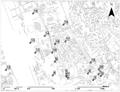
Figure 4: Location of points of interest and associated values.

Figure 5 illustrates $Y(x)$ distributions using the complete set of available model runs in the database for three points. $Y(x)$ follows a normal distribution, as observed for point $7$ or distribution can be bi-modal as observed for point $14$. The difference between the normal and bi-modal distribution of $Y(x)$ is not always clearly observed (point $5$). Most of the clearly observed bimodal distribution (ten out of the twenty points) occurs for the points located in the central part of the highly urbanized area (points $1$ to $10$). This area is largely flooded, and seven points have here a clearly marked bimodal distribution. In largely flooded but relatively less urbanized areas, the trend is reversed as five out of six points have a normal distribution. Lastly for the points located at the edge of the flooded areas, two over four points have a bimodal distribution, whereas the two others have a normal one. Bimodal distributions lead to larger amplitude in $Y(x)$ distribution. The bimodal distribution illustrates the non–linearity between the input and output. Explanations to link these observations with physical properties of phenomena and of uncertain input parameter properties are given, combining these observations with SA results, in the discussion section. Moreover, it is noticeable that points are sometimes not flooded at all, when $Y(x)$ is equal to zero. Reasons for these zero values are that in seldom cases, var. $E$ value gives at the point of interest a high ground elevation value (above $Y(x)$ value) or that var. $S$ produces critical threshold effects diverting flow direction.

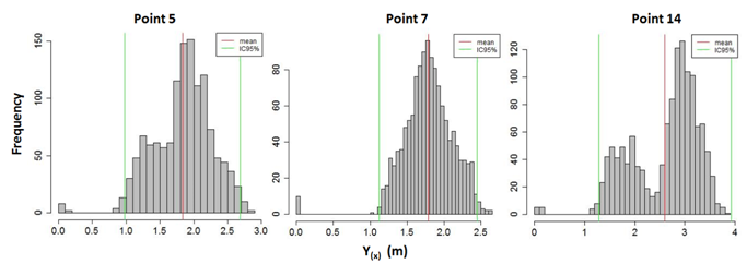
Figure 5: Distribution of $Y(x)$ at three points of interest (points, located on figure 4).

Spatial analysis

The comparison of maps of $Y(x)$ mean and variance (figure 6) puts to the light the fact that areas densely urbanized and having a high water depths, have a high variance in $Y(x)$. This maps comparison also underlines the fact that areas having a high mean water depths in less densely urbanized, and in areas close to the edge of flood spatial extent (having a smaller mean water depth) have a lower variance value of $Y(x)$. This confirms the local observations at points of interests. Moreover, a high variance of $Y(x)$ is observed in the map for places that have steep slope such as river bank, access roads, highway ramps or dikes. Intuition would lead to incriminate here resolution of discretization effects (var. $R$) as it will be confirmed by the SA (see next section and discussion part). Over the river, variance is locally important. The spatial changes in variance in the river bed ranges from $0.1\>\text{m}$ to $1\;\text{m}$. Amplitudes in variance in the river bed are most likely due to above ground features additions when var. $S$ changes (features such as walls, dikes levees, and roads elements in the main riverbed), that does change the width of the river bed itself. Consequently, these local important variance values are not surprising. Our study focuses on overland flow areas. A GSA over riverbed itself would be out of the range of the spatial GSA defined for this study.

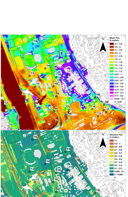
Figure 6: Maps of mean and variance values of $Y(x)$.

3.2 Variance based global sensitivity analysis

Flood event scenario

$1^{\text{st}}$ order Sobol index ($S_{i}$) of var. $S$ ($S_{i}(S)$), var. $R$ ($S_{i}(R)$) and var. $E$ ($S_{i}(E)$) are computed for the $20$ points of interest. Figure 7 (a) shows the evolution of computed $S_{i}$ increasing $N$ through a random sampling in the results database for the same three points used in the figure 5. Stabilization of the computed $S_{i}$ values is observed when $N$ is approximately $1,000$, confirming that convergence of the random sampling is reached around this $N$ value. It has to be noticed that below a value of $N=500~{}600$, the samples are too small to compute $S_{i}(E)$ with our algorithm (draws of var. $E$ are too scarcely distributed in the matrix to compute conditional expectation of var. $E$). A bootstrap is performed, to check confidence interval of the computed $S_{i}$ as can be seen in figure 7 (b). For each point, independent samples of size $N=1,000$ are randomly drawn $10,000$ times in the results data base to compute $10,000$ times $S_{i}$. Then the $S_{i}\;95\%$ confidence interval is computed.

Over the $20$ selected points, the average $S_{i}(S)$ value is $0.40$, the average $S_{i}(R)$ value is $0.24$ and the average $S_{i}(E)$ value is $0.06$. $S_{i}(S)$ is ranked as the highest among the three $S_{i}$ for $13$ out of the $20$ points. For the seven other points, $S_{i}(R)$ is ranked as the highest $S_{i}$. The results show that Var. $E$ is never the variable which influences the most $Y(x)$ variance and $S_{i}(E)$ is ranked as the second highest $S_{i}$ only for points $15$ and $16$. These points are located at the edge of the flood extent area where the $Y(x)$ values are in average below $1\;\text{m}$.

For the $20$ points, the difference between the highest ranked $S_{i}$ and the second one is often clear (around $0.35$), but the difference between the $S_{i}$ ranked as $2^{\text{nd}}$ and $3^{\text{rd}}$ is often not important (around $0.1$) and can be smaller than the $95\%$ confidence interval calculated from the bootstrap.

The main outcome from the punctual GSA is that var. $S$ and var. $R$, which are two modeller choices when including HR topographic data in the model, are always the parameters contributing the most to $Y(x)$ variance. The analysis also highlights that var. $E$ does not introduce much variance on $Y(x)$. For the $20$ points, $S_{i}$ ranking varies from one point to another one, enhancing the spatial variability of uncertain parameters influence on $Y(x)$ variance and strengthening the interest of sensitivity maps production.

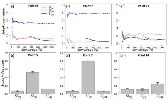
Figure 7: Illustration for three points of interest of Sobol indices convergence (a, a’, a”) and of confidence interval computed using bootstrap method (b, b’, b”).

Spatial analysis

Over the selected subarea, $S_{i}$ are computed every $5\;\text{m}$ to produce sensitivity maps. With this level of discretization, it represents a total of $120,000$ points where $S_{i}$ are calculated. A test has been carried out at a finer resolution ($1\;\text{m}$) over a $100\;\text{m}$ per $100\;\text{m}$ area for $S_{i}$ mapping. Results in $S_{i}$ maps at $1\;\text{m}$ and $5\;\text{m}$ are similar over this small area. Therefore, the $S_{i}$ maps are computed at a resolution $5\;\text{m}$ as the number of points to compute is $25$ times less important than for a $1\;\text{m}$ resolution. The $S_{i}$ are computed at every points using $N$ equal to the full size of available simulations in the results database ($1,500$).

A first analysis of the distribution of computed $S_{i}$ is illustrated in figure 8 (a). Non flooded areas are removed for this analysis as well as areas covered by buildings. Indeed, inside the buildings which are represented as impervious blocks in the model, $S_{i}(S)$ is equal to one. Therefore, var. $S$ explains the entire variance of $Y(x)$ in building areas. Moreover, at the edges of buildings, $S_{i}(R)$ is equal to one as well, due to buildings resolution effects. The number of points where $S_{i}$ have been calculated and that are plotted in figure 8 (a) is around $60,000$. The results show that:

• $S_{i}(S)$ is highly distributed around $0.1$ and has two peaks in distribution around $0.6$ and $0.75$ that have a flatter shape;

• $S_{i}(R)$ is highly distributed around a value of $0.25$. A second minor distribution peak around $0.60$; $S_{i}(E)$ distribution is a single peak centered in $S_{i}(E)=0.07$, which is a value lower than both $S_{i}(R)$ and $S_{i}(S)$ peaks.

Analysis of these multi-modal distributions, confirms punctual GSA results regarding the non-spatially homogeneous ranking of $S_{i}$. The analysis of $S_{i}$ maps will help to understand the spatial distribution and the ranking of uncertain input parameters according to their influence over the output variance.

Figure 8 (c) presents the Sobol index maps. Analyzing in the first place the maximal $S_{i}$ spatial distribution, it appears that, $S_{i}(R)$ and $S_{i}(S)$ are always ranked with the highest value. $S_{i}(R)$ is ranked as the highest over $67\%$ of the subarea whereas $S_{i}(S)$ is ranked as the highest over $32\%$ of the subarea. Var. $E$ is rarely the most impacting parameter. This confirms the punctual GSA results and the $S_{i}$ distribution analysis. In the second place, using the spatial repartition of $S_{i}$ values presented as sensitivity maps (figure 8 (b)), the following remarks arise:

• $S_{i}(s)$ is ranked as the highest index in locations where $Y(x)$ has a high variance. In the areas with a high $Y(x)$ variance, $S_{i}(s)$ values range between $0.3$ and $0.8$. Those high $S_{i}(s)$ areas are characterized by a highly urbanized environment where above ground features strongly impact $Y(x)$.

• $S_{i}(S)$ is ranked as the highest $S_{i}$, where a given above ground element strongly impact locally hydrodynamic and consequently $Y(x)$.

• $S_{i}(R)$ happens to be the most impacting parameters in areas less densely urbanized.

• Moreover, high ranking of $S_{i}(s)$ also occurs when a given aboveground structure impacts upstream or downstream calculation of $Y(x)$ whatever is the urban configuration/density of affected upstream or downstream areas.

• $S_{i}(R)$ is ranked as the highest $S_{i}$ when $Y(x)$ is low (below $1\;\text{m}$), and when in the meantime, variance of $Y(x)$ is low as well. It corresponds to areas close to the edge of the flood extent.

• $S_{i}(R)$ is ranked as the highest $S_{i}$ in areas which are less densely urbanized and where no above ground features, at the given area, neither upstream nor downstream, have any important effects on $Y(x)$.

• $S_{i}(R)$ is ranked as the highest $S_{i}$ in areas where the ground slope is steep. Indeed the level representation of a sloping area is highly affected locally by the degree of resolution of the discretization.

• $S_{i}(E)$ low and almost homogeneous over the subarea.

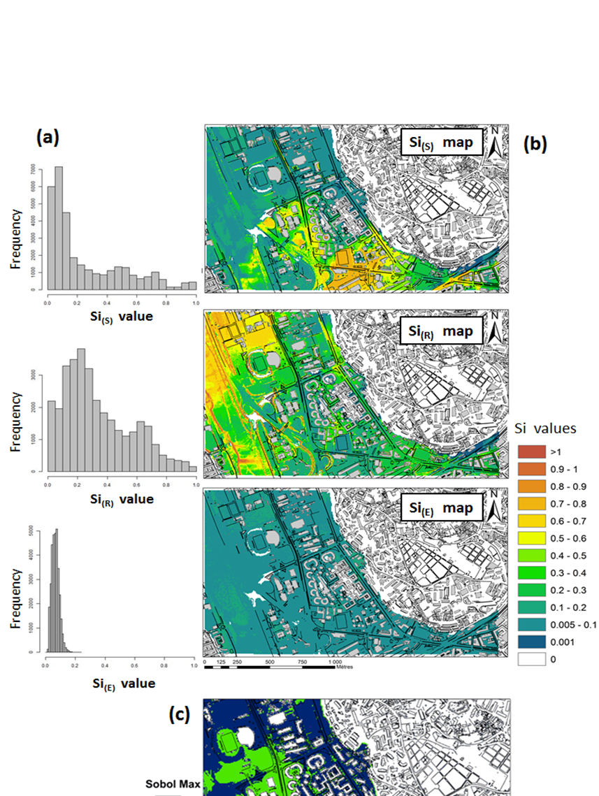
Figure 8: Distribution of computed $S_{i}$ (a), details of $S_{i}$ maps (b) and map of highest ranked $S_{i}$ (c).

4 Discussion

The Implemented approach is a proof of concept of applicability of spatially distributed GSA to 2D hydraulic problems. UA and spatial ranking of influent uncertain input parameters over the 2D HR flood modelling study case have been achieved. Nevertheless, being a first attempt, the approach can be improved. Outcomes, limits and perspectives are underlined in this section and compared with other research fields in geomatics, SA and hydraulic modelling.

4.1 Outcomes

A basic UA leads to the following conclusions on: output variability quantification, nonlinear behavior of the model and spatial heterogeneity. Within established framework for the UA, the considered uncertain parameters related to the HR topographic data accuracy and to the inclusion in hydraulic models influence the variability of $Y(x)$ in a range that can be up to $0.71\;\text{m}$. This stresses out the point that even though hydraulic parameters were set-up as constant, the uncertainty related to HR topographic data use cannot be omitted and needs to be assessed and understood. These warnings were already raised up in [Dottori et al., 2013] and [Tsubaki and Kawahara, 2013], and are strengthened in this study by $Y(x)$ variance quantification. The quantification is not easily transposable in other contexts and it is not an easy process to give general trend for practical applications given the fact that ($i$) spatial heterogeneity of $Y(x)$ variance is observed and ($ii$) specificities of different HR classified dataset is highly variable. Nevertheless, this quantification of uncertainty goes in the direction of improvement of state of the art as common practice is still to quantify uncertainty using expert opinion only (see [Krueger et al., 2012]). Investigations on the UA can lead to deeper understanding of mechanisms leading to $Y(x)$ variability. The punctual analyses of the $Y(x)$ distributions (either unimodal or multimodal) illustrate the nonlinearity of uncertain parameters effects over the output. This nonlinearity in the output distributions is most likely due to var. $S$ which represents the level of details of above ground features incorporated in HR DEMs.

Punctual SA highlighted that depending on location of considered point of interest, maximal first order $S_{i}$ are different. This goes in the direction of a need of spatial representation of $S_{i}$ under the form of sensitivity maps for consistent analyses. This spatial distribution of $S_{i}$ showed the major influence of the modeller choices when using the HR topographic data in 2D hydraulic models (var. $S$ and var. $R$) with respect to the influence of HR dataset accuracy (var. $E$). Hence as underlined in [Marrel et al., 2011], if one wants to reduce variability of $Y(x)$ at a given point of interest, the use of sensitivity maps helps to determine the most influential input at this point. Moreover, sensitivity maps give possibility to link the spatial distribution of $S_{i}$ to the properties of the model, especially with the physical properties of represented urban sector topography. The fact that var. $S$ is the most contributing parameter in densely urbanized areas is not surprising as it introduces a change in the representation in the model of physical properties of the urban environment. The var. $R$ indirectly impacts quality of small scale elements representation well.

4.2 Limits of the implemented spatial GSA approach

GSA allowed to compute sensitivity maps, but simplifications and choices, especially regarding the way step A (setting up of the spatial GSA framework by choosing uncertain parameters and choosing a way to spatialize them) and step B (assigning PDF to input parameters), lead to simplifications which are interesting to enhance.

For the uncertainties related to errors in HR topographic data (var. $E$), the followed Normal PDF having properties of the RMSE is randomly introduced, for every points of the highest resolution DEM ($1\;\text{m}$). Nevertheless, as from one point to the next one, the normal PDF is drawn independently, it results in a uniform spatial distribution. In practice a uniform repartition should increase entropy and maximize errors/uncertainties effects. In the present case, this consideration is not valid. Indeed, the used parameter is a RMSE which is already averaged over the space. In fact as reminded in [Wechsler, 2007], the RMSE is calculated based on assumption of normality which is often violated. For instance, over open and flat areas (e.g. parking, roads), relative accuracy from one point to another should increase. In the study case, a comparison with ground topographic data measurement revealed that accuracy of HR DEM RMSE increases to $0.05\;\text{m}$. Hence, over flat areas where the var. $E$ appears to be ranked as the second most contributing parameter to $Y(x)$ variability, not without standing the fact that the $S_{i}$ confidence interval of ranked second and third parameters overlaps, it sounds reasonable to think that var. $E$ is overestimated. Opposite effect is observable over sloping areas (e.g. dikes), where in our cases, after a regional control of the measurement quality, it is found that RMSE value is about $1\;\text{m}$. Therefore, especially over steep slope areas such as dikes where var. $R$ has been found to be the most important parameter contributing to $Y(x)$ variability, our $S_{i}$ ranking has to be taken with caution as var. $E$ has probably been locally underestimated. For further work, it would be interesting to improve the approach, by using spatialized value of RMSE in function of topographic properties. This regionalization of characteristics of PDF might not be easy to implement by practitioners as regional information of accuracy might not be available. In that case, basic assumption to attribute regionally different characteristics to PDF could be relevant. For var. $E$, a component related to photointerpretation errors should have been taken into consideration. Moreover, in order to improve our study, it would be relevant to include a new variable that would reflect errors in photointerpretation. Basically, this should consist in a random error in classified data for $5\%$ of the number of elements used for DEM generation. From a technically point of view, implementation of such process is not straight forward particularly, recalling that this study is a first proof of concept on the topic. Therefore, it has not been included in the SA. Nevertheless, errors in photo-interpretation, which are uncertainties inherent to the HR dataset would have locally a considerable impact on $Y(x)$ variability and would require further research.

For modeller choices, in terms of level of details in classified features to be integrated in the hydraulic models (var. $S$), it is reasonable to consider this parameter as a categorical ordinal parameter having a uniform PDF. Indeed, depending on availability of information of features influencing overland flow defined as classes and depending on model objective, modeller will select one of the available options in increasing complexity of DEM. The choice of a row HR DTM (without buildings, var. $S1$) is mostly responsible of the observed binomial distribution in the UA, leading to an under estimation of maximal water depth $Y(x)$ compare to other cases. Nevertheless it appears as well that punctually, at $1\;\text{m}$ and $3\;\text{m}$ resolutions, var. $S4$ leads to low $Y(x)$ value as well due to local effects over flow paths.

For modeller choices in terms of level of discretization (var. $R$), HR DEM were used, we constrained ourselves to resolution levels which are realistic with the use of such type of data considering that a resolution higher than $5\;\text{m}$ is not compatible with the idea of producing HR models. Nonlinear effects of resolution are long time known by practitioners in the sense that the grid resolution will impact the level of details included in the model [Horritt and Bates, 2001, Mark et al., 2004, Djordjević et al., 2013].

5 Summary and conclusions

Implemented approach is a proof of concept of applicability of spatially distributed variance-based Global Sensitivity Analysis (GSA) to 2D flood modelling, allowing to quantify and to rank the defined uncertainties sources related to topography measurement errors and to operator choices when including High Resolution (HR) classified dataset in hydraulic models. Interest focuses on ($i$) applying an Uncertainty Analysis (UA) and spatial GSA approaches in a 2D HR flood model having spatial inputs and outputs and ($ii$) producing sensitivity maps. Summary of outcomes and remarks are put to the front concerning these aspects.

Spatial GSA implementation

• Using $400,000$ CPU hours on the HPC architecture of the Centre de Calcul Interactif, a database of $1,500$ simulations of a river flood event scenario over a densely urbanized area described based on a HR classified topographic dataset has been built. A random sampling on the produced result database was performed to follow a Monte-Carlo approach. After convergence check, a UA and a variance based functional decomposition GSA have been performed over the output of interest. Output of interest being the maximal overland flow water depth ($Y(x)$) reached at every point of the computational grids.

• Feasibility of spatial GSA approach for HR 2D flood modelling was achieved by this proof of concept test study.

• Important requirements are involved when implementing UA and GSA as expertise and efforts are required ($i$) for method establishment (specification of the problem) and ($ii$) for characterization of input parameters as complexity of this step increases to consider spatial variability of the input parameters and can involve an important pretreatment phase (e.g. for DEMs generation). Eventually spatial information of HR topographic dataset accuracy might not be available. In that case, basic assumption attributing regionally different characteristics to PDF could be relevant. Not only this part of the process is subject to subjectivity, but it can be time consuming and his application in dedicated tools (such as Prométhée-FullSWOF_2D) might not be straight forward.

• For practical application, restrictive computational resources requirement is raised for this specific case (in terms of CPU and in terms of hard drive storage) due to the use of big data combined with a Monte Carlo approach. More parsimonious strategies like Pseudo Monte Carlo sampling could be used or, depending on objective other GSA method than used Sobol functional variance decomposition can be carried out: see [Iooss and Lemaître, 2015] for a review on optimization of GSA strategy in function of objectives and complexity of models.

Uncertainties related to HR classified topographic data use

• The UA has allowed to quantify uncertain parameters impacts on output variability and to describe the spatial pattern of this variability. The spatial GSA has allowed the production of Sobol index ($S_{i}$) maps over the area of interest, enhancing the relative weight of each uncertain parameter on the variability of calculated overland flow.

• Within established framework, the considered uncertain parameters related to the HR topographic data accuracy and to the inclusion of HR topographic data in hydraulic models influence the variability of $Y(x)$, in a range that can be up to 1 m. This enhances the fact that the uncertainty related to HR topographic data use is considerable and deserves to be assessed and understood before qualifying a 2D flood model of being HR or of high accuracy. Moreover, UA reveals non linear effects and spatial heterogeneity of $Y(x)$ variance. Nonlinearity in the output distributions is most likely due to var. $S$ which represents the level of details of above ground features incorporated in DEMs.

• Quantification of uncertainty through UA goes in the direction of improvement of state of the art, compared to quantification of uncertainty based on expert opinion only. Investigations on the UA can lead to deeper understanding of mechanisms leading to $Y(x)$ variability. Moreover, an analysis of $Y(x)$ extreme quantiles distribution could have been performed to find the combination of penalizing parameters.

• The spatial distribution of $S_{i}$ illustrates the major influence of the modeller choices, when using the HR topographic data in 2D hydraulic models (var. $S$ and var. $R$) with respect to the influence of HR dataset accuracy (var. $E$). As underlined in [Marrel et al., 2011], if one wants to reduce variability of $Y(x)$ at a given point of interest, the use of sensitivity maps helps to determine the most influential input at this point. Moreover, possibility to link the spatial distribution of the $S_{i}$ to the properties of the model, especially with the physical properties of represented urban sector topography. The fact that var. $S$ is the most contributing parameter in densely urbanized areas is not surprising. Indeed, in that case, a change in var. $S$ highly influences the representation in the model of physical properties of the urban environment, therefore impacting model results. Var. $R$ indirectly impacts quality of small scale elements representation as well. Nevertheless var. $E$ assumes a spatially uniform RMSE and does not take into consideration errors in photo-interpretation. Therefore, errors related to HR measurement are probably underestimated locally in this study.

• GSA use to spatially rank uncertain parameters effects gives a valuable insight to modeller. Moreover, it can help to reduce variability in the output putting effort on improving knowledge about a given parameter or helps for optimization (e.g. to define relevant areas where spatial discretization is important prior to non structured mesh use).

• Quantification and ranking helps modeller to have a better knowledge of limits of what has been modelled. Nevertheless, as reminded in [Pappenberger et al., 2008] depending in the method GSA might produce different results.

References

- [Abily et al., 2014] Abily, M., Delestre, O., Amossé, L., Bertrand, N., Laguerre, C., Duluc, C.-M., and Gourbesville, P. (2014). Use of 3D classified topographic data with FullSWOF for high resolution simulations of river flood event over dense urban area. In IAHR Europe Congress: book of proceedings, 14-15 April 2014, Porto - Portugal, number ISBN 978-989-96479-2-3.
- [Abily et al., 2015] Abily, M., Delestre, O., Amossé, L., Bertrand, N., Richet, Y., Duluc, C.-M., Gourbesville, P., and Navaro, P. (2015). Uncertainty related to high resolution topographic data use for flood event modeling over urban areas: toward a sensitivity analysis approach. ESAIM: Proc., 48:385–399.
- [Abily et al., 2013] Abily, M., Duluc, C. M., Faes, J. B., and Gourbesville, P. (2013). Performance assessment of modelling tools for high resolution runoff simulation over an industrial site. Journal of Hydroinformatics, 15(4):1296–1311.
- [Alliau et al., 2015] Alliau, D., De Saint Seine, J., Lang, M., Sauquet, E., and Renard, B. (2015). Etude du risque d’inondation d’un site industriel par des crues extrêmes: de l’évaluation des valeurs extrêmes aux incertitudes hydrologiques et hydrauliques. La Houille Blanche, 2:67–74.
- [Andres, 2012] Andres, L. (2012). L’apport de la donnée topographique pour la modélisation 3D fine et classifiée d’un territoire. Revue XYZ, 133 - 4e trimestre:24–30.
- [Audusse et al., 2004] Audusse, E., Bouchut, F., Bristeau, M.-O., Klein, R., and Perthame, B. (2004). A fast and stable well-balanced scheme with hydrostatic reconstruction for shallow water flows. SIAM J. Sci. Comput., 25(6):2050–2065.
- [Baroni and Tarantola, 2014] Baroni, G. and Tarantola, S. (2014). A general probabilistic framework for uncertainty and global sensitivity analysis of deterministic models: A hydrological case study. Environmental Modelling & Software, pages 26–34.
- [Bouchut, 2004] Bouchut, F. (2004). Nonlinear stability of finite volume methods for hyperbolic conservation laws, and well-balanced schemes for sources, volume 2/2004. Birkhäuser Basel.
- [Chen et al., 2009] Chen, Y.-C., Kao, S.-P., Lin, J.-Y., and Yang, H.-C. (2009). Retardance coefficient of vegetated channels estimated by the Froude number. Ecological Engineering, 35(7):1027 – 1035.
- [Cordier, S. et al., 2013] Cordier, S., Coullon, H., Delestre, O., Laguerre, C., Le, M. H., Pierre, D., and Sadaka, G. (2013). FullSWOF Paral: Comparison of two parallelization strategies (MPI and SkelGIS) on a software designed for hydrology applications. ESAIM: Proc., 43:59–79.
- [Cunge, 2014] Cunge, J. A. (2014). What do we model? What results do we get? An anatomy of modelling systems foundations. In Gourbesville, P., Cunge, J., and Caignaert, G., editors, Advances in Hydroinformatics, Springer Hydrogeology, pages 5–18. Springer Singapore.
- [Delenne et al., 2012] Delenne, C., Cappelaere, B., and Guinot, V. (2012). Uncertainty analysis of river flood and dam failure risks using local sensitivity computations. Reliability Engineering and System Safety, 107:171–183.
- [Delestre et al., 2012] Delestre, O., Cordier, S., Darboux, F., and James, F. (2012). A limitation of the hydrostatic reconstruction technique for shallow water equations/une limitation de la reconstruction hydrostatique pour la résolution du système de Saint-Venant. C. R. Acad. Sci. Paris, Ser. I, 350:677–681.
- [Delestre et al., 2014] Delestre, O., Darboux, F., James, F., Lucas, C., Laguerre, C., and Cordier, S. (2014). FullSWOF: A free software package for the simulation of shallow water flows. Research report, MAPMO, Université d’Orléans ; Institut National de la Recherche Agronomique. 38 pages.
- [Djordjević et al., 2013] Djordjević, S., Vojinović, Z., Dawson, R., and Savić, D. A. (2013). Applied uncertainty analysis for flood risk management, Chapter 12 – Uncertainties in Flood Modelling in Urban Areas, pages 297–334. Imperial College Press.
- [Dottori et al., 2013] Dottori, F., Di Baldassarre, G., and Todini, E. (2013). Detailed data is welcome, but with a pinch of salt: Accuracy, precision, and uncertainty in flood inundation modeling. Water Resources Research, 49:6079–6085.
- [Egels and Kasser, 2004] Egels, Y. and Kasser, M. (2004). Digital Photogrammetry. Taylor & Francis.
- [Erpicum et al., 2010] Erpicum, S., Dewals, B., Archambeau, P., Detrembleur, S., and Pirotton, M. (2010). Detailed inundation modelling using high resolution DEMs. Engineering Applications of Computational fluid Mechanics, 4(2):196–208.
- [Fewtrell et al., 2011] Fewtrell, T. J., Duncan, A., Sampson, C. C., Neal, J. C., and Bates, P. D. (2011). Benchmarking urban flood models of varying complexity and scale using high resolution terrestrial LiDAR data. Physics and Chemistry of the Earth, Parts A/B/C, 36(7–8):281–291.
- [Fisher and Tate, 2006] Fisher, P. F. and Tate, N. J. (2006). Causes and consequences of error in digital elevation models. Progress in Physical Geography, 30(4):467–489.
- [Gourbesville, 2015] Gourbesville, P. (2015). Hydrometeorological Hazards: Interfacing Science and Policy, chapter 3.1 Hydroinformatics and Its Role in Flood Management, pages 139–170. Hydrometeorological Extreme Events. John Wiley & Sons, Ltd., first edition.
- [Guinot and Gourbesville, 2003] Guinot, V. and Gourbesville, P. (2003). Calibration of physically based models: back to basics? Journal of Hydroinformatics, 5(4):233–244.
- [Guinot et al., 2007] Guinot, V., Leménager, M., and Cappelaere, B. (2007). Sensitivity equations for hyperbolic conservation law-based flow models. Advances in Water Resources, 30:1943–1961.
- [Hall et al., 2005] Hall, J., Tarantola, S., Bates, P., and Horritt, M. (2005). Distributed sensitivity analysis of flood inundation model calibration. Journal of Hydraulic Engineering, 131(2):117–126.
- [Helton et al., 2006] Helton, J., Johnson, J., Sallaberry, C., and Storlie, C. (2006). Survey of sampling-based methods for uncertainty and sensitivity analysis. Reliability Engineering and System Safety, 91:1175–1209.
- [Horritt and Bates, 2001] Horritt, M. S. and Bates, P. D. (2001). Effects of spatial resolution on a raster based model of flood flow. Journal of Hydrology, 253:239–249.
- [Hunter et al., 2008] Hunter, N., Bates, P., Neelz, S., Pender, G., Villanueva, I., Wright, N., Liang, D., Falconer, R., Lin, B., Waller, S., Crossley, A., and Mason, D. (2008). Benchmarking 2D hydraulic models for urban flooding. In Proceedings of the ICE – Water Management, volume 161, pages 13–30.
- [Ihaka, 1998] Ihaka, R. (1998). R: Past and future history. A Draft of a Paper for Interface ’98.
- [Iooss, 2011] Iooss, B. (2011). Revue sur l’analyse de sensibilité globale de modèles numériques. Journal de la Société Française de Statistique, 152(1):1–23.
- [Iooss and Lemaître, 2015] Iooss, B. and Lemaître, P. (2015). Uncertainty Management in Simulation-Optimization of Complex Systems - Algorithms and Applications, volume 59 of Operations Research/Computer Science Interfaces Series, chapter A review on Global Sensitivity Analysis Methods, pages 101–122. Springer.
- [Jung and Merwade, 2015] Jung, Y. and Merwade, V. (2015). Estimation of uncertainty propagation in flood inundation mapping using a 1-D hydraulic model. Hydrological Processes, 29:624–640.
- [Krueger et al., 2012] Krueger, T., Page, T., Hubacek, K., Smith, L., and Hiscock, K. (2012). The role of expert opinion in environmental modelling. Environmental Modelling & Software, 36:4–18.
- [Lafarge et al., 2010] Lafarge, F., Descombes, X., Zerubia, J., and Pierrot-Deseilligny, M. (2010). Structural approach for building reconstruction from a single DSM. Trans. on Pattern Analysis and Machine Intelligence, IEEE, 32(1):135–147.
- [Lafarge and Mallet, 2011] Lafarge, F. and Mallet, C. (2011). Building large urban environments from unstructured point data. In Computer Vision (ICCV), 2011 IEEE International Conference on, volume 0, pages 1068–1075, Los Alamitos, CA, USA. IEEE Computer Society.
- [Le Bris et al., 2013] Le Bris, A., Chehata, N., Briottet, X., and Paparoditis, N. (2013). Very high resolution land cover extraction in urban areas: very high resolution urban land cover extraction using airborne hyperspectral images. In Proceedings of the EARSeL Imaging Spectrometry Workshop, April 2013.
- [Lilburne and Tarantola, 2009] Lilburne, L. and Tarantola, S. (2009). Sensitivity analysis of spatial models. International Journal of Geographical Information Science, 23(2):151–168.
- [Lu and Weng, 2007] Lu, D. and Weng, Q. (2007). A survey of image classification methods and techniques for improving classification performance. International Journal of Remote Sensing, 28(5):823–870.
- [Mark et al., 2004] Mark, O., Weesakul, S., Apirumanekul, C., Boonya Aroonnet, S., and Djordjević, S. (2004). Potential and limitations of 1D modelling of urban flooding. Journal of Hydrology, 299(3–4):284–299.
- [Marrel et al., 2011] Marrel, A., Iooss, B., Jullien, M., Laurent, B., and Volkova, E. (2011). Global sensitivity analysis for models with spatially dependent outputs. Environmetrics, Wiley, 22:383–397.
- [Mastin et al., 2009] Mastin, A., Kepner, J., and Fisher, J. I. (2009). Automatic Registration of LIDAR and Optical Images of Urban Scenes. In Computer Vision and Pattern Recognition, 2009. CVPR 2009. IEEE Conference, pages 2639–2646.
- [Meesuk et al., 2015] Meesuk, V., Vojinovic, Z., Munett, A. E., and Abdullah, A. F. (2015). Urban flood modelling combining top-view LiDAR data with ground-view SfM observations. Advances in Water Resources, 75:105–117.
- [Morris, 1991] Morris, M. D. (1991). Factorial sampling plans for preliminary computational experiments. Technometrics, 33(2):161–174.
- [Musialski et al., 2013] Musialski, P., Wonka, P., Aliaga, D. G., Wimmer, M., van Gool, L., and Purgathofer, W. (2013). A survey of urban reconstruction. Computer Graphics Forum, 32(6):146–177.
- [Nex and Remondino, 2013] Nex, F. and Remondino, F. (2013). UAV for 3D mapping applications: a review. Applied Geomatics, pages 1–15.
- [Nguyen et al., 2015] Nguyen, T.-m., Richet, Y., Balayn, P., and Bardet, L. (2015). Propagation des incertitudes dans les modèles hydrauliques 1D. La Houille Blanche, 5:55–62.
- [Pappenberger et al., 2008] Pappenberger, F., Beven, K. J., Ratto, M., and Matgen, P. (2008). Multi-method global sensitivity analysis of flood inundation models. Advances in Water Resources, 31:1–14.
- [Refsgaard et al., 2007] Refsgaard, J. C., van der Sluijs, J. P., Højberg, A. L., and Vanrolleghem, P. A. (2007). Uncertainty in the environmental modelling process – a framework and guidance. Environmental Modelling & Software, 22(11):1543–1556.
- [Remondino et al., 2011] Remondino, F., Barazzetti, L., Nex, F., Scaioni, M., and Sarazzi, D. (2011). UAV photogrammetry for mapping and 3D modeling – Current status and future perspectives. In Archives of Photogrammetry, Remote Sensing and Spatial Information Sciences, volume 38(1/C22). ISPRS Conference UAV-g, Zurich, Switzerland.
- [Saint-Geours, 2012] Saint-Geours, N. (2012). Analyse de sensibilité de modèles spatialisés - Application à l’analyse coût-bénéfice de projets de prévention des inondations. Thèse, Université Montpellier II - Sciences et Techniques du Languedoc.
- [Saint-Geours et al., 2014] Saint-Geours, N., Bailly, J.-S., Grelot, F., and Lavergne, C. (2014). Multi-scale spatial sensitivity analysis of a model for economic appraisal of flood risk management policies. Environmental Modelling & Software, 60:153–166.
- [Saint-Geours et al., 2011] Saint-Geours, N., Lavergne, C., Bailly, J.-S., and Grelot, F. (2011). Analyse de sensibilité globale d’un modèle spatialisé pour l’évaluation économique du risque d’inondation. Journal de la Société Française de Statistique, 152(1):24–46.
- [Saltelli et al., 2008] Saltelli, A., Ratto, M., Andres, T., Campolongo, F., Cariboni, J., Gatelli, D., Saisana, M., and Tarantola, S. (2008). Global Sensitivity Analysis: The Primer, volume 76 of International Statistical Review. Wiley.
- [Saltelli et al., 2000] Saltelli, A., Tarantola, S., and Campolongo, F. (2000). Sensitivity analysis as an ingredient of modeling. Statistical Science, 15(4):377–395.
- [Saltelli et al., 1999] Saltelli, A., Tarantola, S., and Chan, K. P.-S. (1999). A quantitative model-independent method for global sensitivity analysis of model output. Technometrics, 41(1):39–56.
- [Sobol’, 1990] Sobol’, I. M. (1990). On sensitivity estimation for nonlinear mathematical models. Matematicheskoe modelirvanie, 2(1):112–118 (in Russian), MMCE, 1(4) (1993) :407–414 (in English).
- [Tsubaki and Kawahara, 2013] Tsubaki, R. and Kawahara, Y. (2013). The uncertainty of local flow parameters during inundation flow over complex topographies with elevation errors. Journal of Hydrology, 486:71–87.
- [Uusitalo et al., 2015] Uusitalo, L., Lehikoinen, A., Helle, I., and Myrberg, K. (2015). An overview of methods to evaluate uncertainty of deterministic models in decision support. Environmental Modelling & Software, 63:24–31.
- [Walker et al., 2003] Walker, W., Harremoës, Rotmans, J., Van Der Sluijs, J., Van Asselt, M., Janssen, P., and Krayer Von Krauss, M. (2003). Defining uncertainty a conceptual basis for uncertainty management in model-based decision support. Integrated Assessment, 4(1):5–17.
- [Wechsler, 2007] Wechsler, S. (2007). Uncertainties associated with digital elevation models for hydrologic applications: a review. Hydrology and Earth System Sciences, 11:1481–1500.
- [Willis, 2014] Willis, T. D. M. (2014). System Analysis of Uncertainty in Flood Inundation Modelling. PhD thesis, The University of Leeds - Institute of Resilient Infrastructure - School of Civil Engineering.