Correlations of $\boldsymbol{\pi N}$ Partial Waves for Multi-Reaction Analyses

Abstract

In the search for missing baryonic resonances, many analyses include data from a variety of pion- and photon-induced reactions. For elastic $\pi N$ scattering, however, usually the partial waves of the SAID or other groups are fitted, instead of data. We provide the partial-wave covariance matrices needed to perform correlated $\chi^{2}$ fits, in which the obtained $\chi^{2}$ equals the actual $\chi^{2}$ up to non-linear and normalization corrections. For any analysis relying on partial waves extracted from elastic pion scattering, this is a prerequisite to assess the significance of resonance signals and to assign any uncertainty on results. The influence of systematic errors is also considered.

I Introduction and Motivation

The existence and properties PDG of most $N$ and $\Delta$ resonances have been determined through elaborate analyses WI08 ; fit06 ; fit95 ; coulomb ; hoehler ; cutkosky1 ; cutkosky2 ; cutkosky3 of $\pi N$ elastic scattering data. More recently, however, baryon spectroscopy has been driven by the progress made in the measurement and analysis of meson photoproduction reactions. These analyses often take a multi-channel approach, incorporating reactions with a variety of initial ($\pi N$, $\gamma N$) and final ($\pi N$, $\eta N$, $K\Lambda$, $K\Sigma$, $\omega N$, $\pi\pi N$) states.

In order to build on the progress made in the earlier $\pi N$ elastic analyses, multi-channel analyses Ronchen:2015vfa ; Ronchen:2014cna ; Kamano:2013iva ; JuBo ; BnGa ; Anisovich:2013tij ; Kent ; Doring:2010ap ; Tiator:2010rp ; EBAC ; Vrana ; Giessen ; Shklyar:2005xg have usually fitted $\pi N$ amplitudes, derived from previous studies WI08 ; fit06 ; fit95 ; coulomb ; hoehler ; cutkosky1 ; cutkosky2 ; cutkosky3 , together with reaction data. The fitted amplitude pseudo-data have either been taken from single-energy analyses (SE) or energy-dependent (ED) fits covering the resonance region. The SE analysis amplitudes, derived from fits to narrow energy bins of data, have associated errors which have been used in the multi-channel fits, or enlarged when these fits have become problematic. The smoother ED amplitudes have also been taken at discrete energies, typically with subjective errors not derived from the fit to data.

There are several problems associated with fits to amplitude pseudo-data, which we have attempted to address in this work. The most obvious of these is the fact that the goodness of fit to these sets of amplitudes cannot be translated into a quality of fit to the underlying dataset. The subsequent comparison to experimental $\pi N$ data may result chinese in poorer than expected agreement. In addition, uncertainties on the SE amplitudes WI08 ; fit06 ; fit95 ; coulomb do not account for correlated errors, which can be substantial in some cases.

In baryon spectroscopy, based on multi-reaction analysis, this has unwanted side effects. First, a statistical analysis of fit results is difficult if one of the input channels is not given by data. Second, as a consequence, the significance of resonance signals, detected in such multi-reaction fits, is difficult to quantify. Consider, for example, the situation in which an additional resonance term leads to considerable improvement in the description of kaon photoproduction data. The description in the $\pi N\to\pi N$ reaction might then barely change. Indeed, one of the main motivations for the baryon photoproduction program is to search for missing states with small $\pi N$ resonance couplings. Yet, there will be a non-zero impact in the description of the $\pi N\to\pi N$ reaction. As long as that small change in $\chi^{2}$ cannot be tested in terms of statistical criteria, based on $\pi N$ data, the significance of the proposed new state will be difficult to assess.

In a similar way, Chiral Perturbation Theory (CHPT) and its unitary extension (UCHPT) may profit from an improved representation of SE amplitudes. The relevance of elastic $\pi N$ scattering partial waves for chiral dynamics, to study the $\pi N$ $\sigma$-term, isospin breaking, or to obtain a quantitative measure of low-energy constant (LEC) uncertainties, is reflected in the literature Bernard:1992qa ; Fettes:1998ud ; Meissner:1999vr ; Fettes:2000xg ; Fettes:2000bb ; Becher:2001hv ; Fuchs:2003qc ; Hoferichter:2009gn ; Gasparyan:2010xz ; Alarcon:2011zs ; Alarcon:2012kn ; Chen:2012nx ; Hoferichter:2015dsa ; Hoferichter:2015tha ; Hoferichter:2015hva . Recently, several groups have begun to fit low-energy $\pi N$ data directly Wendt:2014lja ; siemens .

In UCHPT, the focus lies less on spectroscopy than the understanding of resonance dynamics and its nature in terms of hadronic components. Usually, the $S$-wave amplitudes $S_{11}$ and $S_{31}$ are subjects of interest. For example, in Ref. Bruns:2010sv the $S_{11}$ and $S_{31}$ partial waves were fitted up to the energy of the $N(1535)S11$ resonance and the $N(1650)S11$ emerged. Furthermore, with the same hadronic amplitude, pion- and $\eta$ photoproduction could be predicted Mai:2012wy ; Ruic:2011wf . The role of chiral dynamics in $S$-wave baryonic resonances, including fits to $\pi N$ partial waves, has been studied by many groups Kaiser:1995cy ; Nieves:2001wt ; Inoue:2001ip ; Jido:2007sm ; Doring:2008sv ; Doring:2009qr ; Doring:2009uc ; Doring:2013glu ; Khemchandani:2013nma ; Garzon:2014ida . Other examples, in which fits to $\pi N$ partial waves are crucial to investigate chiral dynamics and to test models, include the $D_{33}$ partial wave Kolomeitsev:2003kt ; Sarkar:2004jh ; Doring:2005bx ; Doring:2007rz and a family of $J^{P}=1/2^{-},\,3/2^{-}$ states Oset:2009vf ; Khemchandani:2013nma ; Garzon:2014ida . Clearly, an improved representation of $\pi N$ data beyond SE amplitudes will lead to a more reliable determination of LECs, and thus, more reliable predictions of other hadronic reactions within UCHPT.

In summary, SE $\pi N$ amplitudes represent the test ground for a wide range of theory and models from baryon spectroscopy and chiral resonance dynamics to tests of quark models Kiswandhi:2003ca ; An:2011sb ; Golli:2011jk . Attaching more statistical meaning to those solutions would considerably advance the understanding of hadron dynamics.

The aim of this paper is to provide an easy-to-implement representation of the $\pi N\to\pi N$ data in terms of covariance matrices and best $\chi^{2}$ values for each set of SE amplitudes. With this, the $\pi N\to\pi N$ reaction can be included in multi-reaction spectroscopy fits in a statistically more meaningful way through correlated $\chi^{2}$ fits. The effect of systematic errors associated with the underlying data provides a subtle difficulty which we discuss in detail below.

Together with this manuscript, numerical values for matrices and $\chi^{2}$ values are provided on the SAID SAID and JPAC JPAC web pages for further use.

II Generating SE amplitudes

In the following, we restrict our attention to the single-energy (SE) amplitudes, which are generated starting from a global, energy-dependent (ED) fit, and give a better fit to data. These amplitudes show more scatter than would appear in the ED fit. This is preferable in a multi-channel analysis which may interpret apparently random fluctuations in the single-channel fit as resonance signatures. Here, we use the most recent ED fit of Ref. WI08 .

Data for each of the SE analyses have been taken from the SAID database SAID with an energy interval depending on the density of experimental measurements. This interval varies from 2 MeV, for the low-energy region, to 50 MeV, at the highest energies where data are sparse. A finite binning in energy increases the number of data constraints but requires an assumption for the energy dependence, which is taken to be linear. The quoted amplitudes correspond to the central energy. The $\chi^{2}$ fit to data is carried out, using the form

$$\chi^{2}=\sum_{i}\left({{N\Theta_{i}-\Theta_{i}^{\rm exp}}\over{\epsilon_{i}}}\right)^{2}+\left({{N-1}\over{\epsilon_{N}}}\right)^{2}$$ (1)

where $\Theta_{i}^{\rm exp}$ is an experimental point in an angular distribution and $\Theta_{i}$ is the fit value. Here the overall systematic error, $\epsilon_{N}$, is used to weight an additional $\chi^{2}$ penalty term due to renormalizaton of the fit by the factor $N$. The statistical error is given by $\epsilon_{i}$. It has been shown that the above renormalization factors can be determined at each search step and do not have to be explicitly included in the search Arndt66 . Empirical renormalization factors have also been used in fits to low-energy data based on chiral perturbation theory siemens .

The search is stabilized in two ways. Clearly, one cannot search an infinite number of partial waves. As a result, the number of included waves is determined by their contribution to the cross section, with all higher waves being taken from the ED fit. In addition, ED amplitude pseudo-data are included in the fit, with large uncertainties, to keep the SE solution in the neighborhood of the ED result. Clearly, with overly tight constraints, one could generate a SE fit arbitrarily close to the ED value. However, in practice, the constraints allow sufficient freedom and contribute very little (less than 1%) to the total $\chi^{2}$. The searched waves are elastic until their contribution to the reaction cross section is significant, as determined in the ED analysis.

III Using the error matrix

A pion-nucleon partial wave $f_{i}$ is parametrized by two real parameters. Here, we choose the phase shift $\delta_{i}$ and $\rho_{i}$ where

$$\cos\rho_{i}=\eta_{i}\ ,$$ (2)

with elasticity parameter $\eta_{i}$ and the scattering amplitude

$${\rm Re}\,f_{i} = \frac{1}{2}\cos\rho_{i}\sin(2\delta_{i}),$$

$${\rm Im}\,f_{i} = \frac{1}{2}\left(1-\cos\rho_{i}\cos(2\delta_{i})\right)\ .$$ (3)

In the following, the set of parameters for a given set of partial waves is called generically $A_{i}$, ordered in a vector ${\bf A}$. The $\chi^{2}$ of a SE solution can be expanded around the minimum at ${\bf A}=\hat{\bf A}$,

$$\chi^{2}({\bf A}) = \chi^{2}(\hat{\bf A})+({\bf A}-\hat{\bf A})^{T}\hat{\Sigma}^{-1}({\bf A}-\hat{\bf A})$$ (4)

$$+ {\cal O}({\bf A}-\hat{\bf A})^{3},$$

where $\hat{\bf A}$ is the estimate of the partial waves from data and $\hat{\Sigma}$ is the estimate of the covariance matrix. A correlated $\chi^{2}$ fit to a SE solution means the use of the same Eq. (4) for the $\chi^{2}$ up to ${\cal O}({\bf A}^{2})$, in particular of the full covariance matrix and not only its diagonal elements given by the partial-wave variances $(\Delta A_{i})^{2}$. Thus, using $\hat{\Sigma}$ and $\chi^{2}(\hat{\bf A})$ of this paper in a correlated $\chi^{2}$ fit provides in principle the same $\chi^{2}$ as fitting to the actual data up to ${\cal O}({\bf A}^{2})$, resolving the issues raised in the Introduction.

In an actual correlated $\chi^{2}$ fit, either $(\delta_{i},\rho_{i})$ may be fitted, using the quoted covariance matrices, or, the possibly more familiar scattering amplitudes $({\rm Re}\,f_{i},{\rm Im}\,f_{i})$ may be utilized, requiring a transformation of the covariance matrices,

$$\hat{\Sigma}_{f}=Q^{T}\hat{\Sigma}Q,$$ (5)

where $Q$ is a block-diagonal matrix $Q={\rm diag}(Q_{j})$ with

$$Q_{j}=\left(\begin{array}[]{cc}\cos\rho_{i}\cos(2\delta_{i})&\cos\rho_{i}\sin(2\delta_{i})\\ -\frac{1}{2}\sin\rho_{i}\sin(2\delta_{i})&\frac{1}{2}\sin\rho_{i}\cos(2\delta_{i})\end{array}\right)\ ,$$ (8)

for inelastic partial waves, with $\rho_{i}\neq 0$, and

$$Q_{j}=\left(\begin{array}[]{cc}\cos(2\delta_{i})&\sin(2\delta)\end{array}\right)\ ,$$ (10)

for the elastic partial waves (note that $Q$ is not necessarily a square matrix). For groups accustomed to fitting the amplitudes $f_{i}$, it may be more convenient in practice to evaluate $(\delta_{i},\rho_{i})$ using Eq. (2) and inverting Eqs. (3) to fit to the quoted covariance matrices directly.

III.1 Format of covariance matrices

The format of covariance matrices $\hat{\Sigma}$ and $\chi^{2}$ estimates $\chi^{2}(\hat{\bf A})$ are specified on the SAID web page SAID . At the time of publication, we quote the parameters corresponding to the WI08 solution WI08 . The web page will be updated as new data are produced and analyzed. Along with the necessary parameters to carry out correlated $\chi^{2}$ fits, simple subroutines are provided to read the parameters into suitable variables. The parameters to describe the $\chi^{2}$ are: central $W$ of the energy bin of a given SE solution, ordering of partial wave $\delta_{i}$ and $\rho_{i}$ parameters according to isospin $I$, orbital angular momentum $L$, total angular momentum $J$, and the actual values of $\hat{\bf A}$, $\chi^{2}(\hat{\bf A})$ and $\hat{\Sigma}$, in the given ordering. Additionally, the number of data points in the bin is quoted.

III.2 Representation of the $\chi^{2}$

As discussed, $\hat{\bf A}$, $\chi^{2}(\hat{\bf A})$ and $\hat{\Sigma}$ for SE solutions provide the necessary input for other groups to carry out fits with a $\chi^{2}$ that represents, in principle, the $\chi^{2}$ of a direct fit to $\pi N$ data. A few remarks concerning the advantages and limitations of this method are in order.

• Non-linear contributions. As discussed following Eq. (4), a correlated $\chi^{2}$ fit captures only the quadratic terms in the expansion around the minimum. Non-linear corrections of ${\cal O}({\bf A}^{3})$ are neglected. Testing selected covariance matrices, we found that non-linear corrections only become relevant far beyond the parameter region over which a fit is considered to be good. In Sec. IV an explicit example is discussed.

• Finite bin width. As mentioned, the bin widths become up to 50 MeV wide at the largest energies. However, partial-wave solutions have a smooth energy dependence, and single-energy solutions are allowed to vary linearly within a bin. The impact on the $\chi^{2}$ from finite bin width is not significant and only central values of the bins are quoted.

• Electromagnetic corrections. As the SE solutions are corrected using the method described in detail in Ref. coulomb , other groups using the present results do not have to implement electromagnetic corrections required to fit the data. Conversely, the implementation of electromagnetic corrections cannot be altered without a re-fit to the data.

• Renormalization. The SE solutions are obtained by allowing for a multiplicative renormalization according to Eq. (1). Any group using the present results implicitly accepts the normalization obtained in the SAID analysis of elastic $\pi N$ scattering. Beyond this, no additional renormalization can be performed in correlated $\chi^{2}$ fits. The effect of renormalization becomes increasingly relevant when moving away from the estimated $\chi^{2}$ minimum at ${\bf A}=\hat{\bf A}$. We discuss a typical example in Sec. IV.

  The effect from renormalizations “frozen” at the SAID SE solution value at ${\bf A}=\hat{\bf A}$ represents the largest difference between the correlated and the actual $\chi^{2}$, in which renormalization is dynamically adapted for any ${\bf A}$. Yet, as renormalization tends to be small to moderate, and for ${\bf A}$ in the vicinity of $\hat{\bf A}$, the effect can be neglected.

In summary, there are advantages in using the present fit method over a direct fit to data (no need to implement electromagnetic corrections), but also limitations. Especially if a correlated $\chi^{2}$ fit is poor, i.e., with parameters ${\bf A}$ far away from $\hat{\bf A}$, the correlated and actual $\chi^{2}$ can be quite different. In that case, one can only resort to a direct fit to data, allowing for dynamic renormalization. Then, the fit function must be renormalized, rather than the data, to avoid the bias discussed in Ref. D'Agostini:1993uj . See also Ref. Ball:2009qv for a further discussion of the topic.

With the limitations discussed, correlated $\chi^{2}$ fits still represent a much improved treatment of the elastic $\pi N$ reaction, compared to uncorrelated fits to SE solutions, as available up to now. This will be demonstrated in an example in the next section.

IV An explicit example

90 MeV SE	WI08 (ED)	WI08 (SE)	WI08 (SE-No Renorm)
(87-92) MeV
S11	8.43	8.11(0.11)	8.02(0.11)
S31	-8.21	-8.11(0.10)	-7.68(0.10)
P11	-1.01	-0.71(0.09)	-0.58(0.09)
P33	17.31	17.16(0.05)	16.68(0.05)
$\chi^{2}$/data	150/121	124/121	301/121

Table 1: Fits to data near $T_{\pi}=90$ MeV. Quoted are the phase shifts $\hat{\delta}_{i}$(deg). WI08 WI08 is the energy-dependent (ED) fit, SE is the single-energy fit, allowing renormalization, based on the ED fit. The last column gives a SE fit without allowing renormalization of the fit (see text).

Table 1 compares fits to data with lab pion kinetic energies $T_{\pi}$ between 87 and 92 MeV. Quoted are the phase shifts $\hat{A}_{i}=\hat{\delta}_{i}$(deg). The fit WI08 WI08 is an ED parametrization of data covering the full resonance region (second column). It employs a normalization of the fit function. Smaller partial waves, present in the ED solution but not searched in the SE fit, are omitted from the table.

From this starting point, the most important partial waves have been searched to fit data in the chosen energy bin. In this case, $S_{11},\,S_{31},\,P_{11}$, and $P_{33}$ phase shifts have been searched with other parameters held fixed at WI08 values. This is the SE fit in the third column quoted with errors determined from the corresponding diagonal elements of the covariance matrix. As a simpler point of comparison, a second SE fit has been done without allowing for renormalization of the fit (last column). Here the fit is significantly worse.

Figure 1: The $\chi^{2}$ without renormalization (last column of Table 1). (a) The $\chi^{2}$ of the SES for $T_{\pi}\in[87,92]$ MeV as a function of $\delta_{S11}$ and $\delta_{S31}$ with the values of all other partial waves fixed at the minimum. The red (blue) surface shows the actual $\chi^{2}$ (the $\chi^{2}$ predicted from the covariance matrix). (b) Contours of constant $\Delta\chi^{2}=8$ for the actual $\chi^{2}$ (solid red), the $\chi^{2}$ predicted from the full covariance matrix (dashed blue), and from the covariance matrix neglecting correlations (dash-dotted brown line). Parameter errors $\Delta S11$, $\Delta S31$ are indicated with bars.

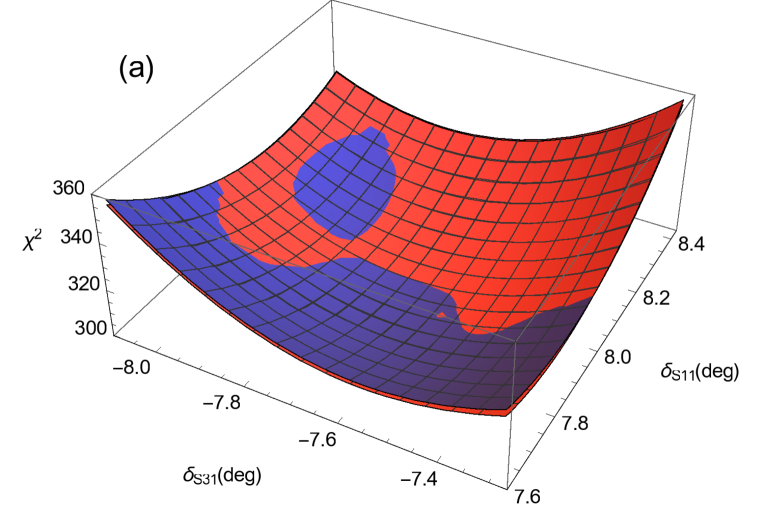
Starting from this last SE fit, and its best $\chi^{2}$, we see from Eq. (4) that the $\chi^{2}$ should increase quadratically as one moves away from the minimum. In the top panel of Fig. 1, we compare the $\chi^{2}$ variation for the two $S$-wave amplitudes as given by the corresponding error matrix and an actual fit to data (the other two partial waves are held at their best values $\hat{\delta}_{P11}$ and $\hat{\delta}_{P33}$). Shown is a region well beyond the $\Delta\chi^{2}=2.30$ ellipse that marks the 68% confidence region of a two-parameter fit (and well beyond the $\Delta\chi^{2}=4.72$ ellipse of a 4-parameter fit). The parabolic behavior of the correlated $\chi^{2}$ predicts well the actual $\chi^{2}$ within the shown region. Thus, the ${\cal O}({\bf A}^{3})$ corrections of Eq. (4) are indeed very small well beyond the region in which a fit can be considered good.

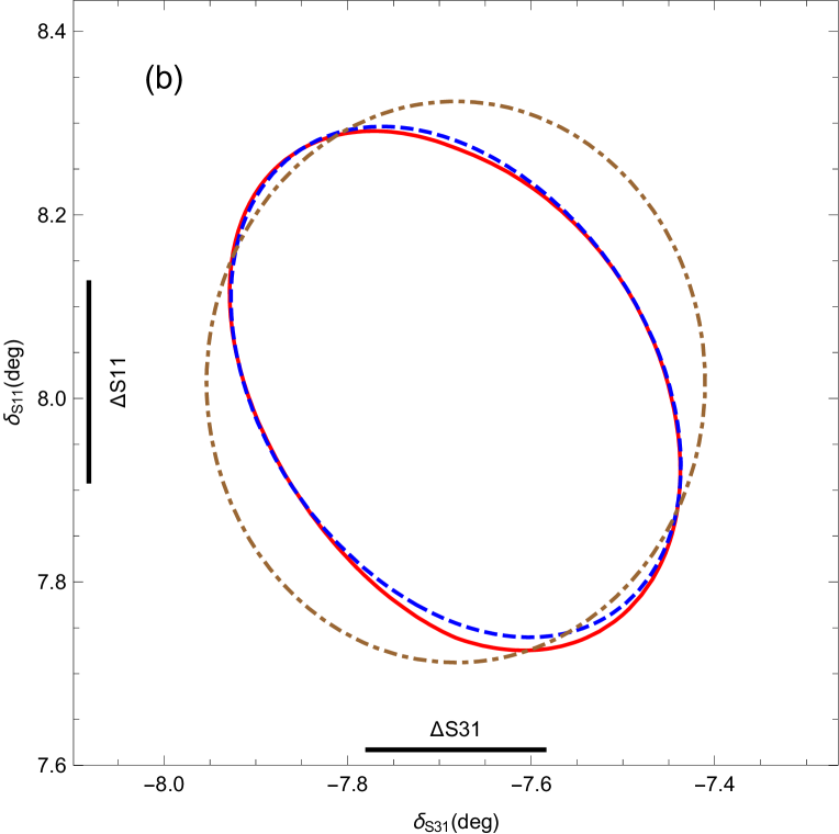
In the bottom panel of Fig. 1 we show the $\Delta\chi^{2}(\hat{\Sigma})=8$ ellipse from $\hat{\Sigma}$ (solid, red) and compare with the actual $\Delta\chi^{2}=8$ line (dashed, blue). The figure shows again that the covariance matrix predicts the rise of the $\chi^{2}$ well. For example, at $(\delta_{S11},\delta_{S31})=(8.42\,\text{deg},-7.28\,\text{deg})$ the difference between $\Delta\chi^{2}(\hat{\Sigma})$ and the actual $\Delta\chi^{2}$ is only 2, compared to an absolute scale given by $\chi^{2}=359$ at this point. Along the axes, the figure also shows the parameter errors, given by the maximal extensions of the $\Delta\chi^{2}=1$ ellipse.

In addition, a $\Delta\chi^{2}=8$ error ellipse is shown that is obtained from the covariance $\hat{\Sigma}_{0}$ in which all off-diagonal elements are set to zero, i.e., ignoring correlations (dash-dotted, brown). The effect is sizeable: At $(\delta_{S11},\delta_{S31})$ considered before one has $\Delta\chi^{2}(\hat{\Sigma})=56$ and $\Delta\chi^{2}(\hat{\Sigma}_{0})=31$, i.e., only $55\%$ of the correlated value. At higher energies, where parameters are generally more strongly correlated, this discrepancy becomes much larger.

The breakdown of $\chi^{2}$ contributions is then as follows: the $\chi^{2}$ at the minimum is $\chi^{2}(\hat{\bf A})$=301, the contribution from correlations amounts to $\Delta\chi^{2}=56$, and the sum $\chi^{2}=357$ is 0.5% different from the actual $\chi^{2}$ found from a comparison to data. In contrast, if one had mistakenly regarded the SE solutions as uncorrelated data points (as done in some analyses), a meaningless $\chi^{2}$=31 would have been obtained at $(\delta_{S11},\delta_{S31})=(8.42\,\text{deg},-7.28\,\text{deg})$.

To conclude this section, the effects of normalization are discussed. Recall that the minimum at ${\bf A}=\hat{\bf A}$ in the standard SE fit (third column of Table 1) is obtained allowing for renormalization of the minimizing function. The covariance matrix is then numerically estimated from the Hessian, $\hat{\Sigma}=2H^{-1}$ with $H_{ij}=\partial^{2}\chi^{2}/(\partial A_{i}\partial A_{j})$, using the penalized $\chi^{2}$ from Eq. (1), i.e., including the renormalization. To that end, the covariance matrix includes information about the change in normalization when moving away from the minimum, but with a value “frozen” at the minimum. Moving away from the minimum, both the fitted amplitudes and the fit function normalization factors work to reduce the $\chi^{2}$, resulting in a non-quadratic variation. However, if one is close to the minimum, the error matrix should still give a reasonable estimate of the data $\chi^{2}$.

Figure 2: The $\chi^{2}$ with renormalization. Notation as in Fig. 1. (a) The red (blue) surface shows the actual $\chi^{2}$ with renormalization (the $\chi^{2}$ predicted from the covariance matrix). (b) Contours of constant $\Delta\chi^{2}=8$ for the actual $\chi^{2}$ with renormalization (thick solid red), the $\chi^{2}$ predicted from the covariance matrix (thick dashed blue), and the case without renormalization from Fig. 1 (thin lines).

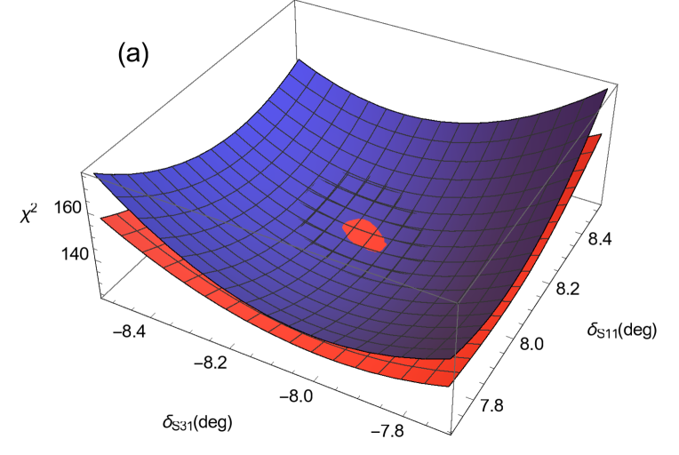
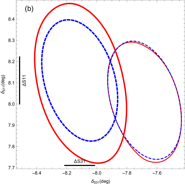
In Fig. 2, bottom panel, $\Delta\chi^{2}$ curves from the normalizable SE solution (thick) lines are shown. The curves from the previously discussed case (no normalization) are re-plotted for comparison (thin lines). The thick solid red (thick dashed blue) lines show the actual $\Delta\chi^{2}$ values (the $\Delta\chi^{2}$ values predicted from the covariance matrix). We observe larger deviations of the actual $\chi^{2}$ from the predicted one, that are a consequence of the discussed dynamic normalization, changing at any point in parameter space for the evaluation of the actual $\chi^{2}$. Note, however, that this example has been chosen for the $\Delta\chi^{2}=8$ contour, i.e., far away from the minimum. There, a maximal deviation of actual and predicted $\chi^{2}$ of 5 % is observed.

Figure 3: (a) Differential cross section at $T_{\pi}=91.7$ MeV and $\pi^{+}p$ data of Ref. dsg_data . (b) Polarization (P) at $T_{\pi}=87.2$ MeV and $\pi^{+}p$ data of Ref. p_data . The 90 MeV SE fit is shown; the normalization $N$ from Eq. (1) acquires a value of $N=0.98$ for the differential cross section (not applied in figure).

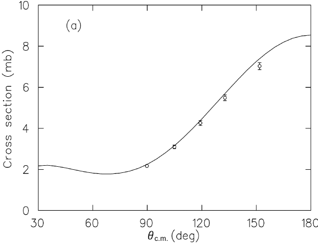
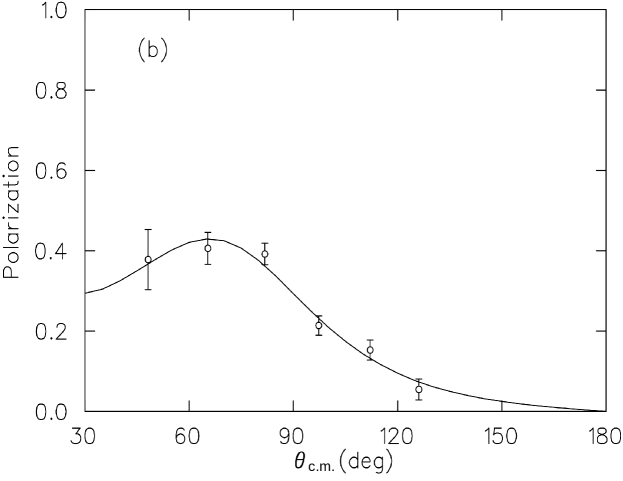
For further illustration, Fig. 3 shows a selection of data from the considered $T_{\pi}=87-92$ MeV energy bin and the SE fit obtained allowing normalization. The effect of normalization is visible for the differential cross section, which acquires a normalization factor of 0.98, constrained by the penalty term in Eq. (1). The factor, not applied in the figure, shifts the curve closer to the data, significantly reducing the $\chi^{2}$.

IV.1 Fits with fewer parameters

Some theory or model approaches describe fewer partial waves than provided in the covariance matrices. For example, chiral unitary approaches are often restricted to the lowest partial waves. How should one use the covariance matrices in these cases?

As an example, assume that model M describes $\delta_{S11}$, while the covariance matrix comprises $\delta_{S11}$ and $\delta_{S31}$ (see, e.g., the figures of this section). Suppose $\delta_{S11}$ in model M takes the value $\delta_{S11}=\hat{\delta}_{S11}+\Delta S11$. In the $\delta_{S11},\delta_{S31}$ space, this corresponds to the right vertical tangent to the $\Delta\chi^{2}=1$ ellipse. Then, there exists one value $\delta_{S31}$ such that indeed $\Delta\chi^{2}=1$. On the other hand, marginalizing the bivariate distribution over $\delta_{S31}$, one obtains a Normal distribution with variance $(\Delta S11)^{2}$, corresponding to a covariance matrix $\hat{\Sigma}=(\Delta S11)^{2}$. According to that reduced covariance matrix, the $\Delta\chi^{2}$ at $\delta_{S11}=\hat{\delta}_{S11}+\Delta S11$ has also increased by one, $\Delta\chi^{2}=1$. In summary, fitting the reduced covariance matrix is equivalent to fitting the entire covariance matrix, with $\delta_{S11}$ coming from model M, and optimizing all other parameters simultaneously. (Within M one cannot make any statement about the size of these other parameters/partial waves.)

The generalization to several parameters is straightforward. It can be shown that the reduced covariance matrix after marginalization is given by simply eliminating, from the full covariance matrix, the rows and columns corresponding to the marginalized parameters. Then, model M with fewer partial waves is fitted to that reduced matrix, and the unchanged $\chi^{2}(\hat{\bf A})$ is added according to Eq. (4).

V Summary and Conclusions

Covariance matrices and other fit properties of the SAID SE solutions are provided to allow other groups to carry out correlated $\chi^{2}$ fits to the elastic $\pi N$ scattering reaction. In principle, the obtained $\chi^{2}$ is then a good approximation to the $\chi^{2}$ one would obtain if fitting directly to experimental data. This has various practical advantages: Coulomb corrections are not an issue and normalization factors are included. However, the latter bear some subtleties as discussed. Furthermore, when fitting to SAID SE solutions, in the proposed manner, one implicitly accepts the chosen bin width and omission of non-linear contributions to the $\chi^{2}$ beyond the covariance matrix. In practice, we found these effects to be negligible, with the largest discrepancies coming from normalization. However, it has been checked that, close to the minimum, this effect is under control.

With correlated $\chi^{2}$ fits, it is now possible to fit the SAID SE solutions in a statistically meaningful way. For baryon spectroscopy, this is a prerequisite to quantify the significance of resonance signals, usually performed in multi-reaction fits in which, so far, the precise statistical impact of $\pi N$ partial waves has been unknown. Other approaches, such as quark-model calculations, CHPT, or unitary extensions thereof can also benefit from the proposed fitting scheme, allowing, e.g., for an improved determination of low-energy constants. The numerical input needed to carry out correlated $\chi^{2}$ fits is provided online.