Simulation of Stimulated Brillouin Scattering and Stimulated Raman Scattering In Shock Ignition

Abstract

We study stimulated Brillouin scattering (SBS) and stimulated Raman scattering (SRS) in shock ignition by comparing fluid and PIC simulations. Under typical parameters for the OMEGA experiments [Theobald et al., Phys. Plasmas 19, 102706 (2012)], a series of 1D fluid simulations with laser intensities ranging between 2$\times 10^{15}$ and 2$\times 10^{16}$ W/cm² finds that SBS is the dominant instability, which increases significantly with the incident intensity. Strong pump depletion caused by SBS and SRS limits the transmitted intensity at the 0.17$n_{c}$ to be less than 3.5$\times 10^{15}$ W/cm². The PIC simulations show similar physics but with higher saturation levels for SBS and SRS convective modes and stronger pump depletion due to higher seed levels for the electromagnetic fields in PIC codes. Plasma flow profiles are found to be important in proper modeling of SBS and limiting its reflectivity in both the fluid and PIC simulations.

I Introduction

Shock ignition (SI) Betti07 is a new high gain ignition scheme in inertial confinement fusion (ICF). The key process in SI is to generate a strong shock at the end of the compression stage by escalating the intensity of the incident laser to $10^{15}\sim 10^{16}$W/cm² Betti07 ; Perkins09 . In this high laser intensity regime, growth rates of many laser plasma instabilities (LPI) exceed their thresholds, such as the two plasmon decay (TPD), the stimulated Raman scattering (SRS), and the stimulated Brillouin scattering (SBS). Previous Particle-in-Cell (PIC) simulations showed large laser reflectivities at high intensities due to SBS and SRS Klimo10 ; Riconda11 , saturation of TPD due to plasma cavity formation Weber12 , intermittent LPI activities due to interplay of modes at different density regions Yan14 , and LPI’s dependence on plasma temperatures Weber15 . Both the integrated SI experiment on OMEGA Theobald12 and the PIC simulation Yan14 showed that the LPI generated hot electrons with a temperature of $\sim 30$ keV. A recent short pulse experiment found high level reflectivity of SBS under SI-relevant intensities Goyon13 . Due to the sensitivity and nonlinearity of LPI’s dependence on laser and plasma conditions, it is very important to explore the wide parameter space and understand the physics among the complicated LPI instabilities in SI.

In the low density region of the corona, SBS and SRS can be convective and their saturation levels depend on their seed levels as well as their convective gains. It is well known that in PIC codes high frequency modes of the electromagnetic fields have much higher noise levels than an actual plasma of the same physical conditionsokuda72 . How the inflated seed levels affect LPI in SI has not been studied so far. In addition the previous PIC simulations Klimo10 ; Riconda11 ; Weber12 ; Yan14 ; Weber15 did not include plasma flows, which can affect SBS reflectivity through the detuning of the ion acoustic wave resonance Galeev73 . In this paper, we study SBS and SRS for typical shock ignition conditions, including the flow velocity gradient, via a series of fluid and PIC simulations for the first time. Our fluid simulation results show that SBS is the dominant cause of the strong pump depletion for laser intensities of $I=2\times 10^{15}\sim 2\times 10^{16}$ W/cm ², and the flow velocity gradient has an important effect on limiting the SBS reflectivity. The transmitted laser intensity near the quarter critical region is limited to an asymptotic value of $I\sim 3.3\times 10^{15}$ W/cm ², which should be taken into account in SI design. The PIC simulations show similar physical trends as the fluid results but stronger pump depletion and higher saturation levels of SBS and SRS due to the higher numerical seed levels. The results here show the importance of incorporating realistic seed levels for correctly modeling LPI in the SI regime.

II The simulation results

Both the fluid and PIC simulations have been performed in one dimension (1D) to study SBS and SRS in the low density region before the quarter critical surface. They are complementary to the 2D simulations in Ref. Yan14 where the lowest density was $n=0.17n_{c}$ ($n_{c}$ is the critical density) and TPD was also studied. The PIC simulations are performed with OSIRIS Fonseca02 . The fluid simulations are performed with the HLIP code Hao14 , which is a 1D steady-state code solving the coexistent problem of SBS and SRS along the ray path, similar to DEPLETE Strozzi08 . The main equations in HLIP are listed as follows.

$$\frac{{\partial{I_{0}}}}{{\partial z}}=-\frac{{2{\nu_{0}}}}{{{v_{g0}}}}{I_{0}}-{\omega_{0}}{I_{0}}\sum\limits_{s=R,B}{\int{\frac{{({K_{s}}{Z_{s}}+{T_{s}})}}{{{\omega_{s}}}}d}{\omega_{s}}},$$ (1)

$$\frac{{\partial{Z_{s}}}}{{\partial z}}=\frac{{2{\nu_{s}}}}{{{v_{gs}}}}{Z_{s}}-{K_{s}}{I_{0}}{Z_{s}}-{I_{0}}{T_{s}},(s=R,B)$$ (2)

where $I$, $\omega$, $\nu$ and $v_{g}$ denote the laser intensity, the angular frequency, the collisional damping rate and the group velocity, respectively. The subscript $0$ refers to the incident light, and the subscript $s$ refers to the backscattered light from either SBS or SRS. Here, $Z_{s}$ denotes the intensity per angular frequency of the backscattered light with the integrated intensity ${I_{s}}(z)=\int{{Z_{s}}({\omega_{s}},z)d{\omega_{s}}}$. The seed term for the backscattered light $T_{s}$ is a calculated according to the Thomson scattering model Berger89 . The coupling coefficient

$${K_{s}}=\frac{{2\pi(k_{s}+k_{0})^{2}{e^{2}}}}{{{k_{s}}{k_{0}}{\omega_{0}}m_{e}^{2}{c^{4}}}}{\mathop{\rm Im}\nolimits}\left[\frac{\chi_{e}}{\varepsilon}(1+\sum\limits_{j}\chi_{j})\right],$$ (3)

is the local spatial growth rate of the backscattered light, where $k$ denotes the wavenumber of light, and as usual $e$, $m_{e}$, $c$ are the electron charge, the electron mass, and the speed of light in vacuum, respectively. The susceptibility for the electrons and the ion species $j$ are $\chi_{e}$ and $\chi_{j}$, respectively, and $\varepsilon=1+\chi_{e}+\sum_{j}\chi_{j}$ is the dielectric function, which depends on the frequency and wavenumber of the Langmuir wave or ion acoustic wave driven by the ponderomotive force. The kinetic term ${\rm Im}[\chi_{e}(1+\sum_{j}\chi_{j})/\varepsilon]$ is the ponderomotive response of the plasma to the light field Drake74 , which contains the effect of both Landau damping and phase detuning Strozzi08 .

Our simulation parameters are fitted from the LILAC Delettrez simulation results for the OMEGA integrated SI experiments Theobald12 . The incident laser has a wavelength of $\lambda_{0}=0.351\mu m$, and the length of the simulation box is $L=836\mu$m. In Fig. 1, the black solid line shows the density profile normalized by $n_{c}$ along the ray path . It is the same profile used in the 1D simulations in Ref. Yan14 and has a density scale length of $L_{n}=170\mu$m at the $1/4-n_{c}$ surface. The analytic expression of the normalized density is $n_{e}(x)=a_{6}x^{6}+a_{5}x^{5}+a_{4}x^{4}+a_{3}x^{3}+a_{2}x^{2}+a_{1}x+a_{0}$, where $x$ is the longitudinal distance from left boundary of simulation box in $\lambda_{0}$, $a_{6}=1.538\times 10^{-20},a_{5}=-8.225\times 10^{-17},a_{4}=1.797\times 10^{-13},a_{3}=-1.817\times 10^{-10},a_{2}=9.523\times 10^{-8},a_{1}=3.758\times 10^{-6}$, and $a_{0}=0.0156$. The density range is from $0.0156n_{c}$ to $0.4n_{c}$. The blue dashed line in Fig. 1 shows the plasma flow profile normalized by the vacuum speed of light $c$, in the form of $u(x)=-0.003567+1.494\times 10^{-6}x$. The ion components in the plasma are fully ionized C and H in 1:1 ratio. Two sets of the plasma temperatures are chosen from the LILAC simulations. In the low temperature (LT) case, $T_{e}=1.6$keV and $T_{C}=T_{H}=0.55$keV, which corresponds to the temperatures at the launch of the ignition pulse. In the high temperature (HT) case, $T_{e}=3.5$keV and $T_{C}=T_{H}=1.6$keV, which represents the temperatures at the peak intensity of the ignition pulse. A green dash-dot line is also drawn in Fig. 1 at the position of $n_{e}=0.17n_{c}$, where the transmitted laser intensity is diagnosed in this paper.

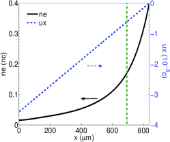
Figure 1: (Color online) The normalized density profile (black solid line) and plasma flow profile (blue dashed line) used in the simulations.

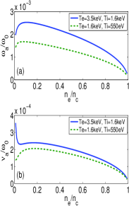
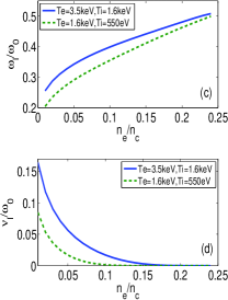
Figure 2: (Color online) The frequency (a) and the Landau damping rate (b) of the least-damped ion-acoustic waves; and the frequency (c) and the Landau damping rate (d) of the least-damped Langmuir waves in the CH plasma under two different temperatures.

For our CH plasma profile we have calculated the frequencies and Landau damping rates of the least-damped ion-acoustic waves and Langmuir waves for the two different temperature cases and the results are plotted in Fig. 2. These results are obtained by numerically solving the dispersion relation $\varepsilon(\omega,k)=0$ combined with the matching condition of the three-wave coupling $(\omega_{0}-\omega)^{2}-\omega_{pe}^{2}=(k-k_{0})^{2}c^{2}$. The results show the ion-acoustic waves correspond to the weakly damped slow ion-acoustic mode in Ref. vu94 . That for CH plasma the slow ion-acoustic mode is dominant is also consistent with the conclusion given by Williams et al. Williams95 . The results also show that the high temperature case has higher Landau damping rates for both the ion acoustic waves and the Langmuir waves.

II.1 The fluid simulation results

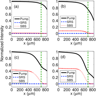
Figure 3: (Color online) Spatial profiles of the normalized intensities of the pump and backscattered light for the HT case (a,c) and the LT case (b,d), both with the plasma flow. The incident laser intensity is $I=2\times 10^{15}$W/cm² for (a,b) and $I=5\times 10^{15}$W/cm² for (c,d).

The fluid simulations for both the HT and LT cases have been performed with the same plasma flow profile and different laser intensities from $I=2\times 10^{15}$W/cm² up to $I=2\times 10^{16}$ W/cm ². The grid size is $\lambda_{0}$. Based on the frequency range of the weakest damped modes of ion-acoustic wave and Langmuir wave shown in Figs. 2(a) and 2(c), we set the wavelength of backscattered light of SRS from $400$nm to $715$nm, and the wavelength of backscattered light of SBS from $350.5$nm to $353$nm in HLIP to include the weakest damped modes on the ray path in our fluid simulations.

For each run, we can obtain the intensities of the pump laser and backscattered light along the ray path in the steady-state. Parts of the fluid simulation results are shown in Fig. 3, where the black solid line, the red dotted line, and the blue dashed line represent the intensity profiles of the pump laser, the SBS backscattered light, and the SRS backscattered light, respectively. All of the intensities are normalized by the incident laser intensity, which is $I=2\times 10^{15}$W/cm² in Figs. 3(a) and 3(b), and $I=5\times 10^{15}$W/cm² in Figs. 3(c) and 3(d). They show that SBS is the dominant instability, and the SBS reflectivity increases significantly as the incident laser intensity becomes higher. The SBS reflectivity is larger in the LT case than in the HT case, because Landau damping of the ion-acoustic wave is weaker in the LT case due to its larger $T_{e}/T_{i}\approx 2.9$ than the HT case where $T_{e}/T_{i}\approx 2.2$, as shown in Fig. 2.

In order to study the influence of the plasma flow on SBS, a set of simulations at $I=2\times 10^{15}$W/cm² have also been performed without the plasma flow, as shown in Figs. 4(a) and 4(b) for the HT and LT cases, respectively. Comparing them to Figs. 3(a) and 3(b), we can see that SBS is reduced by the plasma flow, resulting in lower SBS reflectivities. This is because the flow can Doppler shift the frequency of the local ion-acoustic wave and the gradient of the flow velocity can introduce phase mismatch between the SBS backscattered light wave coming from the higher density region and the local ion acoustic wave. This limits the further amplification of these convective modes at the lower density region Galeev73 .

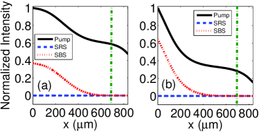
Figure 4: (Color online) Spatial profiles of the normalized intensities of the pump and backscattered light for (a) the HT case and (b) the LT case, without the consideration of the plasma flow $I=2\times 10^{15}$W/cm².

The SRS reflectivity maintains at a low level ($<1\%$) in Figs. 3 and 4. Indeed, no considerable SRS reflectivity is seen in the simulations until the laser intensity is higher than $1.5\times 10^{16}$W/cm². That is because the density scale length here, $L_{n}=170\mu$m, is small enough to detune the match condition between the local electronic plasma wave and the SRS backscattered wave from the higher density region. So the density gradient limits the SRS reflectivity effectively in the lower laser intensity cases Galeev73 .

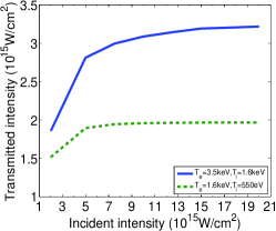
Figure 5: (Color online) The transmitted laser intensity at different incident laser intensity with the consideration of plasma flow.

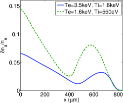
Figure 6: (Color online) Amplitudes of electron density perturbations due to SBS along the ray path.

The transmitted laser intensity at $n_{e}=0.17n_{c}$ for different incident laser intensity is shown in Fig. 5. It increases with the incident laser intensity but tends to an asymptotic maximum value, which is about 3.3$\times 10^{15}$ W/cm² for the HT case and 2$\times 10^{15}$ W/cm² for the LT case, due to larger reflectivity at high intensities. The transmitted intensity is always lower in the LT case than in the HT case, because Landau damping of the ion-acoustic wave and electronic plasma wave is lower in the LT case, resulting in stronger SBS and SRS activities. Although SBS is always the dominant instability in our fluid simulations, the SRS reflectivity is also considerable ($<10\%$) for the higher incident laser intensities. Fig. 6 shows the amplitudes of the electron density perturbations due to SBS at $I=5\times 10^{15}$W/cm² for both the HT and LT cases, showing $\delta n_{a}/n_{e}<0.15$, indicating nonlinear effects are not important here. For $I=2\times 10^{16}$W/cm² case, $\delta n_{a}<0.015n_{c}$ remains small even though $\delta n_{a}/n_{e}$ can be as large as 0.9 at left boundary due to very small $n_{e}$. Nonlinear effects at the high intensity may be important.

II.2 The PIC simulation results

The OSIRIS Fonseca02 simulations use the same plasma parameters as shown in Fig. 1, and laser intensities of $I=2,5,10\times 10^{15}$W/cm² for both the HT and LT cases. All the simulations use the 2nd-order spline current deposition scheme with current smoothing. The grid size is $\Delta x=0.1c/\omega_{0}$, and the time step is $\Delta t=0.0707/\omega_{0}$. The electron-ion collision is included in all PIC simulations by turning on the binary collision module in OSIRIS Yan12 . Boundary conditions are chosen to be open for the electromagnetic fields, and thermal bath for the particles Yan14 . The flow velocity profile is implemented by adding a flow velocity $u(x)$ to the thermal velocities of particles initially with $u(L)=0$ at the right boundary. At the left boundary $u(0)=-0.003567c$. The flow profile has the same velocity gradient as the LILAC simulation. The particles drift toward the left boundary and are re-injected into the simulation box with the initial temperature. The difference in the particle energy is recorded to diagnose the net energy flux of the particles leaving the simulation box.

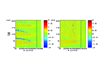
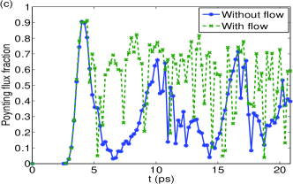
Figure 7: (Color online) Evolution of the normalized Poynting vectors for the HT case (a) without flow and (b) with flow, and (c) the time resolved Poynting flux fraction at $n_{e}=0.17n_{c}$. The incident laser intensity is $2\times 10^{15}$W/cm².

Fig. 7 shows the comparison of the PIC simulation results with and without the plasma flow velocity in the HT case with $I=2\times 10^{15}$W/cm². In Figs. 7(a) and 7(b), the longitudinal component of the Poynting vector, normalized by the incident Poynting vector at the left boundary, is shown. Stronger bursts of backscattered light are seen in the case without the plasma flow. This also indicates that the reflectivity is largely due to SBS since SRS is not sensitive to the plasma flow velocity. Correspondingly, the transmitted Poynting flux fraction at $n_{e}=0.17n_{c}$ shows that the pump depletion is also stronger when the plasma flow velocity is not considered, which is consistent with our fluid simulations.

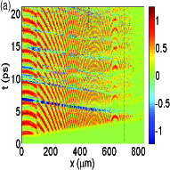
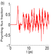
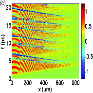
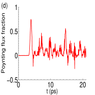
Figure 8: (Color online) Evolution of normalized Poynting vectors for (a) the HT case and (c) the LT case, and the time resolved Poynting flux fraction at $n_{e}=0.17n_{c}$ for (b) the HT case and (d) the LT case. The incident laser intensity is $5\times 10^{15}$W/cm² and the plasma flow is included.

Figs. 8(a) and 8(c) show the evolution of the Poynting vectors for the HT and LT cases respectively, when $I=5\times 10^{15}$W/cm² and with the plasma flow. To separate SBS and SRS reflectivities in the PIC simulations, we spatially Fourier-transform the $B_{z}$ field near the left boundary, and filter the data within the wavenumber region of SRS backscattered light in k-space to obtain the SRS reflectivity at every dumping step. The temporal average value for the total reflectivity can be obtained from the Poynting vector at left boundary. The SBS reflectivity is the difference of the two. We find a temporal average SBS reflectivity of approximately $31\%$ in the HT case and $51\%$ in the LT case, which indicates that SBS is also strong in the PIC simulations, especially for the LT case. The time resolved transmitted Poynting flux fraction at $n_{e}=0.17n_{c}$ is shown in Figs. 8(b) and 8(d). Its temporal average value is $20\%$ in the LT case, lower than the $32\%$ in the HT case. This indicates a significant SRS reflectivity, which is different from the fluid results.

Table 1: Simulated transmitted intensity fractions

Laser intensity	Temperature	Transmitted intensity fraction
(W/cm2)	conditions	HLIP	OSIRIS
$2\times 10^{15}$	HT case	$93\%$	$60\%$
	LT case	$76\%$	$25\%$
$5\times 10^{15}$	HT case	$56\%$	$32\%$
	LT case	$38\%$	$20\%$
$1\times 10^{16}$	HT case	$31\%$	$12\%$
	LT case	$20\%$	$8\%$

II.3 The seed level analysis

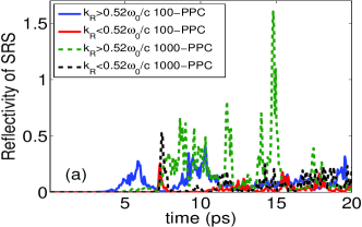
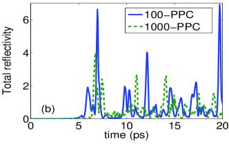
Figure 9: (Color online) Evolution of (a) SRS reflectivity and (b) total reflectiviy for the LT case. The incident laser intensity is $5\times 10^{15}$W/cm² and the plasma flow is included.

The larger reflectivities, especially the SRS reflectivities, in the OSIRIS simulations compared to the HLIP simulations can be attributed to many differences of the two codes. OSIRIS is fully kinetic and nonlinear while HLIP lacks both. However, even in the OSIRIS simulations, the dominant contribution to the SRS reflectivity comes from the convective modes in the low density region (see below). Therefore the seed levels for the convective SRS and SBS can be important to their saturation and the resultant reflectivities. To study the seed level effects, we repeat the LT case with $I=5\times 10^{15}$W/cm² and plasma flow, by using $1000$ particles per cell (PPC) for comparison. The results are compared with the 100-PPC case as shown in Figs. 9(a) and 9(b). For both cases, the SRS reflectivity is dominated by modes of $k>0.52\omega_{0}/c$, which are the convective modes in the region of $n<0.2n_{c}$ [Fig.9(a)]. The time-averaged total reflectivity drops from 64% (100-PPC) to 50% (1000-PPC) [Fig.9(b)]. This drop is mainly due to the drop of the SBS reflectivity, which changes from 51% (100-PPC) to 30% (1000-PPC). The SRS reflectivity increases from 13% (100-PPC) to 20% (1000-PPC) [Fig.9(a)], due to competition between SRS and SBS Berger98 ; Walsh84 ; Villeneuve87 . This also shows that in the OSIRIS simulations, SRS and SBS are probably in the nonlinear regime. In contrast, the level of SRS in the HLIP simulations is much smaller.

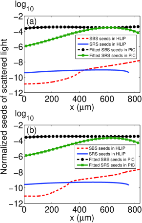
Figure 10: (Color online) The normalized seed level profiles of all SBS and SRS modes along the ray path for (a) the HT case and (b) the LT case when $I=5\times 10^{15}$W/cm². All of the intensities are normalized by $I$. The black dashed lines with sold circles show the SBS seeds and the green sold lines with crosses are the SRS seeds diagnosed in the OSIRIS simulations. The red dashed lines and blue solid lines are the integrated total seeds for the SBS and SRS backscattered light respectively given in HLIP based on the Thomson scattering model Hao14 .

To resolve the difference in reflectivity and pump depletion between the fluid and PIC simulations, we analyze the seed levels for the convective SBS and SRS in the two kinds of simulations. In order to diagnose the seed levels for the backscattered light in OSIRIS, the $B_{z}$ field data is dumped every $20$ calculation steps and divided into different windows in time and space. The time and spatial dimensions of each such window are $4000\Delta t$ and $5000\Delta x$. Through 2D Fourier transform of the data in the time-space window, signals of the backscattered light and incident light can be separated in the $\omega$-$k$ phase space. Summing up the signals of the backward light for SRS and SBS at different locations in the presence of the pump, we can obtain the seed levels defined in the same way as those used in HLIP.

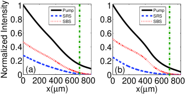
Figure 11: (Color online) Spatial profiles of normalized intensities of the pump and backscattered light for (a) the HT case and (b) the LT case when $I=5\times 10^{15}$W/cm², by using the seeds fitted from PIC simulations in HLIP code.

Figure 10 shows the seed levels in the two kinds of the simulations for the HT and LT cases when $I=5\times 10^{15}$W/cm². The seeds in the OSIRIS simulations are many orders of magnitudes larger than those calculated in HLIP. When HLIP uses the fitted seed profiles from OSIRIS instead of its own seed model, a significant growth of SRS can be obtained as shown in Fig. 11. The effect of a higher seed level on SBS is less significant, moderated by the pump depletions due to the inflated SRS. Overall, the new HLIP simulations show a higher pump depletion closer to the OSIRIS results. Other possible causes for difference exist between the two codes, such as re-scattering of SRS and generation of cavity Klimo10 (which is possible only at the inflated SRS level and not possible at the level shown in the fluid simulation with normal seed levels), kinetic and non-steady-state physics all in OSIRIS but not HLIP. Another possibility is the density-modulation-induced absolute SRS modes Nicholson76 , However, the different seed levels should be an important cause for the difference in pump depletion between the OSIRIS and HLIP simulation results.

III Discussion and Summary

A recent PIC study of the temperature effects on LPI in SI also found that the largest energy losses are due to the backscattering from SBS rather than SRS when $T_{e}\leq 5$keV and reflectivity of SBS decreases as $T_{e}$ increases Weber15 , even though those simulations were without flow and with a small scale length of 60 $\mu m$. In previous small-scale-length PIC simulations Riconda11 ; Weber15 ; Weber12 , pump depletion through convective SRS and SBS in the low density region was not significant, due to the small lengths. The long-scale-length simulations here show that the convective modes can lead to significant pump depletion before the quarter-critical surface and an accurate assessment of this requires control of the seed levels in simulations.

Neither of the two kinds of the simulations in the current work can fully match for the backscattering measured in the experimentTheobald12 . The overall pump reflectivities in the experiment were much lower than the OSIRIS results, likely due to the inflated seed levels. For the low intensities, the experiment showed a stronger SBS reflectivity than SRS, agreeing with the HLIP results. However, the experiments showed a rapidly increasing SRS reflectivity as the spike beam intensity increased, eventually exceeding the SBS reflectivity at $I=8\times 10^{15}$ W/cm². This is very different from the HLIP results. One possible source of this discrepancy is the hydro profile used in the simulations, which was taken from the LILAC simulation that had only the drive beams, not the spike beams. The profile may be significantly different from the actual one when the spike beams were on. Furthermore, the SRS gain model in HLIP does not include the possibility of absolute SRS and high-frequency hybrid modes afeyan97 in the quarter-critical region, which have been seen in previous 2D OSIRIS simulation in $n=0.17-0.33n_{c}$ with $I=2\times 10^{15}$ W/cm²Yan14 . The PIC simulations did show significant SRS reflectivity as the pump intensity increased. However, the inflated seed levels for the convective modes may have exaggerated the absolute levels.

In summary, SBS and SRS for typical laser and plasma conditions in shock ignition have been studied using the fluid and PIC simulations. Results show that SBS is the main cause for strong pump depletion, which limits the intensity of laser light arrived at the quarter critical density region. The plasma flow velocity gradient is shown to affect the SBS reflectivity. The seed level analysis also finds that the seed levels for both SRS and SBS in the PIC simulations are much higher than those in an actual plasma, which causes the stronger pump depletion in the PIC simulations. Comparison with the experiment shows the need of new simulation tools with both realistic seed levels and more comprehensive physics.

IV acknowledgments

The authors would like to acknowledge the OSIRIS Consortium for the use of OSIRIS. This work was supported by DOE under Grant No. DE-FC02-04ER54789 and DE-SC0012316; by NSF under Grant No. PHY-1314734; and by National Natural Science Foundation of China (NSFC) under Grant No. 11129503. The research used resources of the National Energy Research Scientific Computing Center. The support of DOE does not constitute an endorsement by DOE of the views expressed in this paper.

References

- (1) R. Betti, C. D. Zhou, K. S. Anderson, L. J. Perkins, W. Theobald, and A. A. Solodov, Phys. Rev. Lett. 98, 155001 (2007).
- (2) L. J. Perkins, R. Betti, K. N. LaFortune, and W. H. Williams, Phys. Rev. Lett. 103, 045004 (2009).
- (3) O. Klimo, S. Weber, V. T. Tikhonchuk, and J. Limpouch, Plasma Phys. Control. Fusion 52, 055013 (2010).
- (4) C. Riconda, S. Weber, V. T. Tikhonchuk, and A. Héron, Phys. Plasmas 18, 092701 (2011).
- (5) S. Weber, C. Riconda, O. Klimo, A. Héron, and V. T. Tikhonchuk, Phys. Rev. E 85, 016403 (2012).
- (6) R. Yan, J. Li, and C. Ren, Phys. Plasmas 21, 062705 (2014).
- (7) S. Weber and C. Riconda, High Power Laser Science and Engineering 3, e6 (2015).
- (8) W. Theobald, R. Nora, M. Lafon, A. Casner, X. Ribeyre, K. S. Anderson, R. Betti, J. A. Delettrez, J. A. Frenje, V. Y. Glebov, et al., Phys. Plasmas 19, 102706 (2012).
- (9) C. Goyon, S. Depierreux, V. Yahia, G. Loisel, C. Baccou, C. Courvoisier, N. G. Borisenko, A. Orekhov, O. Rosmej, and C. Labaune, Phys. Rev. Lett. 111, 235006 (2013).
- (10) H. Okuda, J. Comput. Phys. 10, 475 (1972).
- (11) A. A. Galeev, G. Laval, T. M. O’ Neil, M. N. Rosenbluth, and R. Z. Sagdeev, JETP Lett. 17, 85 (1973).
- (12) R. Fonseca, L. Silva, F. Tsung, V. Decyk, W. Lu, C. Ren, W. Mori, S. Deng, S. Lee, T. Katsouleas et al., Lect. Notes Comput. Sci. 2331, 342 (2002).
- (13) L. Hao, Y. Q. Zhao, D. Yang, Z. J. Liu, X. Y. Hu, C. Y. Zheng, S. Y. Zou, F. Wang, X. S. Peng, Z. C. Li, S. W. Li, T. Xu, and H. Y. Wei, Phys. Plasmas 21, 072705 (2014).
- (14) D. J. Strozzi, E. A. Williams, D. E. Hinkel, D. H. Froula, R. A. London, and D. A. Callahan, Phys. Plasmas 15, 102703 (2008).
- (15) R. L. Berger, E. A. Williams, and A. Simon, Phys. Fluids B 1, 414 (1989).
- (16) J. F. Drake, P. K. Kaw. Y. C. Lee, G. Schmidt, C. S. Liu, and M. N. Rosenbluth, Phys. Fluids 17, 778 (1974).
- (17) J. Delettrez and E. B. Goldman, Laboratory for laser energetics, University of Rochester, Rochester, NY, LLE Report No. 36, 1976.
- (18) H. X. Vu, J. M. Wallace, and B. Bezzerides, Phys. Plasmas 1, 3542 (1994).
- (19) E. A. Williams, R. L. Berger, R. P. Drake, A. M. Rubenchik, B. S. Bauer, D. D. Meyerhofer, A. C. Gaeris, and T. W. Johnston, Phys. Plasmas 2, 129 (1995).
- (20) R. Yan, C. Ren, J. Li, A. V. Maximov, W. B. Mori, Z. M. Sheng, and F. S. Tsung, Phys. Rev. Lett. 108, 175002 (2012).
- (21) R. Berger, C. Still, E. Williams, and A. Langdon, Phys. Plasmas 5, 4337 (1998).
- (22) C. J. Walsh, D. M. Villeneuve, H. A. Baldis, Phys. Rev. Lett. 53, 1445 (1984).
- (23) D. M. Villeneuve, H. A. Baldis, J. E. Bernard, Phys. Rev. Lett. 59, 1585 (1987).
- (24) D. R. Nicholson, Phys. Fluids 19, 889 (1976).
- (25) B. B. Afeyan and E. A. Williams, Phys. Plasmas 4, 3827 (1997).