Fluid of fused spheres as a model for protein solution

Abstract

In this work we examine thermodynamics of fluid with ‘‘molecules’’ represented by two fused hard spheres, decorated by the attractive square-well sites. Interactions between these sites are of short-range and cause association between the fused-sphere particles. The model can be used to study the non-spherical (or dimerized) proteins in solution. Thermodynamic quantities of the system are calculated using a modification of Wertheim’s thermodynamic perturbation theory and the results compared with new Monte Carlo simulations under isobaric-isothermal conditions. In particular, we are interested in the liquid-liquid phase separation in such systems. The model fluid serves to evaluate the effect of the shape of the molecules, changing from spherical to more elongated (two fused spheres) ones. The results indicate that the effect of the non-spherical shape is to reduce the critical density and temperature. This finding is consistent with experimental observations for the antibodies of non-spherical shape.

Key words: non-spherical proteins, liquid-liquid transition, directional forces, aggregation, thermodynamic perturbation theory

PACS: 87.15.A-, 87.15.ad, 87.15.km, 87.15.nr, 82.60.Lf, 64.70.Ja

Abstract

В цiй роботi ми дослiджуємо термодинамiку плину з ‘‘молекулами’’, представленими двома спаяними твердими сферами, якi декорованi вузлами з притягувальними потенцiалами типу квадратної ями. Взаємодiя мiж цими вузлами є короткодiюча i спричиняє асоцiацiю мiж частинками спаяних сфер. Модель може бути використана для дослiдження несферичних (чи димеризованих) протеїнiв у розчинi. Термодинамiчнi величини системи розраховуються за допомогою модифiкацiї термодинамiчної теорiї збурень Вертгайма, i результати порiвнюються з новими симуляцiями методом Монте Карло при iзобарично-iзотермiчних умовах. Зокрема, нас цiкавить фазове розшарування рiдина-рiдина в таких системах. Модельний плин використовується для оцiнки ефекту форми молекул, що змiнюється вiд сферичної до бiльш видовженої (двi спаянi сфери). Результати вказують, що ефект несферичної форми має зменшувати критичну густину i температуру. Це узгоджується з експериментальними спостереженнями для антитiл iз несферичною формою.

Ключовi слова: несферичнi протеїни, перехiд рiдина-рiдина, напрямляюча сила, агрегацiя, термодинамiчна теорiя збурень

1 Introduction

Aggregation of proteins in solution is both desired and undesired. It represents the first step in the downstream processing, i.e., salting out of the proteins for the purpose of cleaning and application. It is also one of the intermediate steps in the process of protein crystallization. The unwanted, pathological, protein aggregation is known to cause several diseases. Very importantly, bio-pharmaceutical drugs should be free of aggregates, otherwise they may be harmful. To increase the stability of protein in aqueous solutions is, therefore, an important technical problem. For an excellent review of the theoretical and experimental studies of protein solutions see reference [1].

The class of proteins we are interested in here are the so-called globular proteins. A typical representative of this class is lysozyme, which was extensively studied both experimentally and theoretically (see for example [1], Chapter 9). Despite their complicated 3D structure, many properties of protein solutions can be successfully described using relatively simple models [2, 3, 4, 5, 6, 7, 8]. Globular proteins are in their native form (we assume that during the experimental treatment they do not denature) most often pictured as perfectly spherical objects. This naïve representation is in reality never satisfied, it is used merely to simplify the calculations. There is a large list of non-spherical proteins, for example the shape of lysozyme mentioned above is ellipsoidal, including antibodies, lactoferrin, and others, where more complex geometry of particles would need to be taken into account to generate realistic results. This is important because the interactions leading to protein aggregation are directional and of short-range.

The shape of protein molecules influence their mutual interaction directly and indirectly. For example, (i) depletion interaction is largely dependent on the shape of particles [9]. (ii) Experimentally, it is observed that many of proteins with roughly spherical shape exhibit upper critical solution temperature at protein concentration equal to 240 g/L [1, 10, 11]. In contrast to that, Y-shaped antibodies exhibit the shift toward much lower values, way down to 100 g/L [12, 13]. (iii) The hydrodynamic radii of the non-spherical objects are different, therefore, their hydrodynamic and transport coefficients [14], as well as, kinetic parameters [15] are modified. It is also known that classical nucleation theory has difficulties in describing the crystallization of other than spherical (for example ellipsoidal) particles [1, 16].

Recently, we used a simple spherical model [8] to analyze experimental results for the cloud-point temperatures in aqueous protein solutions with added salts [10, 11]. We modelled the solution as a one-component system; the protein molecules were represented as perfect spheres, embedded in the continuum solvent composed of water, buffer, and various simple salts. The attractive short-range interactions between the proteins were due to the square-well sites located on the surface of protein molecules. The model was numerically evaluated using Wertheim’s perturbation theory [17, 18, 19]. The short-range and directional nature of the interactions among proteins led to good agreement with the experimental data for the liquid-liquid phase diagram in case of lysozyme and $\gamma$-crystallin solutions [10, 11]. With knowledge of the experimental cloud-point temperature as a function of composition of electrolyte present in the system, the model gave predictions for the liquid-liquid coexistence curves, the second virial coefficients, and other similar properties under such experimental conditions.

One weakness of the model presented above was its simplified geometry. Neither lysozyme nor other proteins are spherical, and some of them for example, lactoferrin [20] look more like two fused spheres. The other weakness was that we assume for protein molecules to exist in form of monomers, which is not true. Even in very dilute solutions, proteins can be at least partially dimerized. The purpose of the present work is to investigate how the relaxing of these two basic assumptions influence the liquid-liquid coexistence curve.

The models for the association of spherically symmetric particles into dimer molecules are of considerable interest to science and technology and have been actively studied earlier. Of particular interest for us are the models where there is an inter-penetration (‘‘fusing’’ of cores) of the spherical particles upon association so that the bonding length $L$ is less than the core diameter $\sigma$. The ‘‘shielded sticky shell’’ and the ‘‘shielded sticky point’’ models of Stell and co-workers [21, 22, 23] and their extensions [24, 25, 26], belong to this group of models and are the starting point for our work. These types of the models were studied using regular [21, 22, 24] and multi-density [27, 28, 29, 23, 25, 26] integral equation theories.

In the present study, we use spherical particles as building blocks, which are fused together to form a new species. In this way, we compose the molecule with arbitrary spacing $L$ between the centers of spheres. Next, we decorate the surfaces of fused-sphere molecules with the attractive short-range binding sites, which may cause the association of the newly formed molecules. Such an extension of the protein model follows from our previous work [8]. Here, we wish to explore the effects of the non-spherical shape on various thermodynamic properties.

Different versions of the model of dimerizing particles, represented by the tangentially bonded chain molecules, have been studied earlier [30, 31]. In this type of the model, dimerization occurs due to square-well bonding site, placed on the surface of one of the hard-sphere terminal monomer of each chain. Theoretical description of the model was carried out using first order thermodynamic perturbation theory (TPT1) of Wertheim [17, 18]. There are two major features of our model that set it apart from the models studied earlier, i.e., (i) in our model the molecules are represented by the two hard-sphere monomers fused at a distance $L$, which is less than the contact distance $\sigma$ and (ii) the molecules upon association can form a three-dimensional network. Due to the former feature of the model, a straightforward application of Wertheim’s multi-density approach fails to produce accurate results [29, 32, 33]. In the present work, we use a modified version of the TPT1, which takes into account the change of the overall packing fraction of the system due to the association forces [29, 34, 35]. The accuracy of our modified TPT1 approach is checked by the newly generated Monte Carlo simulation data.

2 Model, theory, and simulations

2.1 Model

We introduce a one component model of spherical particles, decorated with additional binding sites of two different types, A and B. The binding site A is placed within the sphere, with the displacement $d_{\textrm{A}}\leqslant\sigma/2$, while an arbitrary number $K_{\textrm{B}}$ of binding sites of type B is located on the surface of the sphere (the displacement $d_{\textrm{B}}=\sigma/2$). The model is visualized in figure 1. We consider a special case, where we exclude the cross interactions among sites A and B. The total pair potential is written as follows:

$$u(\mathbf{{r}}) = u_{\mathrm{R}}(r)+\sum_{M=\textrm{A}}^{\textrm{B}}u_{{MM}}(\mathbf{{x}}_{{MM}}),$$ (2.1)

where $u_{\mathrm{R}}$ is the pair potential for hard spheres, and $u_{\textrm{AA}}$ and $u_{\textrm{BB}}$ are inter-particle site-site potentials. The vector $\mathbf{{r}}$ ($r=|\mathbf{{r}}|$) connects the centers of hard spheres, and $\mathbf{{x}}_{{MM}}$ denotes the inter-particle vector connecting two sites of the type $M$. As mentioned above, $u_{{MM}}$ is the orientation dependent square-well potential between the sites $M\in\{\text{A,B}\}$, defined as follows:

$$u_{MM}(\mathbf{{x}}_{MM}) = \left\{\begin{array}[]{ll}\varepsilon^{\prime}_{MM}=-\varepsilon_{MM}-\xi_{MM},&\quad\text{for}\quad|\mathbf{{x}}_{MM}|<a_{MM},\\ 0,&\quad\text{for}\quad|\mathbf{{x}}_{MM}|\geqslant a_{MM}.\end{array}\right.$$ (2.4)

The site A causes inter-penetration of particles (see figure 3). Note that we need the term $\xi_{\textrm{AA}}\rightarrow\infty$ to compensate for the hard sphere repulsion. For the periphery sites B, we do not need such a term, therefore $\xi_{\textrm{BB}}\rightarrow 0$. To fuse hard cores at separation $L$, we choose $d_{\textrm{A}}=L/2$ and take the limit $\varepsilon_{\textrm{AA}}\rightarrow\infty$.

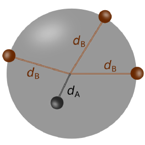
Figure 1: (Color online). Spherical particles with diameter $\sigma$ are capable of, due to the attraction among sites of type A, penetrating to form fused sphere molecules. The cross interactions A–B are prohibited. In this figure, $K_{\textrm{B}}=3$.

2.2 Theory

An appropriate theoretical approach to be used is the first-order Wertheim’s thermodynamic perturbation theory (TPT1) [17, 18]. According to this theory, the Helmholtz free energy of the system can be written as a sum of several terms:

$$A = A^{\textrm{id}}+A^{\textrm{hs}}+A^{\textrm{A--A}}+A^{\textrm{B--B}},$$ (2.5)

where $A^{\textrm{id}}+A^{\textrm{hs}}=A_{\textrm{R}}$ is the free energy of the reference system represented by the hard-sphere system [36] and $A^{\textrm{A--A}}+A^{\textrm{B--B}}=A^{\textrm{ass}}$ is the contribution due to A–A and B–B interactions. Following Chapman et al. [19], we have:

$$\frac{\beta(A-A_{\textrm{R}})}{N} = \frac{\beta A^{\textrm{A--A}}}{N}+\frac{\beta A^{\textrm{B--B}}}{N},$$ (2.6)

$$\frac{\beta A^{\textrm{A--A}}}{N} = \ln{X_{\mathrm{A}}}-\frac{1}{2}X_{\mathrm{A}}+\frac{1}{2},$$ (2.7)

$$\frac{\beta A^{\textrm{B--B}}}{N} = K_{\textrm{B}}\left(\ln{X_{\mathrm{B}}}-\frac{1}{2}X_{\mathrm{B}}+\frac{1}{2}\right).$$ (2.8)

Here, $\beta=(k_{\textrm{B}}T)^{-1}$ and $k_{\textrm{B}}$ is Boltzmann’s constant as usual, $T$ is the absolute temperature, and $N$ is the number of spheres. Further, $X_{M}$ defines the average number fraction of particles, which are not bonded through the binding site $M$. Parameters $X_{\textrm{A}}$ and $X_{\textrm{B}}$ are determined by the mass-action law [19]

$$X_{\textrm{A}} = \frac{1}{1+\rho\big{(}X_{\textrm{A}}\Delta_{\mathrm{AA}}+K_{\textrm{B}}X_{\textrm{B}}\Delta_{\mathrm{AB}}\big{)}},$$ (2.9)

$$X_{\textrm{B}} = \frac{1}{1+\rho\big{(}X_{\textrm{A}}\Delta_{\mathrm{BA}}+K_{\textrm{B}}X_{\textrm{B}}\Delta_{\mathrm{BB}}\big{)}},$$ (2.10)

where $\rho=N/V$ is the number density of spheres and $\Delta_{MN}$ connects the pair distribution function of hard spheres $g^{\mathrm{hs}}(r)$ (reference system) and the binding potential for sites $M$ and $N$. The corresponding $\Delta_{MN}$ parameters are:

$$\Delta_{{MN}} = 4\pi\int_{d_{M}+d_{N}}^{d_{M}+d_{N}+a_{MN}}g^{\mathrm{hs}}(r)\bar{f}_{{MN}}(r)r^{2}\mathrm{d}r\qquad\forall\;{M,N}\in\{\text{A,B}\}.$$ (2.11)

Expression for the solid-angle averaged Mayer function

$$\bar{f}_{{MN}}(r)=\int\int f_{{MN}}\big{(}\mathbf{{x}}_{{MN}}(\mathbf{{r}})\big{)}\mathrm{d}\Omega_{M}\mathrm{d}\Omega_{N}$$ (2.12)

was initially derived by Wertheim [37] and further generalized here to be

$$\bar{f}_{{MN}}(r) = \frac{\exp{\left(-\beta\varepsilon^{\prime}_{MM}\right)}-1}{24d_{M}d_{N}r}(a_{MN}+d_{M}+d_{N}-r)^{2}(2a_{MN}-d_{M}-d_{N}+r).$$ (2.13)

To suppress the cross interactions A–B, we set $\Delta_{\mathrm{AB}}=\Delta_{\mathrm{BA}}=0$, which finally yields two independent equations, written in a quadratic form

$$\rho\Delta_{\mathrm{AA}}X_{\textrm{A}}^{2}+X_{\textrm{A}}-1 = 0,$$ (2.14)

$$\rho K_{\textrm{B}}\Delta_{\mathrm{BB}}X_{\textrm{B}}^{2}+X_{\textrm{B}}-1 = 0.$$ (2.15)

2.2.1 Association parameters $\Delta_{\textrm{AA}}$ and $\Delta_{\textrm{BB}}$

The association parameter $\Delta_{\mathrm{AA}}$ is related to $X_{\textrm{A}}$ via equation (2.14) and to the free energy contribution due to A–A binding, by equation (2.7). For the complete association limit, i.e., fusing of hard cores at separation $L$, no monomer spheres are present, so $X_{\textrm{A}}=0$. We re-write the association parameter $\Delta_{\mathrm{AA}}$ and introduce the cavity correlation function $y^{\mathrm{hs}}(r)$ to obtain

$$\Delta_{\mathrm{AA}} = 4\pi\int_{2d_{\textrm{A}}}^{2d_{\textrm{A}}+a_{\textrm{AA}}}y^{\mathrm{hs}}(r)e^{\mathrm{hs}}(r)\bar{f}_{\mathrm{AA}}(r)r^{2}\mathrm{d}r,$$ (2.16)

where $e^{\mathrm{hs}}(r)=\exp[-\beta u_{\mathrm{R}}(r)]$. Note that, as already mentioned before, $2d_{\textrm{A}}=L$. By applying the sticky limit approximation [37], that is by assuming the constant value of $y^{\mathrm{hs}}$ within the integration domain, we obtain

$$\Delta_{\mathrm{AA}} = y^{\mathrm{hs}}(r=2d_{\textrm{A}})I_{\textrm{AA}},$$ (2.17)

$$I_{\textrm{AA}} = 4\pi\int_{2d_{\textrm{A}}}^{2d_{\textrm{A}}+a_{\textrm{AA}}}e^{\mathrm{hs}}(r)\bar{f}_{\mathrm{AA}}(r)r^{2}\mathrm{d}r.$$ (2.18)

The integral given by equation (2.18) is not used in further calculations and, accordingly, it will not be considered in more detail here.

Parameter $\Delta_{\textrm{BB}}$ determines the degree of association of fused spheres and the free energy contribution due to the B–B binding, see equations (2.8) and (2.15). Notice that due to the association between $A$-type of the sites, the packing fraction of fused spheres $\eta_{\textrm{eff}}$ is different from the packing fraction originally present (un-fused) hard spheres $\eta$. These fractions are related as follows:

$$\eta_{\textrm{eff}} = D(l^{*})\eta,$$ (2.19)

$$D(l^{*}) = \frac{1}{2}\bigg{(}{1+\frac{3}{2}l^{*}-\frac{1}{2}{l^{*}}^{3}}\bigg{)},$$ (2.20)

where $\eta=\pi\rho\sigma^{3}/6$ is the packing fraction of hard spheres and $l^{*}=L/\sigma$ is reduced A–A bonding distance. Using the sticky limit approximation [37] for $\Delta_{\mathrm{BB}}$ [equation (2.11)], we have:

$$\Delta_{\mathrm{BB}} = g^{\mathrm{hs}}(r=\sigma,\eta=\eta_{\textrm{eff}})I_{\textrm{BB}},$$ (2.21)

$$I_{\textrm{BB}} = 4\pi\int_{\sigma}^{\sigma+a_{\textrm{BB}}}\bar{f}_{\mathrm{BB}}(r)r^{2}\mathrm{d}r.$$ (2.22)

The integral in $I_{\textrm{BB}}$ can be evaluated analytically. We have used the Carnahan-Starling approximation for the contact value of $g^{\mathrm{hs}}$ at the effective packing fraction of fused spheres $\eta_{\textrm{eff}}$

$$g^{\mathrm{hs}}(r=\sigma,\eta=\eta_{\textrm{eff}})=\frac{2-\eta_{\textrm{eff}}}{2(1-\eta_{\textrm{eff}})^{3}}.$$ (2.23)

2.2.2 Cavity correlation function $y^{\mathrm{hs}}$

The last unknown quantity in equation (2.17) is the cavity correlation function of hard sphere fluid, $y^{\mathrm{hs}}$. It is calculated by using the Tildesley-Streett expression for pressure of the hard dumbbell fluid [38]. By choosing $K_{\textrm{B}}=0$, $d_{\textrm{A}}\leqslant\sigma/2$ and applying sticky limit conditions, i.e., $\varepsilon_{\mathrm{AA}}\rightarrow\infty$, $a_{\mathrm{AA}}\rightarrow 0$ while keeping the integral in equation (2.16) finite, our model reduces to the hard dumbbell fluid. We modify the mass action law [equation (2.14)], by inserting equation (2.17) with $X_{\textrm{A}}=\rho_{0}/\rho$, where $\rho_{0}$ stands for the number density of spheres, not bonded through binding site A (monomers). The result represents a different form of equation (110) of Wertheim’s paper [37]

$$\rho=\rho_{0}+\rho_{0}^{2}I_{\textrm{AA}}y^{\mathrm{hs}}(r=L).$$ (2.24)

Following Wertheim [37], we get the expression for the excess pressure in the form:

$$\beta(P-P_{\mathrm{R}})=-\frac{1}{2}(\rho-\rho_{0})\bigg{\{}1+\rho\frac{\partial\ln[y^{\mathrm{hs}}(r=L)]}{\partial\rho}\bigg{\}}.$$ (2.25)

We are now in position to obtain the cavity correlation function $y^{\mathrm{hs}}$ of hard sphere system. We use the Carnahan-Starling equation of state [36] for the reference system ($P_{\mathrm{R}}$) and the Tildesley-Streett equation of state [38] for the perturbed hard dumbbell system ($P$).

• Carnahan-Starling EOS:

  $$\frac{\beta P_{\text{R}}}{\rho} = \frac{1+\eta+\eta^{2}-\eta^{3}}{(1-\eta)^{3}}.$$ (2.26)

• Tildesley-Streett EOS:

  $$\frac{\beta P}{\rho_{\mathrm{d}}} = \!\frac{1\!+\!(1\!+\!Ul^{*}\!+\!V{l^{*}}^{3})\eta_{\mathrm{eff}}\!+\!(1\!+\!Wl^{*}\!+\!X{l^{*}}^{3})\eta_{\mathrm{eff}}^{2}\!-\!(1\!+\!Yl^{*}\!+\!Z{l^{*}}^{3})\eta_{\mathrm{eff}}^{3}}{(1\!-\!\eta_{\mathrm{eff}})^{3}},$$ (2.27)

where $\rho_{\mathrm{d}}=\rho/2$ is the number density of hard dumbbells. The set of numerical parameters $U$, $V$, $W$, $X$, $Y$, $Z$ is given in table 1.

Table 1: Parameters in the Tildesley-Streett EOS [38].

$U$	$V$	$W$	$X$	$Y$	$Z$
0.37836	1.07860	1.30376	1.80010	2.39803	0.35700

Within the framework of Wertheim’s theory, we must set $\rho_{0}=0$ in equation (2.25) to recover the fluid of hard dumbbell particles (no monomers present). Next, we use equations (2.19), (2.20), (2.25) and equations of state [(2.26) and (2.27)] to obtain the derivative

$$\rho\frac{\partial\ln[y^{\mathrm{hs}}(r=L)]}{\partial\rho} = -\frac{\sum_{i=1}^{6}a_{i}\eta^{i}}{1+\sum_{i=1}^{6}b_{i}\eta^{i}}.$$ (2.28)

The set of equations which determine $a_{i}$ and $b_{i}$ [$D\equiv D(l^{*})$] are as follows:

$$A = (1+Ul^{*}+V{l^{*}}^{3})D,$$ (2.29)

$$B = (1+Wl^{*}+X{l^{*}}^{3})D^{2},$$ (2.30)

$$C = (1+Yl^{*}+Z{l^{*}}^{3})D^{3},$$ (2.31)

with the arrays

$a_{1}=A+3D-8,$	$b_{1}=-3(1+D),$
$a_{2}=-3A+B+15D-3D^{2}+4,$	$b_{2}=3(1+3D+D^{2}),$
$a_{3}=3A-3B-C-3D-15D^{2}+D^{3},$	$b_{3}=-(1+9D+9D^{2}+D^{3}),$
$a_{4}=-A+3B+3C-3D+3D^{2}+5D^{3},$	$b_{4}=a_{2}D,$
$a_{5}=-B-3C+3D^{2}-D^{3},$	$b_{5}=a_{1}D^{2},$
$a_{6}=C-D^{3},$	$b_{6}=D^{3}.$

It is obvious $\rho\,\partial\ln[y^{\mathrm{hs}}(r=L)]/\partial\rho=\eta\,\partial\ln[y^{\mathrm{hs}}(r=L)]/\partial\eta$, therefore equation (2.28) can be easily integrated to yield:

$$\ln[y^{\mathrm{hs}}(r=L)] = -\int_{0}^{\eta}\frac{\sum_{i=1}^{6}a_{i}t^{i-1}}{1+\sum_{i=1}^{6}b_{i}t^{i}}\mathrm{d}t.$$ (2.32)

The integral was checked to be non-singular for all investigated $\eta$ and $l^{*}$ values. Numerical results for $\ln[y^{\mathrm{hs}}(r)]$ are for a few fluid densities shown in figure 2.

Figure 2: Logarithm of the cavity distribution function $y^{\mathrm{hs}}$ of hard spheres for $\rho\sigma^{3}$ is equal to: 0.4 (dashed line), 0.6 (dashed-dotted line) and 0.8 (solid line). The limit of $y^{\mathrm{hs}}$, $\lim_{r\rightarrow\sigma}y^{\mathrm{hs}}(r)$, coincides with equation (2.23) for the ‘‘non-effective’’ packing fractions $\eta$.

2.2.3 Other thermodynamic properties

Next, we calculate the excess pressure $P^{\textrm{ass}}=P-P_{\textrm{R}}$ and the excess chemical potential $\mu^{\textrm{ass}}=\mu-\mu_{\textrm{R}}$ needed in phase diagram calculations as also excess internal energy $E^{\textrm{ass}}=E-E_{\textrm{R}}$, due to association. Starting with the pressure, we have

$$\beta(P-P_{\textrm{R}})=\rho^{2}\frac{\partial\big{[}\beta(A-A_{\textrm{R}})/N\big{]}}{\partial\rho}=\rho\sum_{\textrm{M=A}}^{\textrm{B}}\bigg{(}\frac{\partial\big{[}\beta(A-A_{\textrm{ R}})/N\big{]}}{\partial X_{M}}\bigg{)}\bigg{(}\eta\frac{\partial X_{M}}{\partial\eta}\bigg{)}.$$ (2.33)

By inserting the appropriate derivatives from equations (2.6), (2.14), and (2.15), we get the final expression for the excess pressure. The second term $B$ is evaluated at $\eta_{\textrm{eff}}$, see equation (2.23), therefore upon differentiation we get an additional factor $D(l^{*})$

$$\beta(P-P_{\textrm{R}}) = \beta P^{\mathrm{AA}}+\beta P^{\mathrm{BB}},$$ (2.34)

$$\beta P^{\mathrm{AA}} = -\frac{\rho}{2}(1-X_{\textrm{A}})\left\{1+\eta\frac{\partial\ln[y^{\mathrm{hs}}(r=L)]}{\partial\eta}\right\},$$ (2.35)

$$\beta P^{\mathrm{BB}} = -\frac{\rho}{2}K_{\textrm{B}}(1-X_{\textrm{B}})\left\{1+D(l^{*})\eta\frac{\partial\ln[g^{\mathrm{hs}}(r=\sigma)]}{\partial\eta}\bigg{|}_{\begin{subarray}{c}\eta=\eta_{\textrm{eff}}\end{subarray}}\right\}.$$ (2.36)

The expression $\eta\partial\ln[y^{\mathrm{hs}}(r=L)]/\partial\eta$ is obtained from equation (2.28), while the second derivative $\partial\ln[g^{\mathrm{hs}}(r=L)]/\partial\eta\big{|}_{\begin{subarray}{c}\eta=\eta_{\textrm{eff}}\end{subarray}}$ is obtained analytically at $\eta=\eta_{\textrm{eff}}$ from equation (2.23)

$$\frac{\partial\ln[g^{\mathrm{hs}}(r=L)]}{\partial\eta}\bigg{|}_{\begin{subarray}{c}\eta=\eta_{\textrm{eff}}\end{subarray}} = \frac{5-2\eta_{\textrm{eff}}}{(1-\eta_{\textrm{eff}})(2-\eta_{\textrm{eff}})}.$$ (2.37)

The excess chemical potential $\mu^{\textrm{ass}}=\mu-\mu_{\textrm{R}}$ is obtained through the relation

$$\mu^{\textrm{ass}} = \frac{A^{\textrm{ass}}}{N}+\frac{P^{\textrm{ass}}}{\rho}.$$ (2.38)

The logarithmic term $\ln X_{\textrm{A}}$ in equation (2.7) is divergent for the complete association limit ($\Delta_{\mathrm{AA}}\gg 1$), therefore we re-write this term by using equation (2.17) as follows:

$$\ln X_{\textrm{A}}=\ln\bigg{(}\frac{-1+\sqrt{1+4\rho\Delta_{\mathrm{AA}}}}{2\rho\Delta_{\mathrm{AA}}}\bigg{)}{\approx}\ln\bigg{(}\frac{\sqrt{4\rho\Delta_{\mathrm{AA}}}}{2\rho\Delta_{\mathrm{AA}}}\bigg{)}=-\frac{1}{2}\ln[\rho y^{\textrm{hs}}(L)]-\frac{1}{2}\ln[I_{\textrm{AA}}(\beta)].$$ (2.39)

The second term in equation (2.39) is independent of density and, accordingly, does not contribute to the pressure. The expression for $P$ is the same as derived before [equations (2.34)–(2.36)]. The equilibrium conditions require the equality of chemical potential at a constant temperature (see equations below), so the second term in equation (2.39) cannot affect the coexistence curve. The equilibrium conditions read:

$$\mu(\rho_{\textrm{I}},T) = \mu(\rho_{\textrm{II}},T),$$ (2.40)

$$P(\rho_{\textrm{I}},T) = P(\rho_{\textrm{II}},T),$$ (2.41)

where $\rho_{\textrm{I}}$ and $\rho_{\textrm{II}}$ are the two coexisting densities. At this step, the phase diagram can be constructed by applying equations (2.40)–(2.41) as it is in more detail explained in the previous work [8].

Another thermodynamic quantity is the excess internal energy $E^{\textrm{ass}}=E-E_{\textrm{R}}$, obtained as

$$\frac{E-E_{\textrm{R}}}{N} = \frac{\partial\big{[}\beta(A-A_{\textrm{R}})/N\big{]}}{\partial\beta}=\frac{E^{\textrm{A--A}}}{N}+\frac{E^{\textrm{B--B}}}{N},$$ (2.42)

$$\frac{E^{\textrm{A--A}}}{N} = -\frac{\rho}{2}X_{\textrm{A}}^{2}\frac{\partial\Delta_{\textrm{AA}}}{\partial\beta},$$ (2.43)

$$\frac{E^{\textrm{B--B}}}{N} = -\frac{\rho}{2}(K_{\textrm{B}}X_{\textrm{B}})^{2}\frac{\partial\Delta_{\textrm{BB}}}{\partial\beta}.$$ (2.44)

Since ${E^{\textrm{A--A}}}/{N}$ is divergent, the only relevant part is ${E^{\textrm{B--B}}}/{N}$. Derivative $\partial\Delta_{\textrm{BB}}/\partial\beta$ is obtained analytically from equations (2.21)–(2.22), since $g^{\mathrm{hs}}$ is $\beta$ independent. Thermodynamic functions for the reference system of hard spheres, $\beta A_{\textrm{R}}/N$, $\beta P_{\textrm{R}}$, $u_{\textrm{R}}$ and $E_{\textrm{R}}/N$, can be found elsewhere [36].

2.3 $N,P,T$ Monte Carlo simulation

To validate the accuracy of the modified TPT1 approach, we performed Monte Carlo computer simulations in the $N,P,T$ ensemble [39]. We assumed fused spheres with one and two binding sites on each sphere, where the prescribed arrangement of sites was preserved during the simulation. Simulated molecules are schematically shown in figure 3. We adopted the sampling method suggested by Tildesley and Streett [40], where a single displacement parameter was needed to describe the translation and rotation of fused spheres. The simulation box contained 250 fused spheres (molecules), which is equivalent to 500 penetrating (original, un-fused) spheres. We defined the cycle with 250 attempts to move the object and by 1 attempt to change the volume box. Next, we defined the block to be equal to $5\times 10^{4}$ cycles. Initially, we performed 1 block, to equilibrate the system, while 4 independent blocks were needed to calculate thermodynamic properties via the block averaging. Simulations were performed for three $l^{*}$ values: 0.2, 0.6, 1.0, and four different pressures $Pk_{\text{B}}T/\sigma^{3}$: 0.5, 1.0, 2.0, and 4.0, for each model object visualized in figure 3. The acceptance rate of trial configurations was between 0.2 and 0.6.

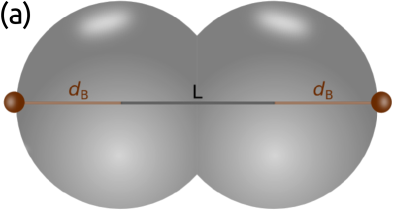
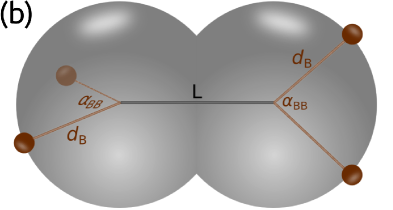
Figure 3: (Color online). Different molecules in $N,P,T$ Monte Carlo simulations: fixed binding sites on the opposite poles, $K_{\textrm{B}}=1$ (a), and more complex geometry with two binding sites on each sphere, $K_{\textrm{B}}=2$ (b). In the last example we set $\alpha_{\textrm{BB}}=\pi/2$ with perpendicular orientation of lines, connecting sites B on each sphere. Center-to-center separation $L$ ($l^{*}=L/\sigma$) and displacement distance $d_{\textrm{B}}=\sigma/2$ were fixed.

3 Results and discussion

3.1 Thermodynamic properties: Theory against Monte Carlo simulations

To test the accuracy of TPT1 we performed $N,P,T$ Monte Carlo simulations for values of $K_{\textrm{B}}$ equal to 1 and 2 (three $l^{*}$ values for each $K_{\textrm{B}}$). We chose to compare the pressure $P$ and the internal energy due to B–B binding, $E^{\textrm{B--B}}$. Since we used the complete A–A association limit within TPT1, the latter quantity, $E^{\textrm{B--B}}$, was the one that could be directly compared to computer simulations. We fixed the temperature $T^{*}=k_{\text{B}}T/\varepsilon=1$, while the pair potential characteristics are given in table 2.

Table 2: Pair potential parameters used for testing TPT1 againt simulations.

$a_{\textrm{BB}}$:	0.1$\sigma$
$\varepsilon_{\textrm{BB}}$:	5.0$\varepsilon$
$d_{\textrm{B}}$:	0.5$\sigma$

The comparison between the theory and simulations is presented in figure 4. We found very good agreement for the pressure, while the theoretical predictions for $E^{\textrm{B--B}}$ were less accurate. In case of $l^{*}=1$ we obtained very good agreement for $K_{\textrm{B}}=1$ and fair agreement for $K_{\textrm{B}}=2$ (black lines and corresponding symbols in $E^{\textrm{B--B}}/N_{\textrm{FS}}k_{\text{B}}T$ sub-figures). If we reduced the $l^{*}$ values (blue and red lines, symbols), the deviations became larger, though the qualitative picture remained correct. Deviations at low $l^{*}$ could be caused by the facts that: (i) fusing of two spheres at small $l^{*}$ is not a small perturbation regarding the reference system of hard spheres, and (ii) the arrangement of binding sites B is fixed during the simulation, which is not the case in TPT1, where the orientation average over all geometries was assumed.

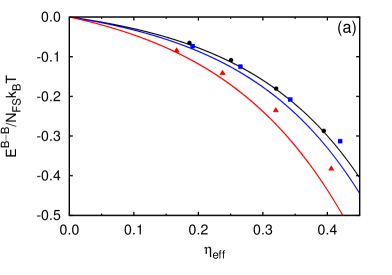
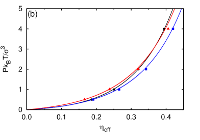
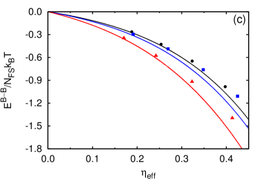
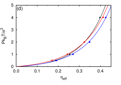
Figure 4: (Color online). Pressure $P$ and association energy $E^{\textrm{B--B}}$ per pair of fused spheres, thus $N_{\textrm{FS}}=N/2$. The calculations are presented by lines and the corresponding simulation results by symbols. We studied three different $l^{*}$ values: 0.2 (red, $\blacktriangle$), 0.6 (blue, $\blacksquare$) and 1.0 (black, $\bullet$). Panels, (a) and (b), belong to $K_{\textrm{B}}=1$ and the panels, (c) and (d), to the case with $K_{\textrm{B}}=2$. Calculation apply to $T^{*}=k_{\text{B}}T/\varepsilon=1$; pair potential parameters are listed in table 2, note that $L=2d_{\textrm{A}}$. Uncertainties of simulation are within the size of symbols.

3.2 Effect of protein’s shape on the liquid-liquid phase diagram

To illustrate the influence of protein shape on the liquid-liquid phase behavior, we compared the phase diagrams for two versions of the model: model (I) of two fused hard spheres and the model (II) of equivalent hard sphere, which was defined as a limiting case of (I), when $L\rightarrow 0$ and $\sigma\rightarrow d_{\textrm{eqv}}$. The latter was chosen in such a way, that the volume of two fused spheres in case (I) was equal to that of the equivalent sphere (II): $d_{\textrm{eqv}}=\sigma\sqrt[3]{1+3l^{*}/2-l{{}^{*}}^{3}/2}$. Example (II) might be interpreted as the usual hard sphere model of diameter $d_{\textrm{eqv}}$, with $2K_{\textrm{B}}$ of sites B, i.e., the same number as on the two fused spheres. In such an interpretation, the A–A contributions to the physical properties can be neglected. Describing the aggregation of fused spheres of diameter $d_{\textrm{eqv}}$ within the limiting conditions $l^{*}\rightarrow 0$ and $D(l^{*})\rightarrow\frac{1}{2}$, where $\eta_{\textrm{eff}}=\eta/2=\pi\rho d_{\textrm{eqv}}^{3}/12=\pi\rho_{\textrm{d}}d_{\textrm{eqv}}^{3}/6$, led us to the model examined in reference [8]. Other parameters and relations between examples (I) and (II) are listed in table 3.

Table 3: Pair potential parameters and relations used in investigation of effects of protein’s shape.

	two fused spheres at $L$ (I)	equivalent sphere (II)
diameter:	$\sigma$	$d_{\textrm{eqv}}=\sigma\sqrt[3]{1+1.5l^{*}-0.5l{{}^{*}}^{3}}$
$\eta_{\textrm{eff}}:$	$D(l^{*})\eta$	$\pi\rho_{\textrm{d}}d_{\textrm{eqv}}^{3}/6$
$\varepsilon_{\textrm{BB}}$:	$\varepsilon$	$\varepsilon$
$d_{\textrm{B}}$:	$\sigma/2$	$d_{\textrm{eqv}}/2$
$a_{\textrm{BB}}$:	0.1$\sigma$	0.1$\sigma$
number of sites B:	$K_{\textrm{B}}$ (per building block)	$2K_{\textrm{B}}$

Figure 5: (Color online). Phase diagrams for different $l^{*}$ values: 0.2 (a), 0.6 (b), and 1.0 (c), color notation is the same as in figure 4. Model of two fused spheres (I) is denoted by dashed lines and the limiting model of equivalent sphere (II) by solid lines. The results apply to three different $K_{\textrm{B}}$ values, written without (I) and within brackets (II), respectively.

In figure 5, we show phase diagrams for the variants (I) and (II) described above, at three $l^{*}$ values and for different numbers of sites B. As observed before [41], an increase of the number of sites B shifts the critical density toward higher values. What is more interesting here is the effect of the separation distance parameter $l^{*}$ on the phase behavior. For a sufficiently small $l^{*}$, i.e., $l^{*}=0.2$ — see figure 5 (a), the difference between the phase diagrams for two versions of the model becomes negligible, regardless of the $K_{\textrm{B}}$ value. If centers of fused spheres are located at larger distance, $l^{*}=0.6$ — see figure 5 (b), the difference becomes more pronounced: both critical temperature and density are lowered. Deviations become the strongest for the limiting example of two spheres fused in contact, that is for $l^{*}=1.0$, cf. figure 5 (c). In this case, the larger number of sites (larger area available for interaction) additionally affects the liquid-liquid phase diagram. The shift toward lower critical densities (or packing fractions) is consistent with experimental studies of the Y-shaped antibodies [12, 13].

4 Conclusions

Proteins come in many shapes, from ellipsoidal to Y-like and are never perfectly spherical as treated by most theoretical models. Further, even in dilute solutions they have a tendency to form dimers and can be represented by two fused spheres. For dense systems close to precipitation, the actual geometry of the protein molecules is important; the inter-particle interactions are directional and of short-range. In the present study, we modify the first-order thermodynamic perturbation theory for associating fluids to be applicable to the models allowing hard-sphere particles to inter-penetrate. These particles can further aggregate. We confront theoretical predictions for thermodynamic properties of the proposed model with predictions of the corresponding Monte Carlo simulations. We obtain an excellent agreement for the pressure and fair agreement for the excess internal energy. Next, we use this model to predict the liquid-liquid phase diagram for protein solutions. We are interested in the effects of protein shape on the phase coexistence curve. We show that the fused hard-sphere model reduces the critical density of the system in comparison with the same quantity calculated for the hard-sphere model. This finding is consistent with experimental observations for Y-shaped antibodies. Using the cloud-point temperature measurements, we currently investigate the influence of various salts on the stability of lactoferrin solutions in water. The latter protein has a shape of two fused spheres, and the hard-sphere model is not a good representation of it. Theoretical approach developed in this paper will be used to analyze experimental data for lactoferrin and some other proteins of non-spherical geometry.

Плин зi спаяних сфер як модель розчину протеїнiв М. Кастелiч${}^{\textsf{\footnotesize{\mbox{?}}}}$, Ю.В. Калюжний${}^{\textsf{\footnotesize{\mbox{?}}}}$, В. Влахi${}^{\textsf{\footnotesize{\mbox{?}}}}$

             
${}^{\textsf{\footnotesize 1}}$ Факультет хiмiї i хiмiчної технологiї, Унiверситет Любляни, вул. Вечна, 113, 1000 Любляна, Словенiя ${}^{\textsf{\footnotesize 2}}$ Iнститут фiзики конденсованих систем НАН України, вул. I. Свєнцiцького, 1, 79011 Львiв, Україна

References

- [1] Gunton J.D., Shiryayev A., Pagan D.L., Protein Condensation: Kinetic Pathways to Crystallization and Disease, Cambridge University Press, Cambridge, 2007.
- [2] Abramo M.C., Caccamo C., Costa D., Pellicane G., Ruberto R., Wanderlingh U., J. Chem. Phys., 2012, 136, No. 3, 035103; doi:10.1063/1.3677186.
-
[3]
Lomakin A., Asherie N., Benedek G.B., Proc. Natl. Acad. Sci. U.S.A.,
1999, 96, No. 17, 9465;
doi:10.1073/pnas.96.17.9465. - [4] Ruppert S., Sandler S.I., Lenhoff A.M., Biotechnol. Progr., 2001, 17, No. 1, 182; doi:10.1021/bp0001314.
- [5] Rosch T.W., Errington J.R., J. Phys. Chem. B, 2007, 111, No. 43, 12591; doi:10.1021/jp075455q.
- [6] Gogelein C., Nagele G., Tuinier R., Gibaud T., Stradner A., Schurtenberger P., J. Chem. Phys., 2008, 129, No. 8, 085102; doi:10.1063/1.2951987.
- [7] Carlsson F., Malmsten M., Linse P., J. Phys. Chem. B, 2001, 105, No. 48, 12189; doi:10.1021/jp012235i.
- [8] Kastelic M., Kalyuzhnyi Yu.V., Hribar-Lee B., Dill K.A., Vlachy V., Proc. Natl. Acad. Sci. U.S.A., 2015, 112, No. 21, 6766; doi:10.1073/pnas.1507303112.
- [9] Lekkerkerker H.N.W., Tuiner R., Colloids and the Depletion Interaction, Lecture Notes in Physics Vol. 833, Springer, Dordrecht, 2011; doi:10.1007/978-94-007-1223-2.
- [10] Taratuta V.G., Holschbach A., Thurston G.M., Blankschtein D., Benedek G.B., J. Phys. Chem., 1990, 94, No. 5, 2140; doi:10.1021/j100368a074.
- [11] Broide M.L., Berland C.R., Pande J., Ogun O.O., Benedek G.B., Proc. Natl. Acad. Sci. U.S.A., 1991, 88, No. 13, 5660; doi:10.1073/pnas.88.13.5660.
-
[12]
Mason B.D., Enk J.Z., Zhang L., Remmele R.L.J., Zhang J., Biophys. J.,
2010, 99, No. 11, 3792;
doi:10.1016/j.bpj.2010.10.040. - [13] Wang Y., Lomakin A., Latypov R.F., Laubach J.P., Hideshima T., Richardson P.G., Munshi N.C., Anderson K.C., Benedek G.B., J. Chem. Phys., 2013, 139, No. 12, 121904; doi:10.1063/1.4811345.
- [14] Yatsenko G., Schweitzer K.S., J. Chem. Phys., 2007, 126, No. 1, 014505; doi:10.1063/1.2405354.
- [15] Liu B.T., Hsu J.P., J. Chem. Phys., 1995, 103, No. 24, 10632; doi:10.1063/1.469849.
- [16] Wheeler M.J., Bertram A.K., Atmos. Chem. Phys., 2012, 12, No. 2, 1189; doi:10.5194/acp-12-1189-2012.
- [17] Wertheim M.S., J. Stat. Phys., 1986, 42, No. 3–4, 459; doi:10.1007/BF01127721.
- [18] Wertheim M.S., J. Stat. Phys., 1986, 42, No. 3–4, 477; doi:10.1007/BF01127722.
- [19] Chapman W.G., Jackson G., Gubbins K.E., Mol. Phys., 1988, 65, No. 5, 1057; doi:10.1080/00268978800101601.
- [20] Li W., Persson B.A., Morin M., Behrens M.A., Lund M., Oskolkova M.Z., J. Phys. Chem. B, 2014, 119, No. 2, 503; doi:10.1021/jp512027j.
- [21] Cummings P.T., Stell G., Mol. Phys., 1984, 51, No. 2, 253; doi:10.1080/00268978700100861.
- [22] Stell G., Zhou Y., J. Chem. Phys., 1989, 91, No. 6, 3618; doi:10.1063/1.456894.
- [23] Kalyuzhnyi Yu.V., Stell G., Llano-Restrepo M.L., Chapman W.G., Holovko M.F., J. Chem. Phys., 1994, 101, No. 9, 7939; doi:10.1063/1.468221.
- [24] Pizio O.A., J. Chem. Phys., 1994, 100, No. 1, 548; doi:10.1063/1.466971.
-
[25]
Kalyuzhnyi Yu.V., Stell G., Holovko M.F., Chem. Phys. Lett., 1995,
235, No. 3–4, 355;
doi:10.1016/0009-2614(95)00106-E. - [26] Duda Yu.J., Kalyuzhnyi Yu.V., Holovko M.F., J. Chem. Phys., 1996, 104, No. 3, 1081; doi:10.1063/1.470763.
- [27] Wertheim M.S., J. Stat. Phys., 1984, 35, No. 1–2, 19; doi:10.1007/BF01017362.
- [28] Wertheim M.S., J. Stat. Phys., 1984, 35, No. 1–2, 35; doi:10.1007/BF01017363.
- [29] Kalyuzhnyi Yu.V., Stell G., Mol. Phys., 1993, 78, No. 5, 1247; doi:10.1080/00268979300100821.
- [30] Ghonazgi D., Chapman W.G., Mol. Phys., 1993, 80, No. 1, 161; doi:10.1080/00268979400101881.
- [31] Ghonazgi D., Chapman W.G., Mol. Phys., 1994, 83, No. 1, 145; doi:10.1080/00268979400101141.
- [32] Duda Yu., Lee L.L., Kalyuzhnyi Yu.V., Chapman W.G., Ting P.D., Chem. Phys. Lett., 2001, 339, No. 1–2, 89; doi:10.1016/S0009-2614(01)00304-9.
-
[33]
Duda Yu., Lee L.L., Kalyuzhnyi Yu.V., Chapman W.G., Ting P.D., J. Chem.
Phys., 2001, 114, No. 19, 8484;
doi:10.1063/1.1363667. - [34] Urbic T., Vlachy V., Kalyuzhnyi Yu.V., Dill K.A., J. Chem. Phys., 2007, 127, No. 17, 174511; doi:10.1063/1.2784124.
- [35] Kalyuzhnyi Yu.V., Hlushak S.P., Cummings P.T., J. Chem. Phys., 2012, 137, No. 24, 244910; doi:10.1063/1.4773012.
- [36] Hansen J.P., McDonald I.R., Theory of Simple Liquids, 3rd Edn., Elsevier, Boston, 2006.
- [37] Wertheim M.S., J. Chem. Phys., 1986, 85, No. 5, 2929; doi:10.1063/1.451002.
- [38] Tildesley D.J., Streett W.B., Mol. Phys., 1980, 41, No. 1, 85; doi:10.1080/00268978000102591.
- [39] Frenkel D., Smit B., Understanding Molecular Simulations: From Algorithms to Applications, Academic Press, London, 1996.
- [40] Streett W.B., Tildesley D.J., Proc. R. Soc. London, Ser. A, 1976, 348, No. 1655, 485; doi:10.1098/rspa.1976.0051.
-
[41]
Bianchi E., Largo J., Tartaglia P., Zaccarelli E., Sciortino F.,
Phys. Rev. Lett., 2006, 97, No. 16, 168301;
doi:10.1103/PhysRevLett.97.168301.