Beyond the Melnikov method: a computer assisted approach

Abstract

We present a Melnikov type approach for establishing transversal intersections of stable/unstable manifolds of perturbed normally hyperbolic invariant manifolds (NHIMs). The method is based on a new geometric proof of the normally hyperbolic invariant manifold theorem, which establishes the existence of a NHIM, together with its associated invariant manifolds and bounds on their first and second derivatives. We do not need to know the explicit formulas for the homoclinic orbits prior to the perturbation. We also do not need to compute any integrals along such homoclinics. All needed bounds are established using rigorous computer assisted numerics. Lastly, and most importantly, the method establishes intersections for an explicit range of parameters, and not only for perturbations that are ‘small enough’, as is the case in the classical Melnikov approach.

Keywords and phrases: Melnikov method, normally hyperbolic invariant manifolds, whiskered tori, transversal homoclinic intersection, computer assisted proof

AMS classification numbers: 37D10, 58F15 ,65G20

1 Introduction

The presence of the transversal intersection between stable and unstable manifolds for fixed point or periodic orbit is one of the main technical tools used to prove the chaotic behavior of the deterministic dynamical system (see for example [15] and the literature given there). In the context of the small perturbations of an integrable system the basic analytical technique used to establish the transversality is the Melnikov method [21] introduced in 1963. V.I. Arnold generalized these ideas to produce the first example of what is now called Arnold Diffusion [1]. In fact the (now widely-used) Melnikov function (see for example [25, 17]) is, up to a constant, exactly the integral that Poincaré derived from Hamilton-Jacobi theory to obtain his obstruction to integrability in the restricted three body problem in [24].

Melnikov type methods are based on investigating integrals along homoclinic orbits to normally hyperbolic invariant manifolds (NHIMs) [8, 10, 11, 17, 21, 25]. There are natural problems with such approach: It is very rarely the case that one can establish analytic formulae for such homoclinics. In most cases they are not known, and then computing integrals along them is impossible. The second problem is that even if one has an analytic formula for the homoclinic, the integral in question can be very hard to compute. In most real life systems such integrals would not be expressed through simple formulas.

We resolve these two problems the following way. Firstly, we investigate the dependence of the manifolds on the parameter using geometric and computer assisted tools. The slopes of the manifolds depending on the parameter follow from cone condition type bounds in the state space extended by the parameters. Second order derivatives also follow from geometric structures. This way we obtain bounds on the stable and unstable manifolds of NHIMs, together with their dependence up to second order on the perturbation parameter. We then propagate these bounds using rigorous (interval based) integration up to a section where they meet. Based on the bounds, and in particular using the dependence on the manifolds on the perturbation parameter, we establish transversal intersections for a given, explicit, range of perturbations. The range is large enough so that for the larger parameters from the range we can detect the transversal intersections directly, and continue to higher perturbations using standard techniques.

Our contribution to the existing theory is twofold:

Firstly, in this paper we develop a method for establishing centre unstable manifolds of NHIMs, in the context of ordinary differential equations. The main benefit from our approach is that we do not need to assume that the NHIM exists in order to apply our method. (Our method is constructive, not perturbative.) We formulate assumptions, which guarantee the existence of a center-unstable manifold within an investigated neighborhood. The assumptions of our theorem depend only on the bounds on the first derivative of the vector field. These guarantee that the center-unstable manifold exists, and is a graph of a function within the investigated region. The method gives explicit bounds on the slope of the manifold. Moreover, by considering bounds on the second derivative of the vector field, we obtain explicit estimates on the second order derivatives of the center-unstable manifold. By changing the sign of the vector field, the method establishes existence of center-stable manifolds. By intersecting the center-stable manifold with the centre-unstable manifold we establish the existence of a NHIM within the investigated region. Our method also establishes bounds on the first and second order dependence of the manifolds on the parameters for families of ODEs. Summing up: the method is explicit, establishes existence of the manifolds over a specified, macroscopic domain, all assumptions can be verified from simple estimates on the first and second derivative of the vector field, and gives explicit estimates on the dependence of the manifolds on parameters.

Our second contribution is developing a Melnikov-type theory for establishing transversal intersections of stable/unstable manifolds of NHIMs. The method is based on interval arithmetic integration of ODEs and propagation of local bounds on the manifolds up to the point of their intersection. The benefit from our approach is the following. We do not have to know any analytic formulae for the homoclinics. They are established using rigorous computer assisted numerics. Secondly, we do not need to compute any integrals. All bounds on the manifolds are propagated by our integrator in form of rigorous, interval arithmetic bounds for the jets. This method allows us to establish intersections of the manifolds for specific ranges of parameters. These ranges are large enough to later continue the proof of the intersections of the manifolds using standard continuation arguments.

We emphasize that, to the best of our knowledge, this is the first computer assisted Melnikov type method, which works over an explicit parameter range. Since our method does not rely on analytic computations along homoclinics, we believe that our approach is very versatile and can be applied to numerous problems that are not accessible to the standard methods.

The paper is organized as follows. We first address the problem how to establish transversal intersections of manifolds for given ranges of perturbation parameters, under the assumption that we have bounds on the first and second derivatives of the stable/unstable manifolds of NHIMs. This problem is introduced below in subsection 1.1, and the main idea behind our approach is explained in subsection 1.2. We then follow up with full details in section 3, where the formulation is made precise and the main results are proven. Secondly, we address how to establish the needed bounds for the derivatives of stable/unstable manifolds. In section 4 we recall the results from [6], where such bounds are established in the setting of discrete dynamical systems. In section 4 we also extend the method to obtain explicit bounds on second derivatives of the manifolds. In section 5 we further extend the results from section 4 to the setting of ODEs. We make sure that the needed assumptions follow from the bounds on the vector field, so that we do not have to integrate the ODEs. As the by-product we obtain also a generalization of results from [6] about establishing of NHIM for ODEs. In section 6 we give an example of application of our method.

An alternative to [6] and its extension presented in this paper for obtaining bounds on derivatives of stable/unstable manifolds of NHIMs, is the parameterization method [2]. This method is suitable for application to computer assisted proofs. (For examples of such applications see [3, 7, 14, 19, 22], amongst others.) We believe that our approach to Melnikov method (from sections 1.1, 1.2, and 3) could also be successfully combined with [2]. We decide to use the geometric method [6] and its generalization to ODEs, since it does not require high order expansions in order to establish existence of the manifolds, but follows from direct estimates on first and second derivatives of the vector field.

In the two subsections that follow we specify the setup under which our paper is written and outline the main idea.

1.1 The setup

In this section we formulate our main goals and set up the notation. The problem is formulated in the simplest possible setting. We consider a non-autonomous perturbation of an autonomous ODE on the plane. This enables us to present the main features. Our method though can be applied in a much more general setting.

We consider a vector field

$$f_{0}:\mathbb{R}^{2}\rightarrow\mathbb{R}^{2},$$

and a function

$$g:\mathbb{R}^{2}\times\mathbb{R}\times\mathbb{R}\rightarrow\mathbb{R}^{2}.$$

We assume that $g$ is $2\pi$ periodic in the last coordinate. We shall consider the following family of time periodic ODEs

$$\left(x,y\right)^{\prime}=f_{\varepsilon}\left(x,y,t\right)=f_{0}\left(x,y\right)+g\left(x,y,\varepsilon,t\right).$$ (1)

We assume that for $\varepsilon=0$ holds $g\left(x,y,0,t\right)=0$. This means that we treat $g$ as a perturbation, with $\varepsilon$ being the perturbation parameter.

We shall assume that for $\varepsilon=0,$ (1) has a hyperbolic fixed point $\left(x_{0},y_{0}\right)$ and that we have a homoclinic orbit along the stable/unstable manifold of $\left(x_{0},y_{0}\right)$.

Since the fixed point is hyperbolic, for $\varepsilon\neq 0$ it will be perturbed to a $2\pi$ periodic hyperbolic orbit. We shall use a notation $\gamma_{\varepsilon}\left(t\right)$ for this orbit and assume that such orbits exist for $\varepsilon\in E$, where $E\subset\mathbb{R}$ is a closed interval around zero.

In order to investigate the intersections of the stable/unstable manifolds of $\gamma_{\varepsilon}$ we consider a section $\Sigma$, which is transversal to the homoclinic orbit (which exists for $\varepsilon=0$). For $\varepsilon\geq 0$, the stable manifold of $\gamma_{\varepsilon}$ for the problem (1), with initial condition starting at time $\tau$ will hit $\Sigma$ at a point, which we denote as $p^{s}\left(\varepsilon,\tau\right)$. Similarly, by $p^{u}\left(\varepsilon,\tau\right)$ we denote the point of intersection of the unstable manifold with $\Sigma$.

Remark 1

The construction of the points $p^{s}\left(\varepsilon,\tau\right)$, $p^{u}\left(\varepsilon,\tau\right)$ is made precise and carried out in full detail in section 3.1. Figure 1 gives a graphical illustration of the setup.

We then define the (signed) distance $\delta$ between the two manifolds on $\Sigma$ as

$$\delta\left(\varepsilon,\tau\right):=p^{u}\left(\varepsilon,\tau\right)-p^{s}\left(\varepsilon,\tau\right).$$ (2)

The main question is to establish conditions on $\delta\left(\varepsilon,\tau\right)$ that ensure that the stable/unstable manifolds of such orbits intersect transversally, for all $\varepsilon\in E\setminus\{0\}$.

The above setting, in which we are perturbing a fixed point, is the simplest one. In general we could be interested in intersections of stable/unstable manifolds of perturbed NHIMs. The tools for establishing such manifolds and their perturbations, together with all the ingredients needed to apply our method are developed in [6] and its generalization to ODEs form section 5. There are no obstacles to generalizing to such setting. We restrict ourselves though to the simplest case for the sake of clarity of exposition and postpone detailed treatment of the general case for NHIMs for later publication.

1.2 The main idea in simplest terms

We consider a $C^{2}$ function $\delta:\mathbb{R\times S}^{1}\rightarrow\mathbb{R}$, which is defined in (2). Since for $\varepsilon=0$ the stable and unstable manifolds coincide forming a homoclinic orbit, we know that

$$\delta\left(0,\tau\right)=0\qquad\text{for all }\tau\in\mathbb{S}.$$

For fixed $\varepsilon\in\mathbb{R}$ we will use the notation

$$\delta_{\varepsilon}\left(\tau\right):=\delta\left(\varepsilon,\tau\right).$$

Let $E$ be a closed interval in $\mathbb{R}$, which contains zero. Our aim is to give a simple set of assumptions that will lead to a conclusion that for any $\varepsilon\in E\setminus\{0\}$ the function $\delta_{\varepsilon}$ will have nontrivial zeroes. In other words, that there exists a $\xi\left(\varepsilon\right)\in\mathbb{S}^{1}$ such that

$$\delta_{\varepsilon}\left(\xi\left(\varepsilon\right)\right)=0,\qquad\frac{d\delta_{\varepsilon}}{d\tau}\left(\xi\left(\varepsilon\right)\right)\neq 0.$$

For $A\subset\mathbb{R\times S}^{1}$ we shall write

$$\left[\frac{\partial\delta}{\partial\varepsilon}\left(A\right)\right]:=\left[\inf_{\left(\varepsilon,\tau\right)\in A}\frac{\partial\delta}{\partial\varepsilon}\left(\varepsilon,\tau\right),\sup_{\left(\varepsilon,\tau\right)\in A}\frac{\partial\delta}{\partial\varepsilon}\left(\varepsilon,\tau\right)\right].$$

Our idea is based on the fact that for any $\varepsilon\in E\setminus\{0\}$

$$\frac{\delta_{\varepsilon}\left(\tau\right)}{\varepsilon}\in\left[\frac{\partial\delta}{\partial\varepsilon}\left(E\times\left\{\tau\right\}\right)\right].$$ (3)

This means that if we can establish that for some $\tau_{1},\tau_{2}\in\mathbb{S}^{1}$

$$\left[\frac{\partial\delta}{\partial\varepsilon}\left(E\times\left\{\tau_{1}\right\}\right)\right]<0<\left[\frac{\partial\delta}{\partial\varepsilon}\left(E\times\left\{\tau_{2}\right\}\right)\right],$$ (4)

then for any $\varepsilon\in E\setminus\{0\}$, by (3) and (4),

$$\frac{\delta_{\varepsilon}\left(\tau_{1}\right)}{\varepsilon}<0<\frac{\delta_{\varepsilon}\left(\tau_{2}\right)}{\varepsilon}.$$

Hence, by the Bolzano theorem, there exists a $\xi\left(\varepsilon\right)\in\left[\tau_{1},\tau_{2}\right]$, such that

$$\delta_{\varepsilon}\left(\xi\left(\varepsilon\right)\right)=0.$$

If in addition to (4) we have that

$$\left[\frac{\partial^{2}\delta}{\partial\tau\partial\varepsilon}\left(E\times\left[\tau_{1},\tau_{2}\right]\right)\right]>0,$$ (5)

then for any $\tau\in\left[\tau_{1},\tau_{2}\right]$

$$\frac{d}{d\tau}\left(\frac{\delta_{\varepsilon}\left(\tau\right)}{\varepsilon}\right)\in\left[\frac{\partial^{2}\delta}{\partial\tau\partial\varepsilon}\left(E\times\left[\tau_{1},\tau_{2}\right]\right)\right]>0.$$

Thus, for each $\varepsilon\in E\setminus\{0\},$ the point $\xi\left(\varepsilon\right)$ is unique and

$$\frac{d\delta_{\varepsilon}}{d\tau}\left(\xi\left(\varepsilon\right)\right)\neq 0.$$

To sum up the above discussion, in order to show that for any $\varepsilon\in E\setminus\{0\}$ we have nontrivial zeros of the function $\delta_{\varepsilon}$, it is sufficient to verify (4) and (5). We emphasize that in this approach we have an explicit range $E$ of $\varepsilon$ for which the nontrivial zeros exist.

Summing up, to compute the Melnikov distance $\delta$, our method combines two ingredients, both computer assisted:

• the geometric method to establish explicit bounds for normally hyperbolic invariant manifolds and their stable and unstable fibers, together with their dependence on parameter.

• the rigorous $C^{2}$-integration of our system away from the NHIM.

This method can be generalized to many dimensions.

2 Preliminaries

2.1 Notations and conventions

We will use the Euclidian norm unless stated otherwise. For two vectors $z_{1},z_{2}$ we denote their scalar product by $(z_{1}|z_{2})$. For a matrix $A$, by $A^{\top}$ we denote the transpose of $A$. By $I$ we will denote the identity matrix, the dimension will be known from the context.

For a set $A$, we shall use $A^{c}$ to denote its complement.

For a function $f:\mathbb{R}^{n}\rightarrow\mathbb{R}^{m}$ for $z_{1},z_{2}\in\mathbb{R}^{n}$ we define an average of $f$ on the segment $[z_{1},z_{2}]$ by

$$\overline{f}(z_{1},z_{2})=\int_{0}^{1}f(z_{1}+s(z_{2}-z_{1}))ds.$$

Observe that we have the following equality for $f\in C^{1}$:

$$f(z_{2})-f(z_{1})=\overline{Df}(z_{1},z_{2})(z_{2}-z_{1}).$$

2.2 Logarithmic norms and related topics

In this section we state some facts about logarithmic norms [9, 20, 16, 18] and some analogous notions. These are later used in section 5. Since the results are of technical nature, we give their proofs in the appendix.

Definition 2

For a square matrix $A\in\mathbb{R}^{n\times n}$ we define $m(A)$ by

$$m(A)=\min_{z\in\mathbb{R}^{n},\|z\|=1}\|Az\|,$$

the logarithmic norm of $A$ denoted by $l(A)$ by [20, 9, 16, 18]

$$l(A)=\lim_{h\rightarrow 0^{+}}\frac{\|I+hA\|-\|I\|}{h}$$ (6)

and the logarithmic minimum of $A$

$$m_{l}(A)=\lim_{h\rightarrow 0^{+}}\frac{m(I+hA)-\|I\|}{h}.$$ (7)

It is easy to see that if $A$ is invertible, then

$$m(A)=\frac{1}{\|A^{-1}\|},$$

otherwise $m(A)=0$.

It is known that $l(A)$ is a convex function.

Lemma 3

The limit in the definition of $m_{l}(A)$ exists and

$$m_{l}(A)=-l(-A).$$ (8)

Moreover, the convergence to this limit is locally uniform with respect to $A$ and $m_{l}(A)$ is a concave function.

Proof. See Appendix 8.1.   

Below theorem establishes a bound on distances of solutions of an ODE in terms of the logarithmic norm. The proof of this result can be found in [16].

Theorem 4

Consider an ODE

$$x^{\prime}=f(t,x),$$ (9)

where $x\in\mathbb{R}^{n}$ and $f:\mathbb{R}\times\mathbb{R}^{n}\rightarrow\mathbb{R}^{n}$ is $C^{1}$.

Let $x(t)$ and $y(t)$ for $t\in[t_{0},t_{0}+T]$ be two solutions of (9). Let $W\subset\mathbb{R}^{n}$ such that for each $t\in[t_{0},t_{0}+T]$ the segment connecting $x(t)$ and $y(t)$ is contained in $W$. Let

$$L=\sup_{x\in W,t\in[t_{0},t_{0}+T]}l\left(\frac{\partial f}{\partial x}(t,x)\right).$$

Then for $t\in[0,T]$ holds

$$\left\|x(t_{0}+t)-y(t_{0}+t)\right\|\leq\exp(Lt)\left\|x(t_{0})-y(t_{0})\right\|.$$

Theorem 4 gives an upper bound for the distance between solutions of an ODE. We now show a similar result, which allows us to obtain a lower bound.

Theorem 5

Consider an ODE

$$x^{\prime}=f(x),$$ (10)

where $x\in\mathbb{R}^{n}$ and $f:\mathbb{R}^{n}\rightarrow\mathbb{R}^{n}$ is $C^{1}$.

Let $x(t)$ and $y(t)$ for $t\in[0,T]$ be two solutions of (10). Let $W\subset\mathbb{R}^{n}$ be such that for each $t\in[0,T]$ the segment connecting $x(t)$ and $y(t)$ is contained in $W$. Let

$$m_{l}(Df,W)=\inf_{x\in W}m_{l}(Df(x)).$$

Then for $t>0$ holds

$$\|x(t)-y(t)\|\geq\exp(m_{l}(Df,W)t)\|x(0)-y(0)\|.$$

Proof. See Appendix 8.2.   

In above results the choice of norms was arbitrary. We will apply these results in the case when the norm is Euclidean. In such case we have the following results.

Lemma 6

For the Euclidian norm holds

$$l(A) = \max\{\lambda\in\text{spectrum of }(A+A^{\top})/2\}$$ (11)

$$m_{l}(A) = \min\{\lambda\in\text{spectrum of }(A+A^{\top})/2\}.$$ (12)

Proof. The formula (11) is well known [16]. From Lemma 3, $m_{l}(A)=-l(-A)$, which gives (12).   

Lemma 7

Consider the Euclidean norm $\left\|\cdot\right\|$. Assume that $A\in W$, where $W\subset\mathbb{R}^{n\times n}$ is compact. Assume also that $h\in(0,h_{0}]$. Then

$$\|I+hA\|=1+hl(A)+r(h,A),$$

where

$$\|r(h,A)\|\leq Mh^{2},$$

for some constant $M=M(h_{0},W)$ (the constant $M$ depends on $h_{0}$ and $W$).

Proof. See Appendix 8.3.   

Lemma 8

Assume that $A\in W$, where $W\subset\mathbb{R}^{n\times n}$ compact. Assume $h\in(0,h_{0}]$. Then

$$m(I+hA)=1+hm_{l}(A)+r(h,A)$$

where

$$\|r(h,A)\|\leq Mh^{2}$$

for some constant $M=M(h_{0},W)$ (the constant $M$ depends on $h_{0}$ and $W$).

Proof. See Appendix 8.4.   

3 Melnikov type method

In this section we introduce a Melnikov type method. The difference with the standard approach is that we do not integrate along the homoclinic orbit. Instead, we assume that we have bounds on the local parameterizations of the stable/unstable manifold of the perturbed orbit. These are then propagated to the section where we measure the distance. This formulation allows us to verify our assumptions for a given range of perturbations. We do not need to assume that the perturbation is small enough.

While presenting the method, we make a number of assumptions about the stable and unstable manifolds. Namely that we have their parameterization, and that we have bounds on their derivatives. Based on these assumptions we formulate our results. We emphasize straightaway that we know how to obtain such bounds. This is the subject of subsequent sections.

In section 3.1 we present the method; in particular Theorem 9, which contains the main result. In section 3.2 we discuss how to verify the assumptions, based on the bounds on the derivatives of the parametrizations of the stable and unstable manifolds. How such bounds can be obtained is presented in section 5.

3.1 The method

In our treatment of the problem we shall consider the following formulation of (1), in a state space that is extended to include both the time and the parameter:

$$x^{\prime} =\pi_{x}f_{\varepsilon}\left(x,y,s\right),$$

$$y^{\prime} =\pi_{y}f_{\varepsilon}\left(x,y,s\right),$$ (13)

$$\varepsilon^{\prime} =0,$$

$$s^{\prime} =1.$$

In the extended phase space coordinates $q=(x,y,\varepsilon,s),$ we shall use the notation

$$q^{\prime}=f(q),$$ (14)

for the ODE (13), where

$$f:\mathbb{R}^{3}\times\mathbb{S}^{1}\rightarrow\mathbb{R}^{4}.$$

We shall write $\Phi_{t}(q)$ for the flow of (14).

We will refer to the cyclic variable $s$ as $s$-time or just a time. There will be also other ‘time’ occasionally appearing in our discussion, this will be the time along the solution of the system (14), we will refer this variable as $t$-time. Given two points on the trajectory of (14) the $t$-time between them will be the difference between $s$-times of these two points.

The family of periodic orbits $\gamma_{\varepsilon}(s)$ forms a two dimensional invariant manifold (with a boundary) for (14):

$$\Lambda=\left\{\left(\gamma_{\varepsilon}\left(s\right),\varepsilon,s\right):\varepsilon\in E,s\in\mathbb{S}^{1}\right\}.$$

(The boundary of $\Lambda$ is $\partial\Lambda=\left\{\left(\gamma_{\varepsilon}\left(s\right),\varepsilon,s\right):\varepsilon\in\partial E,s\in\mathbb{S}^{1}\right\}.$)

For any fixed $\varepsilon\in E$, we shall write

$$\Lambda_{\varepsilon}=\left\{\left(\gamma_{\varepsilon}\left(s\right),e,s\right):e=\varepsilon,s\in\mathbb{S}^{1}\right\},$$

to denote the invariant set containing the periodic orbit of (1), in the extended phase space.

Let $N$ be a set in $\mathbb{R}^{3}\times\mathbb{S}^{1}$ containing $\Lambda$. We shall use $W_{\mathrm{loc}}^{s}\left(\Lambda\right)$ and $W_{\mathrm{loc}}^{u}\left(\Lambda\right)$ to denote the local stable and unstable manifolds in $N$, respectively i.e.

$$W_{\mathrm{loc}}^{s}\left(\Lambda\right) = \left\{q:\Phi_{t}(q)\in N\text{ for all }t\geq 0\right\},$$

$$W_{\mathrm{loc}}^{u}\left(\Lambda\right) = \left\{q:\Phi_{t}(q)\in N\text{ for all }t\leq 0\right\}.$$

(Since the set $N$ will be fixed, we do not include it in our notations for the local manifolds.) We assume that in the neighborhood $N$ we can parameterize $W_{\mathrm{loc}}^{u}\left(\Lambda\right)$ by a function

$$w^{u}:\left[-r_{u},r_{u}\right]\times E\times\mathbb{S}^{1}\rightarrow\mathbb{R}^{3}\times\mathbb{S}^{1},$$

where $r_{u}\in\mathbb{R}^{+}$. We also assume that $W_{\mathrm{loc}}^{s}\left(\Lambda\right)$ is parameterized by

$$w^{s}:\left[-r_{s},r_{s}\right]\times E\times\mathbb{S}^{1}\rightarrow\mathbb{R}^{3}\times\mathbb{S}^{1},$$

for $r_{s}\in\mathbb{R}^{+}$. We assume that our parameterizations satisfy

$$\pi_{\varepsilon,s}w^{\iota}\left(r,\varepsilon,s\right)=\left(\varepsilon,s\right),\qquad\text{for }\iota\in\left\{s,u\right\}.$$ (15)

We shall use notations $W^{u}\left(\Lambda\right),$ $W^{s}(\Lambda)$ for the unstable and stable manifolds of $\Lambda$, respectively.

The existence of the manifolds within the set $N$, together with the fact that they are graphs of the functions $w^{u}$ and $w^{s}$, will follow from our construction. Namely, in sections 4 and 5 we present a detailed method which ensures, using constructive arguments, that above assumptions are fulfilled within an explicitly given set $N$.

Let $\Sigma\subset R^{3}\times S^{1}$ be a $3$-dimensional section for (14), such that for any $q\in w^{u}\left((0,r_{u}]\times E\times\mathbb{S}^{1}\right)$ the first intersection for time $t>0$ of the trajectory $\Phi_{t}\left(q\right)$ with $\Sigma$ is transversal. We also assume that for any $q\in w^{s}\left((0,r_{s}]\times E\times\mathbb{S}^{1}\right)$ the first intersection for time $t<0$ of the trajectory $\Phi_{t}\left(q\right)$ with $\Sigma$ is transversal. For simplicity, without loss of generality, we shall assume that $\Sigma=\left\{y=0\right\}$, hence the coordinates on $\Sigma$ are $\left(x,\varepsilon,s\right)$ (see Figure 1).

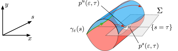
Figure 1: The perturbed orbit $\gamma_{\varepsilon}(s)$ in green (which coincides with $\Lambda_{\varepsilon}$), its unstable manifold in blue and stable manifold in red. The two points on $\Sigma=\{y=0\}$ are $p^{u}\left(\varepsilon,\tau\right):=P^{u}\left(w^{u}\left(r_{u},\varepsilon,\kappa^{u}\left(\varepsilon,\tau\right)\right)\right)$ and $p^{s}\left(\varepsilon,\tau\right):=P^{s}\left(w^{s}\left(r_{s},\varepsilon,\kappa^{s}\left(\varepsilon,\tau\right)\right)\right)$. In red, we have the trajectory along the solution of the ODE, which leads to $p^{u}\left(\varepsilon,\tau\right)$. The (signed) distance between $p^{u}\left(\varepsilon,\tau\right)$ and $p^{s}\left(\varepsilon,\tau\right)$ is the $\delta\left(\varepsilon,\tau\right)$.

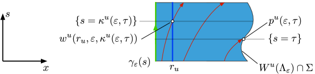
Figure 2:

Figure 3: The perturbed orbit $\gamma_{\varepsilon}(s)$ (which coincides with $\Lambda_{\varepsilon}$) in green and its unstable manifold in blue, projected onto the $x,s$ coordinates. The curled right edge of the blue region is the intersection of the unstable manufold with $\Sigma$. If we start from the point $w^{u}\left(r_{u},\varepsilon,\kappa^{u}\left(\varepsilon,\tau\right)\right)$, which is at an $r_{u}$ distance from $\gamma_{\varepsilon}(s)$, and whose $s$-time is $\kappa^{u}\left(\varepsilon,\tau\right)$, then we will reach $p^{u}\left(\varepsilon,\tau\right):=P^{u}\left(w^{u}\left(r_{u},\varepsilon,\kappa^{u}\left(\varepsilon,\tau\right)\right)\right)$ along a trajectory of the ODE (depicted in red).

Let $\tau^{u}(q)$ and $\tau^{s}\left(q\right)$ stand for

$$\tau^{u}\left(q\right) =\pi_{s}q+\inf\left\{t>0:\Phi_{t}\left(q\right)\in\Sigma\right\},$$ (16)

$$\tau^{s}\left(q\right) =\pi_{s}q+\sup\left\{t<0:\Phi_{t}\left(q\right)\in\Sigma\right\}.$$

Therefore $\tau^{u}(q)$ is the $s$-time coordinate of the point from the first intersection of $\Sigma$ with the forward trajectory of point $q$. Then $\tau^{u}(q)-\pi_{s}q$ is the $t$-time needed for $q$ to reach the section $\Sigma$. For the $\tau^{s}(q)$ we have analogous interpretation.

Let $P^{u}\$and $P^{s}$ be maps defined as

$$P^{u}\left(q\right) =\Phi_{\tau^{u}\left(q\right)-\pi_{s}q}\left(q\right),$$

$$P^{s}\left(q\right) =\Phi_{\tau^{s}\left(q\right)-\pi_{s}q}\left(q\right).$$

The domains of $P^{u}\$and $P^{s}$ are subsets of $\mathbb{R}^{2}\times E\times\mathbb{S}^{1}$, which contain $w^{u}\left(\left(0,r_{u}\right]\times E\times\mathbb{S}^{1}\right)$ and $w^{s}\left(\left(0,r_{s}\right]\times E\times\mathbb{S}^{1}\right)$, respectively. Observe that

$$\pi_{s}P^{u}\left(q\right)=\tau^{u}\left(q\right)\qquad\text{and}\qquad\pi_{s}P^{s}\left(q\right)=\tau^{s}\left(q\right).$$ (17)

We shall assume that for any $\tau$ we can solve the following implicit equations for functions $\kappa^{u},\kappa^{s}:E\times\mathbb{S}^{1}\rightarrow\mathbb{S}^{1}$:

$$\tau^{u}\left(w^{u}\left(r_{u},\varepsilon,\kappa^{u}\left(\varepsilon,\tau\right)\right)\right) =\tau,$$ (18)

$$\tau^{s}\left(w^{s}\left(r_{s},\varepsilon,\kappa^{s}\left(\varepsilon,\tau\right)\right)\right) =\tau.$$ (19)

Function $\kappa^{u}(\varepsilon,\tau)$ gives the $s$-time of the point on the unstable manifold with the unstable parameter $r_{u}$ that reaches the section $\Sigma$ in the $s$-time equal to $\tau$ (see Figure 3).

The questions related to the solvability of (18),(19) are discussed in Remark 11. We define the distance function $\delta:E\times\mathbb{S}^{1}\rightarrow\mathbb{R}$:

$$\delta\left(\varepsilon,\tau\right):=\pi_{x}p^{u}\left(\varepsilon,\tau\right)-\pi_{x}p^{s}\left(\varepsilon,\tau\right),$$ (20)

where

$$p^{\iota}\left(\varepsilon,\tau\right):=P^{\iota}\left(w^{\iota}\left(r_{\iota},\varepsilon,\kappa^{\iota}\left(\varepsilon,\tau\right)\right)\right)\qquad\qquad\text{for }\iota\in\left\{s,u\right\}.$$ (21)

The $\delta$ will play the key role in our derivations. It will turn out that $\delta(\varepsilon,\tau)$ measures the (signed) distance between the intersections of $W^{u}(\Lambda_{\varepsilon})\cap\{s=\tau\}$ and $W^{s}(\Lambda_{\varepsilon})\cap\{s=\tau\}$ on $\Sigma$.

We now formulate our main result.

Theorem 9

Assume that there exists $\tau_{1},\tau_{2}\in\mathbb{S}^{1}$ such that for any $\varepsilon\in E$

$$\frac{\partial}{\partial\varepsilon}\delta\left(\varepsilon,\tau_{1}\right)<0,\qquad\frac{\partial}{\partial\varepsilon}\delta\left(\varepsilon,\tau_{2}\right)>0.$$ (22)

Then for any $\varepsilon\in E\setminus\{0\}$ there exists $\tau^{\ast}\left(\varepsilon\right)\in\left(\tau_{1},\tau_{2}\right)$ such that $W^{u}\left(\Lambda_{\varepsilon}\right)$ and $W^{s}\left(\Lambda_{\varepsilon}\right)$ intersect at a point $q\left(\varepsilon\right)\in\Sigma$, for which $\pi_{\left(\varepsilon,\tau\right)}q\left(\varepsilon\right)=\left(\varepsilon,\tau\right).$

Moreover, if in addition

$$\frac{\partial^{2}}{\partial\tau\partial\varepsilon}\delta\left(\varepsilon,\tau\right)>0,\qquad\text{for any }\varepsilon\in E\text{ and }\tau\in\left(\tau_{1},\tau_{2}\right),$$ (23)

then $q(\varepsilon)$ is uniquely defined and for any fixed $\varepsilon\in E\setminus\{0\}$, the manifolds $W^{u}\left(\Lambda_{\varepsilon}\right)$ and $W^{s}\left(\Lambda_{\varepsilon}\right)$ intersect transversally at $q\left(\varepsilon\right)$; the transversality is considered in the $x,y,s$ coordinates.

Proof. Let us fix $\varepsilon$ and $\tau,$ and define two points

$$q^{\iota}=q^{\iota}\left(\varepsilon,\tau\right)=P^{\iota}\left(w^{\iota}\left(r_{\iota},\varepsilon,\kappa^{\iota}\left(\varepsilon,\tau\right)\right)\right)\qquad\text{for }\iota\in\left\{u,s\right\}.$$ (24)

By definition $q^{u},q^{s}\in\Sigma$. Moreover, by definition of $\kappa^{\iota}\left(\varepsilon,\tau\right)$ (see (18– 19))

$$\pi_{\left(\varepsilon,s\right)}q^{u}=\left(\varepsilon,\tau\right)=\pi_{\left(\varepsilon,s\right)}q^{s}.$$

Moreover, by the definition of $\delta$, we also have

$$\pi_{x}\left(q^{u}-q^{s}\right)=\delta\left(\varepsilon,\tau\right).$$

We therefore see that to establish that $q^{u}=q^{s}$ it is sufficient to check that $\delta\left(\varepsilon,\tau\right)=0$.

If $\varepsilon=0$, then, since for the unperturbed problem we have a homoclinic orbit, for any $\tau\in\mathbb{S}^{1}$

$$\delta(\varepsilon=0,\tau)=0.$$

We have

$$\delta(\varepsilon,\tau) =\delta\left(0,\tau\right)+\int_{0}^{1}\frac{d}{dx}\delta\left(x\varepsilon,\tau\right)dx$$

$$=\varepsilon\int_{0}^{1}\frac{\partial}{\partial\varepsilon}\delta\left(x\varepsilon,\tau\right)dx.$$ (25)

From our assumptions it therefore follows that for any $\varepsilon\in E\setminus\{0\}$

$$\delta\left(\varepsilon,\tau_{1}\right)<0,\qquad\qquad\delta\left(\varepsilon,\tau_{2}\right)>0.$$

By the Bolzano intermediate value theorem (applied to $\tau\rightarrow\delta\left(\varepsilon,\tau\right)$), for any $\varepsilon\in E$ there needs to be a $\tau^{\ast}\left(\varepsilon\right)$ in $\left(\tau_{1},\tau_{2}\right)$, such that

$$\delta\left(\varepsilon,\tau^{\ast}\left(\varepsilon\right)\right)=\pi_{x}\left(q^{u}\left(\varepsilon,\tau^{\ast}\left(\varepsilon\right)\right)-q^{s}\left(\varepsilon,\tau^{\ast}\left(\varepsilon\right)\right)\right)=0,$$

hence the manifolds intersect at $q^{u}\left(\varepsilon,\tau^{\ast}\left(\varepsilon\right)\right)=q^{s}\left(\varepsilon,\tau^{\ast}\left(\varepsilon\right)\right).$

We now prove the transversality. As a consequence of the transversality we obtain the uniqueness of $q(e)$. Let us fix $e\in E\setminus\{0\}$. Observe that since

$$\frac{\partial}{\partial\tau}\delta\left(e,\tau\right)=e\int_{0}^{1}\frac{\partial^{2}}{\partial\tau\partial\varepsilon}\delta\left(xe,\tau\right)dx\neq 0,\quad\tau\in(\tau_{1},\tau_{2})$$

the intersection parameter $\tau^{\ast}(\varepsilon)$ is uniquely defined. Let $q(e)$ denotes the intersection point

$$q(e)=q^{u}(e,\tau^{\ast}(e))=q^{s}(e,\tau^{\ast}(e)).$$

We consider the transversality in the coordinates $y,x,s$.

Let $w=f\left(q\left(e\right)\right)$. Since $q\left(e\right)\in W^{s}\left(\Lambda\right)\cap W^{u}\left(\Lambda\right)$, we have

$$w\in T_{q\left(e\right)}W^{s}\left(\Lambda\right)\qquad\text{and\qquad}w\in T_{q\left(e\right)}W^{u}\left(\Lambda\right).$$

Since the intersections of $W^{s}\left(\Lambda\right)$ and $W^{u}\left(\Lambda\right)$ with $\Sigma$ are transversal, and since $\Sigma=\left\{y=0\right\},$ it follows that

$$w=\left(\begin{array}[]{c}\pi_{x}w\\ \pi_{y}w\\ \pi_{\varepsilon}w\\ \pi_{s}w\end{array}\right)\qquad\text{with }\pi_{y}w\neq 0,\ \pi_{s}w=1.$$ (26)

We now consider additional two vectors $v^{\iota}\in T_{q\left(e\right)}W^{\iota}\left(\Lambda\right),$ for $\iota\in\left\{s,u\right\}$ defined as

$$v^{\iota}=\frac{\partial}{\partial\tau}q^{\iota}\left(e,\tau\right).$$

Since by construction $\pi_{\tau}q^{\iota}\left(e,\tau\right)=\tau,$ $\pi_{\varepsilon}q^{\iota}\left(e,\tau\right)=e$ and $\pi_{y}q^{\iota}\left(e,\tau\right)=0,$ we have

$$v^{\iota}=\left(\begin{array}[]{c}\pi_{x}v^{\iota}\\ \pi_{y}v^{\iota}\\ \pi_{\varepsilon}v^{\iota}\\ \pi_{\tau}v^{\iota}\end{array}\right)=\left(\begin{array}[]{c}\pi_{x}\frac{\partial}{\partial\tau}q^{\iota}\left(e,\tau\right)\\ 0\\ 0\\ 1\end{array}\right).$$ (27)

To show transversality in the $x,y,s$ coordinates, it is sufficient to show that

$$\mathrm{span}\left(w,v^{s},v^{u}\right)=\mathbb{R}^{2}\times\left\{0\right\}\times\mathbb{R}.$$

Looking at (26–27) we see that this will be the case if

$$\frac{\partial}{\partial\tau}\pi_{x}q^{u}\left(e,\tau\right)-\frac{\partial}{\partial\tau}\pi_{x}q^{s}\left(e,\tau\right)\neq 0.$$

In other words, by (20) and (24), we need to show that

$$\frac{\partial}{\partial\tau}\delta\left(e,\tau\right)\neq 0.$$

From (25) it follows that

$$\frac{\partial}{\partial\tau}\delta\left(e,\tau\right)=e\int_{0}^{1}\frac{\partial^{2}}{\partial\tau\partial\varepsilon}\delta\left(xe,\tau\right)dx.$$

From our assumptions we have that $\frac{\partial^{2}}{\partial\tau\partial\varepsilon}\delta\left(\varepsilon,\tau\right)>0,$ hence from above equation follows that $\frac{\partial}{\partial\tau}\delta\left(e,\tau\right)\neq 0$. This concludes the proof of the transversality.   

Remark 10

Theorem 9 follows along the standard lines of Melnikov-type arguments. The novelty is that we formulate our assumptions so that we obtain the intersection for all $\varepsilon\in E\setminus\{0\}$, and not only for “sufficiently small” $\varepsilon$. The main difficulty does not lie in the proof of this theorem, which is straightforward, but in the ability to verify its assumptions. The subsequent sections will be devoted to showing how (22) and (23) can be validated using (rigorous) computer assisted computations.

3.2 Verification of assumptions

To apply Theorem 9 we need to be able to obtain bounds for $\frac{\partial}{\partial\varepsilon}\delta\left(\varepsilon,\tau\right)$ and $\frac{\partial^{2}}{\partial\tau\partial\varepsilon}\delta\left(\varepsilon,\tau\right)$. Our objective will be to obtain such bounds using rigorous, interval-arithmetic-based, computer assisted computations. In this section we will show that the key are the bounds for $Dw^{\iota}$ and $D^{2}w^{\iota},\$where $\iota\in\left\{u,s\right\}$, and that other estimates follow with relative ease.

Throughout the section we use the notation $\iota$ to stand for an index from the set $\left\{u,s\right\}$.

In our implementation we use the CAPD package. This package allows for the computation of derivatives (of a prescribed order) of Poincaré maps of flows induced by ODEs. We therefore start from a comfortable assumption that for a given set $U\subset\mathbb{R}^{2}\times E\times\mathbb{S}^{1}$ the bounds on $P^{\iota}\left(U\right)$, $DP^{\iota}\left(U\right),$ and $D^{2}P^{\iota}\left(U\right)$ are automatically computed by the CAPD package [26],[27].

To simplify the notation, we consider

$$g^{\iota}\left(\varepsilon,\tau,s\right)=\pi_{s}P^{\iota}\left(w^{\iota}\left(r_{\iota},\varepsilon,s\right)\right)-\tau\qquad\text{for }\iota\in\left\{u,s\right\},$$ (28)

Since $\kappa^{\iota}\left(\varepsilon,\tau\right)$ is a solution of

$$g^{\iota}\left(\varepsilon,\tau,\kappa^{\iota}\left(\varepsilon,\tau\right)\right)=0,$$

the $g^{\iota}$ will be used to find $\frac{\partial\kappa^{\iota}}{\partial\varepsilon}$, $\frac{\partial\kappa^{\iota}}{\partial\tau}$, $\frac{\partial^{2}\kappa^{\iota}}{\partial\tau\partial\varepsilon}$ using implicit differentiation.

Remark 11

Let us assume that $\varepsilon=0$. We are then in the setting of an autonomous ODE. Then $\tau^{\iota}\left(w^{\iota}\left(r_{\iota},\varepsilon=0,s\right)\right)=s+\omega^{\iota}$ for some fixed $\omega^{\iota}\in\mathbb{R}$, and therefore $\kappa^{\iota}\left(\varepsilon=0,\tau\right)=\tau-\omega^{\iota}$ is well defined. Also, by (17),

$$\frac{\partial}{\partial s}g^{\iota}\left(\varepsilon=0,\tau,s\right)=1,\qquad\text{for any }\tau\in\mathbb{S}^{1},$$

which means that we can apply the implicit function theorem for $g^{\iota}=0$ to obtain existence of $\kappa^{\iota}\left(\varepsilon,\tau\right),$ for sufficiently small $\varepsilon\geq 0$.

We can now differentiate $g^{\iota}$ to obtain (below we omit the dependence of $g$ and $\kappa$ on $\iota$ to simplify notations)

$$\frac{d}{d\varepsilon}g(\varepsilon,\tau,\kappa(\varepsilon,\tau)) =\frac{\partial g}{\partial\varepsilon}+\frac{\partial g}{\partial s}\frac{\partial\kappa}{\partial\varepsilon},$$ (29)

$$\frac{d}{d\tau}g(\varepsilon,\tau,\kappa(\varepsilon,\tau)) =\frac{\partial g}{\partial\tau}+\frac{\partial g}{\partial s}\frac{\partial\kappa}{\partial\tau},$$ (30)

$$\frac{d}{d\varepsilon}\frac{d}{d\tau}g(\varepsilon,\tau,\kappa(\varepsilon,\tau)) =\frac{\partial^{2}g}{\partial\varepsilon\partial\tau}+\frac{\partial^{2}g}{\partial\varepsilon\partial s}\frac{\partial\kappa}{\partial\tau}+\left(\frac{\partial^{2}g}{\partial s\partial\tau}+\frac{\partial^{2}g}{\partial^{2}s}\frac{\partial\kappa}{\partial\tau}\right)\frac{\partial\kappa}{\partial\varepsilon}+\frac{\partial g}{\partial s}\frac{\partial^{2}\kappa}{\partial\varepsilon\partial\tau}.$$ (31)

To compute $\frac{\partial\kappa^{\iota}}{\partial\varepsilon}$, $\frac{\partial\kappa^{\iota}}{\partial\tau}$, $\frac{\partial^{2}\kappa^{\iota}}{\partial\tau\partial\varepsilon}$ we consider

$$\frac{d}{d\varepsilon}g^{\iota}(\varepsilon,\tau,\kappa^{\iota}(\varepsilon,\tau)) =0,$$ (32)

$$\frac{d}{d\tau}g^{\iota}(\varepsilon,\tau,\kappa^{\iota}(\varepsilon,\tau)) =0,$$ (33)

$$\frac{d^{2}}{d\tau d\varepsilon}g^{\iota}(\varepsilon,\tau,\kappa^{\iota}(\varepsilon,\tau)) =0.$$ (34)

From (29) together with (32), and from (30) together with (33), we obtain

$$\frac{\partial\kappa^{\iota}}{\partial\varepsilon}\left(\varepsilon,\tau\right)=-\frac{\frac{\partial g^{\iota}}{\partial\varepsilon}(\varepsilon,\tau,\kappa^{\iota}(\varepsilon,\tau))}{\frac{\partial g^{\iota}}{\partial s}(\varepsilon,\tau,\kappa^{\iota}(\varepsilon,\tau))},.$$ (35)

and

$$\frac{\partial\kappa}{\partial\tau}\left(\varepsilon,\tau\right)=\frac{-\frac{\partial g^{\iota}}{\partial\tau}(\varepsilon,\tau,\kappa^{\iota}(\varepsilon,\tau))}{\frac{\partial g^{\iota}}{\partial s}(\varepsilon,\tau,\kappa^{\iota}(\varepsilon,\tau))}=\frac{-1}{\frac{\partial g^{\iota}}{\partial s}(\varepsilon,\tau,\kappa^{\iota}(\varepsilon,\tau))}$$ (36)

We note that from (28) follows that

$$\frac{\partial^{2}g^{\iota}}{\partial\varepsilon\partial\tau}=\frac{\partial^{2}g^{\iota}}{\partial s\partial\tau}=0.$$

This means that from (31),(34) we obtain

$$\frac{\partial^{2}\kappa^{\iota}}{\partial\varepsilon\partial\tau}=\frac{-1}{\frac{\partial g^{\iota}}{\partial s}}\left(\frac{\partial^{2}g^{\iota}}{\partial\varepsilon\partial s}\frac{\partial\kappa^{\iota}}{\partial\tau}+\frac{\partial^{2}g^{\iota}}{\partial^{2}s}\frac{\partial\kappa^{\iota}}{\partial\tau}\frac{\partial\kappa^{\iota}}{\partial\varepsilon}\right).$$ (37)

To compute $\frac{\partial}{\partial\varepsilon}\delta\left(\varepsilon,\tau\right)$, $\frac{\partial^{2}}{\partial\tau\partial\varepsilon}\delta\left(\varepsilon,\tau\right)$ we define

$$h^{\iota}\left(\varepsilon,s\right)=P^{\iota}\left(w^{\iota}\left(r_{\iota},\varepsilon,s\right)\right),$$ (38)

compute

$$\frac{d}{d\varepsilon}h^{\iota}\left(\varepsilon,\kappa^{\iota}\left(\varepsilon,\tau\right)\right) = \frac{\partial h^{\iota}}{\partial\varepsilon}+\frac{\partial h^{\iota}}{\partial s}\frac{\partial\kappa^{\iota}}{\partial\varepsilon},$$

$$\frac{d^{2}}{d\tau d\varepsilon}h^{\iota}\left(\varepsilon,\kappa^{\iota}\left(\varepsilon,\tau\right)\right) = \frac{\partial^{2}h^{\iota}}{\partial s\partial\varepsilon}\frac{\partial\kappa^{\iota}}{\partial\tau}+\frac{\partial^{2}h^{\iota}}{\partial s^{2}}\frac{\partial\kappa^{\iota}}{\partial\tau}\frac{\partial\kappa^{\iota}}{\partial\varepsilon}+\frac{\partial h^{\iota}}{\partial s}\frac{\partial^{2}\kappa^{\iota}}{\partial\tau\partial\varepsilon},$$ (39)

and obtain $\frac{\partial}{\partial\varepsilon}\delta\left(\varepsilon,\tau\right)$, $\frac{\partial^{2}}{\partial\tau\partial\varepsilon}\delta\left(\varepsilon,\tau\right)$ from the fact that

$$\delta\left(\varepsilon,\tau\right)=\pi_{x}h^{u}\left(\varepsilon,\kappa^{u}\left(\varepsilon,\tau\right)\right)-\pi_{x}h^{s}\left(\varepsilon,\kappa^{s}\left(\varepsilon,\tau\right)\right).$$ (40)

We finish this section by discussing how to solve (18–19) for $\kappa^{u}$ and $\kappa^{s}$. One possibility is to use the interval Newton method. We present how this can be done in Appendix 8.5. In our case, since the dimension of the equations in question is one, we use the following lemma in our computer assisted part of the proof:

Lemma 12

Let $\iota\in\left\{u,s\right\}$ be fixed and let $A=\left[a_{1},a_{2}\right]$. Assume that for any $\varepsilon\in E$, function $s\rightarrow\pi_{s}h^{\iota}\left(\varepsilon,s\right)$ is strictly increasing on $A$. Consider a fixed $\tau\in\mathbb{S}^{1}$. If

$$\pi_{s}h^{\iota}\left(\varepsilon,a_{1}\right)<\tau<\pi_{s}h^{\iota}\left(\varepsilon,a_{2}\right),$$ (41)

then for every $\varepsilon\in E,$ $\kappa^{\iota}\left(\varepsilon,\tau\right)\in A$.

Proof. The result follows directly from the Bolzano’s intermediate value theorem.   

All computations discussed in this section can be performed in interval arithmetic, provided that we have estimates for $\frac{\partial w^{\iota}}{\partial x_{j}}$, $\frac{\partial^{2}w^{\iota}}{\partial x_{i}\partial x_{j}}$. How to obtain such estimates will be discussed in section 5.

Remark 13

The method for obtaining bounds on $\frac{\partial w^{\iota}}{\partial x_{j}}$, $\frac{\partial^{2}w^{\iota}}{\partial x_{i}\partial x_{j}}$, which is the subject of sections 4 and 5, is based on the geometric method for normally hyperbolic invariant manifolds from [5, 6]. There are alternative methods to perform such computation. For instance, [2] discusses how such bounds can be obtained using the parameterization method. This method can be implemented to perform interval based validated numerical bounds. A reader who is a specialist in this field can choose to use the parameterization method to validate assumptions of Theorem 9. If such choice is made, the specialist can in fact stop reading this paper at this point and most likely successfully apply our method.

4 Center-unstable manifolds for maps

In this section we recall the results from [6], which give conditions for establishing the existence and smoothness of normally hyperbolic invariant manifolds, together with their associated center-stable and cnter-unstable manifolds. Here we focus on the cnter-unstable manifolds, since this is sufficient for our needs. (The center-stable manifold of an ODE is the center unstable manifold for time reversed ODE, thus knowing how to handle one of the two is enough.) The results from [6] are recalled in sections 4.1 and 4.2.

In sections 4.3 and 4.4 we extend the results from to [6]. Section 4.3 discusses the dependence of the manifolds on parameters. In section 4.4 we show how to obtain explicit estimates for the second derivatives of the manifolds with respect to parameters.

All results in this section are formulated in the setting of maps. In section 5 we reformulate them for ODEs.

4.1 Definitions and setup

We assume that $\Lambda$ is a $c$-dimensional torus and use the notation

$$\varphi:\mathbb{R}^{c}\rightarrow\Lambda=\left(\mathbb{R}/\mathbb{Z}\right)^{c},$$

for its covering. This gives us the set of charts being the restriction of $\varphi$ to balls $B$ in $\mathbb{R}^{c}$, which are small enough so that $\varphi:B\rightarrow\Lambda$ is a homeomorphism on its image. We introduce a notation $R_{\Lambda}>0$ for a radius such that $\varphi_{|B(\lambda,R_{\Lambda})}$ is a homeomorphism onto its image. We can for instance take $R_{\lambda}=\frac{1}{2}.$

Let $R<\frac{1}{2}R_{\Lambda}$ and denote by $D$ the set

$$D=\Lambda\times\overline{B}_{u}(R)\times\overline{B}_{s}(R),$$

where $\overline{B}_{n}(R)$ stands for a closed ball of radius $R$, centered at zero, in $\mathbb{R}^{n}$. We consider a $C^{k+1}$ map, for $k\geq 1$,

$$F:D\rightarrow\Lambda\times\mathbb{R}^{u}\times\mathbb{R}^{s}.$$

Here we assume that the map is considered in local coordinates that are (roughly) well aligned with the dynamics. Throughout the section we use the notation $z=(\lambda,x,y)$ to denote points in $D$. This means that notation $\lambda$ will stand for points on $\Lambda$, notation $x$ for points in $\mathbb{R}^{u}$, and $y$ for points in $\mathbb{R}^{s}$. The coordinate $x$ will be the unstable direction and $y$ will be the stable. We will write $F$ as $(F_{\lambda},F_{x},F_{y})$ , where $F_{\lambda},F_{x},F_{y}$ stand for projections onto $\Lambda$, $\mathbb{R}^{u}$ and $\mathbb{R}^{s}$, respectively. On $\mathbb{R}^{c}\times\mathbb{R}^{u}\times\mathbb{R}^{s}$ we will use the Euclidian norm.

The set of points which are in the same good chart with point $q\in D$ will be denoted by

$$P(q)=\{z\in D\ |\ \|\pi_{\lambda}z-\pi_{\lambda}q\|\leq R_{\Lambda}/2\}.$$ (42)

Let $L\in\left(\frac{2R}{R_{\Lambda}},1\right)$, and let us define the following constants:

$$\mu_{s,1} =\sup_{z\in D}\left\{\left\|\frac{\partial F_{y}}{\partial y}\left(z\right)\right\|+\frac{1}{L}\left\|\frac{\partial F_{y}}{\partial(\lambda,x)}(z)\right\|\right\},$$

$$\mu_{s,2} =\sup_{z\in D}\left\{\left\|\frac{\partial F_{y}}{\partial y}\left(z\right)\right\|+L\left\|\frac{\partial F_{\left(\lambda,x\right)}}{\partial y}(z)\right\|\right\},$$

$$\xi_{u,1} =\inf_{z\in D}\left\{m\left(\frac{\partial F_{x}}{\partial x}(z)\right)-\frac{1}{L}\left\|\frac{\partial F_{x}}{\partial\left(\lambda,y\right)}(z)\right\|\right\},$$

$$\xi_{u,1,P} =\inf_{z\in D}m\left(\frac{\partial F_{x}}{\partial x}(P(z))\right)-\frac{1}{L}\sup_{z\in D}\left\|\frac{\partial F_{x}}{\partial\left(\lambda,y\right)}(z)\right\|,$$

$$\mu_{cs,1} =\sup_{z\in D}\left\{\left\|\frac{\partial F_{\left(\lambda,y\right)}}{\partial\left(\lambda,y\right)}(z)\right\|+L\left\|\frac{\partial F_{\left(\lambda,y\right)}}{\partial x}(z)\right\|\right\},$$

$$\mu_{cs,2} =\sup_{z\in D}\left\{\left\|\frac{\partial F_{\left(\lambda,y\right)}}{\partial\left(\lambda,y\right)}(z)\right\|+\frac{1}{L}\left\|\frac{\partial F_{x}}{\partial\left(\lambda,y\right)}(z)\right\|\right\},$$

$$\xi_{cu,1} =\inf_{z\in D}\left\{m\left(\frac{\partial F_{(\lambda,x)}}{\partial(\lambda,x)}(z)\right)-L\left\|\frac{\partial F_{(\lambda,x)}}{\partial y}(z)\right\|\right\},$$

$$\xi_{cu,1,P} =\inf_{z\in D}m\left(\frac{\partial F_{(\lambda,x)}}{\partial(\lambda,x)}(P(z))\right)-L\sup_{z\in D}\left\|\frac{\partial F_{(\lambda,x)}}{\partial y}(z)\right\|.$$

Intuitively, the constants $\mu$ measure the contraction rates in $D$, and $\xi$ measure expansion. The index $cs$ stands for the ‘center-stable’ direction, $cu$ for ‘center-unstable’, $s$ for ‘stable’ and $u$ for ‘unstable’. Thus, for instance, $\mu_{s,1}$ and $\mu_{s,2}$ measure contraction in the stable direction. The number $1$ or $2$ as second index is used according to the following rule: $1$, when both partial derivatives are of the same component of $F$, while $2$ is used the differentiation is done with respect to the same block of variables of various components of $f$. The occasional additional index $P$ indicates that the constants are ‘more stringent’ and defined over sets $P(z)$ defined in (42). The constant $L$ will turn out to be the Lipschitz bound for the slope of center-unstable manifold.

Definition 14

We say that $F$ satisfies rate conditions of order $k\geq 1$ if $\xi_{u,1},$ $\xi_{u,1,P},$ $\xi_{cu,1},$ $\xi_{cu,1,P},$ are strictly positive, and for all $k\geq j\geq 1$ holds

$$\mu_{s,1}<1<\xi_{u,1,P},$$ (43)

$$\frac{\mu_{cs,1}}{\xi_{u,1,P}} <1,\qquad\frac{\mu_{s,1}}{\xi_{cu,1,P}}<1,$$ (44)

$$\frac{\mu_{cs,2}}{\xi_{u,1}} <1,\qquad\frac{\mu_{s,2}}{(\xi_{cu,1})^{j+1}}<1.$$ (45)

Intuitively, $F$ satisfies rate conditions if the contraction on the stable coordinate is stronger than the contraction on center-unstable coordinate, and the expansion on the unstable coordinate is stronger than expansion on the center-stable coordinate.

We introduce the following notation:

$$J_{s}(z,M) =\left\{\left(\lambda,x,y\right):\left\|\left(\lambda,x\right)-\pi_{\lambda,x}z\right\|\leq M\left\|y-\pi_{y}z\right\|\right\},$$

$$J_{u}\left(z,M\right) =\left\{\left(\lambda,x,y\right):\left\|\left(\lambda,y\right)-\pi_{\lambda,y}z\right\|\leq M\left\|x-\pi_{x}z\right\|\right\}.$$

We shall refer to $J_{s}(z,M)$ as a stable cone of slope $M$ at $z$, and to $J_{u}(z,M)$ as an unstable cone of slope $M$ at $z$. The cones are depicted in Figures 4 and 5.

Figure 4: The stable cone $J_{s}(z,M)$ for $M=\frac{1}{2}$ on the left, and $M=1$ on the right.

Definition 15

We say that a sequence $\left\{z_{i}\right\}_{i=-\infty}^{0}$ is a (full) backward trajectory of a point $z$ if $z_{0}=z,$ and $F\left(z_{i-1}\right)=z_{i}$ for all $i\leq 0.$

Definition 16

We define the center-unstable set in $D$ as

$$W^{cu}=\{z:\text{there is a full backward trajectory of }z\text{ in }D\}.$$

Definition 17

Assume that $z\in W^{cu}$. We define the unstable fiber of $z$ as

$$W_{z}^{u} =\{p\in D:\exists\text{ backward trajectory }\left\{p_{i}\right\}_{i=-\infty}^{0}\text{ of }p\text{ in }D,$$

for any such backward trajectory

$$\quad\text{and any backward trajectory }\left\{z_{i}\right\}_{i=-\infty}^{0}\text{ of }z\text{ in }D$$

$$\quad\text{holds }\left.p_{i}\in J_{u}\left(z_{i},1/L\right)\cap D\right.\}.$$

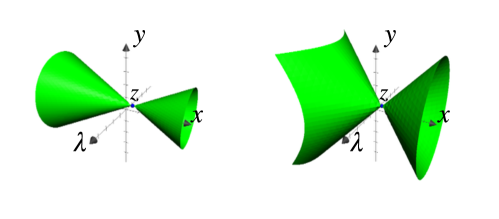
Figure 5: The stable cone $J_{u}(z,M)$ for $M=\frac{1}{2}$ on the left, and $M=1$ on the right.

The definition $W_{z}^{u}$ is related to cones, which is a nonstandard approach, the standard one is through convergence rates. In Theorem 9 we shall see that our definition implies the convergence rate as in the standard theory [12, 13].

Definition 18

We say that $F$ satisfies backward cone conditions if the following condition is fulfilled:

If $z_{1},z_{2},F(z_{1}),F(z_{2})\in D$ and $F(z_{1})\in J_{s}\left(F(z_{2}),1/L\right)$ then

$$z_{1}\in J_{s}\left(z_{2},1/L\right).$$

Intuitively, a function satisfies backward cone conditions, if images of two points are vertically aligned, then the points themselves are also vertically aligned. This is a technical condition that is associated with the fact that we do not assume invertibility of our map. In the setting of ODEs, the time shift along the trajectory map is invertible, and for small times it is close to identity. It will turn out that backward cone conditions are easily satisfied in the context of ODEs.

For $\lambda\in\Lambda$ we define the following sets:

$$D_{\lambda} =\overline{B}_{c}\left(\lambda,R_{\Lambda}\right)\times\overline{B}_{u}(R)\times\overline{B}_{s}(R),$$

$$D_{\lambda}^{+} =\overline{B}_{c}\left(\lambda,R_{\Lambda}\right)\times\overline{B}_{u}(R)\times\partial B_{s}(R),$$

$$D_{\lambda}^{-} =\overline{B}_{c}\left(\lambda,R_{\Lambda}\right)\times\partial\overline{B}_{u}(R)\times B_{s}(R).$$

Definition 19

We say that $F$ satisfies covering conditions if for any $z\in D$ there exists a $\lambda^{\ast}\in\Lambda$, such that the following conditions hold:

For $U=J_{u}(z,1/L)\cap D$, there exists a homotopy $h$

$$h:\left[0,1\right]\times U\rightarrow B_{c}\left(\lambda^{\ast},R_{\Lambda}\right)\times\mathbb{R}^{u}\times\mathbb{R}^{s},$$

and a linear map $A:\mathbb{R}^{u}\rightarrow\mathbb{R}^{u}$ which satisfy:

1. $h_{0}=F|_{U},$

2. for any $\alpha\in\left[0,1\right]$,

   $$h_{\alpha}\left(U\cap D_{\pi_{\theta}z}^{-}\right)\cap D_{\lambda^{\ast}} =\emptyset,$$ (46)

   $$h_{\alpha}\left(U\right)\cap D_{\lambda^{\ast}}^{+} =\emptyset,$$ (47)

3. $h_{1}\left(\lambda,x,y\right)=\left(\lambda^{\ast},Ax,0\right)$,

4. $A\left(\partial B_{u}(R)\right)\subset\mathbb{R}^{u}\setminus\overline{B}_{u}(R).$

In the above definition a reasonable choice for $\lambda^{\ast}$ will be $\lambda^{\ast}=\pi_{\lambda}F(z)$. In fact any point sufficiently close to $\pi_{\lambda}F(z)$ will be also good.

Intuitively, a function satisfies covering conditions if the coordinates are topologically correctly aligned with the dynamics. The $D^{+}_{\lambda}$ plays the role of the topological exit set, and $D^{-}_{\lambda}$ of topological entry.

4.2 Establishing center unstable manifolds for maps

In this section we present a theorem which can be used to establish existence of center unstable manifolds for maps.

Theorem 20

[6, Theorem 16 + Remark 62] Let $k\geq 1$ and $F:D\rightarrow\Lambda\times\mathbb{R}^{u}\times\mathbb{R}^{s}$ be a $C^{k+1}$ map. If $F$ satisfies covering conditions, rate conditions of order $k$ and backward cone conditions, then $W^{cu}$ is a $C^{k}$ manifold, which are graphs of a $C^{k}$ function

$$w^{cu}:\Lambda\times\overline{B}_{u}(R)\rightarrow\overline{B}_{s}(R),$$

meaning that

$$W^{cu}=\left\{\left(\lambda,x,w^{cu}(\lambda,y)\right):\lambda\in\Lambda,x\in\overline{B}_{u}(R)\right\}.$$

Moreover, $w^{cu}$ is Lipschitz with constant $L$.

The manifold $W^{cu}$ is foliated by invariant fibers $W_{z}^{u}$, which are graphs of $C^{k}$ functions

$$w_{z}^{u}:\overline{B}_{u}(R)\rightarrow\Lambda\times\overline{B}_{s}(R),$$

meaning that

$$W_{z}^{u}=\left\{\left(\pi_{\lambda}w_{z}^{u}\left(x\right),x,\pi_{y}w_{z}^{u}\left(x\right)\right):x\in\overline{B}_{u}(R)\right\}.$$

The functions $w_{z}^{u}$ are Lipschitz with constants $1/L$. Moreover, for $C=2R\left(1+1/L\right),$

$$W_{z}^{u} =\{p\in W^{cu}:\text{ }F^{-n}(p)\in D\text{ for all }n\in\mathbb{N}\text{,}$$ (48)

$$\left.\left\|F^{-n}\left(p\right)-F^{-n}\left(z\right)\right\|\leq C\xi_{u,1,P}^{-n}\text{ for all }n\in\mathbb{N}\right\}.$$

Observe that bound on $L\in\left(\frac{2R}{R_{\Lambda}},1\right)$ gives us lower bounds for the Lipschitz constants for functions $w^{cu}$, $w^{u}$, which is clearly an overestimate for the case when $\mathbb{T}\times\{0\}\times\{0\}$ is an invariant manifold. This lower bound is a consequence of choices we have made when formulating Theorem 20, as we did not want to introduce different constants for each type of cones, plus several inequalities between them. However, below theorem gives conditions which allow to obtain better Lipschitz constants.

Theorem 21

[6, Theorem 18] Let $M\in(0,1/L)$ and

$$\xi =\inf_{z\in D}m\left(\left[\frac{\partial F_{x}}{\partial x}(P(z))\right]\right)-M\sup_{z\in D}\left\|\frac{\partial F_{x}}{\partial\left(\lambda,y\right)}(z)\right\|,$$

$$\mu =\sup_{z\in D}\left\{\left\|\frac{\partial F_{\left(\lambda,y\right)}}{\partial\left(\lambda,y\right)}(z)\right\|+\frac{1}{M}\left\|\frac{\partial F_{\left(\lambda,y\right)}}{\partial x}(z)\right\|\right\}.$$

If assumptions of Theorem 20 hold true and also $\frac{\xi}{\mu}>1$, then the function $w_{z}^{u}$ from Theorem 20 is Lipschitz with constant $M.$

Theorem 22

[6, Theorem 19] Let $M\in(0,L)$ and

$$\xi =\inf_{z\in D}m\left[\frac{\partial F_{(\lambda,x)}}{\partial(\lambda,x)}(P(z))\right]-M\sup_{z\in D}\left\|\frac{\partial F_{(\lambda,x)}}{\partial y}(z)\right\|,$$

$$\mu =\sup_{z\in D}\left\{\left\|\frac{\partial F_{y}}{\partial y}\left(z\right)\right\|+\frac{1}{M}\left\|\frac{\partial F_{y}}{\partial(\lambda,x)}(z)\right\|\right\}.$$

If assumptions of Theorem 20 hold true and also $\frac{\xi}{\mu}>1$, then the function $w^{cu}$ from Theorem 20 is Lipschitz with constant $M$.

In our situation the map $F$ will be a time shift along a trajectory of an ODE, which is invertible. We can apply Theorem 20 to $F^{-1}$, (reversing the roles of coordinates $x,y$) and thus obtain the bounds for the center-stable manifold. The intersection of the center-stable manifold with the center-unstable manifold is the normally hyperbolic invariant manifold.

4.3 Dependence of manifolds on parameters

We consider a family of maps $F_{\varepsilon}:D\rightarrow\Lambda\times\mathbb{R}^{u}\times\mathbb{R}^{s}$ with $\varepsilon\in E$. For simplicity, we assume that $E=\mathbb{S}^{1}$. We can apply Theorem 20 to each of the maps separately and obtain a family of functions $w_{\varepsilon}^{cu}$ and $w_{z,\varepsilon}^{u}$ for $\varepsilon\in E$. We can also extend the map to include the parameter as follows. We first define $\tilde{\Lambda}=\mathbb{S}^{1}\times\Lambda$ and $\tilde{D}=\tilde{\Lambda}\times\overline{B}_{u}(R)\times\overline{B}_{s}(R)$ and consider

$$F:\tilde{D}\rightarrow\tilde{\Lambda}\times\mathbb{R}^{u}\times\mathbb{R}^{s},$$

defined as

$$F\left(\varepsilon,\lambda,x,y\right)=\left(\varepsilon,F_{\varepsilon}\left(\lambda,x,y\right)\right).$$

We can then apply Theorem 20 to $F$. This will establish existence of a center unstable manifold parameterized by

$$w^{cu}:\tilde{\Lambda}\times\overline{B}_{u}(R)\rightarrow\overline{B}_{s}(R).$$

Theorem 20 establishes that $w^{cu}$ is Lipschitz with constant $L$. This means that for any $\left(\lambda,x\right)\in\Lambda\times\overline{B}_{u}(R)$ and any $\varepsilon_{1},\varepsilon_{2}\in E$ we have

$$\left\|w_{\varepsilon_{1}}^{cu}\left(\lambda,x\right)-w_{\varepsilon_{2}}^{cu}\left(\lambda,x\right)\right\|=\left\|w^{cu}\left(\varepsilon_{1},\lambda,x\right)-w^{cu}\left(\varepsilon_{2},\lambda,x\right)\right\|\leq L\left\|\varepsilon_{1}-\varepsilon_{2}\right\|.$$

If assumptions of Theorem 20 are applied with $k>1$, then we know that $w^{cu}$ is $C^{1}$, and above inequality gives us the following dependence with respect to the parameter

$$\left\|\frac{\partial}{\partial\varepsilon}w_{\varepsilon}^{cu}\left(\lambda,x\right)\right\|\leq L.$$

Extending the $\Lambda$ to include the parameter can also be used to establish bounds on the second or mixed derivative of $w_{\varepsilon}^{cu}$ with respect to the parameter, by using the method given in section 4.4 below.

4.4 Bounds on second derivatives

In this section we shall show how we can obtain explicit bounds on the second derivatives of the parameterization of the center unstable manifold established in Theorem 20.

For the sake of simplicity, we shall use two coordinates $\mathrm{x}$ and $\mathrm{y}$. We shall study the bounds on the second derivative of a function $\mathrm{y}=w\left(\mathrm{x}\right)$ under appropriate rate conditions. In applications, we can have:

• $\mathrm{x}=x,$ $\mathrm{y}=\left(\lambda,y\right)$ and $w(\mathrm{x})=w_{z}^{u}\left(\mathrm{x}\right)$;

• $\mathrm{x}=\left(\lambda,x\right),$ $\mathrm{y}=y$ and $w(\mathrm{x})=w^{cu}\left(\mathrm{x}\right).$

Similarly, in the case of a family of maps, which depend on parameters (as discussed in Section 4.3), we can have:

• $\mathrm{x}=x,$ $\mathrm{y}=\left(\varepsilon,\lambda,y\right)$ and $w(\mathrm{x})=w_{z}^{u}\left(\mathrm{x}\right)$;

• $\mathrm{x}=\left(\varepsilon,\lambda,x\right),$ $\mathrm{y}=y$ and $w(\mathrm{x})=w^{cu}\left(\mathrm{x}\right).$

We shall assume that $(\mathrm{x},\mathrm{y})\in\mathbb{R}^{u+s}$ and consider $F:D\rightarrow\mathbb{R}^{u+s}$ which is $C^{3}$ differentiable, where $D\subset\mathbb{R}^{u+s}$ is the domain of $F$.

We assume that $F$ is such that if $v:\mathbb{R}^{u}\rightarrow\mathbb{R}^{s}$ is Lipschitz with constant $\mathcal{L}>0$, then the graph transform $\mathcal{G}\left(v\right)$ is well defined i.e.

$$\mathcal{G}\left(v\right)=F_{y}\circ\left(\mathrm{id},v\right)\circ\left(F_{x}\circ\left(\mathrm{id},v\right)\right)^{-1}.$$ (49)

Assume also that for $v_{0}\left(\mathrm{x}\right)=0$

$$w=\lim_{n\rightarrow\infty}\mathcal{G}^{n}\left(v_{0}\right).$$ (50)

Such is the setting in the construction of $w=w^{cu}$ and $w=w_{z}^{u}$ in [6]. In such case, the property (50) follows from assumptions of Theorem 20; see [6, Lemma 46] and [6, Lemma 57]. In the case of $w=w^{cu}$ we take $\mathcal{L}=L$ (where $L$ is the constant from Theorem 20) and for $w=w_{z}^{u}$ we take $\mathcal{L}=1/L$. The following result will allow us to obtain estimates on the second derivative of $w$.

Theorem 23

Let $\mathcal{L}>0$ and define

$$\xi =\inf_{z\in D}\left(m\left(\frac{\partial F_{\mathrm{x}}}{\partial\mathrm{x}}(z)\right)-\mathcal{L}\left\|\frac{\partial F_{\mathrm{x}}}{\partial\mathrm{y}}(z)\right\|\right),$$

$$\mu_{1} =\sup_{z\in D}\left(\left\|\frac{\partial F_{\mathrm{y}}}{\partial\mathrm{y}}(z)\right\|+\frac{1}{\mathcal{L}}\left\|\frac{\partial F_{\mathrm{y}}}{\partial\mathrm{x}}(z)\right\|\right),$$

$$\mu_{2} =\sup_{z\in D}\left(\left\|\frac{\partial F_{\mathrm{y}}}{\partial\mathrm{y}}(z)\right\|+\mathcal{L}\left\|\frac{\partial F_{\mathrm{x}}}{\partial\mathrm{y}}(z)\right\|\right).$$

Assume that

$$\xi>0,\qquad\frac{\mu_{1}}{\xi}<1,\qquad\frac{\mu_{2}}{\xi^{2}}<1.$$ (51)

Let

$$C_{x} =\frac{1}{2}\max_{p\in D,\|h\|=1}\|D^{2}F_{\mathrm{x}}(p)(h,h)\|,$$ (52)

$$C_{y} =\frac{1}{2}\max_{p\in D,\|h\|=1}\|D^{2}F_{\mathrm{y}}(p)(h,h)\|.$$ (53)

and

$$C_{y,1} =\sup_{p\in D}\frac{1}{2}\left\|\frac{\partial^{2}F_{\mathrm{y}}}{\partial\mathrm{x}^{2}}(p)\right\|,$$

$$C_{y,2} =\sup_{p\in D}\left\|\frac{\partial^{2}F_{\mathrm{y}}}{\partial\mathrm{x}\partial\mathrm{y}}(p)\right\|,$$ (54)

$$C_{y,3} =\sup_{p\in D}\frac{1}{2}\left\|\frac{\partial^{2}F_{\mathrm{y}}}{\partial\mathrm{y}^{2}}(p)\right\|.$$

Then for any $\mathrm{x}$ and $h$ holds (where it makes sense) where $w$ is defined by (50)

$$w(\mathrm{x}+h)=w(\mathrm{x})+Dw(\mathrm{x})h+\Delta y(\mathrm{x},h),\quad\|\Delta y(\mathrm{x},h)\|\leq M\|h\|^{2}$$ (55)

where

$$M>\frac{(\mathcal{L}C_{x}+C_{y})(1+\mathcal{L}^{2})}{\xi^{2}-\mu_{2}}.$$ (56)

One can obtain an alternative (giving tighter estimates; see Remark 24) expression for $M$

$$M>\frac{\mathcal{L}C_{x}(1+\mathcal{L}^{2})+C_{y,1}+C_{y,2}\mathcal{L}+C_{y,3}\mathcal{L}^{2}}{\xi^{2}-\mu_{2}}$$ (57)

Hence for any $h\in\mathbb{R}^{u}$ holds

$$\left\|\frac{1}{2}D^{2}w\left(\mathrm{x}\right)(h,h)\right\|\leq M\|h\|^{2}.$$

Proof. For a $s\times u$ matrix $A$, $M\in\mathbb{R},$ and a point $z\in\mathbb{R}^{u+s}$ we define a set (see Figure 6)

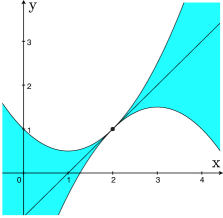
Figure 6: The set $J_{u}(z,A,M)$ for $z=\left(2,1\right)$, $A=1$ and $M=\frac{1}{2}$, in blue.

$$J_{u}(z,A,M)=\{z+(\mathrm{x},A\mathrm{x}+\mathrm{y}):\quad\|\mathrm{y}\|\leq M\|\mathrm{x}\|^{2}\}.$$ (58)

We shall look for the smallest $M$, such that for all $z\in D$ and all $\|A_{0}\|\leq\mathcal{L}$ there exists a $A_{1}$ such that $\|A_{1}\|\leq\mathcal{L}$ and

$$F(J_{u}(z,A_{0},M))\cap B(0,\delta))\subset J_{u}(F(z),A_{1},M),$$ (59)

for sufficiently small $\delta>0$ (which might depend on $z$ and $A_{0}$).

From now on we assume that $\|A_{0}\|\leq\mathcal{L}$.

Let us set

$$D_{\mathrm{x}} =\frac{\partial F_{\mathrm{x}}}{\partial\mathrm{x}}(z)+\frac{\partial F_{\mathrm{x}}}{\partial\mathrm{y}}(z)A_{0},$$

$$D_{\mathrm{y}} =\frac{\partial F_{\mathrm{y}}}{\partial\mathrm{x}}(z)+\frac{\partial F_{\mathrm{y}}}{\partial\mathrm{y}}(z)A_{0}.$$

Observe that by the definition of $\xi$

$$m(D_{\mathrm{x}})\geq m\left(\frac{\partial F_{\mathrm{x}}}{\partial\mathrm{x}}(z)\right)-\left\|\frac{\partial F_{\mathrm{x}}}{\partial\mathrm{y}}(z)\right\|\left\|A_{0}\right\|\geq\xi>0.$$ (60)

We take

$$A_{1}=D_{\mathrm{y}}D_{\mathrm{x}}^{-1}.$$

From (51) follows that if $\|A_{0}\|\leq\mathcal{L}$, then

$$\left\|A_{1}\right\|=\left\|D_{\mathrm{y}}D_{\mathrm{x}}^{-1}\right\|\leq\frac{\left\|\frac{\partial F_{\mathrm{y}}}{\partial\mathrm{x}}(z)\right\|+\left\|\frac{\partial F_{\mathrm{y}}}{\partial\mathrm{y}}(z)\right\|\left\|A_{0}\right\|}{m\left(\frac{\partial F_{\mathrm{x}}}{\partial\mathrm{x}}(z)\right)-\left\|\frac{\partial F_{\mathrm{x}}}{\partial\mathrm{y}}(z)\right\|\left\|A_{0}\right\|}\leq\frac{\mathcal{L}\mu_{1}}{\xi}<\mathcal{L}.$$ (61)

Let $h=\left(\mathrm{x},A_{0}\mathrm{x}+\mathrm{y}\right)$. For $z+h\in J_{u}(z,A,M)$, by (58), we have

$$\|A_{0}\mathrm{x}+\mathrm{y}\|\leq\|A_{0}\|\|\mathrm{x}\|+M\|\mathrm{x}\|^{2}\leq\|\mathrm{x}\|\left(\mathcal{L}+M\|\mathrm{x}\|\right).$$

Let $(\mathrm{x}_{1},\mathrm{\tilde{y}})=F(z+h)-F(z)$ and let $\mathrm{y}_{1}=\mathrm{\tilde{y}}-A_{1}\mathrm{x}_{1}$. Note that

$$F(z+h)=F(z)+\left(\mathrm{x}_{1},A_{1}\mathrm{x}_{1}+\mathrm{y}_{1}\right).$$

Our goal will be to find a bound on $\frac{\|\mathrm{y}_{1}\|}{\|\mathrm{x}_{1}\|^{2}}$, and to show that $\frac{\|\mathrm{y}_{1}\|}{\|\mathrm{x}_{1}\|^{2}}\leq M.$ First we need to establish a number of estimates.

We have

$$\mathrm{x}_{1} =F_{\mathrm{x}}(z+h)-F_{\mathrm{x}}(z)$$

$$=\frac{\partial F_{\mathrm{x}}}{\partial\mathrm{x}}(z)\mathrm{x}+\frac{\partial F_{\mathrm{x}}}{\partial\mathrm{y}}(z)\left(A_{0}\mathrm{x}+\mathrm{y}\right)+R_{\mathrm{x},2}\left(z,h\right)$$

$$=D_{\mathrm{x}}\mathrm{x}+\frac{\partial F_{\mathrm{x}}}{\partial\mathrm{y}}(z)\mathrm{y}+R_{\mathrm{x},2}\left(z,h\right).$$ (62)

From (52) we know that

$$\left\|R_{\mathrm{x},2}\left(z,h\right)\right\|\leq C_{x}\left\|h\right\|^{2}\leq C_{x}\left(\left\|\mathrm{x}\right\|^{2}+\left\|A_{0}\mathrm{x}+\mathrm{y}\right\|^{2}\right)\leq R_{x}\|\mathrm{x}\|^{2},$$ (63)

where

$$R_{x}\leq C_{x}(1+(\mathcal{L}+M\|\mathrm{x}\|)^{2}).$$

Thus

$$\left\|\mathrm{x}_{1}-\left(D_{\mathrm{x}}\mathrm{x}+\frac{\partial F_{\mathrm{x}}}{\partial\mathrm{y}}(z)\mathrm{y}\right)\right\|\leq R_{x}\|\mathrm{x}\|^{2}.$$

Using mirror computations, for $\mathrm{\tilde{y}}$ from (53) we obtain

$$\left\|\mathrm{\tilde{y}}-\left(D_{\mathrm{y}}\mathrm{x}+\frac{\partial F_{\mathrm{y}}}{\partial\mathrm{y}}(z)\mathrm{y}\right)\right\|\leq R_{y}\|\mathrm{x}\|^{2},$$

with

$$R_{y}\leq C_{y}\left(1+(\mathcal{L}+M\|\mathrm{x}\|)^{2}\right).$$ (64)

We have another possible variants for $R_{y}$ based on (54). We can compute

$$\mathrm{\tilde{y}}=D_{\mathrm{y}}\mathrm{x}+\frac{\partial F_{\mathrm{y}}}{\partial\mathrm{y}}(z)\mathrm{y}+R_{\mathrm{y},2}\left(z,h\right),$$ (65)

with the estimate

$$\left\|R_{\mathrm{y},2}\left(z,h\right)\right\| \leq\sup_{p\in D}\frac{1}{2}\left\|\frac{\partial^{2}F_{\mathrm{y}}}{\partial\mathrm{x}^{2}}(p)\right\|\left\|\mathrm{x}\right\|^{2}+\sup_{p\in D}\left\|\frac{\partial^{2}F_{\mathrm{y}}}{\partial\mathrm{x}\partial\mathrm{y}}(p)\right\|\left\|\mathrm{x}\right\|\left\|\mathrm{y}\right\|$$

$$+\sup_{p\in D}\frac{1}{2}\left\|\frac{\partial^{2}F_{\mathrm{y}}}{\partial\mathrm{y}^{2}}(p)\right\|\left\|\mathrm{y}\right\|^{2}$$

$$\leq C_{y,1}\left\|\mathrm{x}\right\|^{2}+C_{y,2}\left\|\mathrm{x}\right\|\left\|A_{0}\mathrm{x}+\mathrm{y}\right\|+C_{y,3}\left\|A_{0}\mathrm{x}+\mathrm{y}\right\|$$

$$\leq\left\|\mathrm{x}\right\|^{2}R_{y}^{(2)},$$

for

$$R_{y}^{(2)}\leq C_{y,1}+C_{y,2}(\mathcal{L}+M\|\mathrm{x}\|)+C_{y,3}(\mathcal{L}+M\|\mathrm{x}\|)^{2}.$$ (66)

To compute the bound for $\frac{\|\mathrm{y}_{1}\|}{\|\mathrm{x}_{1}\|^{2}}$ we must ensure that $\left\|\mathrm{x}_{1}\right\|\neq 0$. From (62) and (63)

$$\|\mathrm{x}_{1}\|\geq\|\mathrm{x}\|\left(m(D_{x})-\left\|\frac{\partial F_{\mathrm{x}}}{\partial\mathrm{y}}\right\|M\|\mathrm{x}\|-R_{x}\|\mathrm{x}\|\right).$$ (67)

Since by (60) $m(D_{x})>0,$ we thus see that for sufficiently small $\left\|\mathrm{x}\right\|$ (how small may depend on $M$) we shall have $\|\mathrm{x}_{1}\|>0.$

From (62) we have

$$\mathrm{x}=D_{\mathrm{x}}^{-1}\mathrm{x}_{1}-D_{\mathrm{x}}^{-1}\frac{\partial F_{\mathrm{x}}}{\partial\mathrm{y}}(z)\mathrm{y}-D_{\mathrm{x}}^{-1}R_{\mathrm{x},2}\left(z,h\right)$$

hence by (65)

$$\mathrm{\tilde{y}} =D_{\mathrm{y}}\left(D_{\mathrm{x}}^{-1}\mathrm{x}_{1}-D_{\mathrm{x}}^{-1}\frac{\partial F_{\mathrm{x}}}{\partial\mathrm{y}}(z)\mathrm{y}-D_{\mathrm{x}}^{-1}R_{\mathrm{x},2}\left(z,h\right)\right)$$

$$+\frac{\partial F_{\mathrm{y}}}{\partial\mathrm{y}}(z)\mathrm{y}+R_{\mathrm{y},2}\left(z,h\right)$$

$$=A_{1}x_{1}+\left(-A_{1}\frac{\partial F_{\mathrm{x}}}{\partial\mathrm{y}}(z)+\frac{\partial F_{\mathrm{y}}}{\partial\mathrm{y}}(z)\right)\mathrm{y}$$

$$-A_{1}R_{\mathrm{x},2}\left(z,h\right)+R_{\mathrm{y},2}\left(z,h\right)$$

which by (61) and (63) gives

$$\left\|\mathrm{y}_{1}\right\| =\left\|\mathrm{\tilde{y}}-A_{1}\mathrm{x}_{1}\right\|$$ (68)

$$\leq\left\|\left(-A_{1}\frac{\partial F_{\mathrm{x}}}{\partial\mathrm{y}}(z)+\frac{\partial F_{\mathrm{y}}}{\partial\mathrm{y}}(z)\right)\mathrm{y}\right\|$$

$$+\|A_{1}\|R_{x}\|\mathrm{x}\|^{2}+R_{y}\|\mathrm{x}\|^{2}$$

$$\leq\mu_{2}\left\|\mathrm{y}\right\|+\mathcal{L}R_{x}\|\mathrm{x}\|^{2}+R_{y}\|\mathrm{x}\|^{2}$$

$$\leq\left\|\mathrm{x}\right\|^{2}\left(\mu_{2}M+\mathcal{L}R_{x}+R_{y}\right).$$

Since by (60) $m(D_{\mathrm{x}})>\xi$ by combining (67) and (68) we obtain

$$\frac{\|y_{1}\|}{\|x_{1}\|^{2}} \leq\frac{\left\|\mathrm{x}\right\|^{2}\left(\mu_{2}M+\mathcal{L}R_{x}+R_{y}\right)}{\|\mathrm{x}\|^{2}\left(\xi-\left\|\frac{\partial F_{\mathrm{x}}}{\partial\mathrm{y}}\right\|M\|\mathrm{x}\|-R_{x}\|\mathrm{x}\|\right)^{2}}$$

$$=M\frac{\frac{\mu_{2}}{\xi^{2}}+\frac{1}{\xi^{2}M}\left(\mathcal{L}R_{x}+R_{y}\right)}{\left(1-\frac{\|\mathrm{x}\|}{\xi}\left(\left\|\frac{\partial F_{\mathrm{x}}}{\partial\mathrm{y}}\right\|M+R_{x}\right)\right)^{2}}.$$

We want this ratio to be less than $M$ for sufficiently small $\|x\|$. Therefore we can set $\|x\|=0$, so we obtain the following condition

$$\frac{\mu_{2}}{\xi^{2}}+\frac{1}{\xi^{2}M}\left(\mathcal{L}R_{x}+R_{y}\right)<1.$$

This condition follows from (56) for $R_{y}$ given by (64). For $R_{y}=R_{y}^{(2)}$, where $R_{y}^{(2)}$ was defined in (66), above condition follows from (57).

By our assumption (50), we know that $w=\lim_{n\rightarrow+\infty}\mathcal{G}^{n}\left(v_{0}\right)$. Taking $A_{0}=0$ we see that for any $z\in\mathrm{graph}\left(v_{0}\right)$ and for sufficiently small $\delta$

$$\mathrm{graph}\left(v_{0}\right)\cap B\left(z,\delta\right)\subset J_{u}\left(z,A_{0},M\right).$$

By (59),

$$\mathrm{graph}\left(\mathcal{G}\left(v_{0}\right)\right)\cap B\left(z,\delta\right)\subset J_{u}\left(F(z),A_{1},M\right).$$

Applying this argument inductively, for any $z\in\mathrm{graph}\left(w\right),$ taking $A=Dw\left(z\right)$,

$$\mathrm{graph}\left(w\right)\cap B\left(z,\delta\right)\subset J_{u}\left(z,A,M\right).$$ (69)

From (69) follows (55), which concludes our proof.   

Remark 24

Observe that in the case of totally flat invariant manifold $($$x$$,0)$ we have $F_{\mathrm{y}}(\mathrm{x},\mathrm{y})=g(\mathrm{x},\mathrm{y})\mathrm{y}$ and $\mathcal{L}$ could be taken as small as we want.

In such case we obtain from (56) the bound $M\approx\frac{C_{\mathrm{y}}}{\xi^{2}-\mu}$, which might be quite large as $C_{\mathrm{y}}$ depends on $\frac{\partial^{2}F_{\mathrm{y}}}{\partial\mathrm{x}\partial\mathrm{y}}$ and $\frac{\partial^{2}F_{\mathrm{y}}}{\partial\mathrm{y}^{2}},$ which might be nonzero even on our flat manifold.

When using (57) we obtain $M\approx\frac{C_{\mathrm{y},1}}{\xi^{2}-\mu}$, where $C_{\mathrm{y},1}$ is to be expected to be very small, because $D_{\mathrm{x}}^{2}F_{\mathrm{y}}(\mathrm{x},\mathrm{y})=(D_{\mathrm{x}}^{2}g(\mathrm{x},\mathrm{y}))\mathrm{y}$, hence it vanishes on the invariant manifold.

Using Theorem 23 we can obtain estimates on the partial derivatives of $w$ using the following lemma.

Lemma 25

Assume that $\|D^{2}w\left(\mathrm{x}\right)(h,h)\|\leq 2M\|h\|^{2}$. Then in orthogonal coordinates $(\mathrm{x}_{1},\dots,\mathrm{x}_{n})$ holds

$$\left\|\frac{\partial^{2}w}{\partial\mathrm{x}_{i}\partial\mathrm{x}_{j}}\right\|\leq 2M,\quad i,j=1,\dots,n.$$

Proof. Let us denote by $W$ the symmetric map $D^{2}w$. Let $e_{1},\dots,e_{n}$ be a basis corresponding our coordinates. Then

$$W(e_{i},e_{j})=\frac{\partial^{2}F}{\partial\mathrm{x}_{i}\partial\mathrm{x}_{j}}.$$

Our task is to recover the map $W$ knowing only the behavior on the diagonal. This is accomplished using the following identity

$$W(p+q,p+q)-W(p-q,p-q)=4W(p,q).$$

Let us set $p=e_{i}+e_{j}$ and $q=e_{i}-e_{j}$. Observe that $\|p\|^{2}=\|q\|^{2}=2$. We have

$$4\left\|W(e_{i},e_{j})\right\| \leq\left\|W(e_{i}+e_{j},e_{i}+e_{j})\right\|+\left\|W(e_{i}-e_{j},e_{i}-e_{j})\right\|$$

$$\leq 2\cdot 2M\sqrt{2}^{2},$$

which concludes our proof.   

5 Center-unstable manifolds for ODEs

In this section we show how to establish the existence of center unstable manifolds for ODEs. The results will follow from the ones established for maps in section 4. To obtain our results, we will consider the time shift map along the solution of the ODE. Our objective though will be to reformulate the conditions to obtain our results based on assumptions on the vector field, rather than to integrate the ODE.

5.1 Definitions and setup

We consider an ODE

$$q^{\prime}=f(q)$$ (70)

where

$$f:\Lambda\times\mathbb{R}^{u}\times\mathbb{R}^{s}\rightarrow\mathbb{R}^{c}\times\mathbb{R}^{u}\times\mathbb{R}^{s}.$$

We denote by $\Phi\left(t,q\right)$ the flow induced by (70).

We shall consider a set

$$D=\Lambda\times\overline{B}_{u}\left(R\right)\times\overline{B}_{s}\left(R\right).$$

Definition 26

We define the center-unstable set of (70) in $D$ as

$$W_{\mathrm{loc},D}^{cu}=\{z:\Phi\left(t,z\right)\in D\text{ for all }t<0\}.$$

Since the set $D$ will remain fixed throughout the discussion, from now on we will simplify notation by writing $W^{cu}$ instead of $W_{\mathrm{loc},D}^{cu}.$

As in section 4.1, we consider a constant $L\in\left(\frac{2R}{R_{\Lambda}},1\right),$ and define the stable fiber analogously to Definition 17.

Definition 27

Assume that $z\in W^{cu}$. We define the unstable fiber of $z$ as

$$W_{z}^{u}=\{p\in D:\Phi\left(t,p\right)\in J_{u}\left(\Phi\left(t,z\right),1/L\right)\cap D,\text{ for all }t<0\}.$$

Let us introduce the following constants (compare with constants from section 4.1 for maps)

$$\overrightarrow{\mu_{s,1}} =\sup_{z\in D}\left\{l\left(\frac{\partial f_{y}}{\partial y}(z)\right)+\frac{1}{L}\left\|\frac{\partial f_{y}}{\partial(\lambda,x)}(z)\right\|\right\},$$

$$\overrightarrow{\mu_{s,2}} =\sup_{z\in D}\left\{l\left(\frac{\partial f_{y}}{\partial y}\left(z\right)\right)+L\left\|\frac{\partial f_{\left(\lambda,x\right)}}{\partial y}(z)\right\|\right\},$$

$$\overrightarrow{\xi_{u,1}} =\inf_{z\in D}\left\{m_{l}\left(\frac{\partial f_{x}}{\partial x}(z)\right)-\frac{1}{L}\left\|\frac{\partial f_{x}}{\partial\left(\lambda,y\right)}(z)\right\|\right\},$$

$$\overrightarrow{\xi_{u,1,P}} =\inf_{z\in D}m_{l}\left(\frac{\partial f_{x}}{\partial x}(P(z))\right)-\frac{1}{L}\sup_{z\in D}\left\|\frac{\partial f_{x}}{\partial\left(\lambda,y\right)}(z)\right\|,$$

$$\overrightarrow{\mu_{cs,1}} =\sup_{z\in D}\left\{l\left(\frac{\partial f_{\left(\lambda,y\right)}}{\partial\left(\lambda,y\right)}(z)\right)+L\left\|\frac{\partial f_{\left(\lambda,y\right)}}{\partial x}(z)\right\|\right\},$$

$$\overrightarrow{\mu_{cs,2}} =\sup_{z\in D}\left\{l\left(\frac{\partial f_{\left(\lambda,y\right)}}{\partial\left(\lambda,y\right)}(z)\right)+\frac{1}{L}\left\|\frac{\partial f_{x}}{\partial\left(\lambda,y\right)}(z)\right\|\right\},$$

$$\overrightarrow{\xi_{cu,1}} =\inf_{z\in D}\left\{m_{l}\left(\frac{\partial f_{(\lambda,x)}}{\partial(\lambda,x)}(z)\right)-L\left\|\frac{\partial f_{(\lambda,x)}}{\partial y}(z)\right\|\right\},$$

$$\overrightarrow{\xi_{cu,1,P}} =\inf_{z\in D}m_{l}\left(\frac{\partial f_{(\lambda,x)}}{\partial(\lambda,x)}(P(z))\right)-L\sup_{z\in D}\left\|\frac{\partial f_{(\lambda,x)}}{\partial y}(z)\right\|.$$

The arrow is used to emphasize that the constants are computed for the vector field.

Analogously to the case of maps (Definition 14) we define the rate conditions for ODEs as follows.

Definition 28

We say that the vector field $f$ satisfies rate conditions of order $k\geq 1$ if for all $k\geq j\geq 1$ holds

$$\overrightarrow{\mu_{s,1}}<0<\overrightarrow{\xi_{u,1,P}},$$ (71)

$$\overrightarrow{\mu_{cs,1}}<\overrightarrow{\xi_{u,1,P}},\qquad\qquad\overrightarrow{\mu_{s,1}}<\overrightarrow{\xi_{cu,1,P}},$$ (72)

$$\overrightarrow{\mu_{s,2}}<\left(j+1\right)\overrightarrow{\xi_{cu,1}},\qquad\overrightarrow{\mu_{cs,2}}<\overrightarrow{\xi_{u,1}}.$$ (73)

We now define the notion of an isolating block.

Definition 29

We say that $D=\Lambda\times\overline{B}_{u}\left(R\right)\times\overline{B}_{s}\left(R\right)$ is an isolating block for (70) if

1. For any $q\in\Lambda\times\partial\overline{B}_{u}\left(R\right)\times\overline{B}_{s}\left(R\right)$,

   $$\left(\pi_{x}f(q)|\pi_{x}q\right)>0.$$

2. For any $q\in\Lambda\times\overline{B}_{u}\left(R\right)\times\partial\overline{B}_{s}\left(R\right)$,

   $$\left(\pi_{y}f(q)|\pi_{y}q\right)<0.$$

Isolating blocks are important constructs in the Conley index theory [23]. Intuitively, in Definition 29 the set $\Lambda\times\partial\overline{B}_{u}\left(R\right)\times\overline{B}_{s}\left(R\right)$ plays the role of the exit set, and $\Lambda\times\overline{B}_{u}\left(R\right)\times\partial\overline{B}_{s}\left(R\right)$ of the entry set. Isolating blocks will play the same role as the covering condition for maps (Definition 19).

Theorem 30

Let $k\geq 1$. Assume that $f$ is $C^{k+1}$ and satisfies rate conditions of order $k$. Assume also that $D=\Lambda\times\overline{B}_{u}\left(R\right)\times\overline{B}_{s}\left(R\right)$ is an isolating segment for $f$. Then the center-unstable set $W^{cu}$ in $D$ is a $C^{k}$ manifold, which satisfies the properties listed in Theorem 20.

The manifold $W^{cu}$ is foliated by invariant fibers $W_{z}^{u}$, which are graphs of $C^{k}$ functions (as in Theorem 20). Moreover, for $C=2R\left(1+1/L\right),$

$$W_{z}^{u} = \{p\in W^{cu}:\text{ }\Phi\left(-t,p\right)\in D\text{ for all }t>0\text{,}$$

$$\left.\left\|\Phi\left(-t,p\right)-\Phi\left(-t,z\right)\right\|\leq Ce^{-t\overrightarrow{\xi_{u,1,P}}}\text{ for all }t>0\right\}.$$

Proof. The proof is given in section 5.5.   

The proof of Theorem 30 will follow from Theorem 20, applied to a time shift along the trajectory. In section 5.2 we will show how rate conditions (for maps; as in Definition 14) follow from Definition 28 for the time shift map along the trajectory. In section 28 we will show how the covering condition (Definition 19) follows from Definition 29. This will lead to the proof of Theorem 30 in section 5.5.

5.2 Verification of rate conditions

We consider an ODE

$$z^{\prime}=f\left(z\right),$$ (75)

where $z=\left(x,y\right)$ and $f=\left(f_{x},f_{y}\right)$. Consider a shift by $h>0$ along the solution of (75), which we will denote by $\Phi(h,z)=\left(\Phi_{x}(h,z),\Phi_{y}(h,z)\right)$. We will show how to establish rate conditions for a map $F\left(z\right)=\Phi(h,z)$, for sufficiently small (fixed) $h.$

The results obtained in this section will be applicable for the setting where:

• $\mathrm{x}=x,$ $\mathrm{y}=\left(\lambda,y\right),$

• $\mathrm{x}=\left(\lambda,x\right),$ $\mathrm{y}=y,$

Similarly, in the case of a family of maps (as discussed in Section 4.3), which depend on parameters, we can have:

• $\mathrm{x}=x,$ $\mathrm{y}=\left(\varepsilon,\lambda,y\right)$,

• $\mathrm{x}=\left(\varepsilon,\lambda,x\right),$ $\mathrm{y}=y$.

We define

$$\overrightarrow{\xi\left(M\right)} = \inf_{z\in D}\left\{m_{l}\left(\frac{\partial f_{\mathrm{x}}}{\partial\mathrm{x}}(z)\right)-M\left\|\frac{\partial f_{\mathrm{x}}}{\partial\mathrm{y}}(z)\right\|\right\},$$

$$\overrightarrow{\xi_{P}\left(M\right)} = \inf_{z\in D}m_{l}\left(\frac{\partial f_{\mathrm{x}}}{\partial\mathrm{x}}(P(z))\right)-M\sup_{z\in D}\left\|\frac{\partial f_{\mathrm{x}}}{\partial\mathrm{y}}(z)\right\|,$$

$$\overrightarrow{\mu_{1}(M)} = \sup_{z\in D}\left\{l\left(\frac{\partial f_{\mathrm{y}}}{\partial\mathrm{y}}(z)\right)+M\left\|\frac{\partial f_{\mathrm{y}}}{\partial\mathrm{x}}(z)\right\|\right\},$$

$$\overrightarrow{\mu_{2}(M)} = \sup_{z\in D}\left\{l\left(\frac{\partial f_{\mathrm{y}}}{\partial\mathrm{y}}(h,z)\right)+M\left\|\frac{\partial f_{\mathrm{x}}}{\partial\mathrm{y}}(h,z)\right\|\right\}.$$

We also consider the following quantities, which are defined for a given $h>0$

$$\xi(h,M) = \inf_{z\in D}\left\{m\left(\frac{\partial\Phi_{\mathrm{x}}}{\partial\mathrm{x}}(h,z)\right)-M\left\|\frac{\partial\Phi_{\mathrm{x}}}{\partial\mathrm{y}}(h,z)\right\|\right\},$$

$$\xi_{P}\left(h,M\right) = \inf_{z\in D}m\left(\frac{\partial\Phi_{\mathrm{x}}}{\partial\mathrm{x}}(h,P(z))\right)-M\sup_{z\in D}\left\|\frac{\partial\Phi_{\mathrm{x}}}{\partial\mathrm{y}}(h,z)\right\|,$$

$$\mu_{1}(h,M) = \sup_{z\in D}\left\{\left\|\frac{\partial\Phi_{\mathrm{y}}}{\partial\mathrm{y}}(h,z)\right\|+M\left\|\frac{\partial\Phi_{\mathrm{y}}}{\partial\mathrm{x}}(h,z)\right\|\right\},$$

$$\mu_{2}(h,M) = \sup_{z\in D}\left\{\left\|\frac{\partial\Phi_{\mathrm{y}}}{\partial\mathrm{y}}(h,z)\right\|+M\left\|\frac{\partial\Phi_{\mathrm{x}}}{\partial\mathrm{y}}(h,z)\right\|\right\}.$$

(in the application we will choose $M$ as $L$ or $1/L$, depending on which of the rate conditions (43–45) we wish to verify).

Below theorem can be used to establish the fact that rate conditions (see Definition 14) hold for the time shift map $\Phi(h,\cdot)$.

Theorem 31

Let $M,M_{1},M_{2}>0$. We have the following conditions:

1. We have

   $$\xi(h,M) = 1+h\overrightarrow{\xi(M)}+O(h^{2})$$ (76)

   $$\xi_{P}\left(h,M\right) = 1+h\overrightarrow{\xi_{P}\left(M\right)}+O(h^{2}),$$ (77)

   $$\mu_{1}(h,M) = 1+h\overrightarrow{\mu_{1}(M)}+O(h^{2}),$$ (78)

   $$\mu_{2}(h,M) = 1+h\overrightarrow{\mu_{2}(M)}+O(h^{2}).$$ (79)

2. If for $j\geq 0$

   $$\overrightarrow{\mu_{2}(M_{1})}<\left(j+1\right)\overrightarrow{\xi\left(M_{2}\right)},$$ (80)

   then for sufficiently small $h_{0}>0$, and for any $h\in\left(0,h_{0}\right)$,

   $$\frac{\mu_{2}(h,M_{1})}{\xi(h,M_{2})^{j+1}}<1.$$

3. If $\overrightarrow{\mu_{1}(M_{1})}<\overrightarrow{\xi_{P}\left(M_{2}\right)}$ then for sufficiently small $h_{0}>0$, and for any $h\in\left(0,h_{0}\right)$,

   $$\frac{\mu_{1}(h,M_{1})}{\xi_{P}(h,M_{2})}<1.$$

4. If $\overrightarrow{\xi_{P}\left(M\right)}>0$ then for sufficiently small $h_{0}>0$, and for any $h\in\left(0,h_{0}\right)$,

   $$\xi_{P}\left(h,M\right)>1.$$

   Also

   $$\xi_{P}\left(h,M\right)=1+h\overrightarrow{\xi_{P}\left(M\right)}+O(h^{2}).$$

5. If $\overrightarrow{\mu_{1}(M)}<0$ then for sufficiently small $h_{0}>0$, and for any $h\in\left(0,h_{0}\right)$,

   $$\mu_{1}(h,M)<1.$$

6. If $h_{0}>0$ is sufficiently small, then for any $h\in\left(0,h_{0}\right)$,

   $$\xi_{P}\left(h,M\right)>0\qquad\text{and\qquad}\xi\left(h,M\right)>0.$$

Proof. We have

$$\Phi(h,z) = z+hf(z)+O(h^{2})$$

$$\frac{\partial\Phi}{\partial z}(h,z) = I+hDf(z)+O(h^{2}),$$

$$D_{z}^{2}\Phi(h,z) = hD^{2}f(z)+O(h^{2}).$$ (81)

where the $O(h^{2})$ are uniform in $z$ for $z\in D$.

Using (7) and Lemma 8 we obtain

$$m\left(\frac{\partial\Phi_{\mathrm{x}}}{\partial\mathrm{x}}(h,z)\right) = m\left(I+h\frac{\partial f_{\mathrm{x}}}{\partial\mathrm{x}}+O(h^{2})\right)$$

$$= 1+hm_{l}\left(\frac{\partial f_{\mathrm{x}}}{\partial\mathrm{x}}(z)\right)+O(h^{2}).$$

From (6) and Lemma 7 we obtain

$$\left\|\frac{\partial\Phi_{\mathrm{y}}}{\partial\mathrm{y}}(h,z)\right\| = \left\|I+h\frac{\partial f_{\mathrm{y}}}{\partial\mathrm{y}}(z)+O(h^{2})\right\|$$

$$= 1+hl\left(\frac{\partial f_{\mathrm{y}}}{\partial\mathrm{y}}(z)\right)+O(h^{2}).$$

And finally

$$\left\|\frac{\partial\Phi_{\mathrm{x}}}{\partial\mathrm{y}}(h,z)\right\| = \left\|h\frac{\partial f_{\mathrm{x}}}{\partial\mathrm{y}}(z)+O(h^{2})\right\|=h\left\|\frac{\partial f_{\mathrm{x}}}{\partial\mathrm{y}}(z)\right\|+O(h^{2}),$$

$$\left\|\frac{\partial\Phi_{\mathrm{y}}}{\partial\mathrm{x}}(h,z)\right\| = \left\|h\frac{\partial f_{\mathrm{y}}}{\partial\mathrm{x}}(z)+O(h^{2})\right\|=h\left\|\frac{\partial f_{\mathrm{y}}}{\partial\mathrm{x}}(z)\right\|+O(h^{2}).$$

By combining the above formulas we obtain (76–79).

We now prove the claim 2. of our theorem. Since

$$\xi(h,M_{2})^{j+1}=\left(1+h\overrightarrow{\xi(M_{2})}+O(h^{2})\right)^{j+1}=1+h\left(j+1\right)\overrightarrow{\xi\left(M_{2}\right)}+O(h^{2}),$$

from (80),

$$\mu_{2}(h,M_{1})=1+h\overrightarrow{\mu_{2}(M_{1})}+O(h^{2})<\\ <1+h\left(j+1\right)\overrightarrow{\xi\left(M_{2}\right)}+O(h^{2})=\xi(h,M_{2})^{j+1}+O(h^{2}).$$

This establishes the claim.

Claim 3. follows from mirror arguments (taking $j=0$).

The claims 4. and 5. follow from (77) and (78), respectively.

Claim 6. follows from (76) and (77).   

5.3 Verification of covering conditions

Here we show that from conditions in the definition of an isolating block follow covering conditions for a time shift map along the trajectory of an ODE.

Theorem 32

Assume that $D=\Lambda\times\overline{B}_{u}\left(R\right)\times\overline{B}_{s}\left(R\right)$ is an isolating block for (70) and let

$$F_{t}(q)=\Phi\left(t,q\right).$$

If $t$ is sufficiently small, then $F_{t}$ satisfies covering conditions (see Definition 19).

Proof. We need to construct the homotopy from $h$ from Definition 19.

Let $C:\left(\lambda,x,y\right)\rightarrow\left(0,x,-y\right)$ and for $\alpha\in\left[0,\frac{1}{2}\right]$ let

$$H_{\alpha}=\left(1-2\alpha\right)f+2\alpha C.$$

For any $q\in\Lambda\times\partial\overline{B}_{u}\left(R\right)\times\overline{B}_{s}\left(R\right),$

$$\left(\pi_{x}H_{\alpha}\left(q\right)|\pi_{x}q\right)=\left(1-2\alpha\right)\left(\pi_{x}f\left(q\right)|\pi_{x}q\right)+2\alpha\left(\pi_{x}q|\pi_{x}q\right)>0,$$ (82)

and for any $q\in\Lambda\times\overline{B}_{u}\left(R\right)\times\partial\overline{B}_{s}\left(R\right)$

$$\left(\pi_{y}H_{\alpha}\left(q\right)|\pi_{y}q\right)=\left(1-2\alpha\right)\left(\pi_{y}f\left(q\right)|\pi_{y}q\right)-2\alpha\left(\pi_{y}q|\pi_{y}q\right)<0.$$ (83)

Let $\phi_{\alpha}(t,q)$ be the flow induced by $q^{\prime}=H_{\alpha}(q).$ Note that

$$\phi_{\alpha=1/2}(t,\left(\lambda,x,y\right))=\left(\lambda,e^{t}x,e^{-t}y\right).$$

We shall fix a time $t$ (where $t$ will be sufficiently small) and define

$$h_{\alpha}\left(\lambda,x,y\right)=\\ =\left\{\begin{array}[]{lll}\phi_{\alpha}(t,q)&&\text{for }\alpha\in[0,\frac{1}{2})\\ \left(\left(2-2\alpha\right)\lambda+\left(2\alpha-1\right)\lambda^{\ast},e^{t}x,\left(2-2\alpha\right)e^{-t}y\right)&&\text{for }\alpha\in[\frac{1}{2},1]\end{array}\right..$$

Let $z\in D$ be a fixed point, let $U=J_{u}(z,1/L)\cap D$ be the set from Definition 19 and let $z^{\ast}=\pi_{\lambda}z$. Note that for small $t$ and $\alpha\in[0,\frac{1}{2}),$ the $h_{\alpha}\left(q\right)$ is close to identity. This means that for sufficiently small $t$, for any $\alpha\in[0,1]$

$$\pi_{\lambda}U\subset B_{c}\left(\lambda^{\ast},R_{\Lambda}\right).$$

This means that our homotopy is well defined on $U$, i.e.

$$h:\left[0,1\right]\times U\rightarrow B_{c}\left(\lambda^{\ast},R_{\Lambda}\right)\times\mathbb{R}^{u}\times\mathbb{R}^{s}.$$

We now verify conditions 1.–4. of Definition 19. The point 1. follows from our construction. The conditions (46) and (47) follow from (82) and (83), respectively, provided that $t$ is sufficiently small. Conditions 3. and 4. follow from our definition of $h_{\alpha}$.   

5.4 Verification of backward cone conditions

In this section we show that if our vector field satisfies rate conditions, then the time shift map along the solution of the ODE will satisfy backward cone conditions.

For our proof we will need the following lemma:

Lemma 33

[6, Corollary 35] If a map $F$ satisfies rate conditions (for maps; as in Definition 14) of order $k\geq 0$ then for any $z\in D$

$$F(\overline{J_{s}^{c}\left(z,1/L\right)}\cap(\overline{B}_{c}\left(\pi_{\lambda}z,R_{\Lambda}\right)\times\overline{B}_{u}\left(R\right)\times\overline{B}_{s}\left(R\right))\subset J_{s}^{c}\left(F(z),1/L\right)\cup\left\{F(z)\right\}.$$

We can now formulate our theorem.

Theorem 34

If $f$ satisfies rate conditions of order $k\geq 0$, then for sufficiently small $h>0$, for any $t\in\left(0,h\right)$, the map $F_{t}(z):=\Phi\left(t,z\right)$ satisfies backward cone conditions.

Proof. The proof is based on Lemma 33, which establishes forward invariance of complements of $J_{s}$ for maps satisfying rate conditions. In the proof, these maps will be time shifts along the trajectory of an ODE. We will also make use of the fact that such maps are close to identity for small times.

Recall that we have chosen $L\in\left(\frac{2R}{R_{\Lambda}},1\right).$ This implies that for $z_{2}\in D$ and $z_{1}\in J_{s}\left(z_{2},1/L\right)\cap D$

$$\left\|\pi_{\lambda}\left(z_{1}-z_{2}\right)\right\|\leq\left\|\pi_{\lambda,x}\left(z_{1}-z_{2}\right)\right\|\leq\frac{1}{L}\left\|\pi_{y}\left(z_{1}-z_{2}\right)\right\|\leq\frac{1}{L}2R<R_{\Lambda}.$$

In other words, for any $z\in D$

$$\pi_{\lambda}\left(J_{s}\left(z,1/L\right)\cap D\right)\subset B_{c}\left(\pi_{\lambda}z,R_{\Lambda}\right).$$

Since for small $t$ the $F_{t}$ is close to identity, we can choose $h$ small enough so that for any $t\in\left(0,h\right)$

$$\pi_{\lambda}F_{-t}(J_{s}\left(z,1/L\right)\cap D)\subset B_{c}\left(\pi_{\lambda}F_{-t}\left(z\right),R_{\Lambda}\right).$$ (84)

Suppose that backward cone conditions do not hold. Then for any $h>0$, there exists a $t\in\left(0,h\right)$ and a pair of points $z_{1},z_{2},F_{t}(z_{1}),F_{t}(z_{2})\in D$ satisfying

$$F_{t}(z_{1})\in J_{s}\left(F_{t}(z_{2}),1/L\right)$$ (85)

such that

$$z_{1}\in J_{s}^{c}\left(z_{2},1/L\right).$$

By (85) and (84)

$$\pi_{\lambda}z_{1}=\pi_{\lambda}F_{-t}\left(F_{t}(z_{1})\right)\in\overline{B}_{c}\left(\pi_{\lambda}F_{-t}\left(F_{t}(z_{2})\right),R_{\Lambda}\right)=\overline{B}_{c}\left(\pi_{\lambda}z_{2},R_{\Lambda}\right),$$

which since $z_{1}\in J_{s}^{c}\left(z_{2},1/L\right)$ means that

$$z_{1}\in J_{s}^{c}\left(z_{2},1/L\right)\cap\overline{B}_{c}\left(\pi_{\lambda}z_{2},R_{\Lambda}\right)\times\overline{B}_{u}\left(R\right)\times\overline{B}_{s}\left(R\right).$$

Since $f$ satisfies rate conditions, by Theorem 31, for sufficiently small $h$ and any $t\in\left(0,h\right)$ the map $F_{t}$ will satisfy rate conditions (for maps; as in Definition 14). This, by Lemma 33 contradicts (85). This concludes our proof.   

5.5 Proof of the existence of the center unstable manifold

In this section we will prove the existence of the center unstable manifold and unstable fibers, which was formulated in Theorem 30. First we need a technical lemma:

Lemma 35

[6, Corollary 34] If a map $F$ satisfies rate conditions of order $k\geq 0$ (for maps, as in Definition 14), then for any $z\in D$

$$F\left(J_{u}\left(z,1/L\right)\cap D\right)\subset\mathrm{int}J_{u}\left(F\left(z\right),1/L\right)\cup\left\{F\left(z\right)\right\}$$

We are now ready to prove Theorem 30.

Proof of Theorem 30. Let $F_{t}(q)=\Phi\left(t,q\right)$. We shall write $W^{cu}\left(F_{t}\right)$ and $W_{z}^{u}\left(F_{t}\right)$ for the center unstable manifold and for the unstable fiber induced by the map $F_{t}$, respectively. (These are in the sense of Definitions 16, 17.) We shall also write $W^{cu}\left(\Phi\right)$ and $W_{z}^{u}\left(\Phi\right)$ for the manifolds induced by the flow (in the sense of Definitions 26, 27).

By Theorems 31, 32 and 34, for sufficiently small $t$ the function $F_{t}(q)=\Phi\left(t,q\right)$ satisfies assumptions of Theorem 20. We can therefore fix a small $h$ and apply Theorem 20 for the map $F_{h}$ and obtain the center unstable manifold $W^{cu}\left(F_{h}\right)$ and the unstable fiber $W_{z}^{u}\left(F_{h}\right)$. It will turn out that if we choose $h$ sufficiently small, then we can show that $W^{cu}\left(F_{h}\right)=W^{cu}\left(\Phi\right)$ and $W_{z}^{u}\left(F_{h}\right)=W_{z}^{u}\left(\Phi\right)$.

We first show that if $h$ is chosen to be small, then $W^{cu}\left(F_{h}\right)\subset W^{cu}\left(\Phi\right)$. Consider $D^{+}:=\Lambda\times\overline{B}_{u}\left(R\right)\times\partial\overline{B}_{s}\left(R\right)$. Since $D$ is an isolating block, and $D^{+}$ is compact, there exists a $\delta>0$ such that

$$\Phi\left(-s,z\right)\notin D\qquad\text{for all }z\in D^{+}\text{ and }s\in(0,\delta].$$ (86)

Let us choose $h<\delta$. We shall show that with such choice of $h$, for any $z\in W^{cu}\left(F_{h}\right)$ we will have $\Phi\left(-t,z\right)\in D$, for all $t>0$. Since $z\in W^{cu}\left(F_{h}\right),$ we know that

$$F_{h}^{-n}(z)=\Phi\left(-nh,z\right)\in D.$$ (87)

Suppose now that for some $t>0$, $\Phi\left(-t,z\right)\notin D$. By (87), $t\in\left(-\left(n+1\right)h,-nh\right)$ for some $n\in\mathbb{N}$. Since $D$ is an isolating block, the only possibility to leave $D$ going backwards in time is by passing through $D^{+}$. Hence, for some $\tau^{\ast}\in\left(nh,t\right)$ there exists a $z^{\ast}=\Phi\left(-\tau^{\ast},z\right)\in D^{+}$. We see that

$$\Phi\left(-(n+1)h+\tau^{\ast},z^{\ast}\right)=\Phi\left(-(n+1)h+\tau^{\ast},\Phi\left(-\tau^{\ast},z\right)\right)=\Phi\left(-(n+1)h,z\right)\in D,$$

but this contradicts (86) by taking $s=(n+1)h-\tau^{\ast}$. We have thus shown that for $z\in W^{cu}\left(F_{h}\right)$, $\Phi\left(t,z\right)\in D$ for all $t<0$, hence $W^{cu}\left(F_{h}\right)\subset W^{cu}\left(\Phi\right)$. The inclusion in the opposite direction is evident.

We now show that $W_{z}^{u}(F_{h})\subset W_{z}^{u}(\Phi)$. Let us consider a point $p\in W_{z}^{u}\left(F_{h}\right)$. We will show that $p\in W_{z}^{u}(\Phi)$. Since $W_{z}^{u}\left(F_{h}\right)\subset W^{cu}\left(F_{h}\right)=W^{cu}\left(\Phi\right),$

$$\Phi\left(t,p\right)\in D\qquad\text{for all }t<0.$$

We also know that since $p\in W_{z}^{u}\left(F_{h}\right)$,

$$F_{h}^{-n}\left(p\right)=J_{u}\left(F_{h}^{-n}\left(z\right),1/L\right)\cap D.$$ (88)

By Theorem 31, for any $\tau\in\left(0,h\right)$, the map $F_{\tau}$ satisfies rate conditions, so, by Lemma 35 and (88),

$$F_{\tau}\left(F_{h}^{-n}\left(p\right)\right)\in J_{u}\left(F_{\tau}\left(F_{h}^{-n}\left(z\right)\right),1/L\right)\cap D.$$

Since $F_{\tau}\left(F_{h}^{-n}\left(\cdot\right)\right)=\Phi\left(-nh+\tau,\cdot\right)$ and $n\in\mathbb{N}$, $\tau\in\left(0,h\right)$ are arbitrary, we obtain

$$\Phi\left(t,p\right)\in J_{u}\left(\Phi\left(t,p\right),1/L\right)\cap D\qquad\text{for all }t<0.$$

We have thus shown that $p\in W_{z}^{u}\left(\Phi\right),$ hence $W_{z}^{u}\left(F_{h}\right)\subset W_{z}^{u}\left(\Phi\right).$ The inclusion in the opposite direction is evident.

What remains is to show (30). Let us denote by $\xi_{u,1,P}(h)$ the constant $\xi_{u,1,P}$ defined for the map $F_{h}.$ (See beginning of section 4.1 for the definition of $\xi_{u,1,P}.$) By (77) we know that

$$\xi_{u,1,P}\left(h\right)=1+h\overrightarrow{\xi_{u,1,P}}+O(h^{2}).$$

We have shown above that for sufficiently small $h$, $W_{z}^{u}\left(F_{h}\right)=W_{z}^{u}\left(\Phi\right)$. Therefore, by (48) from Theorem 20,

$$\left\|\Phi\left(-t,p\right)-\Phi\left(-t,z\right)\right\| = \left\|F_{t/n}^{-n}\left(p\right)-F_{t/n}^{-n}\left(z\right)\right\|$$

$$\leq C\left(1+\frac{t}{n}\overrightarrow{\xi_{u,1,P}}+O\left(\frac{t}{n}\right)^{2}\right)^{-n}.$$

Passing to the limit with $n\rightarrow\infty$,

$$\left\|\Phi\left(-t,p\right)-\Phi\left(-t,z\right)\right\|\leq Ce^{-t\overrightarrow{\xi_{u,1,P}}},$$

which concludes the proof of (30).   

5.6 Bounds on second derivatives

In this section, for the sake of simplicity, we shall again use two coordinates $\mathrm{x}$ and $\mathrm{y}$. We shall study the bounds on the second derivative of a function $\mathrm{y}=w\left(\mathrm{x}\right)$ under appropriate rate conditions. In applications, we can have:

• $\mathrm{x}=x,$ $\mathrm{y}=\left(\lambda,y\right)$ and $w(\mathrm{x})=w_{z}^{u}\left(\mathrm{x}\right)$;

• $\mathrm{x}=\left(\lambda,x\right),$ $\mathrm{y}=y$ and $w(\mathrm{x})=w^{cu}\left(\mathrm{x}\right).$

Similarly, in the case of a family of odes, which depend on parameters, we can have:

• $\mathrm{x}=x,$ $\mathrm{y}=\left(\varepsilon,\lambda,y\right)$ and $w(\mathrm{x})=w_{z}^{u}\left(\mathrm{x}\right)$;

• $\mathrm{x}=\left(\varepsilon,\lambda,x\right),$ $\mathrm{y}=y$ and $w(\mathrm{x})=w^{cu}\left(\mathrm{x}\right).$

We shall assume that $(\mathrm{x},\mathrm{y})\in\mathbb{R}^{u+s}$ and consider vector field $f:D\rightarrow\mathbb{R}^{u+s}$ which is $C^{3}$, where $D\subset\mathbb{R}^{u+s}$ is the domain of $f$. We consider a map $F=\left(F_{\mathrm{x}},F_{\mathrm{y}}\right)=\Phi\left(h,\cdot\right)$, a time shift by $h$ along the trajectory of the flow.

We assume that $F$ is such that if $v:\mathbb{R}^{u}\rightarrow\mathbb{R}^{s}$ is Lipschitz with constant $\mathcal{L}$, then the graph transform $\mathcal{G}\left(v\right)$ is well defined i.e.

$$\mathcal{G}\left(v\right)=F_{\mathrm{y}}\circ\left(\mathrm{id},v\right)\circ\left(F_{\mathrm{x}}\circ\left(\mathrm{id},v\right)\right)^{-1}.$$

Assume also that for $v_{0}\left(\mathrm{x}\right)=0$

$$w=\lim_{n\rightarrow\infty}\mathcal{G}^{n}\left(v_{0}\right),$$ (89)

for all $h\in(0,h_{0}]$. (Such is the setting in the construction of $w^{cu}$ and $w_{z}^{u}$ in [6]. For $w^{cu}$, $\mathcal{L}=L$ and for $w_{z}^{u}$, $\mathcal{L}=1/L.$ These properties follow from assumptions of Theorem 30.) The following result will allow us to obtain estimates on the second derivative of $w$.

Theorem 36

Let

$$\overrightarrow{\xi} = \inf_{z\in D}m_{l}\left(\frac{\partial f_{\mathrm{x}}}{\partial\mathrm{x}}(z)\right)-\mathcal{L}\sup_{z\in D}\left\|\frac{\partial f_{\mathrm{x}}}{\partial\mathrm{y}}(z)\right\|,$$

$$\overrightarrow{\mu}_{1} = \sup_{z\in D}l\left(\frac{\partial f_{\mathrm{y}}}{\partial\mathrm{y}}(z)\right)+\frac{1}{\mathcal{L}}\sup_{z\in D}\left\|\frac{\partial f_{\mathrm{y}}}{\partial\mathrm{x}}(z)\right\|,$$

$$\overrightarrow{\mu}_{2} = \sup_{z\in D}l\left(\frac{\partial f_{\mathrm{y}}}{\partial\mathrm{y}}(z)\right)+\mathcal{L}\sup_{z\in D}\left\|\frac{\partial f_{\mathrm{x}}}{\partial\mathrm{y}}(z)\right\|.$$

Assume that

$$\overrightarrow{\mu}_{1}<\overrightarrow{\xi},\qquad\overrightarrow{\mu}_{2}<2\overrightarrow{\xi}.$$ (90)

Let

$$\overrightarrow{C}_{x} = \frac{1}{2}\max_{p\in D,\|v\|=1}\|D^{2}f_{\mathrm{x}}(p)(v,v)\|,$$

$$\overrightarrow{C}_{y} = \frac{1}{2}\max_{p\in D,\|v\|=1}\|D^{2}f_{\mathrm{y}}(p)(v,v)\|.$$

and

$$\overrightarrow{C}_{y,1} = \sup_{p\in D}\frac{1}{2}\left\|\frac{\partial^{2}f_{\mathrm{y}}}{\partial\mathrm{x}^{2}}(p)\right\|,$$

$$\overrightarrow{C}_{y,2} = \sup_{p\in D}\left\|\frac{\partial^{2}f_{\mathrm{y}}}{\partial\mathrm{x}\partial\mathrm{y}}(p)\right\|,$$

$$\overrightarrow{C}_{y,3} = \sup_{p\in D}\frac{1}{2}\left\|\frac{\partial^{2}f_{\mathrm{y}}}{\partial\mathrm{y}^{2}}(p)\right\|.$$

Then for any $\mathrm{x}$ and $v$ holds (where it makes sense) where $w$ is defined by (89)

$$w(\mathrm{x}+v)=w(\mathrm{x})+Dw(\mathrm{x})v+\Delta y(\mathrm{x},v),\quad\|\Delta y(\mathrm{x},v)\|\leq M\|v\|^{2}$$

where

$$M>\frac{(\mathcal{L}\overrightarrow{C}_{x}+\overrightarrow{C}_{y})(1+\mathcal{L}^{2})}{2\overrightarrow{\xi}-\overrightarrow{\mu}_{2}}.$$ (91)

One can obtain an alternative (giving tighter estimates; see Remark 24) expression for $M$

$$M>\frac{\mathcal{L}\overrightarrow{C}_{x}(1+\mathcal{L}^{2})+\overrightarrow{C}_{y,1}+\overrightarrow{C}_{y,2}\mathcal{L}+\overrightarrow{C}_{y,3}\mathcal{L}^{2}}{2\overrightarrow{\xi}-\overrightarrow{\mu}_{2}}$$ (92)

Hence for any $v\in\mathbb{R}^{u}$ holds

$$\left\|\frac{1}{2}D^{2}w\left(\mathrm{x}\right)(v,v)\right\|\leq M\|v\|^{2}.$$

Proof. We derive the result from Theorem 23 for time shift by $h$ for sufficiently small $h$. From the proof of Theorem 30 (in section 5.5) we know that the limit (89) is independent of $h\in(0,h_{0}]$, provided that $h_{0}$ is small enough.

Let us fix $h\in(0,h_{0}]$. We define

$$\xi(h) = \inf_{z\in D}m_{l}\left(\frac{\partial\Phi_{\mathrm{x}}}{\partial\mathrm{x}}(h,z)\right)-\mathcal{L}\sup_{z\in D}\left\|\frac{\partial\Phi_{\mathrm{x}}}{\partial\mathrm{y}}(h,z)\right\|,$$

$$\mu_{2}(h) = \sup_{z\in D}l\left(\frac{\partial\Phi_{\mathrm{y}}}{\partial\mathrm{y}}(h,z)\right)+\mathcal{L}\sup_{z\in D}\left\|\frac{\partial\Phi_{\mathrm{x}}}{\partial\mathrm{y}}(h,z)\right\|,$$

$$\mu_{1}(h) = \sup_{z\in D}l\left(\frac{\partial\Phi_{\mathrm{y}}}{\partial\mathrm{y}}(h,z)\right)+\frac{1}{\mathcal{L}}\sup_{z\in D}\left\|\frac{\partial\Phi_{\mathrm{y}}}{\partial\mathrm{x}}(h,z)\right\|,$$

Let

$$C_{x}(h) = \frac{1}{2}\max_{p\in D,\|v\|=1}\|D^{2}\Phi_{\mathrm{x}}(h,p)(v,v)\|,$$

$$C_{y}(h) = \frac{1}{2}\max_{p\in D,\|v\|=1}\|D^{2}\Phi_{\mathrm{y}}(h,p)(v,v)\|.$$

and

$$C_{y,1}(h) = \sup_{p\in D}\frac{1}{2}\left\|\frac{\partial^{2}\Phi_{\mathrm{y}}}{\partial\mathrm{x}^{2}}(p)\right\|,$$

$$C_{y,2}(h) = \sup_{p\in D}\left\|\frac{\partial^{2}\Phi_{\mathrm{y}}}{\partial\mathrm{x}\partial\mathrm{y}}(h,p)\right\|,$$

$$C_{y,3}(h) = \sup_{p\in D}\frac{1}{2}\left\|\frac{\partial^{2}\Phi_{\mathrm{y}}}{\partial\mathrm{y}^{2}}(p)\right\|.$$

We have

$$\Phi(h,z) = z+hf(z)+O(h^{2})$$

$$\frac{\partial\Phi}{\partial z}(h,z) = I+hDf(z)+O(h^{2}),$$

$$D_{z}^{2}\Phi(h,z) = hD^{2}f(z)+O(h^{2}).$$

where the $O(h^{2})$ are uniform in $z$ for $z\in D$.

Using Lemma 8 we obtain

$$m\left(\frac{\partial\Phi_{\mathrm{x}}}{\partial\mathrm{x}}(h,z)\right) = m\left(I+h\frac{\partial f_{\mathrm{x}}}{\partial\mathrm{x}}+O(h^{2})\right)$$

$$= 1+hm_{l}\left(\frac{\partial f_{\mathrm{x}}}{\partial\mathrm{x}}(z)\right)+O(h^{2}).$$

From Lemma 7 we obtain

$$\left\|\frac{\partial\Phi_{\mathrm{y}}}{\partial\mathrm{y}}(h,z)\right\| = \left\|I+h\frac{\partial f_{\mathrm{y}}}{\partial\mathrm{y}}(z)+O(h^{2})\right\|$$

$$= 1+hl\left(\frac{\partial f_{\mathrm{y}}}{\partial\mathrm{y}}(z)\right)+O(h^{2}).$$

And finally

$$\left\|\frac{\partial\Phi_{\mathrm{x}}}{\partial\mathrm{y}}(h,z)\right\| = \left\|h\frac{\partial f_{\mathrm{x}}}{\partial\mathrm{y}}(z)+O(h^{2})\right\|=h\left\|\frac{\partial f_{\mathrm{x}}}{\partial\mathrm{y}}(z)\right\|+O(h^{2}),$$

$$\left\|\frac{\partial\Phi_{\mathrm{y}}}{\partial\mathrm{x}}(h,z)\right\| = \left\|h\frac{\partial f_{\mathrm{y}}}{\partial\mathrm{x}}(z)+O(h^{2})\right\|=h\left\|\frac{\partial f_{\mathrm{y}}}{\partial\mathrm{x}}(z)\right\|+O(h^{2}).$$

By combining the above formulas we obtain

$$\xi(h) = 1+h\overrightarrow{\xi}+O(h^{2}),$$

$$\mu_{1}(h) = 1+h\overrightarrow{\mu}_{1}+O(h^{2}),$$

$$\mu_{2}(h) = 1+h\overrightarrow{\mu}_{2}+O(h^{2}),$$

$$C_{x}(h) = h\overrightarrow{C}_{x}+O(h^{2}),$$

$$C_{y}(h) = h\overrightarrow{C}_{y}+O(h^{2}),$$

$$C_{y,1}(h) = h\overrightarrow{C}_{y,1}+O(h^{2}),$$

$$C_{y,2}(h) = h\overrightarrow{C}_{y,2}+O(h^{2}),$$

$$C_{y,3}(h) = h\overrightarrow{C}_{y,3}+O(h^{2}).$$

From (90) and the above equalities we have for $h$ sufficiently small

$$\xi(h)>0,\qquad\frac{\mu_{1}(h)}{\xi(h)}<1,\qquad\frac{\mu_{2}(h)}{\xi(h)^{2}}<1,$$

hence we can apply Theorem 23 to the map $F=\Phi(h,\cdot)$ to obtain that

$$w(\mathrm{x}+v)=w(\mathrm{x})+Dw(\mathrm{x})v+\Delta y(\mathrm{x},v),\quad\|\Delta y(\mathrm{x},v)\|\leq M(h)\|v\|^{2},$$

and

$$\left\|\frac{1}{2}D^{2}w\left(\mathrm{x}\right)(v,v)\right\|\leq M(h)\|v\|^{2},$$

for any $M(h)$ satisfying (based on (56)),

$$M(h)>\frac{(\mathcal{L}C_{x}(h)+C_{y}(h))(1+\mathcal{L}^{2})}{\xi(h)^{2}-\mu_{2}(h)},$$ (93)

or (based on (57)),

$$M(h)>\frac{\mathcal{L}C_{x}(h)(1+\mathcal{L}^{2})+C_{y,1}(h)+C_{y,2}(h)\mathcal{L}+C_{y,3}(h)\mathcal{L}^{2}}{\xi(h)^{2}-\mu_{2}(h)}.$$

Let us pass to the limit $h\rightarrow 0$ in (93). Then we have

$$\frac{(\mathcal{L}C_{x}(h)+C_{y}(h))(1+\mathcal{L}^{2})}{\xi(h)^{2}-\mu_{2}(h)}=\frac{(\mathcal{L}h\overrightarrow{C}_{x}+O(h^{2})+h\overrightarrow{C}_{y}+O(h^{2}))(1+\mathcal{L}^{2})}{(1+h\overrightarrow{\xi}+O(h^{2}))^{2}-(1+h\overrightarrow{\mu}_{2}+O(h^{2}))}=\\ \frac{h(\mathcal{L}\overrightarrow{C}_{x}+\overrightarrow{C}_{y}+O(h))(1+\mathcal{L}^{2})}{h(2\overrightarrow{\xi}-\overrightarrow{\mu}_{2}+O(h))}\rightarrow\frac{(\mathcal{L}\overrightarrow{C}_{x}+\overrightarrow{C}_{y})(1+\mathcal{L}^{2})}{2\overrightarrow{\xi}-\overrightarrow{\mu}_{2}},\quad h\rightarrow 0.$$

This establishes (91). The proof of (92) is analogous.   

6 Example of application

We consider the following ODE

$$(x,y)^{\prime}=f_{\varepsilon}\left(x,y,t\right),$$ (94)

$$f_{\varepsilon}\left(x,y,t\right)=\left(y-\varepsilon\cos(t)y^{2},x-x^{2}\right),$$

which is a perturbation of the following Hamiltonian system

$$q^{\prime} =J\nabla H,$$

$$H\left(x,y\right) =\frac{1}{2}\left(y^{2}-x^{2}\right)+\frac{1}{3}x^{3}.$$

The unperturbed system has a homoclinic orbit to the fixed point $\left(0,0\right)$, which is depicted in Figure 7.

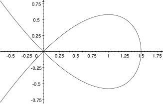
Figure 7: The homoclinic orbit for $\varepsilon=0$.

6.1 Approximating the unstable manifold

We first consider $\varepsilon=0.$ After a linear change of coordinates

$$\left(x,y\right)=C\left(u,v\right),$$

$$C=\left(\begin{array}[]{ll}1&-1\\ 1&1\end{array}\right),\qquad\qquad C^{-1}=\left(\begin{array}[]{cc}\frac{1}{2}&\frac{1}{2}\\ -\frac{1}{2}&\frac{1}{2}\end{array}\right),$$ (95)

the ODE becomes

$$\left(u,v\right)^{\prime}=F\left(u,v\right)=\left(\begin{array}[]{c}u-\frac{1}{2}\left(u-v\right)^{2}\\ -v-\frac{1}{2}\left(u-v\right)^{2}\end{array}\right).$$

Below we quickly describe how the unstable manifold can be approximated using the parametrization method (for a detailed overview of the method see [2]). We look for a function $K:\left(-r,r\right)\mathbb{\rightarrow R}^{2}$ and $R:\mathbb{R\rightarrow R}$ so that

$$F\circ K\left(\xi\right)=DK\left(\xi\right)R\left(\xi\right).$$ (96)

The Taylor coefficients can be computed by power matching in the equation (96). There is a certain freedom regarding the choice of the coefficients, and we have chosen them so that

$$K\left(\xi\right)=\left(\xi,K_{2}\left(\xi\right)\right).$$

For our coordinate change we expand (96) only to powers of three and choose

$$K_{2}\left(\xi\right) =-\frac{1}{6}\xi^{2}-\frac{1}{12}\xi^{3},$$

$$R\left(\xi\right) =\xi-\frac{1}{2}\xi^{2}-\frac{1}{6}\xi^{3}.$$

The set

$$W^{u}\approx\left\{\left(\xi,K_{2}\left(\xi\right)\right):\xi\in\left(-r,r\right)\right\},$$ (97)

is an approximation of the unstable manifold.

6.2 Approximating the stable manifold

In this section we also consider $\varepsilon=0$. The parametrization of the stable manifold follows from the reversing symmetry of the system: If we let $\Phi_{t}$ stand for the flow, and $S(x,y)=\left(x,-y\right)$, then

$$\Phi_{t}\left(S(q)\right)=S\left(\Phi_{-t}\left(q\right)\right).$$

This means that the stable manifold is parameterized by

$$w^{s}\left(\xi\right)=S\left(w^{u}\left(\xi\right)\right).$$

For our later consideration, it will be convenient to consider coordinates in which it the stable manifold is tangent to the $x$-axis. This can be obtained by taking (see (95) for the definition of $C$)

$$T=\left(\begin{array}[]{ll}0&1\\ -1&0\end{array}\right),\qquad\qquad\bar{C}=CT=\left(\begin{array}[]{cc}1&1\\ -1&1\end{array}\right)$$

and computing

$$w^{s}\left(\xi\right) =SC\left(\xi,K_{2}\left(\xi\right)\right)$$ (98)

$$=\bar{C}\left(\xi,-K_{2}\left(\xi\right)\right).$$

We can therefore take $\bar{C}$ as the linear change of coordinates, and in these local coordinates the stable manifold is parameterized by

$$\xi\rightarrow\left(\xi,-K_{2}\left(\xi\right)\right).$$ (99)

6.3 Suitable change of coordinates for the unstable manifold

Now we consider $\varepsilon\geq 0.$ We treat the system (94) in the coordinates $\left(x,\varepsilon,t,y\right)$,

$$\left(x,\varepsilon,t,y\right)^{\prime}=f\left(x,\varepsilon,t,y\right),$$ (100)

with the vector field

$$f\left(x,\varepsilon,t,y\right)=\left(y-\varepsilon\cos(t)y^{2},0,1,x-x^{2}\right).$$

Observe that for each $\varepsilon\geq 0$ we have the periodic orbit

$$\Lambda_{\varepsilon}=\left\{\left(0,\varepsilon,t,0\right):t\in\mathbb{S}^{1}\right\}.$$

We go through the following change of coordinates

$$\left(x,\varepsilon,t,y\right)=\tilde{C}_{u}\,\psi_{u}\left(\bar{x},\varepsilon,t,\bar{y}\right),$$ (101)

where $\tilde{C}$ is a linear change, motivated by (95),

$$\tilde{C}_{u}=\left(\begin{array}[]{llll}1&0&0&-1\\ 0&1&0&0\\ 0&0&1&0\\ 1&0&0&1\end{array}\right),\qquad\qquad\tilde{C}_{u}^{-1}=\left(\begin{array}[]{llll}\frac{1}{2}&0&0&\frac{1}{2}\\ 0&1&0&0\\ 0&0&1&0\\ -\frac{1}{2}&0&0&\frac{1}{2}\end{array}\right),$$

and $\psi_{u}$ is a nonlinear change motivated by (97),

$$\psi_{u}\left(\bar{x},\varepsilon,t,y\right)=\left(\bar{x},\varepsilon,t,\bar{y}+K_{2}\left(\bar{x}\right)\right).$$

The $\psi_{u}$ is simple to invert

$$\psi_{u}^{-1}\left(a,\varepsilon,t,b\right)=\left(a,\varepsilon,t,b-K_{2}\left(a\right)\right).$$

Remark 37

Our change of coordinates is independent of $\varepsilon$. It is motivated by the approximation of the manifold for $\varepsilon=0$, which is also a good approximation for small $\varepsilon$. For our method to work, the coordinates do not need to be perfectly aligned with the dynamics. An approximate alignment is sufficient.

It is a simple task (though slightly laborious) to derive the formula for the vector field in the local coordinates $\left(\bar{x},\varepsilon,t,\bar{y}\right)$

$$\tilde{f}\left(\bar{x},\varepsilon,t,\bar{y}\right)=\left(\tilde{f}_{1}\left(\bar{x},\varepsilon,t,\bar{y}\right),0,1,-K_{2}^{\prime}\left(\bar{x}\right)\tilde{f}_{1}\left(\bar{x},\varepsilon,t,\bar{y}\right)+\tilde{h}\left(\bar{x},\varepsilon,t,\bar{y}\right)\right),$$ (102)

where

$$\tilde{f}_{1}\left(\bar{x},\varepsilon,t,\bar{y}\right) =\bar{x}-\frac{1}{2}\varepsilon\left(\cos t\right)\left(\bar{x}+\bar{y}+K_{2}\left(\bar{x}\right)\right)^{2}-\frac{1}{2}\left(\bar{x}-\bar{y}-K_{2}\left(\bar{x}\right)\right)^{2},$$

$$\tilde{h}\left(\bar{x},\varepsilon,t,\bar{y}\right) =-\bar{y}-K_{2}\left(\bar{x}\right)+\frac{1}{2}\varepsilon\left(\cos t\right)\left(\bar{x}+\bar{y}+K_{2}\left(\bar{x}\right)\right)^{2}-\frac{1}{2}\left(\bar{x}-\bar{y}-K_{2}\left(\bar{x}\right)\right)^{2}.$$

6.4 Suitable change of coordinates for the stable manifold

The stable manifold of (100) coincides with the unstable manifold of an ODE with reversed sign:

$$\left(x,\varepsilon,t,y\right)^{\prime}=-f\left(x,\varepsilon,t,y\right).$$ (103)

Remark 38

We consider the formulation with reversed sign vector field, since in all our discussions we have talked about unstable manifolds. This way we can use our methods directly. The bounds on the unstable manifold of (103) will be the bounds for the stable manifold for (100).

We consider the change of coordinates

$$\left(x,\varepsilon,t,y\right)=\tilde{C}_{s}\,\psi_{s}\left(\bar{x},\varepsilon,t,\bar{y}\right),$$

with $\tilde{C}_{s}$ motivated by (98),

$$\tilde{C}_{s}=\left(\begin{array}[]{llll}1&0&0&1\\ 0&1&0&0\\ 0&0&1&0\\ -1&0&0&1\end{array}\right)\qquad\tilde{C}_{s}=\left(\begin{array}[]{cccc}\frac{1}{2}&0&0&-\frac{1}{2}\\ 0&1&0&0\\ 0&0&1&0\\ \frac{1}{2}&0&0&\frac{1}{2}\end{array}\right),$$

and $\psi_{s}$ motivated by (99),

$$\psi_{s}\left(\bar{x},\varepsilon,t,y\right) =\left(\bar{x},\varepsilon,t,\bar{y}-K_{2}\left(\bar{x}\right)\right),$$

$$\psi_{s}^{-1}\left(\bar{x},\varepsilon,t,y\right) =\left(\bar{x},\varepsilon,t,\bar{y}+K_{2}\left(\bar{x}\right)\right).$$

The vector field (103) rewritten in these local coordinates is

$$\hat{f}\left(\bar{x},\varepsilon,t,\bar{y}\right)=\left(\hat{f}_{1}\left(\bar{x},\varepsilon,t,\bar{y}\right),0,-1,K_{2}^{\prime}(\bar{x})\hat{f}_{1}\left(\bar{x},\varepsilon,t,\bar{y}\right)+\hat{h}\left(\bar{x},\varepsilon,t,\bar{y}\right)\right),$$ (104)

with

$$\hat{f}_{1}\left(\bar{x},\varepsilon,t,\bar{y}\right) =\bar{x}+\frac{1}{2}\varepsilon\left(\cos t\right)\left(-\bar{x}+\bar{y}-K_{2}\left(\bar{x}\right)\right)^{2}-\frac{1}{2}\left(\bar{x}+\bar{y}-K_{2}\left(\bar{x}\right)\right)^{2},$$

$$\hat{h}\left(\bar{x},\varepsilon,t,\bar{y}\right) =-\bar{y}+K_{2}\left(\bar{x}\right)+\frac{1}{2}\varepsilon\left(\cos t\right)\left(-\bar{x}+\bar{y}-K_{2}\left(\bar{x}\right)\right)^{2}+\frac{1}{2}\left(\bar{x}+\bar{y}-K_{2}\left(\bar{x}\right)\right)^{2}.$$

6.5 Bounds on the unstable and stable manifolds

In our computer assisted proof, we have used the vector field $\tilde{f}$ (see (102)), to establish the existence and bound for $W^{u}\left(\Lambda_{\varepsilon}\right)$ inside of the set

$$D=\left[-r,r\right]\times E\times\mathbb{S}^{1}\times\left[-rL(E),rL(E)\right],$$

for

$$r=2\cdot 10^{-4},$$

and for various parameter intervals $E$. The size on the set depends through $L(E)$ on the range $E$ of the parameter $\varepsilon$ considered. For $E=\left[0,10^{-3}\right]$, which is the first parameter interval we consider, we obtain that Theorem 30 can be applied with constants $\overrightarrow{\mu_{s,1}}$, $\overrightarrow{\mu_{s,2}}$, $\overrightarrow{\xi_{u,1}}$, $\overrightarrow{\xi_{u,1,P}}$, $\overrightarrow{\mu_{cs,1}}$, $\overrightarrow{\mu_{cs,2}}$, $\overrightarrow{\xi_{cu,1}}$ and $\overrightarrow{\xi_{cu,1,P}}$ with the following choice of the constant $L$:

$$L=L(E)=L\left(\left[0,10^{-3}\right]\right)=6.278276608\cdot 10^{-6}.$$

In our code, the $L(E)$ is chosen automatically by the program to be as small as possible to establish sharp bounds on the derivatives of $w^{cu}.$

From Theorem 30 we know that the function $w^{cu}$ is Lipschitz with constant $L(E)$. Thus,

$$\frac{\partial w^{cu}}{\partial\bar{x}}\left(D\right),\frac{\partial w^{cu}}{\partial\varepsilon}\left(D\right),\frac{\partial w^{cu}}{\partial t}\left(D\right)\in L\left(E\right)\cdot[-1,1].$$

Bounds on the second derivatives also depend on the choice of $E.$ They can be established using Theorem 36. For example, for $E=\left[0,10^{-3}\right]$, we obtained

$$M=M(E)=1.\,\allowbreak 127\,1\times 10^{-3}.$$

Thus, for $\varepsilon\in\left[0,10^{-3}\right],$

$$\frac{\partial^{2}w^{cu}}{\partial v\partial w}\left(D\right)\in 2M\cdot[-1,1]\qquad\text{for }v,w\in\{\bar{x},\varepsilon,t\}.$$

The bounds can then be transported through the change of coordinates (101). This is done automatically by the CAPD library, which has an implementation of rigorous manipulation on jets.

Similar bounds can be obtained for the stable manifold by considering the vector field $\hat{f}$ (with reversed time) given in (104). The bounds on the slope of the stable manifold and on the second derivatives are indistinguishable from those of the unstable manifold, up to the accuracy which we have used above to display results.

6.6 The transversal intersections of manifolds

We recall that by (20)

$$\delta\left(\varepsilon,\tau\right):=\pi_{x}p^{u}\left(\varepsilon,\tau\right)-\pi_{x}p^{s}\left(\varepsilon,\tau\right),$$

where $p^{u}$ and $p^{s}$ are defined in (21).

We first consider $\varepsilon\in\left[0,10^{-3}\right]$. In the left hand side of Figure 8 we give a plot of a computer assisted bound for

$$\tau\rightarrow\pi_{x}\frac{\partial p^{u}}{\partial\varepsilon}\left(\varepsilon,\tau\right)\qquad\text{and}\qquad\tau\rightarrow\pi_{x}\frac{\partial p^{s}}{\partial\varepsilon}\left(\varepsilon,\tau\right).$$

For $\tau$ close to $4.6$, for all $\varepsilon\in\left[0,10^{-3}\right]$ we have

$$\pi_{x}\frac{\partial p^{u}}{\partial\varepsilon}\left(\varepsilon,\tau\right)>\pi_{x}\frac{\partial p^{s}}{\partial\varepsilon}\left(\varepsilon,\tau\right),$$

hence for these $\tau$

$$\frac{d}{d\varepsilon}\delta\left(\varepsilon,\tau\right)>0.$$

Analogously, for the $\tau$ close to $4.8$ we have $\frac{d}{d\varepsilon}\delta\left(\varepsilon,\tau\right)<0.$ The right hand side of Figure 8 contains the plots of

$$\tau\rightarrow\pi_{x}\frac{\partial^{2}p^{u}}{\partial\tau\partial\varepsilon}\left(\varepsilon,\tau\right)\qquad\text{and}\qquad\tau\rightarrow\pi_{x}\frac{\partial^{2}p^{s}}{\partial\tau\partial\varepsilon}\left(\varepsilon,\tau\right).$$

For all $\varepsilon\in\left[0,10^{-3}\right]$ and the considered range of $\tau$ we have

$$\pi_{x}\frac{\partial^{2}p^{u}}{\partial\tau\partial\varepsilon}\left(\varepsilon,\tau\right)<0\qquad\text{and\qquad}\pi_{x}\frac{\partial^{2}p^{s}}{\partial\tau\partial\varepsilon}\left(\varepsilon,\tau\right)>0,$$

hence

$$\frac{d^{2}}{d\tau d\varepsilon}\delta\left(\varepsilon,\tau\right)<0.$$

This way, by using Theorem 9, we obtain a proof of the transversal intersections of $W^{u}\left(\Lambda_{\varepsilon}\right)$ with $W^{s}\left(\Lambda_{\varepsilon}\right)$ for $\varepsilon\in(0,10^{-3}].$ The computations needed for this result took under 3 seconds on a single 3GHz Intel i7 core processor.

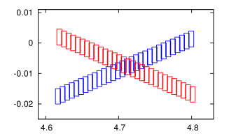
Figure 8: Left: The plot of the bounds on $\tau\rightarrow\pi_{x}\frac{\partial p^{u}}{\partial\varepsilon}\left(\varepsilon,\tau\right)$ in red and $\tau\rightarrow\pi_{x}\frac{\partial p^{s}}{\partial\varepsilon}\left(\varepsilon,\tau\right)$ in blue. Right: The plot of $\tau\rightarrow\pi_{x}\frac{\partial^{2}p^{u}}{\partial\tau\partial\varepsilon}\left(\varepsilon,\tau\right)$ in red and $\tau\rightarrow\pi_{x}\frac{\partial^{2}p^{s}}{\partial\tau\partial\varepsilon}\left(\varepsilon,\tau\right)$ in blue. In both plots we have $\tau$ on the $x$-axis. The bounds are for $\varepsilon\in\left[0,10^{-3}\right]$.

It turns out that the perturbation $\varepsilon=10^{-3}$ is relatively “large”. From such parameter we can directly observe, through rigorous numerics, that $W^{u}\left(\Lambda_{\varepsilon}\right)$ and $W^{s}\left(\Lambda_{\varepsilon}\right)$ intersect transversally. This can be seen by directly plotting bounds on $\tau\rightarrow\pi_{x}p^{u}\left(\varepsilon,\tau\right)$ and $\tau\rightarrow\pi_{x}p^{s}\left(\varepsilon,\tau\right)$. Such bounds, for $\varepsilon\in\left[10^{-3},10^{-3}+10^{-4}\right]$, are given in the left hand side plot of Figure 9. This way we establish that $W^{u}\left(\Lambda_{\varepsilon}\right)$ and $W^{s}\left(\Lambda_{\varepsilon}\right)$ intersect (see the left hand side plot in Figure 9). To show that this intersection is transversal we consider bounds on (right plot in Figure 9)

$$\tau\rightarrow\pi_{x}\frac{\partial p^{u}}{\partial\tau}\left(\varepsilon,\tau\right)\qquad\text{and}\qquad\tau\rightarrow\pi_{x}\frac{\partial p^{s}}{\partial\tau}\left(\varepsilon,\tau\right).$$

These bounds establish that for the investigated range of $\tau$, the function $\tau\rightarrow\delta\left(\varepsilon,\tau\right)$ is strictly decreasing. Thus, the intersection between $W^{u}\left(\Lambda_{\varepsilon}\right)$ and $W^{s}\left(\Lambda_{\varepsilon}\right)$ is transversal.

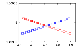
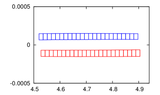
Figure 9: Left: The plot of $\tau\rightarrow\pi_{x}p^{u}\left(\varepsilon,\tau\right)$ in red and $\tau\rightarrow\pi_{x}p^{s}\left(\varepsilon,\tau\right)$ in blue. Right: The plot of $\tau\rightarrow\frac{\partial p^{u}}{\partial\tau}\left(\varepsilon,\tau\right)$ in red and $\tau\rightarrow\frac{\partial p^{s}}{\partial\tau}\left(\varepsilon,\tau\right)$ in blue. We have $\tau$ on the $x$-axis. The bounds are for $\varepsilon\in\left[10^{-3},10^{-3}+10^{-4}\right]$.

This procedure can be continued by considering other interval parameters. We have investigated the range $\left[10^{-3},10^{-2}\right]$, by dicing it into $90$ intervals of length $10^{-4}$. The results are given in Figure 10, where we have highlighted the bounds for $\varepsilon\in\left[10^{-3},10^{-3}+10^{-4}\right]$ in black. Thus, the black part of Figure 10 corresponds to Figure 9 (only in different scale on the vertical coordinate). In gray we have highlighted the bounds for $\varepsilon\in\left[10^{-2}-10^{-4},10^{-2}\right]$, which was the last of the $90$ considered parameter intervals. Each of the $90$ intervals took around half a second on a single 3GHz Intel i7 core processor. (The computation for the $90$ intervals in total took $54$ seconds on the single core.)

In sum, in this example we have established a computer assisted proof of transversal intersections of $W^{u}\left(\Lambda_{\varepsilon}\right)$ and $W^{s}\left(\Lambda_{\varepsilon}\right)$ for all $\varepsilon\in(0,10^{-2}]$. The whole computation time required under one minute on a single processor. There is no obstacle of course to continue such proof for larger $\varepsilon$. The subtle part was how to separate from $\varepsilon=0$. Once relatively far away, one can continue with ease.

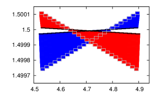
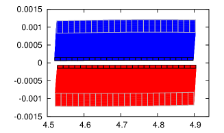
Figure 10: Left: The plot of $\tau\rightarrow\pi_{x}p^{u}\left(\varepsilon,\tau\right)$ in red and $\tau\rightarrow\pi_{x}p^{s}\left(\varepsilon,\tau\right)$ in blue. Right: The plot of $\tau\rightarrow\pi_{x}\frac{\partial p^{u}}{\partial\tau}\left(\varepsilon,\tau\right)$ in red and $\tau\rightarrow\pi_{x}\frac{\partial p^{s}}{\partial\tau}\left(\varepsilon,\tau\right)$ in blue. We have $\tau$ on the $x$-axis. The bounds are for $\varepsilon\in\left[10^{-3},10^{-2}\right]$.

7 Acknowledgements

We would like to thank Daniel Wilczak for his advice and discussions concerning higher order derivatives and jet manipulation in the CAPD library.

8 Appendix

8.1 Proof of Lemma 3

Proof. It is known (see for example [18, Sec. 3]) that the limit in the definition of logarithmic norms exists and the convergence is locally uniform with respect to $A$. We will reduce our question to this.

We have for $h\in(0,1]$ on compact sets of $A$’s

$$\frac{m(I+hA)-1}{h} =\frac{\frac{1}{\|(I+hA)^{-1}\|}-1}{h}$$

$$=\frac{\frac{1}{\|I-hA+O(h^{2})\|}-1}{h}$$

$$\leq\frac{\frac{1}{\|I-hA\|-O(h^{2})}-1}{h}$$

$$=\frac{\|I-hA\|^{-1}+O(h^{2})-1}{h}$$

$$=-\frac{\|I-hA\|-1}{h}\frac{1}{\|I-hA\|}+O(h)$$

$$\rightarrow-l(-A),\quad h\rightarrow 0$$

It is known that $l(A)$ is a convex function. Since $l(-A)$ is convex, $m_{l}(A)$ is concave.   

8.2 Proof of Theorem 5

Proof. Observe that from Lemma 3 it follows that

$$m_{l}(Df,W)=-\sup_{x\in W}l(-Df(x)).$$

From Theorem 4 applied to $x^{\prime}=-f(x)$ with initial conditions $x(t)$ and $y(t)$ we obtain

$$\|x(0)-y(0)\|\leq\exp\left(t\sup_{z\in W}l(-Df(z))\right)\|x(t)-y(t)\|.$$

Hence

$$\|x(0)-y(0)\|\exp\left(-t\sup_{z\in W}l(-Df(z))\right)\leq\|x(t)-y(t)\|.$$

Since $m(A)=-l(-A)$, our claim follows from the above.   

8.3 Proof of Lemma 7

Proof. We have

$$((I+hA)x|(I+hA)x) = ((I+hA)^{\top}(I+hA)x|x)$$

$$= \left(\left(I+h(A+A^{\top})\right)x|x\right)+h^{2}(A^{\top}Ax|x)$$

$$= \left(\left(I+h(A+A^{\top})\right)x|x\right)+O(h^{2}\|x\|^{2}\|A^{\top}A\|).$$

Therefore, (below we use the fact that $\sqrt{1+x}=1+\frac{1}{2}x+O\left(x^{2}\right)$)

$$\|I+hA\| = \max_{\|x\|=1}\sqrt{((I+hA)x|(I+hA)x))}$$

$$= \max_{\|x\|=1}\sqrt{\left(\left(I+h(A+A^{\top})\right)x|x\right)+O(h^{2}\|A^{\top}A\|)}$$

$$= \max_{\|x\|=1}\sqrt{1+h((A+A^{\top})x|x)+O(h^{2}\|A^{\top}A\|)}$$

$$= 1+\frac{h}{2}\max_{\|x\|=1}((A+A^{\top})x|x)+O(h^{2}),$$

where $O(h^{2})$ is uniform with respect to $A\in W$. Hence by (11)

$$\|I+hA\| = 1+h\max\{\lambda\in\text{Spectrum}((A+A^{\top})/2)\}+O(h^{2})$$

$$= 1+hl(A)+O(h^{2}),$$

which concludes the proof.   

8.4 Proof of Lemma 8

Proof. The proof follows from Lemma 7. All below estimates are clearly uniform over a compact set $W$ and $h\in[0,h_{0}]$, for $h_{0}$ which is sufficiently small $h_{0}=h_{0}(W)$.

We have (applying Lemma 7 in the 5th and (8) in the last line)

$$m(I+hA) = \frac{1}{\|(I+hA)^{-1}\|}$$

$$= \frac{1}{\|I-hA+O(h^{2})\|}$$

$$= \frac{1}{\|I-hA\|+O(h^{2})}$$

$$= \frac{1}{\|I-hA\|}+O(h^{2})$$

$$= \frac{1}{1+hl(-A)+O(h^{2})}+O(h^{2})$$

$$= 1-hl(-A)+O(h^{2})$$

$$= 1+hm_{l}(A)+O(h^{2}),$$

as required.   

8.5 Solving an implicit function problem in interval arithmetic

Consider $f:\mathbb{R}^{k}\times\mathbb{R}^{l}\rightarrow\mathbb{R}^{l}$. We wish to solve for $y$ satisfying

$$f(x,y\left(x\right))=0.$$

Consider $x\in\mathbb{R}^{k},y_{0}\in\mathbb{R}^{l},$ and a cube $Y=\prod_{i=1}^{l}\left[a_{i},b_{i}\right]\subset\mathbb{R}^{l}$ and define

$$N\left(x,y_{0},Y\right):=y_{0}-\left[\frac{\partial f}{\partial y}\left(x,Y\right)\right]^{-1}f\left(x,y_{0}\right).$$

If $N\left(x,y_{0},Y\right)\subset Y$, then by the interval Newton method $y(x)\in Y.$ In practice, we can consider a cube $X\subset\mathbb{R}^{k},$ verify that $N\left(X,y_{0},Y\right)\subset Y,$ obtaining that $y(x)\in Y$ for all $x\in Y$. The method can be further refined by appropriate choices of coordinates to improve the estimates (see for instance [4, section 4.1]).

References

- [1] V.I. Arnold, Instability of dynamical systems with several degrees of freedom, Sov. Math. Doklady, 5, 342 355, 1964.
- [2] X. Cabré, E. Fontich, R. de la Llave, The parameterization method for invariant manifolds III: overview and applications, J. Diff. Eq., 218 (2005) 444–515
- [3] R. Calleja, J-L. Figueras, Collision of invariant bundles of quasi-periodic attractors in the dissipative standard map. Chaos 22 (2012), no. 3, 033114, 10 pp. 37–99
- [4] M.J. Capinski, J.D. Mireles James, Validated computation of heteroclinic sets, http://arxiv.org/abs/1602.02973
- [5] M.J. Capinski, P. Zgliczynski, Cone conditions and covering relations for topologically normally hyperbolic manifolds, Discrete Contin. Dyn. Syst. 30 (2011) 641–670.
- [6] M.J. Capinski, P. Zgliczynski, Geometric proof for normally hyperbolic invariant manifolds, J. Diff. Eq., 259(2015) 6215–6286
- [7] R. Castelli, J-P. Lessard, J.D. Mireles James, Parameterization of invariant manifolds for periodic orbits I: Efficient numerics via the Floquet normal form. SIAM J. Appl. Dyn. Syst. 14 (2015), no. 1, 132–167.
- [8] S.N. Chow, J.K. Hale, J. Mallet-Paret An example of bifurcation to homoclinic orbits. J. Diff. Eqns. 37 (1980), 351–373.
- [9] G. Dahlquist, Stability and Error Bounds in the Numerical Intgration of Ordinary Differential Equations, Almqvist & Wiksells, Uppsala, 1958; Transactions of the Royal Institute of Technology, Stockholm, 1959.
- [10] A. Delshams, R. Ramirez-Ros, Melnikov Potential for Exact Symplectic Maps, Commun. Math. Phys. 190, 213 245 (1997)
- [11] A. Delshams, R. de la Llave, T. M. Seara. Geometric properties of the scattering map of a normally hyperbolic invariant manifold. Adv. Math., 217(3):1096–1153, 2008.
- [12] N. Fenichel, Asymptotic stability with rate conditions for dynamical systems, Bull. Amer. Math. Soc. 80 (1974) 346.
- [13] N. Fenichel, Asymptotic stability with rate conditions. II, Indiana Univ. Math. J. 26 (1) (1977) 81–93.
- [14] J-L. Figueras, A. Haro, Reliable computation of robust response tori on the verge of breakdown. SIAM J. Appl. Dyn. Syst. 11 (2012), no. 2, 597–628.
- [15] J. Guckenheimer and P. Holmes. Nonlinear Oscillations, Dynamical Systems and Bifurcations of Vector Fields. Springer, New York, 1983.
- [16] E. Hairer, S.P. Nørsett and G. Wanner, Solving Ordinary Differential Equations I, Nonstiff Problems, Springer-Verlag, Berlin Heidelberg 1987.
- [17] P. J. Holmes, J. E. Marsden. Melnikov’s method and Arnold diffusion for perturbations of integrable Hamiltonian systems. J. Math. Phys. 23 (1982), no. 4, 669–675.
- [18] T. Kapela and P. Zgliczyński, A Lohner-type algorithm for control systems and ordinary differential inclusions, Discrete Cont. Dyn. Sys. B, vol. 11(2009), 365-385.
- [19] J-P. Lessard, J.D. Mireles James, C. Reinhardt, Computer assisted proof of transverse saddle-to-saddle connecting orbits for first order vector fields. J. Dynam. Differential Equations 26 (2014), no. 2, 267–313.
- [20] S. M. Lozinskii, Error esitimates for the numerical integration of ordinary differential equations, part I, Izv. Vyss. Uceb. Zaved. Matematica,6 (1958), 52–90 (Russian)
- [21] Melnikov V.K On the stability of the center for time periodic perturbations. Trans. Moscow Math. Soc. 12 (1963), 1–57.
- [22] J. D. Mireles James, K. Mischaikow, Rigorous a posteriori computation of (un)stable manifolds and connecting orbits for analytic maps. SIAM J. Appl. Dyn. Syst. 12 (2013), no. 2, 957–1006.
- [23] K. Mischaikow, M. Mrozek, Conley index. Handbook of dynamical systems, Vol. 2, 393–460, North-Holland, Amsterdam, 2002.
- [24] H.J. Poincar . Sur le probleme des trois corps et les quations de la dynamique. Acta Mathematica, 13, 1 270, 1890.
- [25] S. Wiggins. Normally hyperbolic invariant manifolds in dynamical systems, volume 105 of Applied Mathematical Sciences. Springer-Verlag, New York, 1994.
- [26] D. Wilczak and P. Zgliczyński, Cr-Lohner algorithm, Schedae Informaticae, 20 (2011), pp. 9–46.
- [27] P. Zgliczyński, C1 Lohner algorithm. Found. Comput. Math. 2 (2002), no. 4, 429–465.