Next-to-leading order effective field theory $\Lambda N\to NN$ potential in coordinate space

Abstract

The potential in coordinate space for the $\Lambda N\to NN$ weak transition, which drives the weak decay of most hypernuclei, is derived within the effective field theory formalism up to next-to-leading order. This coordinate space potential allows us to discuss how the different contributions to the potential add up at the different scales. Explicit expressions are given for each two-pion-exchange diagram contributing to the interaction. The potential is also reorganized into spin and isospin operators, and the coefficient for each operator is given in analytical form and represented in coordinate space. The relevance of explicitly including the mass differences among the baryons appearing in the two-pion-exchange diagrams is also discussed in detail.

1 Introduction

The $\Lambda N\to NN$ interaction is the main mechanism driving the weak decay of heavy enough hypernuclei, see Refs. [1, 2] for recent reviews. In this transition, each of the two final nucleons obtains a kinetic energy of about $\frac{1}{2}(M_{\Lambda}-M_{N})=88$ MeV, which allows them to escape or break any hypernucleus. This is in contrast with the mesonic decay, $\Lambda\to N\pi$, which is responsible for the weak decay of the lightest hypernuclei and of the $\Lambda$ in free space. In this latter case the final nucleon and pion share a kinetic energy of only $\sim M_{\Lambda}-M_{N}-m_{\pi}=39$ MeV. For hypernuclei larger than $A=5$ this energy may not be enough for the nucleon to overcome the Pauli-blocking of the nuclear medium, and the one-nucleon induced decay mode dominates the decay process. The two-nucleon induced mechanism, $\Lambda NN\to NNN$, also contributes to the weak decay, but it only represents about 20$\%$ of the non-mesonic weak decay amplitude [3].

In hypernuclear experiments it is possible to measure the lifetime of a hypernucleus before it decays, as well as the angular and energetic distributions of the protons and neutrons emerging from the decay. From these quantities one can obtain information about three independent observables that constrain the two-body $\Lambda N\to NN$ interaction: the total non-mesonic decay rate, $\Gamma_{\Lambda N\to NN}$, the neutron- or proton-induced decay rates, $\Gamma_{\Lambda n\to nn}$ or $\Gamma_{\Lambda p\to np}$, and the asymmetry between the intensities of protons going up and down the polarization axis of the hypernucleus. This last measurement is related to the interference between the parity-conserving (PC) and parity-violating (PV) parts of the $\Lambda N\to NN$ amplitude. Using experimental data on the weak decay for both $s-$ and $p-$shell hypernuclei one is able to extract at most six independent observables.

The weak $|\Delta S|=1$ $\Lambda N$ interaction may also be constrained, in principle, by its experimental study in free space. On the one hand through direct $\Lambda p$ scattering, and on the other through the $\Lambda$ production reaction $np\to\Lambda p$. However both possibilities present great experimental difficulties, the former one due to the small lifetime of the $\Lambda$ ($\tau_{\Lambda}=2.63\cdot 10^{-10}$ s) and the corresponding difficulty to produce stable $\Lambda$ beams, and the latter due to the very small cross section for the $np\to\Lambda p$ transition ($10^{-12}$ mb) [4, 5, 6]. Currently we must rely on hypernuclear decay data to relate the theoretical description of this two-body interaction with the experiment. The experimental status and perspectives on non-mesonic weak decay has been recently reviewed in Ref. [7].

Theoretical studies of the non-mesonic weak decay amplitude were first based on one-meson-exchange (OME) models (see for example Refs. [8, 9, 10, 11]). These models describe the long range part of the interaction through the exchange of one pion, and the shorter ranges through the exchange of heavier mesons, the $\eta$, $\rho$, $\omega$, $K$ and $K^{*}$, which allow to mediate the strangeness exchange transition through weak vertices like $NNK$ or $\Lambda N\eta$. With the advent of the more systematic effective field theory (EFT) formalism, and in particular with its successful description of the NN strong interaction [12, 13], first steps were done in applying EFT also to the description of the non-mesonic weak decay. The EFT for the $\Lambda N\to NN$ potential was first studied at leading order (LO) in Refs. [14, 15, 16]. In Ref. [17] the EFT was further developed up to next-to-leading order (NLO), including all the possible two-pion-exchange (TPE) diagrams contributing to the transition. The potential was calculated in momentum space, and expressions in terms of master integrals were given separately for each diagram.

In the present work we provide all the needed expressions in coordinate space. The different contributions to the transition potential are written in terms of 20 operational structures. Notably, a simplified version of the transition potential, obtained neglecting the baryonic mass differences of virtual baryons, provides a compelling description of the full potential. These should be readily useful for ab-initio few-body computations of the weak decay of hypernuclei  [18, 19, 20, 21].

The manuscript is organized in the following way. In the beginning of Sect. 2 we review the EFT formalism used to calculate the non-mesonic weak transition. The EFT potentials up to NLO are derived in coordinate space and presented in terms of spin and isospin operators instead of diagrams. This allows us to plot for each operator the LO and the NLO potentials, and thus evaluate the magnitude of the two-pion exchanges in the $\Lambda N\to NN$ amplitude. The comparison is provided for each operational structure appearing in the transition potential. For the NLO, we derive approximate potentials neglecting the mass difference among the virtual baryons and compare them with the exact ones. In Sect. 3 we discuss the properties of the obtained potentials, including the comparison between the approximate and exact NLO potentials. A brief summary and conclusions are provided in Sect. 4. Details of the calculation and the expressions for the potentials in coordinate space are provided in the Appendices.

2 $\Lambda N\to NN$ EFT up to NLO

The EFT potential for the $\Lambda N\to NN$ transition is built as an expansion on a parameter $\frac{q}{M}$, $q$ and $M$ representing the low and high energy scales that characterize the interaction. These energy scales are determined by the typical momenta and masses involved in the weak decay process. Since the reaction is exothermic ($M_{\Lambda}>M_{N}$), the momenta of the emerging nucleons are larger than the ones for the initial $\Lambda$ and nucleon. The momenta of the $\Lambda$ and the nucleon in the center of mass are labelled as $\vec{p}$ and $-\vec{p}$, and the momenta of the final two nucleons as $\vec{p}\;^{\prime}$ and $-\vec{p}\;^{\prime}$. The low-energy scale in the expansion parameter depends thus on two momenta, the initial momentum $\vec{p}$, of roughly $200$ MeV, and the transferred momentum $\vec{q}\equiv\vec{p}\;^{\prime}-\vec{p}$, of the order of $400$ MeV.

Besides the $\Lambda$ and the nucleon we include the pion and the kaon as virtual mesons to be exchanged among the baryons and the $\Sigma$ as an intermediate baryonic state. Therefore, the characteristic low-energy scales are also the pion and kaon masses and the mass differences between the $\Lambda$, the $\Sigma$ and the nucleon. For the high-energy scale we take the chiral symmetry breaking scale, which is of the order of the mass of the baryons appearing in the interaction, around $1000$ MeV.

Once the expansion parameter and the degrees of freedom are defined we use Weinberg power-counting [22] to organize the potential into the different orders. At LO the potential includes the exchanges of the lightest pseudoscalar mesons and the non-derivative operators representing contact interactions. The $\eta$-exchange is not included due to its small coupling, thus the one-meson-exchanges consist of the one-pion- and one-kaon-exchanges (OPE and OKE). The NLO includes all the possible ways in which the $\Lambda$ and the nucleon can exchange two pions and the contact interactions containing one or two powers of momenta. The kaon-pion and the two-kaon exchange are not included in the NLO, first because their contribution is expected to be much smaller due to the larger mass of the kaon, and also to avoid adding further unknown (and therefore, model dependent) couplings to the theory.

The Feynman diagrams corresponding to the LO and NLO are shown respectively in Figs. 1 and 2.

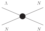
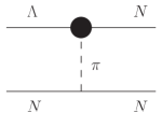
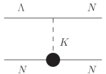
Figure 1: Leading-order Feynman diagrams contributing to the $\Lambda N\to NN$ process. They correspond, in order, to the contact interactions, the one-pion exchange and the one-kaon exchange. The solid dot represents the weak vertex.

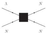
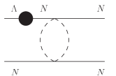
		(a)
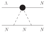
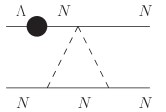
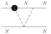
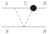
(b)	(c)	(d)	(e)
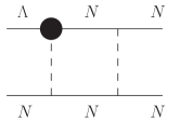
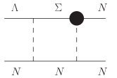
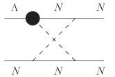
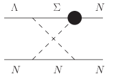
(f)	(g)	(h)	(i)

Figure 2: Contact interactions and two-pion exchanges contributing at next-to-leading order. The solid square represents operators at order ${\cal O}(q)$ and ${\cal O}(q^{2})$ and the solid vertex represents the weak vertex.

The expressions for the potentials in momentum space for the $\Lambda N\to NN$ transition as well as details of their derivations can be found in Ref. [17]. They are given for each possible diagram contributing to the transition and explicitly considering the mass differences between the $\Lambda$, the $\Sigma$ and the nucleon. In this section we take these potentials and the mathematical formalism used in their derivation to calculate them in coordinate space.

2.1 Leading order contributions

At leading order there are only two operational structures contributing to the contact part of the interaction, $\hat{1}$ and $\vec{\sigma}_{1}\cdot\vec{\sigma}_{2}$, and they are the same in momentum and coordinate space. $\vec{\sigma}_{1}$ and $\vec{\sigma}_{2}$ are the Pauli matrices connecting the spins of the upper and bottom baryons of the contact diagram in Fig. 1. The one-pion and one-kaon exchanges in momentum space consist of a non-relativistic propagator, $\frac{1}{m_{\alpha}^{2}+\vec{q}\,^{2}}$, which depends on the mass and momentum of the meson, $m_{\alpha}$ and $\vec{q}$, and the parity-violating and tensor structures $\vec{\sigma}_{2}\cdot\vec{q}$ and $(\vec{\sigma}_{1}\cdot\vec{q}\,)(\vec{\sigma}_{1}\cdot\vec{q}\,)$ [16]. They are straightforward to calculate in coordinate space by making the replacement $\vec{q}\to-i\vec{\nabla}$ in the Fourier transform. For example, for a PV term $\vec{\sigma}\cdot\vec{q}\,$ accompanying a general function $f(q)$,

$$\int\frac{d^{3}q}{(2\pi)^{3}}e^{i\vec{q}\cdot\vec{r}}f(q)\vec{\sigma}\cdot\vec{q}=-i\vec{\sigma}\cdot\vec{\nabla}\int\frac{d^{3}q}{(2\pi)^{3}}e^{i\vec{q}\cdot\vec{r}}f(q).$$ (1)

The remaining integrand $f(q)$ only contains the propagator (multiplied by couplings and masses), and thus one only needs to apply $\vec{\sigma}_{2}\cdot\vec{\nabla}$ and $(\vec{\sigma}_{1}\cdot\vec{\nabla})(\vec{\sigma}_{2}\cdot\vec{\nabla})$ to its Fourier transform, $\frac{e^{-m_{\alpha}r}}{4\pi r}$. We express both the OPE and the OKE potentials as

$$V_{\alpha}(r)= G_{F}m_{\pi}^{2}\frac{e^{-m_{\alpha}r}}{12\pi r^{3}}\left[\hat{A}_{\alpha}3r(1+m_{\alpha}r)\,i\vec{\sigma}_{\alpha}\cdot\hat{r}+\hat{B}_{\alpha}m_{\alpha}^{2}r^{2}\,\vec{\sigma}_{1}\cdot\vec{\sigma}_{2}+\hat{B}_{\alpha}\left(3+3m_{\alpha}r+m_{\alpha}^{2}r^{2}\right)\hat{S}_{12}(\hat{r})\right],$$ (2)

where the subindex $\alpha$ distinguishes between the pion ($\alpha=\pi$) and the kaon ($\alpha=K$) exchanges and their corresponding operators, masses, and couplings. $\hat{S}_{12}(\hat{r})\equiv 3\vec{\sigma}_{1}\cdot\hat{r}\vec{\sigma}_{2}\cdot\hat{r}-\vec{\sigma}_{1}\cdot\vec{\sigma}_{2}$ is the tensor operator, and $\vec{\sigma}_{\pi}=\vec{\sigma}_{2}$, $\vec{\sigma}_{K}=\vec{\sigma}_{1}$. $G_{F}m_{\pi}^{2}=2.21\cdot 10^{-7}$ is the Fermi constant, and $m_{\pi}=138$ MeV and $m_{K}=495$ MeV are the masses of the pion and the kaon. The isospin operators and the strong and weak couplings are encapsulated in $\hat{A}_{\alpha}$ and $\hat{B}_{\alpha}$, which are defined as [11] $\hat{A}_{\pi}=-\frac{g_{NN\pi}A_{\pi}}{2M_{N}}\,\vec{\tau}_{1}\cdot\vec{\tau}_{2}$, $\hat{B}_{\pi}=-\frac{g_{NN\pi}B_{\pi}}{4M_{N}\overline{M}}\,\vec{\tau}_{1}\cdot\vec{\tau}_{2}$, $\hat{A}_{K}=\frac{g_{\Lambda NK}A_{\pi}}{2\overline{M}}\,(\frac{1}{2}C_{K}^{PV}+D_{K}^{PV}+\frac{1}{2}C_{K}^{PV}\vec{\tau}_{1}\cdot\vec{\tau}_{2})$, and $\hat{B}_{K}=-\frac{g_{\Lambda NK}A_{\pi}}{4M_{N}\overline{M}}\,(\frac{1}{2}C_{K}^{PC}+D_{K}^{PC}+\frac{1}{2}C_{K}^{PC}\vec{\tau}_{1}\cdot\vec{\tau}_{2})$. $M_{N}=939$ MeV is the mass of the nucleon, $\overline{M}=\frac{1}{2}(M_{\Lambda}+M_{N})=1027$ MeV is the average mass of the nucleon and the $\Lambda$, and $\vec{\tau}$ are the isospin Pauli matrices. We take the values for the strong couplings $g_{NN\pi}=13.16$ and $g_{\Lambda NK}=-13.61$ from the Nijmegen 97f model [23]. The weak pionic couplings $A_{\pi}=1.05$ and $B_{\pi}=-7.15$ are fixed by the mesonic decay of the $\Lambda$, while the kaonic ones $C_{K}^{PC}=-18.9$, $D_{K}^{PC}=6.63$, $C_{K}^{PC}=0.76$ and $D_{K}^{PC}=2.09$ are derived using SU(3) symmetry.

We have followed this procedure also in the NLO so both orders are calculated in the same way. However one may also regularize the OME potentials through form factors and directly Fourier-transform the whole expressions. The results only differ in the shortest range of the interaction. Also note that in these expressions we have neglected the temporal part of the relativistic transferred momentum in the mesonic propagators, i.e. $q_{0}=\frac{1}{2}(M_{\Lambda}-M_{N})$ in $\frac{1}{\vec{q}\,^{2}+m_{\alpha}^{2}-q_{0}^{2}}$. In order to take it into account one only needs to replace $m_{\alpha}\to\sqrt{m_{\alpha}^{2}-q_{0}^{2}}$ in the expressions above. In this case the potentials would have the same Yukawa form but would decay slower due to their smaller effective masses.

In Fig. 3 we plot the OPE and OKE potentials of Eq. (2). The coefficients for the isospin operators $\hat{1}$ and $\vec{\tau}_{1}\cdot\vec{\tau}_{2}$ are labelled respectively $V$ and $W$. For each of the three spin operational structures we plot the OPE, which only contains the isospin-isospin operator, together with the two isospin contributions from the OKE.

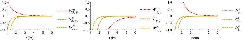
Figure 3: Weak $\Lambda N\to NN$ potentials stemming from the one-pion and one-kaon exchanges for the three spin operators to which they contribute. The potentials are labelled $V$ and $W$ corresponding to the two isospin scalar operators $\hat{1}$ and $\vec{\tau}_{1}\cdot\vec{\tau}_{2}$. The potentials units are MeV, the momentum $|\vec{p}\,|$ is fixed to $150$ MeV.

2.2 Next-to-leading order contributions

The contact part of the NLO potential contains all the possible operational structures that can be built with the momenta $\vec{p}$, $\vec{q}$ and the Pauli matrices $\vec{\sigma}_{1}$ and $\vec{\sigma}_{2}$. There are 18 in total —6 at ${\cal O}(q)$ and 12 at ${\cal O}(q^{2})$— and they are shown in Table 1. The corresponding operators in coordinate space are obtained by replacing $\vec{q}\to\vec{r}$ and $\vec{p}\to-i\vec{\nabla}$.

${\cal O}$($q$)	$\vec{\sigma}_{1}\cdot\vec{q}\,$, $\vec{\sigma}_{2}\cdot\vec{q}\,$, $\vec{\sigma}_{1}\cdot\vec{p}\,$, $\vec{\sigma}_{2}\cdot\vec{p}\,$, $(\vec{\sigma}_{1}\times\vec{\sigma}_{2})\cdot\vec{q}\,$, $(\vec{\sigma}_{1}\times\vec{\sigma}_{2})\cdot\vec{p}\,$,
${\cal O}$($q^{2}$)	$\vec{q}\,^{2}$, $\vec{p}\,^{2}$, $\vec{q}\,\cdot\vec{p}\,$, $(\vec{\sigma}_{1}\cdot\vec{\sigma}_{2})\vec{q}\,^{2}$, $(\vec{\sigma}_{1}\cdot\vec{\sigma}_{2})\vec{p}\,^{2}$, $(\vec{\sigma}_{1}\cdot\vec{\sigma}_{2})\vec{q}\,\cdot\vec{p}\,$
	$\vec{\sigma}_{1}\cdot(\vec{q}\,\times\vec{p}\,)$, $\vec{\sigma}_{2}\cdot(\vec{q}\,\times\vec{p}\,)$, $(\vec{\sigma}_{1}\cdot\vec{p}\,)(\vec{\sigma}_{2}\cdot\vec{p}\,)$,
	$(\vec{\sigma}_{1}\cdot\vec{q}\,)(\vec{\sigma}_{2}\cdot\vec{p}\,)$, $(\vec{\sigma}_{1}\cdot\vec{p}\,)(\vec{\sigma}_{2}\cdot\vec{q}\,)$, $(\vec{\sigma}_{1}\cdot\vec{q}\,)(\vec{\sigma}_{2}\cdot\vec{q}\,)$.

Table 1: Contact NLO operators containing one and two powers of momenta $\vec{q}$, $\vec{p}$. $\vec{\sigma}_{1}$ and $\vec{\sigma}_{2}$ are the Pauli matrices.

The two-pion-exchange contribution to the NLO potential is much more involved due to the various integrals appearing in the nine loop diagrams of Fig. 2. Terms corresponding to mass differences between the $\Lambda$, the $\Sigma$ and the nucleon also appear in the propagators of these NLO potentials, and neglecting these terms makes the expressions considerably simpler. However, it is not clear how these potentials change when these mass differences are neglected. In order to evaluate precisely this effect we derive in the next two subsections both the approximate and non-approximate potentials and reorganize them in terms of operators. Both cases contribute to 20 spin and isospin operational structures and are written in the following form:

$$V(r)= V_{1}+W_{1}(\vec{\tau}_{1}\cdot\vec{\tau}_{2})+V_{(\vec{\sigma}_{1}\cdot\vec{\sigma}_{2})}(\vec{\sigma}_{1}\cdot\vec{\sigma}_{2})+W_{(\vec{\sigma}_{1}\cdot\vec{\sigma}_{2})}(\vec{\sigma}_{1}\cdot\vec{\sigma}_{2})(\vec{\tau}_{1}\cdot\vec{\tau}_{2})$$ (3)

$$+V_{(\hat{r}\cdot\hat{p}\,)}(\hat{r}\cdot\hat{p}\,)+W_{(\hat{r}\cdot\hat{p}\,)}(\hat{r}\cdot\hat{p}\,)(\vec{\tau}_{1}\cdot\vec{\tau}_{2})+V_{(\vec{\sigma}_{1}\cdot\hat{r})}(\vec{\sigma}_{1}\cdot\hat{r})+W_{(\vec{\sigma}_{1}\cdot\hat{r})}(\vec{\sigma}_{1}\cdot\hat{r})(\vec{\tau}_{1}\cdot\vec{\tau}_{2})$$

$$+V_{(\vec{\sigma}_{1}\cdot\vec{\sigma}_{2})(\hat{r}\cdot\hat{p}\,)}(\vec{\sigma}_{1}\cdot\vec{\sigma}_{2})(\hat{r}\cdot\hat{p}\,)+W_{(\vec{\sigma}_{1}\cdot\vec{\sigma}_{2})(\hat{r}\cdot\hat{p}\,)}(\vec{\sigma}_{1}\cdot\vec{\sigma}_{2})(\hat{r}\cdot\hat{p}\,)(\vec{\tau}_{1}\cdot\vec{\tau}_{2})$$

$$+V_{(\vec{\sigma}_{1}\cdot\hat{r})(\vec{\sigma}_{1}\cdot\hat{p}\,)}(\vec{\sigma}_{1}\cdot\hat{r})(\vec{\sigma}_{1}\cdot\hat{p}\,)+W_{(\vec{\sigma}_{1}\cdot\hat{r})(\vec{\sigma}_{1}\cdot\hat{p}\,)}(\vec{\sigma}_{1}\cdot\hat{r})(\vec{\sigma}_{1}\cdot\hat{p}\,)(\vec{\tau}_{1}\cdot\vec{\tau}_{2})$$

$$+V_{\vec{\sigma}_{1}\cdot(\hat{r}\times\hat{p}\,)}\vec{\sigma}_{1}\cdot(\hat{r}\times\hat{p}\,)+W_{\vec{\sigma}_{1}\cdot(\hat{r}\times\hat{p}\,)}\vec{\sigma}_{1}\cdot(\hat{r}\times\hat{p}\,)(\vec{\tau}_{1}\cdot\vec{\tau}_{2})$$

$$+V_{\vec{\sigma}_{2}\cdot(\hat{r}\times\hat{p}\,)}\vec{\sigma}_{2}\cdot(\hat{r}\times\hat{p}\,)+W_{\vec{\sigma}_{2}\cdot(\hat{r}\times\hat{p}\,)}\vec{\sigma}_{2}\cdot(\hat{r}\times\hat{p}\,)(\vec{\tau}_{1}\cdot\vec{\tau}_{2})$$

$$+V_{(\vec{\sigma}_{1}\times\vec{\sigma}_{2})\cdot\hat{r}}(\vec{\sigma}_{1}\times\vec{\sigma}_{2})\cdot\hat{r}+W_{(\vec{\sigma}_{1}\times\vec{\sigma}_{2})\cdot\hat{r}}(\vec{\sigma}_{1}\times\vec{\sigma}_{2})\cdot\hat{r}(\vec{\tau}_{1}\cdot\vec{\tau}_{2})$$

$$+V_{\hat{S}_{12}}\hat{S}_{12}(\hat{r})+W_{\hat{S}_{12}}\hat{S}_{12}(\hat{r})(\vec{\tau}_{1}\cdot\vec{\tau}_{2}).$$

2.2.1 Potentials neglecting baryonic mass differences

Neglecting $M_{\Lambda}-M_{N}$ and $M_{\Sigma}-M_{\Lambda}$ in the NLO potentials in momentum space of Ref. [17] we obtain their expressions in terms of a set of integrals as shown in A.1. These integrals are characteristic to the topologies and vertices of the diagrams contributing to the $\Lambda N\to NN$ transition. They depend on the number of propagators, the number of integrated momenta in the numerator, and the tensor structure —formed by Kronecker deltas $\delta_{ij}$ and transferred momenta $\vec{q}_{i}$— to which they contribute. However, all of them can be related through Veltman-Passarino reductions [24] to the four following integrals,

$$B(q)\equiv\, \frac{1}{i}\int\frac{d^{4}l}{(2\pi)^{4}}\frac{1}{l^{2}-m^{2}+i\epsilon}\frac{1}{(l+q)^{2}-m^{2}+i\epsilon}=-\frac{1}{8\pi^{2}}L(q),$$ (4)

$$I(q)\equiv\, \frac{1}{i}\int\frac{d^{4}l}{(2\pi)^{4}}\frac{1}{l^{2}-m^{2}+i\epsilon}\frac{1}{(l+q)^{2}-m^{2}+i\epsilon}\frac{1}{-l_{0}+i\epsilon}=-\frac{1}{4\pi}A(q),$$

$$J(q)\equiv\, \frac{1}{i}\int\frac{d^{4}l}{(2\pi)^{4}}\frac{1}{l^{2}-m^{2}+i\epsilon}\frac{1}{(l+q)^{2}-m^{2}+i\epsilon}\frac{1}{-l_{0}+i\epsilon}\frac{1}{-l_{0}+i\epsilon}=\frac{1}{2\pi^{2}}\frac{1}{4m^{2}+q^{2}}L(q),$$

$$K(q)\equiv\, \frac{1}{i}\int\frac{d^{4}l}{(2\pi)^{4}}\frac{1}{l^{2}-m^{2}+i\epsilon}\frac{1}{(l+q)^{2}-m^{2}+i\epsilon}\frac{1}{-l_{0}-q_{0}^{\prime}+i\epsilon}\frac{1}{l_{0}+i\epsilon}=-J(q)+\frac{1}{2\pi q_{0}^{\prime}}A(q),$$

where

$$A(q)\equiv \frac{1}{2|\vec{q}\,|}\arctan\left(\frac{|\vec{q}\,|}{2m}\right),$$ (5)

$$L(q)\equiv \frac{\sqrt{4m^{2}+|\vec{q}\,|^{2}}}{|\vec{q}\,|}\ln\left(\frac{\sqrt{4m^{2}+|\vec{q}\,|^{2}}+|\vec{q}\,|}{2m}\right).$$

These are the simplest integrals that appear, in order, in the ball, triangle, crossed box, and box diagrams. A constant term in $B$ has been obviated since its Fourier transform is ill defined and is already considered by the contact interactions. In these equations and in the rest of the manuscript we denote the mass of the pion $m$ and the relativistic transferred momentum $q$. The temporal part of $q$, $q_{0}$, depends on the baryonic mass differences and has been neglected. $q_{0}^{\prime}$ is of the same order than $q_{0}$ and in principle it appears in the baryonic propagators of the four integrals. It has been neglected in all of them except in the last one, $K$, in order to avoid the pinch singularity characteristic of the box diagrams. In the final result of $K$ $q_{0}^{\prime}$ is also neglected except in the divergent term $\frac{1}{q_{0}^{\prime}}$.

The potentials thus depend only on $A(q)\vec{q}\,^{2n}$, $L(q)\vec{q}\,^{2n}$ and $\frac{L(q)}{4m^{2}+q^{2}}\vec{q}\,^{2n}$, where $n=0,1,2$, and the same terms but accompanied by spin structures (see A.2). To calculate the potentials in coordinate space we only need to Fourier transform this set of functions. All these Fourier transforms can be written in terms of exponentials and Bessel functions of order zero and one that depend on $2mr$ ($K_{0}(2mr)$ and $K_{1}(2mr)$). For example, for the simplest cases we have:

$$\mathcal{F}\left[A(q)\right] =\frac{e^{-2mr}}{8\pi r^{2}},$$ (6)

$$\mathcal{F}\left[L(q)\right] =-\frac{m}{2\pi r^{2}}K_{1}(2mr),$$

$$\mathcal{F}\left[\frac{L(q)}{4m^{2}+q^{2}}\right] =\frac{1}{4\pi r}K_{0}(2mr).$$

The explicit expressions for each operator coefficient of Eq. (3) in terms of the Bessel functions and exponentials are shown in A.2. We plot these coefficients in Fig. 4. For each spin operator we have the two isospin scalar contributions, $\hat{1}$ and $\vec{\tau}_{1}\cdot\vec{\tau}_{2}$, labelled as $V$ and $W$.

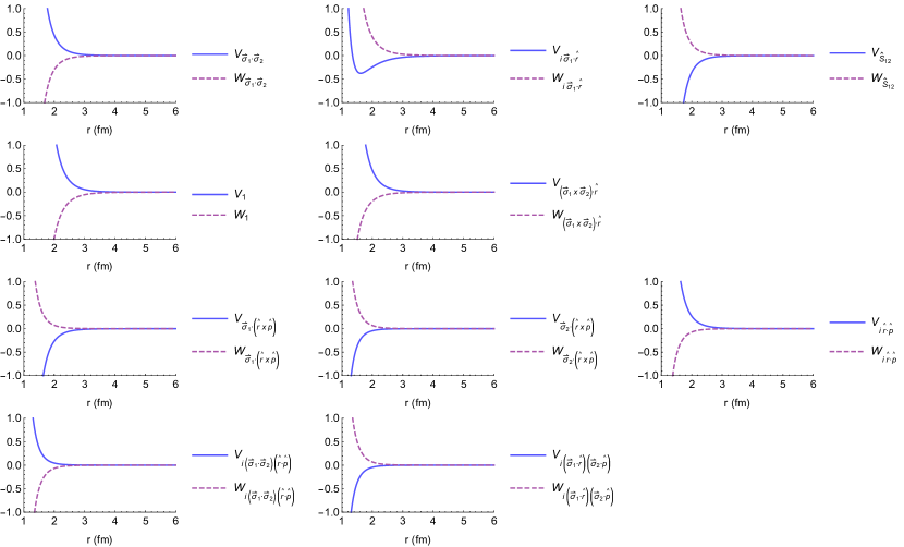
Figure 4: Weak $\Lambda N\to NN$ potentials arising from the two-pion exchanges. The units of the potentials are MeV. $|\vec{p}\,|$ is fixed to $150$ MeV.

2.2.2 Potentials considering baryonic mass differences

In the case in which the terms $q_{0}$ and $q_{0}^{\prime}$ are explicitly considered it is easier to calculate the necessary integrals directly in coordinate space. These are labelled again according to the diagram in which they appear, namely $B$, $I$, $J$ and $K$ for the ball, triangle, crossed-box, and box diagrams. The relativistic subindices $\mu...\nu$ correspond to the momenta appearing in the numerator:

$$B_{\mu...\nu}(q)= \frac{1}{i}\int\frac{d^{3}q}{(2\pi)^{3}}e^{i\vec{q}\cdot\vec{r}}\int\frac{d^{4}l}{(2\pi)^{4}}\frac{1}{l^{2}-m^{2}+i\epsilon}\frac{1}{(l+q)^{2}-m^{2}+i\epsilon}l_{\mu}...l_{\nu},$$ (7)

$$I_{\mu...\nu}(q)= \frac{1}{i}\int\frac{d^{3}q}{(2\pi)^{3}}e^{i\vec{q}\cdot\vec{r}}\int\frac{d^{4}l}{(2\pi)^{4}}\frac{1}{l^{2}-m^{2}+i\epsilon}\frac{1}{(l+q)^{2}-m^{2}+i\epsilon}\frac{1}{-l_{0}-q_{0}^{\prime}+i\epsilon}l_{\mu}...l_{\nu},$$

$$J_{\mu...\nu}(q)= \frac{1}{i}\int\frac{d^{3}q}{(2\pi)^{3}}e^{i\vec{q}\cdot\vec{r}}\int\frac{d^{4}l}{(2\pi)^{4}}\frac{1}{l^{2}-m^{2}+i\epsilon}\frac{1}{(l+q)^{2}-m^{2}+i\epsilon}\frac{1}{-l_{0}-q_{0}^{\prime}+i\epsilon}\frac{1}{-l_{0}+i\epsilon}l_{\mu}...l_{\nu},$$

$$K_{\mu...\nu}(q)= \frac{1}{i}\int\frac{d^{3}q}{(2\pi)^{3}}e^{i\vec{q}\cdot\vec{r}}\int\frac{d^{4}l}{(2\pi)^{4}}\frac{1}{l^{2}-m^{2}+i\epsilon}\frac{1}{(l+q)^{2}-m^{2}+i\epsilon}\frac{1}{-l_{0}-q_{0}^{\prime}+i\epsilon}\frac{1}{l_{0}+i\epsilon}l_{\mu}...l_{\nu}.$$

When the integrals also contain transferred momenta $\vec{q}_{i}$ in the numerators we can make the replacement $\vec{q}_{i}\to-i\vec{\nabla}_{i}$ and calculate them in terms of derivatives of the previous ones. These integrals will contain tensor structures formed by Kronecker deltas and vectors $\vec{r}_{i}$. The coefficients for each structure are defined in B.1, and the potentials for each diagram are shown in B.2. We reorganize again these potentials in terms of the spin operators of Eq. (3) and show the corresponding expressions also in B.2. In contrast with the case in which $M_{\Lambda}-M_{N}$ is neglected, now the potentials contain imaginary parts. This is because the initial masses are larger than the final ones and therefore the process is not unitary. In figs. 5 and 6 we plot the real and imaginary parts of the NLO potentials for each operator, respectively.

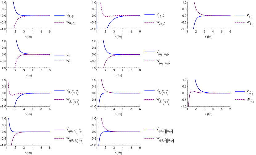
Figure 5: Real part of the two-pion-exchange potentials for the $\Lambda N\to NN$ transition. The units of the potentials are MeV, $|\vec{p}\,|$ is fixed to 150 MeV.

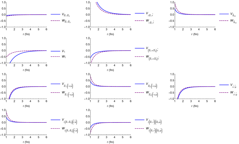
Figure 6: Imaginary part of the two-pion-exchange potentials for the $\Lambda N\to NN$ transition. The units of the potentials are MeV, $|\vec{p}\,|$ is fixed to 150 MeV.

3 Coordinate space potentials

In this section we first discuss how the LO and NLO potentials contribute to the different spin-isospin operational structures listed in Table 1. Secondly, we analyze the effect of neglecting the baryonic mass differences in the baryonic propagators.

3.1 Contributions from the OPE, OKE and TPE

The LO potential is represented in Fig. 3 and the NLO one in Figs. 4, 5, and 6. In the long range the $\Lambda N\to NN$ potential is clearly dominated by the one-pion-exchange. The one-kaon exchange is shorter ranged and interferes destructively with the OPE in the spin-spin and tensor potentials and constructively in the PV one.

At NLO the potential contains many more operational structures than the LO OPE and OKE, which allows for many more possible spin $\Lambda N\to NN$ transitions. For each spin operator the two isospin scalar contributions contribute with opposite signs as can be noticed in Fig. 4.

In Fig. 7 we plot together the LO and the NLO potentials for each of the three LO spin operators. The typical range of the two-pion exchanges is shorter than the one-meson exchanges. Above 2 fm the pion dominates the interaction, while in shorter ranges the NLO potential may surpass it, as seen for example in the spin-spin case. The one-kaon exchange decays faster than the one-pion exchange and is already dominated by the NLO in the medium range. For each operator the two-pion exchanges represent a noticeable part of the $\Lambda N\to NN$ amplitude. Moreover for certain transitions the 20 spin and isospin operators may interfere constructively, rendering a greater importance to the two-pion exchange than the one inferred from Fig. 7.

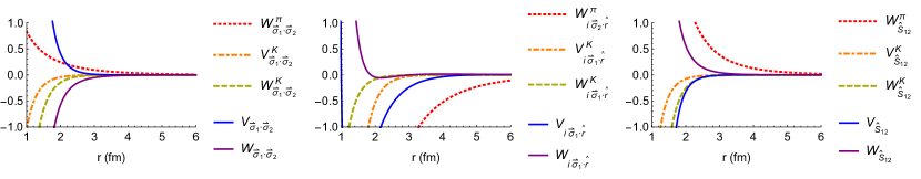
Figure 7: One-meson and two-pion exchange potentials for the three LO spin operators. For each of these operators the OPE and OKE are labelled with the superindices $\pi$ and $K$, and the scalar and isospin-isospin two-pion exchanges with $V$ and $W$. The units of the potentials are MeV, $|\vec{p}\,|$ is fixed to 150 MeV.

3.2 NLO potentials in the $M_{\Lambda}=M_{\Sigma}=M_{N}$ limit

In the SU(3) chiral effective Lagrangian the different octet masses appear at second order due to the explicit symmetry breaking term involving different quark masses. One can consider then an average mass for the baryon $\overline{M}$ plus a term of order ${\cal O}(q^{2})$. With this approximation the potentials for the $\Lambda N\to NN$ transition are purely real, since the initial and final masses are considered the same. Besides this feature, the explicit effect on the real part of the potentials is difficult to predict due to the complexity of the calculation.

In Fig. 8 we have plotted together the real parts of the NLO potentials obtained with and without the approximation. Only in one of the twenty operational structures we see a relevant qualitative change in the potentials. All of them maintain its attractive or repulsive character, however the PV isospin scalar $\vec{\sigma}_{1}\cdot\hat{r}$ structure becomes much more attractive when the different masses are considered. Except for that amplitude, the changes in all other structures are also fairly small from a quantitative point of view. We do not find any common pattern —some become slightly smaller and some slightly larger—. From a practical point of view, the NLO potentials obtained considering the terms $q_{0}$ and $q_{0}^{\prime}$ are certainly more precise, but also much more complicated and computationally time consuming to calculate. Thus, we expect that for any practical application to compute non-mesonic weak decay rates, the approximate potentials should be accurate enough.

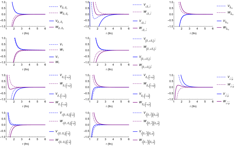
Figure 8: Comparison between the real part of the potentials with $q_{0}=q_{0}^{\prime}=0$ (dashed lines) and with $q_{0}\neq 0$, $q_{0}^{\prime}\neq 0$ (solid lines). The potential units are MeV, $|\vec{p}\,|$ is fixed to 150 MeV.

3.3 Contact part of the interaction

The EFT potential for the weak $|\Delta S|=1$ $\Lambda N$ interaction includes de medium and long range OPE, OKE and TPE diagrams as well as a series of contact interactions represented by the terms of Table 1. The coefficients of these terms, or the low energy constants (LECs), describe the short range physics and must be fixed by experiment. In Ref. [16] the LO LECs were constrained using recent experimental data on non-mesonic weak decay of s- and p-shell hypernuclei. It was found that different sets of values of the LO LECs could fit the data with a reasonable $\chi^{2}$. With the current status of experimental data for the non-mesonic weak decay of hypernuclei it is not possible to fix the 20 LECs characteristic of this interaction. Even with more accurate data there will always remain the difficulty to take into account the nuclear medium when constraining all the possible two-body PC and PV transitions. As already motivated in Ref. [17] experimental data from the inverse reaction $np\to\Lambda p$ would be of great value to fix the LO and NLO LECs. However, this study may guide more phenomenological approaches, giving more or less importance to the different possible transitions according to the two-pion exchanges, which are now explicitly known.

4 Summary and conclusions

In this manuscript we have calculated the potentials in coordinate space for the $\Lambda N\to NN$ interaction within the EFT formalism and up to NLO. For the contact part of the interaction we have constructed all the possible spin and isospin operational structures up to two powers of momenta. These consisted in the two LO structures $\hat{1}$ and $\vec{\sigma}_{1}\cdot\vec{\sigma}_{2}$ and the 18 NLO ones of Table 1. The LO one-pion and one-kaon exchanges contribute to only six of these operators, the spin-spin $(\vec{\sigma}_{1}\cdot\vec{\sigma}_{2})$, the tensor $\hat{S}_{12}(\hat{r})$, the parity-violating $\vec{\sigma}_{1}\cdot\hat{r}$ and the same ones multiplied by $\vec{\tau}_{1}\cdot\vec{\tau}_{2}$. These contributions have the form of Yukawa potentials and their derivatives and describe the longest range of the interaction.

To calculate the NLO potentials coming from the two-pion-exchange diagrams we have first approximated them by neglecting the mass differences among the baryons entering in the transition. In this case the calculation consists in Fourier transforming a basic set of functions and then reorganize the potential in terms of operational structures. For the more complicated case in which the different baryonic masses are explicitly considered we have calculated from the beginning the loop integrals in coordinate space. Both potentials are organized into the 20 different spin and isospin operators of Eq. (3).

The two-pion exchange contributions have been shown to contribute to a large number of operational structures. Their effect should thus be sizeable and difficult to mimic by other means, e.g. the correlated part could be partly understood as a one-sigma exchange potential, but all other contributions will appear in many-different partial waves. They should, eventually, help to understand more precise data on non-mesonic weak decay, in particular from the experiments E18 [25] (on ${}^{12}_{\Lambda}\text{C}$) and E22 [26] (on $A=4$ hypernuclei) in J-PARC. From a practical point of view the potentials obtained neglecting the baryonic mass differences should be accurate and fast enough to be amenable for state-of-the-art few-body computations.

5 Acknowledgments

This work was partly supported by the GAČR grant P203/15/04301S (Czech Republic), by the Ministerio de Economía y Competitividad under Contract Nos. FPA2013-47443-C2-2-P and FIS2014-54672-P (Spain), by the Generalitat de Catalunya under grant 2014 SGR 401, and by the Spanish Excellence Network on Hadronic Physics FIS2014-57026-REDT. B.J-D. is supported by the Ramon y Cajal program.

Appendix A Fourier transform of the potential for $q_{0}=q_{0}^{\prime}=0$

In this Appendix we explicitly show the details of the derivation of the $\Lambda N\to NN$ potentials in coordinate space when the baryonic mass differences are neglected ($q_{0}=q_{0}^{\prime}=0$). First we simplify the potentials of Ref. [17] using that $q_{0}=q_{0}^{\prime}=0$. In this case the potentials only depend on a basis set of functions and operators that can be solved analytically. In the second section we Fourier transform these functions and give the analytical expressions of the potentials for each spin operator contributing to the transition.

A.1 Potential in momentum space

The simplest integrals appearing in the ball, triangle, crossed box and box diagrams are labeled respectively as $B$, $I$, $J$ and $K$ as shown in Eq. (4). When these integrals have also momenta in the numerators they are labeled with the subindices of the momenta. For example, when $J$ has $l_{\mu}$ in the numerator we label it $J_{\mu}$, where $\mu$ is a relativistic subindex. The results of these integrals are organized according to the various structures formed by vectors $\vec{q}\,$ and Kronecker deltas to which they contribute. The coefficients of these structures are defined in the same way for the four types of integrals, therefore we only need to define them once. Particularly, for the integrals appearing in the crossed-box diagrams we have

$$J_{\mu}\equiv\, \delta_{\mu 0}J_{10}+\delta_{\mu i}J_{11}\vec{q}\,_{i}\,,$$ (8)

$$J_{\mu\nu}\equiv\, \delta_{\mu 0}\delta_{\nu 0}J_{20}+(\delta_{\mu 0}\delta_{\nu i}+\delta_{\mu i}\delta_{\nu 0})J_{21}\vec{q}\,_{i}+\delta_{\mu i}\delta_{\nu j}(J_{22}\delta_{ij}+J_{23}\vec{q}\,_{i}\vec{q}\,_{j})\,,$$

$$J_{\mu\nu\rho}\equiv\, \delta_{\mu 0}\delta_{\nu 0}\delta_{\rho 0}J_{30}+\delta\delta\delta_{\{\mu\nu\rho 00i\}}\vec{q}\,_{i}J_{31}+\delta\delta\delta_{\{\mu\nu\rho 0ij\}}(\delta_{ij}J_{32}+\vec{q}\,_{i}\vec{q}\,_{j}J_{33})$$

$$+\delta_{\mu i}\delta_{\nu j}\delta_{\rho k}(\delta\vec{q}\,_{\{ijk\}}J_{34}+\vec{q}\,_{i}\vec{q}\,_{j}\vec{q}\,_{k}J_{35})\,,$$

$$J_{\mu\nu\rho\sigma}\equiv\, \delta_{\mu 0}\delta_{\nu 0}\delta_{\rho 0}\delta_{\sigma 0}J_{40}+\delta\delta\delta\delta_{\{\mu\nu\rho\sigma 000i\}}\vec{q}\,_{i}J_{41}+\delta\delta\delta\delta_{\{\mu\nu\rho\sigma 00ij\}}(\delta_{ij}J_{42}+\vec{q}\,_{i}\vec{q}\,_{j}J_{43})$$

$$+\delta\delta\delta\delta_{\{\mu\nu\rho\sigma 0ijk\}}(\delta\vec{q}\,_{\{ijk\}}J_{44}+\vec{q}\,_{i}\vec{q}\,_{j}\vec{q}\,_{k}J_{45})$$

$$+\delta_{\mu i}\delta_{\nu j}\delta_{\rho k}\delta_{\sigma l}(\delta\delta_{\{ijkl\}}J_{46}+\delta\vec{q}\,\vec{q}\,_{\{ijkl\}}J_{47}+\vec{q}\,_{i}\vec{q}\,_{j}\vec{q}\,_{k}\vec{q}\,_{l}J_{48})\,,$$

where

$$\delta\vec{q}\,_{\{ijk\}}= \,\delta_{ij}\vec{q}\,_{k}+\delta_{ik}\vec{q}\,_{j}+\delta_{jk}\vec{q}\,_{i}\,,$$ (9)

$$\delta\vec{q}\,\vec{q}\,_{\{ijkl\}}= \,\delta_{ij}\vec{q}\,_{k}\vec{q}\,_{l}+\delta_{ik}\vec{q}\,_{j}\vec{q}\,_{l}+\delta_{il}\vec{q}\,_{j}\vec{q}\,_{k}+\delta_{jk}\vec{q}\,_{i}\vec{q}\,_{l}+\delta_{jl}\vec{q}\,_{i}\vec{q}\,_{k}+\delta_{kl}\vec{q}\,_{i}\vec{q}\,_{j}\,,$$

$$\delta\delta_{\{ijkl\}}= \,\delta_{ij}\delta_{kl}+\delta_{ik}\delta_{jl}+\delta_{il}\delta_{jk}\,.$$

The quantities, $\delta\delta\delta_{\{\mu\nu\rho 00i\}}$, $\delta\delta\delta_{\{\mu\nu\rho 0ij\}}$, etc, indicate how many of the indices $\mu$, $\nu$, $\rho$, and $\sigma$ must be temporal and how many spatial, and they should not be contracted with the indices $i$, $j$, and $k$ appearing in the rest of the expressions.

The various coefficients in front of every tensor, as $J_{10}$ or $J_{11}$, can be related to the simpler integrals of Eq. (4) using Veltman-Passarino tricks —namely making contractions with $\vec{q}$ and adding and subtracting terms in the numerators of the integrals—. The necessary relations for the ball integrals are:

$$B_{10}= 0, B_{20}= \frac{1}{12}(4m^{2}+\vec{q}\,^{2})B, B_{22}= -\frac{1}{12}(4m^{2}+\vec{q}\,^{2})B,$$ (10)

$$B_{11}= -\frac{1}{2}B, B_{21}= 0, B_{23}= \frac{1}{3\vec{q}\,^{2}}(m^{2}+\vec{q}\,^{2})B.$$

For the triangle integrals:

$$I_{10}= -B, I_{22}= -\frac{1}{8}(4m^{2}+\vec{q}\,^{2})I, I_{32}= \frac{1}{12}(4m^{2}+\vec{q}\,^{2})B,$$ (11)

$$I_{11}= -\frac{1}{2}I, I_{23}= \frac{1}{8\vec{q}\,^{2}}(4m^{2}+3\vec{q}\,^{2})I, I_{33}= -\frac{1}{3\vec{q}\,^{2}}(m^{2}+\vec{q}\,^{2})B,$$

$$I_{20}= 0, I_{30}= -\frac{1}{12}(4m^{2}+\vec{q}\,^{2})B, I_{34}= \frac{1}{16}(4m^{2}+\vec{q}\,^{2})I,$$

$$I_{21}= \frac{1}{2}B, I_{31}= 0.$$

And for the crossed-box integrals:

$$J_{10}= -I, J_{35}= \frac{3}{4\vec{q}\,^{2}}B-\frac{1}{16\vec{q}\,^{2}}(12m^{2}+5\vec{q}\,^{2})J,$$ (12)

$$J_{11}= -\frac{1}{2}J, J_{40}= \frac{4m^{2}+\vec{q}\,^{2}}{12}B,$$

$$J_{20}= B, J_{41}= 0,$$

$$J_{21}= \frac{1}{2}I, J_{42}= -\frac{4m^{2}+\vec{q}\,^{2}}{12}B,$$

$$J_{22}= \frac{1}{2}B-\frac{4m^{2}+\vec{q}\,^{2}}{8}J, J_{43}= \frac{m^{2}+\vec{q}\,^{2}}{3\vec{q}\,^{2}}B,$$

$$J_{23}= -\frac{1}{2\vec{q}\,^{2}}B+\frac{4m^{2}+3\vec{q}\,^{2}}{8\vec{q}\,^{2}}J, J_{44}= -\frac{4m^{2}+\vec{q}\,^{2}}{16}I,$$

$$J_{30}= 0, J_{45}= \frac{12m^{2}+5\vec{q}\,^{2}}{16\vec{q}\,^{2}}I,$$

$$J_{31}= -\frac{1}{2}B, J_{46}= -\frac{20m^{2}+5\vec{q}\,^{2}}{96}B+\frac{4m^{2}+\vec{q}\,^{2}}{128}J,$$

$$J_{32}= \frac{4m^{2}+\vec{q}\,^{2}}{8}I, J_{47}= \frac{20m^{2}+17\vec{q}\,^{2}}{96\vec{q}\,^{2}}B-\frac{24m^{2}\vec{q}\,^{2}+16m^{4}+5\vec{q}\,^{4}}{128\vec{q}\,^{2}}J,$$

$$J_{33}= -\frac{4m^{2}+3\vec{q}\,^{2}}{8\vec{q}\,^{2}}I, J_{48}= -\frac{20m^{2}+29\vec{q}\,^{2}}{32\vec{q}\,^{4}}B+\frac{48m^{4}+120m^{2}\vec{q}\,^{2}+35\vec{q}\,^{4}}{128\vec{q}\,^{4}}J.$$

$$J_{34}= -\frac{1}{4}B+\frac{4m^{2}+\vec{q}\,^{2}}{16}J,$$

The relations for the integrals $K_{\mu...\nu}$ appearing in the crossed-box diagrams can be obtained from the ones for $J_{\mu...\nu}$. This is done by changing the sign of all the terms that do not contain $J$ and by making the replacement $J\to K$ in all the others. In all these expressions we have neglected the constant terms since they will not contribute to the Fourier transforms.

Using these relations and neglecting $q_{0}$ and $q_{0}^{\prime}$ in the potentials in momentum space of Ref. [17] we obtain the following expressions for each of the nine loop diagrams of Fig. 2,

$$V_{a}= \frac{1}{3}g_{a}(4m^{2}+\vec{q}\,^{2})B\,\vec{\tau}_{1}\cdot\vec{\tau}_{2},$$ (13)

$$V_{b}= -\frac{1}{2}g_{b}(2m^{2}+\vec{q}\,^{2})I,$$

$$V_{c}= \frac{1}{6}g_{c}(8m^{2}+5\vec{q}\,^{2})B\,\vec{\tau}_{1}\cdot\vec{\tau}_{2},$$

$$V_{d}= g_{d}\left[2A_{\Lambda}M_{N}B\,\vec{\sigma}_{1}\cdot\vec{q}\,-(2m^{2}+\vec{q}\,^{2})B_{\Lambda}B+B_{\Lambda}B\vec{q}\,\cdot\vec{p}\,+B_{\Lambda}Bi\vec{\sigma}_{1}\cdot(\vec{q}\,\times\vec{p}\,)\right]\vec{\tau}_{1}\cdot\vec{\tau}_{2},$$

$$V_{e}= g_{e}\left[B_{\Sigma_{1}}(2m^{2}+\vec{q}\,^{2})-2A_{\Sigma_{1}}M_{N}\,\vec{\sigma}_{1}\cdot\vec{q}\,\right]B,$$

$$V_{f}= \frac{1}{8}g_{f}\Big{\{}A_{\Lambda}\left[M_{N}(8B+4(2m^{2}+\vec{q}\,^{2})K)\vec{\sigma}_{1}\cdot\vec{q}\,+M_{N}(8B+2(4m^{2}+\vec{q}\,^{2})K\,i(\vec{\sigma}_{1}\times\vec{\sigma}_{2})\cdot\vec{q}\,\right]$$

$$-B_{\Lambda}\left[4(2m^{2}+\vec{q}\,^{2})B+2(2m^{2}+\vec{q}\,^{2})^{2}K\right]$$

$$+B_{\Lambda}(4B+2(2m^{2}+\vec{q}\,^{2})K)\left[\,i\vec{\sigma}_{1}\cdot(\vec{q}\,\times\vec{p}\,)+\vec{q}\,\cdot\vec{p}\,\right]$$

$$+B_{\Lambda}(4B+(4m^{2}+\vec{q}\,^{2})K)\big{[}i\vec{\sigma}_{2}\cdot(\vec{q}\,\times\vec{p}\,)+\,(\vec{\sigma}_{1}\cdot\vec{q}\,)(\vec{\sigma}_{2}\cdot\vec{q}\,)-\vec{q}\,^{2}\,\,(\vec{\sigma}_{1}\cdot\vec{\sigma}_{2})+\vec{q}\,\cdot\vec{p}\,$$

$$-\,(\vec{\sigma}_{1}\cdot\vec{q}\,)(\vec{\sigma}_{2}\cdot\vec{p}\,)\big{]}\Big{\}}(3-2\vec{\tau}_{1}\cdot\vec{\tau}_{2}),$$

$$V_{g}= \frac{1}{8}g_{g}\Big{\{}A_{\Sigma_{2}}M_{N}(8B+4(2m^{2}+\vec{q}\,^{2})K)\,\vec{\sigma}_{1}\cdot\vec{q}\,-A_{\Sigma_{2}}M_{N}(8B+2(4m^{2}+\vec{q}\,^{2})K)\,i(\vec{\sigma}_{1}\times\vec{\sigma}_{2})\cdot\vec{q}\,$$

$$-B_{\Sigma_{2}}\Big{[}4(2m^{2}+\vec{q}\,^{2})B+2(2m^{2}+\vec{q}\,^{2})^{2}K\Big{]}$$

$$+B_{\Sigma_{2}}(4B+(4m^{2}+\vec{q}\,^{2})K)\Big{[}(\vec{\sigma}_{1}\cdot\vec{q}\,)(\vec{\sigma}_{2}\cdot\vec{q}\,)-\vec{q}\,^{2}(\vec{\sigma}_{1}\cdot\vec{\sigma}_{2})\Big{]}\Big{\}},$$

$$V_{h}= \frac{1}{8}g_{h}\Big{\{}A_{\Lambda}M_{N}(8B-4(2m^{2}+\vec{q}\,^{2})J)\vec{\sigma}_{1}\cdot\vec{q}\,+A_{\Lambda}M_{N}(-8B+2(4m^{2}+\vec{q}\,^{2})J)\,i(\vec{\sigma}_{1}\times\vec{\sigma}_{2})\cdot\vec{q}\,$$

$$+4B_{\Lambda}(2m^{2}-\vec{q}\,^{2})B+2B_{\Lambda}(-4m^{2}+6m^{2}\vec{q}\,^{2}+q^{4})J$$

$$+B_{\Lambda}(4B-2(2m^{2}+\vec{q}\,^{2})J)\Big{[}\vec{q}\,\cdot\vec{p}\,+i\vec{\sigma}_{1}\cdot(\vec{q}\,\times\vec{p}\,)\Big{]}$$

$$+B_{\Lambda}(4B-(4m^{2}+\vec{q}\,^{2})J)$$

$$\times\Big{[}(\vec{\sigma}_{1}\cdot\vec{q}\,)(\vec{\sigma}_{2}\cdot\vec{p}\,)-i\,\vec{\sigma}_{2}\cdot(\vec{q}\,\times\vec{p}\,)-(\vec{\sigma}_{1}\cdot\vec{q}\,)(\vec{\sigma}_{2}\cdot\vec{q}\,)+\vec{q}\,^{2}\vec{\sigma}_{1}\cdot\vec{\sigma}_{2}-\vec{q}\,\cdot\vec{p}\,\Big{]}\Big{\}}(3+2\vec{\tau}_{1}\cdot\vec{\tau}_{2}),$$

$$V_{i}= \frac{1}{8}g_{i}\Big{\{}A_{\Sigma_{3}}M_{N}(-8B+4(2m^{2}+\vec{q}\,^{2})J)\vec{\sigma}_{1}\cdot\vec{q}\,$$

$$+A_{\Sigma_{3}}M_{N}(-8B+2(4m^{2}+\vec{q}\,^{2})J)\,i(\vec{\sigma}_{1}\times\vec{\sigma}_{2})\cdot\vec{q}\,+B_{\Sigma_{3}}\Big{[}4(2m^{2}+\vec{q}\,^{2})B-2(2m^{2}+\vec{q}\,^{2})^{2}J\Big{]}$$

$$+B_{\Sigma_{3}}(4B-(4m^{2}+\vec{q}\,^{2})J)\Big{[}(\vec{\sigma}_{1}\cdot\vec{q}\,)(\vec{\sigma}_{1}\cdot\vec{q}\,)-\vec{q}\,^{2}\vec{\sigma}_{1}\cdot\vec{\sigma}_{2}\Big{]}\Big{\}}.$$

We have used the same labels as in Fig. 2. The strong and weak couplings are encapsulated in the global factors $g_{\alpha}$ ($\alpha=a,\dots,i$), the constants $A_{\Lambda}$, $B_{\Lambda}$, and the isospin operators $A_{\Sigma_{i}}\equiv A_{\Sigma_{i}}^{v}+A_{\Sigma_{i}}^{w}\vec{\tau}_{1}\cdot\vec{\tau}_{2}$ and $B_{\Sigma_{i}}\equiv B_{\Sigma_{i}}^{v}+B_{\Sigma_{i}}^{w}\vec{\tau}_{1}\cdot\vec{\tau}_{2}$ ($i=1,2,3$). They are defined as

$$g_{a}= \frac{h_{\Lambda N}}{8f_{\pi}^{4}(M_{\Lambda}-M_{N})}, g_{d}= -\frac{g_{NN\pi}}{8M_{N}^{2}f_{\pi}^{2}}, g_{g}= -\frac{g_{NN\pi}^{2}g_{\Lambda\Sigma\pi}}{8M_{N}^{3}(M_{\Sigma}+M_{\Lambda})},$$ (14)

$$g_{b}= \frac{3h_{2\pi}g_{NN\pi}^{2}}{4M_{N}^{2}f_{\pi}^{2}}, g_{e}= -\frac{g_{\Lambda\Sigma\pi}}{8M_{N}(M_{\Sigma}+M_{\Lambda})f_{\pi}^{2}}, g_{h}= g_{f}=-\frac{g_{NN\pi}^{3}}{16M_{N}^{4}},$$

$$g_{c}= -\frac{h_{\Lambda N}g_{NN\pi}^{2}}{8M_{N}^{2}f_{\pi}^{2}(M_{\Lambda}-M_{N})}, g_{f}= -\frac{g_{NN\pi}^{3}}{16M_{N}^{4}}, g_{i}= -g_{g}=\frac{g_{NN\pi}^{2}g_{\Lambda\Sigma\pi}}{8M_{N}^{3}(M_{\Sigma}+M_{\Lambda})},$$

and

$$A_{\Sigma_{1}}^{v}= 0, A_{\Sigma_{2}}^{v}= -\sqrt{3}A_{\Sigma\frac{1}{2}}+2A_{\Sigma\frac{3}{2}}, A_{\Sigma_{3}}^{v}= -\sqrt{3}A_{\Sigma\frac{1}{2}}+2A_{\Sigma\frac{3}{2}},$$ (15)

$$A_{\Sigma_{1}}^{w}= \frac{2}{3}(\sqrt{3}A_{\Sigma\frac{1}{2}}+A_{\Sigma\frac{3}{2}}), A_{\Sigma_{2}}^{w}= \frac{2}{3}(\sqrt{3}A_{\Sigma\frac{1}{2}}+A_{\Sigma\frac{3}{2}}), A_{\Sigma_{3}}^{w}= -\frac{2}{3}(\sqrt{3}A_{\Sigma\frac{1}{2}}+2A_{\Sigma\frac{3}{2}}),$$

$$B_{\Sigma_{1}}^{v}= 0, B_{\Sigma_{2}}^{v}= -\sqrt{3}B_{\Sigma\frac{1}{2}}+2B_{\Sigma\frac{3}{2}}, B_{\Sigma_{3}}^{v}= -\sqrt{3}B_{\Sigma\frac{1}{2}}+2B_{\Sigma\frac{3}{2}},$$

$$B_{\Sigma_{1}}^{w}= \frac{2}{3}(\sqrt{3}B_{\Sigma\frac{1}{2}}+B_{\Sigma\frac{3}{2}}), B_{\Sigma_{2}}^{w}= \frac{2}{3}(\sqrt{3}B_{\Sigma\frac{1}{2}}+B_{\Sigma\frac{3}{2}}), B_{\Sigma_{3}}^{w}= -\frac{2}{3}(\sqrt{3}B_{\Sigma\frac{1}{2}}+2B_{\Sigma\frac{3}{2}}).$$

The mass of the $\Sigma$ is $M_{\Sigma}=1193$ MeV and the pion decay constant $f_{\pi}=92.4$ MeV. $g_{\Lambda\Sigma\pi}=9.32$ is the strong coupling for the $\Lambda\Sigma\pi$ vertex and is taken from the Nijmegen 97f model [23]. The weak couplings $A_{\Sigma\frac{1}{2}}=-0.59$, $B_{\Sigma\frac{1}{2}}=-15.68$, $A_{\Sigma\frac{3}{2}}=2.00$ and $B_{\Sigma\frac{3}{2}}=-0.26$ are fixed by the weak decay of the $\Sigma$, while $h_{\Lambda N}=-(D+3F)/(\sqrt{6}G_{F}m^{2})=81.02$ MeV and $h_{2\pi}=(D+3F)/(8\sqrt{6}G_{F}m^{2})=-10.13$ MeV depend on $D$ and $F$, which parametrize the weak chiral SU(3) Lagrangian. These parameters can be fitted using the pole model to hyperon decay data [27].

A.2 Potential in coordinate space

The potentials derived in the previous section depend on the four master integrals $B$, $I$, $J$, and $K$ —which in turn can be expressed in terms of $A(q)$, $L(q)$ or $\frac{1}{4m^{2}+\vec{q}\,^{2}}L(q)$—, and powers of momentum $\vec{q}\,^{2n}$, where $n=0,1,2$. They also include various operators with zero, one, or two momenta $\vec{q}\,$, as for example $\vec{\sigma}_{1}\cdot\vec{\sigma}_{2}$, $\vec{\sigma}_{1}\cdot\vec{q}\,$ and $(\vec{\sigma}_{1}\cdot\vec{q}\,)(\vec{\sigma}_{2}\cdot\vec{q}\,)$. We call these type of operators scalar, vector, and tensor. The Fourier transforms of the scalar functions,

$$A(q)\vec{q}\,^{2n},\leavevmode\nobreak\ L(q)\vec{q}\,^{2n},\leavevmode\nobreak\ \frac{L(q)}{4m^{2}+q^{2}}\vec{q}\,^{2n},$$ (16)

are calculated using dispersion relations [28] and their results are shown below.

$$\mathcal{F}\left[A(q)\right] =\frac{e^{-2mr}}{8\pi r^{2}},$$ (17)

$$\mathcal{F}\left[A(q)\vec{q}\,^{2}\right] =-\frac{e^{-2mr}}{4\pi r^{4}}(1+2mr(1+mr)),$$

$$\mathcal{F}\left[A(q)\vec{q}\,^{4}\right] =\frac{e^{-2mr}}{\pi r^{6}}(3+6mr+6m^{2}r^{2}+4m^{3}r^{3}+2m^{4}r^{4}),$$

$$\mathcal{F}\left[L(q)\right] =-\frac{m}{2\pi r^{2}}K_{1}(2mr),$$

$$\mathcal{F}\left[L(q)\vec{q}\,^{2}\right] =\frac{m}{\pi r^{4}}(3mrK_{0}(2mr)+(3+2m^{2}r^{2})K_{1}(2mr)),$$

$$\mathcal{F}\left[L(q)\vec{q}\,^{4}\,\right] =-\frac{2m}{\pi r^{6}}[6mr(5+2m^{2}r^{2})K_{0}(2mr)+(30+27m^{2}r^{2}+4m^{4}r^{4})K_{1}(2mr)],$$

$$\mathcal{F}\left[\frac{L(q)}{4m^{2}+q^{2}}\right] =\frac{1}{4\pi r}K_{0}(2mr),$$

$$\mathcal{F}\left[\frac{L(q)}{4m^{2}+q^{2}}\vec{q}\,^{2}\right] =-\frac{m}{2\pi r^{2}}[2mrK_{0}(2mr)+K_{1}(2mr)],$$

$$\mathcal{F}\left[\frac{L(q)}{4m^{2}+q^{2}}\vec{q}\,^{4}\,\right] =\frac{m(3+4m^{2}r^{2})}{\pi r^{4}}[mrK_{0}(2mr)+K_{1}(2mr)].$$

$K_{0}$ and $K_{1}$ are the modified Bessel functions of the second kind of zeroth and first order. The Fourier transforms of the vector and tensor terms can be calculated analogously to the ones for the OPE and OKE potentials. This is done by making the replacement $\vec{q}\,\to-i\vec{\nabla}$ and applying the gradients to the previous results. The term $(\vec{\sigma}_{1}\cdot\hat{r})(\vec{\sigma}_{2}\cdot\hat{r})$ obtained from the Fourier transform of $(\vec{\sigma}_{1}\cdot\vec{q}\,)(\vec{\sigma}_{2}\cdot\vec{q}\,)$ is expressed as $(\vec{\sigma}_{1}\cdot\hat{r})(\vec{\sigma}_{2}\cdot\hat{r})\equiv\frac{1}{3}\hat{S}_{12}(\hat{r})-\frac{1}{3}\vec{\sigma}_{1}\cdot\vec{\sigma}_{2}$. Therefore the spin-spin potential in coordinate space also gets a contribution from the $(\vec{\sigma}_{1}\cdot\vec{q}\,)(\vec{\sigma}_{2}\cdot\vec{q}\,)$ terms.

We apply these relations to the potentials in momentum space of Eq. (13) and reorganize them in terms of the operators of Eq. (3). Diagrams $f$ and $g$ depend on $q_{0}^{\prime}$ in order to avoid the pinch singularity coming from the baryonic propagators. For diagram $f$ we have $q_{0}^{\prime}=M_{N}-M_{\Lambda}$ and for diagram $g$ $q_{0}^{\prime}=M_{\Sigma}-M_{\Lambda}$. Defining $\Delta_{1}\equiv\frac{1}{2}(M_{\Lambda}-M_{N})$, $\Delta_{2}\equiv M_{\Sigma}-M_{\Lambda}$, and $\mu\equiv mr$, we obtain the following expressions for the central, vector, and tensor potentials.

Central terms

$$V_{1}= \frac{1}{32\pi^{3}r^{6}}\Big{[}\pi\left(\left(3B_{\Lambda}g_{f}\Delta_{1}^{-1}-2B_{\text{$\Sigma$2}}^{v}g_{g}\Delta_{2}^{-1}\right)\left(6+12\mu+10\mu^{2}+4\mu^{3}+\mu^{4}\right)\right.$$ (18)

$$\left.-g_{b}(1+\mu)^{2}r^{2}\right)e^{-2\mu}$$

$$-2\left(6B_{\text{$\Sigma$1}}^{v}g_{e}+6B_{\Lambda}g_{f}\left(-9+2\mu^{2}\right)-g_{g}\left(B_{\text{$\Sigma$2}}^{v}+B_{\text{$\Sigma$3}}^{v}\right)\left(9+2\mu^{2}\right)\right)r\mu^{2}\,K_{0}\text{(2$\mu$)}$$

$$-2\left(2B_{\text{$\Sigma$1}}^{v}g_{e}\left(3+\mu^{2}\right)-\left(6B_{\Lambda}g_{f}+g_{g}\left(B_{\text{$\Sigma$2}}^{v}+B_{\text{$\Sigma$3}}^{v}\right)\right)\left(9+5\mu^{2}\right)\right)r\mu\,K_{1}\text{(2$\mu$)}\Big{]},$$

$$W_{1}= \frac{1}{48\pi^{3}r^{6}}\Big{[}-3\left(2g_{a}+5g_{c}-6B_{\Lambda}g_{d}+6B_{\text{$\Sigma$1}}^{w}g_{e}-9B_{\text{$\Sigma$1}}^{w}g_{g}-9B_{\text{$\Sigma$2}}^{w}g_{g}\right.$$ (19)

$$\left.+16B_{\Lambda}g_{f}\mu^{2}-2B_{\text{$\Sigma$1}}^{w}g_{g}\mu^{2}-2B_{\text{$\Sigma$2}}^{w}g_{g}\mu^{2}\right)r\mu^{2}\,K_{0}\text{(2$\mu$)}$$

$$-3\left(2g_{a}-6B_{\Lambda}g_{d}+6B_{\text{$\Sigma$1}}^{w}g_{e}-9B_{\text{$\Sigma$1}}^{w}g_{g}-9B_{\text{$\Sigma$2}}^{w}g_{g}+g_{c}\left(5+2\mu^{2}\right)-2B_{\Lambda}g_{d}\mu^{2}\right.$$

$$\left.+2B_{\text{$\Sigma$1}}^{w}g_{e}\mu^{2}-5B_{\text{$\Sigma$1}}^{w}g_{g}\mu^{2}-5B_{\text{$\Sigma$2}}^{w}g_{g}\mu^{2}\right)r\mu\,K_{1}\text{(2$\mu$)}$$

$$-3\pi\left(B_{\Lambda}g_{f}\Delta_{1}^{-1}+B_{\text{$\Sigma$2}}^{w}g_{g}\Delta_{2}^{-1}\right)\left(6+12\mu+10\mu^{2}+4\mu^{3}+\mu^{4}\right)\,e^{-2\mu}\Big{]},$$

$$V_{\vec{\sigma}_{1}\cdot\vec{\sigma}_{2}}= \frac{1}{48\pi^{3}r^{6}}\Big{[}\pi\left(3B_{\Lambda}g_{f}\Delta_{1}^{-1}-2B_{\text{$\Sigma$2}}^{v}g_{g}\Delta_{2}^{-1}\right)\left(3+6\mu+5\mu^{2}+2\mu^{3}\right)\,e^{-2\mu}$$ (20)

$$+12g_{g}\left(B_{\text{$\Sigma$2}}^{v}-B_{\text{$\Sigma$3}}^{v}\right)r\mu^{2}\,K_{0}\text{(2$\mu$)}+4g_{g}\left(B_{\text{$\Sigma$2}}^{v}-B_{\text{$\Sigma$3}}^{v}\right)\left(3+2\mu^{2}\right)r\mu K_{1}\text{(2$\mu$)}\Big{]},$$

$$W_{\vec{\sigma}_{1}\cdot\vec{\sigma}_{2}}= \frac{1}{24\pi^{3}r^{6}}\Big{[}-\pi\left(B_{\Lambda}g_{f}\Delta_{1}^{-1}+B_{\text{$\Sigma$2}}^{w}g_{g}\Delta_{2}^{-1}\right)\left(3+6\mu+5\mu^{2}+2\mu^{3}\right)\,e^{-2\mu}$$ (21)

$$-6\left(4B_{\Lambda}g_{f}+g_{g}\left(B_{\text{$\Sigma$1}}^{w}-B_{\text{$\Sigma$2}}^{w}\right)\right)r\mu^{2}\,K_{0}\text{(2$\mu$)}$$

$$-2\left(4B_{\Lambda}g_{f}+g_{g}\left(B_{\text{$\Sigma$1}}^{w}-B_{\text{$\Sigma$2}}^{w}\right)\right)\left(3+2\mu^{2}\right)r\mu\,K_{1}\text{(2$\mu$)}\Big{]}.$$

Vector terms

$$V_{\vec{\sigma}_{1}\cdot\hat{r}}= \frac{i}{16\pi^{3}r^{5}}\Big{[}-4M_{N}\left(A_{\text{$\Sigma$1}}^{v}g_{e}-2\left(6A_{\Lambda}g_{f}+g_{g}\left(A_{\text{$\Sigma$2}}^{v}+A_{\text{$\Sigma$3}}^{v}\right)\right)\right)r\mu^{2}\,K_{0}\text{(2$\mu$)}$$ (22)

$$+M_{N}\left(-6A_{\text{$\Sigma$1}}^{v}g_{e}+\left(6A_{\Lambda}g_{f}+g_{g}\left(A_{\text{$\Sigma$2}}^{v}+A_{\text{$\Sigma$3}}^{v}\right)\right)\left(9+4\mu^{2}\right)\right)r\mu\,K_{1}\text{(2$\mu$)}$$

$$+\pi M_{N}\left(3A_{\Lambda}g_{f}\Delta_{1}^{-1}-2A_{\text{$\Sigma$2}}^{v}g_{g}\Delta_{2}^{-1}\right)\left(2+4\mu+3\mu^{2}+\mu^{3}\right)\,e^{-2\mu}\Big{]},$$

$$W_{\vec{\sigma}_{1}\cdot\hat{r}}= \frac{i}{16\pi^{3}r^{5}}\Big{[}4M_{N}\left(A_{\Lambda}g_{d}-A_{\text{$\Sigma$1}}^{w}g_{e}+2g_{g}\left(A_{\text{$\Sigma$2}}^{w}+A_{\text{$\Sigma$3}}^{w}\right)\right)r\mu^{2}\,K_{0}\text{(2$\mu$)}$$ (23)

$$+M_{N}\left(6A_{\Lambda}g_{d}-6A_{\text{$\Sigma$1}}^{w}g_{e}+g_{g}\left(A_{\text{$\Sigma$2}}^{w}+A_{\text{$\Sigma$3}}^{w}\right)\left(9+4\mu^{2}\right)\right)r\mu\,K_{1}\text{(2$\mu$)}$$

$$-2i\pi M_{N}\left(A_{\Lambda}g_{f}\Delta_{1}^{-1}+A_{\text{$\Sigma$2}}^{w}g_{g}\Delta_{2}^{-1}\right)\left(2+4\mu+3\mu^{2}+\mu^{3}\right)\,e^{-2\mu}\Big{]},$$

$$V_{\hat{r}\cdot\hat{p}\,}= \frac{i}{32\pi^{3}r^{6}}\Big{[}3\pi B_{\Lambda}g_{f}\Delta_{1}^{-1}\left(2+4\mu+3\mu^{2}+\mu^{3}\right)\,e^{-2\mu}+48B_{\Lambda}g_{f}r\mu^{2}K_{0}\text{(2$\mu$)}$$ (24)

$$+6B_{\Lambda}g_{f}\left(9+4\mu^{2}\right)r\mu\,K_{1}\text{(2$\mu$)}\Big{]},$$

$$W_{\hat{r}\cdot\hat{p}\,}= \frac{i}{16\pi^{3}r^{6}}\Big{[}2B_{\Lambda}g_{d}r\mu^{2}\,K_{0}\text{(2$\mu$)}+3B_{\Lambda}g_{d}r\mu\,K_{1}\text{(2$\mu$)}$$ (25)

$$-\pi B_{\Lambda}g_{f}\Delta_{1}^{-1}\left(2+4\mu+3\mu^{2}+\mu^{3}\right)\,e^{-2\mu}\Big{]},$$

$$V_{(\vec{\sigma}_{1}\cdot\vec{\sigma}_{2})(\hat{r}\cdot\hat{p}\,)}= \frac{3i}{32\pi^{2}r^{6}}B_{\Lambda}g_{f}\Delta_{1}^{-1}(1+\mu)^{2}\,e^{-2\mu},$$ (26)

$$W_{(\vec{\sigma}_{1}\cdot\vec{\sigma}_{2})(\hat{r}\cdot\hat{p}\,)}= \frac{-i}{16\pi^{3}r^{6}}\Big{[}\pi B_{\Lambda}g_{f}\Delta_{1}^{-1}(1+\mu)^{2}\,e^{-2\mu}+8B_{\Lambda}g_{f}r\mu^{2}\,K_{0}\text{(2$\mu$)}+12B_{\Lambda}g_{f}r\mu\,K_{1}\text{(2$\mu$)}\Big{]},$$ (27)

$$V_{(\vec{\sigma}_{1}\times\vec{\sigma}_{2})\cdot\hat{r}}= \frac{1}{16\pi^{3}r^{5}}\Big{[}-\pi M_{N}\left(3A_{\Lambda}g_{f}\Delta_{1}^{-1}+2A_{\text{$\Sigma$2}}^{v}g_{g}\Delta_{2}^{-1}\right)(1+\mu)^{2}\,e^{-2\mu}$$ (28)

$$+4g_{g}M_{N}\left(A_{\text{$\Sigma$2}}^{v}-A_{\text{$\Sigma$3}}^{v}\right)r\mu^{2}\,K_{0}\text{(2$\mu$)}+6g_{g}M_{N}\left(A_{\text{$\Sigma$2}}^{v}-A_{\text{$\Sigma$3}}^{v}\right)r\mu\,K_{1}\text{(2$\mu$)}\Big{]},$$

$$W_{(\vec{\sigma}_{1}\times\vec{\sigma}_{2})\cdot\hat{r}}= \frac{1}{8\pi^{3}r^{5}}\Big{[}\pi M_{N}\left(A_{\Lambda}g_{f}\Delta_{1}^{-1}-A_{\text{$\Sigma$2}}^{w}g_{g}\Delta_{2}^{-1}\right)(1+\mu)^{2}\,e^{-2\mu}$$ (29)

$$+2M_{N}\left(4A_{\Lambda}g_{f}+g_{g}\left(A_{\text{$\Sigma$2}}^{w}-A_{\text{$\Sigma$3}}^{w}\right)\right)r\mu^{2}\,K_{0}\text{(2$\mu$)}$$

$$+3M_{N}\left(4A_{\Lambda}g_{f}+g_{g}\left(A_{\text{$\Sigma$2}}^{w}-A_{\text{$\Sigma$3}}^{w}\right)\right)r\mu\,K_{1}\text{(2$\mu$)}\Big{]},$$

$$V_{\vec{\sigma}_{1}\cdot(\hat{r}\times\hat{p}\,)}= \frac{1}{32\pi^{3}r^{6}}\Big{[}-3\pi B_{\Lambda}g_{f}\Delta_{1}^{-1}\left(2+4\mu+3\mu^{2}+\mu^{3}\right)\,e^{-2\mu}-48B_{\Lambda}g_{f}r\mu^{2}\,K_{0}\text{(2$\mu$)}$$ (30)

$$-6B_{\Lambda}g_{f}\left(9+4\mu^{2}\right)r\mu\,K_{1}\text{(2$\mu$)}\Big{]},$$

$$W_{\vec{\sigma}_{1}\cdot(\hat{r}\times\hat{p}\,)}= \frac{1}{16\pi^{3}r^{6}}\Big{[}-2B_{\Lambda}g_{d}r\mu^{2}\,K_{0}\text{(2$\mu$)}-3B_{\Lambda}g_{d}r\mu\,K_{1}\text{(2$\mu$)}$$ (31)

$$+\pi B_{\Lambda}g_{f}\Delta_{1}^{-1}\left(2+4\mu+3\mu^{2}+\mu^{3}\right)\,e^{-2\mu}\Big{]},$$

$$V_{\vec{\sigma}_{2}\cdot(\hat{r}\times\hat{p}\,)}= \frac{-3}{32\pi^{2}r^{6}}B_{\Lambda}g_{f}\Delta_{1}^{-1}(1+\mu)^{2}\,e^{-2\mu},$$ (32)

$$W_{\vec{\sigma}_{2}\cdot(\hat{r}\times\hat{p}\,)}= \frac{1}{16\pi^{3}r^{6}}\Big{[}\pi B_{\Lambda}g_{f}\Delta_{1}^{-1}(1+\mu)^{2}\,e^{-2\mu}+8B_{\Lambda}g_{f}r\mu^{2}\,K_{0}\text{(2$\mu$)}+12B_{\Lambda}g_{f}r\mu\,K_{1}\text{(2$\mu$)}\Big{]},$$ (33)

$$V_{(\vec{\sigma}_{1}\cdot\hat{r})(\vec{\sigma}_{2}\cdot\hat{p}\,)}= \frac{-3i}{32\pi^{2}r^{6}}B_{\Lambda}g_{f}\Delta_{1}^{-1}(1+\mu)^{2}\,e^{-2\mu},$$ (34)

$$W_{(\vec{\sigma}_{1}\cdot\hat{r})(\vec{\sigma}_{2}\cdot\hat{p}\,)}= \frac{i}{16\pi^{3}r^{6}}\Big{[}\pi B_{\Lambda}g_{f}\Delta_{1}^{-1}(1+\mu)^{2}\,e^{-2\mu}+8B_{\Lambda}g_{f}r\mu^{2}\,K_{0}\text{(2$\mu$)}+12B_{\Lambda}g_{f}r\mu\,K_{1}\text{(2$\mu$)}\Big{]}.$$ (35)

Tensor terms

$$V_{\hat{S}_{12}}= \frac{1}{48\pi^{3}r^{6}}\Big{[}-\pi\left(3B_{\Lambda}g_{f}\Delta_{1}^{-1}-2B_{\text{$\Sigma$2}}^{v}g_{g}\Delta_{2}^{-1}\right)\left(3+6\mu+4\mu^{2}+\mu^{3}\right)\,e^{-2\mu}$$ (36)

$$-12g_{g}\left(B_{\text{$\Sigma$2}}^{v}-B_{\text{$\Sigma$3}}^{v}r\right)\mu^{2}\,K_{0}\text{(2$\mu$)}-g_{g}\left(B_{\text{$\Sigma$2}}^{v}-B_{\text{$\Sigma$3}}^{v}\right)\left(15+4\mu^{2}\right)r\mu\,K_{1}\text{(2$\mu$)}\Big{]},$$

$$W_{\hat{S}_{12}}= \frac{1}{48\pi^{3}r^{6}}\Big{[}2\pi\left(B_{\Lambda}g_{f}\Delta_{1}^{-1}+B_{\text{$\Sigma$2}}^{w}g_{g}\Delta_{2}^{-1}\right)\left(3+6\mu+4\mu^{2}+\mu^{3}\right)\,e^{-2\mu}$$ (37)

$$+12\left(4B_{\Lambda}g_{f}+g_{g}\left(B_{\text{$\Sigma$1}}^{w}-B_{\text{$\Sigma$2}}^{w}\right)\right)r\mu^{2}K_{0}\text{(2$\mu$)}$$

$$+\left(4B_{\Lambda}g_{f}+g_{g}\left(B_{\text{$\Sigma$1}}^{w}-B_{\text{$\Sigma$2}}^{w}\right)\right)\left(15+4\mu^{2}\right)r\mu\,K_{1}\text{(2$\mu$)}\Big{]}.$$

Appendix B Fourier transform of the potential for $q_{0}\neq 0$ and $q_{0}^{\prime}\neq 0$

When the baryonic mass differences are explicitly considered it is simpler to calculate the potentials directly in coordinate space. Instead of calculating the master integrals in momentum space and then Fourier transforming them, we rewrite the loop diagrams in terms of the coordinate integrals of Eq. (7). In the first section of this Appendix we derive these integrals and show their results in terms of a simple set of functions. The $\Lambda N\to NN$ potentials for each diagram and for each operator are shown in terms of these functions in the second section.

B.1 Master integrals in coordinate space

As in Eq. (8), the integrals appearing in the potentials in coordinate space are organized into structures of Kronecker deltas and vectors $\vec{r}$. In this Appendix we denote the integrals in coordinate space with the same letters as the ones used for the momentum ones in the previous Appendix. We show only the case for the integrals $J$, but the same definitions can be applied to the others.

$$J_{\mu}\equiv\, \delta_{\mu 0}J_{10}+\delta_{\mu i}J_{11}\vec{r}_{i}\,,$$ (38)

$$J_{\mu\nu}\equiv\, \delta_{\mu 0}\delta_{\nu 0}J_{20}+(\delta_{\mu 0}\delta_{\nu i}+\delta_{\mu i}\delta_{\nu 0})J_{21}\vec{r}_{i}+\delta_{\mu i}\delta_{\nu j}(J_{22}\delta_{ij}+J_{23}\vec{r}_{i}\vec{r}_{j})\,,$$

$$J_{\mu\nu\rho}\equiv\, \delta_{\mu 0}\delta_{\nu 0}\delta_{\rho 0}J_{30}+\delta\delta\delta_{\{\mu\nu\rho 00i\}}\vec{r}_{i}J_{31}+\delta\delta\delta_{\{\mu\nu\rho 0ij\}}(\delta_{ij}J_{32}+\vec{r}_{i}\vec{r}_{j}J_{33})$$

$$+\delta_{\mu i}\delta_{\nu j}\delta_{\rho k}(\delta\vec{r}_{\{ijk\}}J_{34}+\vec{r}_{i}\vec{r}_{j}\vec{r}_{k}J_{35})\,,$$

$$J_{\mu\nu\rho\sigma}\equiv\, \delta_{\mu 0}\delta_{\nu 0}\delta_{\rho 0}\delta_{\sigma 0}J_{40}+\delta\delta\delta\delta_{\{\mu\nu\rho\sigma 000i\}}\vec{r}_{i}J_{41}+\delta\delta\delta\delta_{\{\mu\nu\rho\sigma 00ij\}}(\delta_{ij}J_{42}+\vec{r}_{i}\vec{r}_{j}J_{43})$$

$$+\delta\delta\delta\delta_{\{\mu\nu\rho\sigma 0ijk\}}(\delta\vec{r}_{\{ijk\}}J_{44}+\vec{r}_{i}\vec{r}_{j}\vec{r}_{k}J_{45})$$

$$+\delta_{\mu i}\delta_{\nu j}\delta_{\rho k}\delta_{\sigma l}(\delta\delta_{\{ijkl\}}J_{46}+\delta\vec{r}\vec{r}_{\{ijkl\}}J_{47}+\vec{r}_{i}\vec{r}_{j}\vec{r}_{k}\vec{r}_{l}J_{48})\,.$$

We have used the following definitions:

$$\delta\vec{r}_{\{ijk\}}= \,\delta_{ij}\vec{r}_{k}+\delta_{ik}\vec{r}_{j}+\delta_{jk}\vec{r}_{i}\,,$$ (39)

$$\delta\vec{r}\vec{r}_{\{ijkl\}}= \,\delta_{ij}\vec{r}_{k}\vec{r}_{l}+\delta_{ik}\vec{r}_{j}\vec{r}_{l}+\delta_{il}\vec{r}_{j}\vec{r}_{k}+\delta_{jk}\vec{r}_{i}\vec{r}_{l}+\delta_{jl}\vec{r}_{i}\vec{r}_{k}+\delta_{kl}\vec{r}_{i}\vec{r}_{j}\,,$$

$$\delta\delta_{\{ijkl\}}= \,\delta_{ij}\delta_{kl}+\delta_{ik}\delta_{jl}+\delta_{il}\delta_{jk}\,.$$

First we calculate the integrals $B$ and second the integrals $I$, $J$, and $K$.

$B$ integrals

We use the Veltman-Passarino reductions for the ball integrals in momentum space and Fourier-transform them. This allows us to write $B$, $B_{\mu}$, and $B_{\mu\nu}$ in terms of only two integrals, $b_{1}$ and $b_{2}$, and their gradients:

$$B= b_{1}$$ (40)

$$B_{0}= -\frac{q_{0}}{2}b_{1},$$

$$B_{i}= \frac{i}{2}\vec{\nabla}_{i}b_{1},$$

$$B_{00}= \frac{1}{12}(4m^{2}+3q_{0}^{2}-\vec{\nabla}^{2})b_{1}-\frac{m^{2}}{3}b_{2},$$

$$B_{0i}= -i\frac{q_{0}}{3}\vec{\nabla}_{i}(b_{1}-m^{2}b_{2}),$$

$$B_{ij}= -\delta_{ij}\frac{1}{12}(4m^{2}-q_{0}^{2}-\vec{\nabla}^{2})b_{1}-\frac{1}{3}\vec{\nabla}_{i}\vec{\nabla}_{j}(b_{1}-m^{2}b_{2}).$$

The temporal subindices are denoted with $0$ and the spatial ones with $i$ and $j$. Once the gradients are applied in the previous expressions the $B$ integrals depend on the five following functions:

$$b_{1}\equiv \frac{1}{32\pi^{3}r}\int_{2m}^{\infty}d\nu e^{-r\sqrt{\nu^{2}-q_{0}^{2}}}\sqrt{\nu^{2}-4m^{2}},$$ (41)

$$b_{2}\equiv \frac{1}{32\pi^{3}r}\int_{2m}^{\infty}d\nu e^{-r\sqrt{\nu^{2}-q_{0}^{2}}}\frac{\sqrt{\nu^{2}-4m^{2}}}{\nu^{2}},$$

$$b_{3}\equiv \frac{1}{32\pi^{3}r}\int_{2m}^{\infty}d\nu e^{-r\sqrt{\nu^{2}-q_{0}^{2}}}\sqrt{\nu^{2}-4m^{2}}\nu^{2},$$

$$b_{4}\equiv \frac{1}{32\pi^{3}r}\int_{2m}^{\infty}d\nu e^{-r\sqrt{\nu^{2}-q_{0}^{2}}}\sqrt{\nu^{2}-4m^{2}}\sqrt{\nu^{2}-q_{0}^{2}},$$

$$b_{5}\equiv \frac{1}{32\pi^{3}r}\int_{2m}^{\infty}d\nu e^{-r\sqrt{\nu^{2}-q_{0}^{2}}}\frac{\sqrt{\nu^{2}-4m^{2}}}{\nu^{2}}\sqrt{\nu^{2}-q_{0}^{2}}.$$

$b_{3}$, $b_{4}$, and $b_{5}$ appear in the first and second derivatives of $b_{1}$ and $b_{2}$. Specifically, these derivatives are

$$b_{1}^{\prime}= b_{4}, b_{2}^{\prime}= b_{5},$$ (42)

$$b_{1}^{\prime\prime}= b_{3}-q_{0}^{2}b_{1}, b_{2}^{\prime\prime}= b_{1}-q_{0}^{2}b_{2}.$$

The master integrals for each operator in terms of these five numerical integrals are

$$B= b_{1},$$ (43)

$$B_{10}= -\frac{q_{0}}{2}b_{1},$$

$$B_{11}= -\frac{i}{2}\left(\frac{b_{1}}{r^{2}}+\frac{b_{4}}{r}\right),$$

$$B_{20}= \frac{1}{12}\left[4(m^{2}+q_{0}^{2})b_{1}-4m^{2}q_{0}^{2}\,b_{2}-b_{3}\right],$$

$$B_{21}= \frac{-iq_{0}}{3}\left(-\frac{1}{r^{2}}b_{1}+\frac{m^{2}}{r^{2}}b_{2}-\frac{1}{r}b_{4}+\frac{m^{2}}{r}b_{5}\right),$$

$$B_{22}= \frac{1}{12}\left[4\left(\frac{1}{r^{2}}-m^{2}\right)b_{1}-\frac{4m^{2}}{r^{2}}b_{2}+b_{3}+\frac{4}{r}b_{4}\right],$$

$$B_{23}= \frac{1}{12}\left[\left(-\frac{12}{r^{4}}+\frac{4q_{0}^{2}}{r^{2}}+\frac{4m^{2}}{r^{2}}\right)b_{1}+\left(\frac{12m^{2}}{r^{4}}-\frac{4m^{2}q_{0}^{2}}{r^{2}}\right)b_{2}-\frac{4}{r^{2}}b_{3}-\frac{12}{r^{3}}b_{4}+\frac{12m^{2}}{r^{3}}b_{5}\right].$$

Integrals $I$, $J$, and $K$

In order to calculate the integrals $I_{\mu...\nu}$, $J_{\mu...\nu}$, and $K_{\mu...\nu}$, we first make the change of variables $\vec{q}\,\to\vec{q}\,-\vec{l}\,$. For example, for $I_{i}$ we have

$$I_{i}= \frac{1}{i}\int\frac{d^{3}q}{(2\pi)^{3}}e^{i\vec{q}\cdot\vec{r}}\int\frac{d^{4}l}{(2\pi)^{4}}\frac{1}{l_{0}^{2}-\vec{l}\,^{2}-m^{2}+i\epsilon}\frac{1}{(l_{0}+q_{0})^{2}-(\vec{l}\,+\vec{q}\,)^{2}-m^{2}+i\epsilon}\frac{l_{i}}{-l_{0}-q_{0}^{\prime}+i\epsilon}$$

$$= \frac{1}{i}\int\frac{dl_{0}}{2\pi}\frac{1}{-l_{0}-q_{0}^{\prime}+i\epsilon}\int\frac{d^{3}q}{(2\pi)^{3}}\frac{e^{i\vec{q}\cdot\vec{r}}}{(l_{0}+q_{0})^{2}-\vec{q}\,^{2}-m^{2}+i\epsilon}\int\frac{d^{3}l}{(2\pi)^{3}}\frac{e^{i\vec{l}\,\cdot\vec{r}}l_{i}}{l_{0}^{2}-\vec{l}\,^{2}-m^{2}+i\epsilon}.$$ (44)

This allows us to calculate the integrals in $\vec{l}\,$ and $\vec{q}\,$ separately. Moreover the momenta $l_{\mu}...\l_{\nu}$ with spatial subindices can be replaced by gradients that act outside the $\vec{l}\,$ integral. Therefore, the integrals in $\vec{l}\,$ and $\vec{q}\,$ are the same for all $I_{i...j}$, $J_{i...j}$, and $K_{i...j}$, $i$ and $j$ denoting spatial subindices. When the gradients are applied to the result of the integral in $\vec{l}\,$, we obtain a sum of terms that depend on $l_{0}$. This final integral in $l_{0}$ is calculated by residues and depends on the various structures of Eq. (38). We denote the coefficients accompanying these structures $I_{rs}$, $J_{rs}$, and $K_{rs}$. The subindex $r$ corresponds to the number of relativistic momenta in the numerator of the integral, and $s$ indicates the structure that the coefficient is factoring. Their results are expressed in the following identities as a sum of one-dimensional numerical integrals that can be easily computed.

$$I_{rs}= \frac{1}{16\pi^{2}r}\sum_{n=0}^{r}C_{rs}^{n}(r)\Bigg{\{}i(-1)^{n}\int_{0}^{\infty}\frac{dy}{(2\pi)}\frac{e^{-r\left(\sqrt{m^{2}+(y-i\frac{q_{0}}{2})^{2}}+\sqrt{m^{2}+(y+i\frac{q_{0}}{2})^{2}}\right)}}{y^{2}+(\frac{q_{0}}{2}-q_{0}^{\prime})^{2}}$$ (45)

$$\times\left[\left((y-i\left(\frac{q_{0}}{2}-q_{0}^{\prime}\right)\right)\sqrt{m^{2}+\left(y+i\frac{q_{0}}{2}\right)^{2}}^{\,n}\right.$$

$$\left.-\left(y+i\left(\frac{q_{0}}{2}-q_{0}^{\prime}\right)\right)\sqrt{m^{2}+\left(y-i\frac{q_{0}}{2}\right)^{2}}^{\,n}\right]$$

$$+(-1)^{n+1}\theta(q_{0}-2q_{0}^{\prime})\sqrt{m^{2}-{q_{0}^{\prime}}^{2}+i\epsilon q_{0}^{\prime}}^{n}$$

$$\times e^{-r\left(\sqrt{m^{2}-(q_{0}-q_{0}^{\prime})^{2}-i\epsilon(q_{0}-q_{0}^{\prime})}+\sqrt{m^{2}-{q_{0}^{\prime}}^{2}+i\epsilon q_{0}^{\prime}}\right)}\Bigg{\}},$$

$$J_{rs}= \frac{1}{16\pi r}\sum_{n=0}^{r}C_{rs}^{n}(r)\Bigg{\{}(-1)^{n+1}\int_{0}^{\infty}\frac{dy}{(2\pi)}\frac{e^{-r\left(\sqrt{m^{2}+(y-i\frac{q_{0}}{2})^{2}}+\sqrt{m^{2}+(y+i\frac{q_{0}}{2})^{2}}\right)}}{(y^{2}+(\frac{q_{0}}{2})^{2})(y^{2}+(\frac{q_{0}}{2}-q_{0}^{\prime})^{2})}$$ (46)

$$\times\left[\left((y-i\left(\frac{q_{0}}{2}-q_{0}^{\prime}\right)\right)\left(y-i\frac{q_{0}}{2}\right)\sqrt{m^{2}+\left(y+i\frac{q_{0}}{2}\right)^{2}}^{\,n}\right.$$

$$\left.+\left(y+i\left(\frac{q_{0}}{2}-q_{0}^{\prime}\right)\right)\left(y+i\frac{q_{0}}{2}\right)\sqrt{m^{2}+\left(y-i\frac{q_{0}}{2}\right)^{2}}^{\,n}\right]$$

$$+(-1)^{n+1}\theta(q_{0}-2q_{0}^{\prime})\frac{\sqrt{m^{2}-{q_{0}^{\prime}}^{2}+i\epsilon q_{0}^{\prime}}^{n}}{q_{0}^{\prime}}$$

$$\times e^{-r\left(\sqrt{m^{2}-(q_{0}-q_{0}^{\prime})^{2}-i\epsilon(q_{0}-q_{0}^{\prime})}+\sqrt{m^{2}-{q_{0}^{\prime}}^{2}+i\epsilon q_{0}^{\prime}}\right)}$$

$$+\theta(q_{0})\frac{(-m)^{n}}{q_{0}^{\prime}}e^{-r\left(m+\sqrt{m^{2}-{q_{0}}^{2}-i\epsilon q_{0}}\right)}\Bigg{\}},$$

$$K_{rs}= J_{rs}+\frac{1}{16\pi^{2}r}\sum_{n=0}^{r}C_{rs}^{n}(r)\frac{(-m)^{n}}{q_{0}^{\prime}}e^{-r\left(m+\sqrt{m^{2}-{q_{0}}^{2}-i\epsilon q_{0}}\right)}.$$ (47)

All the dependence on the subindices $r$ and $s$ is on the functions $C_{rs}^{\,n}(r)$, which are given in Table 2.

	$n=0$	$n=1$	$n=2$	$n=3$	$n=4$
$C_{11}^{\,n}(r)$	$-\frac{i}{r^{3}}$	$\frac{i}{r^{2}}$
$C_{22}^{\,n}(r)$	$\frac{1}{r^{3}}$	$-\frac{1}{r^{2}}$
$C_{23}^{\,n}(r)$	$-\frac{3}{r^{5}}$	$\frac{3}{r^{4}}$	-$\frac{1}{r^{3}}$
$C_{34}^{\,n}(r)$	$-\frac{3i}{r^{5}}$	$\frac{3i}{r^{4}}$	$-\frac{i}{r^{3}}$
$C_{35}^{\,n}(r)$	$\frac{15i}{r^{7}}$	$-\frac{15i}{r^{6}}$	$\frac{6i}{r^{5}}$	$-\frac{i}{r^{4}}$
$C_{46}^{\,n}(r)$	$\frac{3}{r^{5}}$	$-\frac{3}{r^{4}}$	$\frac{1}{r^{3}}$
$C_{47}^{\,n}(r)$	$-\frac{15}{r^{7}}$	$\frac{15}{r^{6}}$	$-\frac{6}{r^{5}}$	$\frac{1}{r^{4}}$
$C_{48}^{\,n}(r)$	$\frac{105}{r^{9}}$	$-\frac{105}{r^{8}}$	$\frac{45}{r^{7}}$	$-\frac{10}{r^{6}}$	$\frac{1}{r^{5}}$

Table 2: Functions appearing in the definitions of the master integrals.

The integrals $I_{rs}$, $J_{rs}$ and $K_{rs}$ with temporal subindices can be computed from the ones with only spatial subindices. Using Veltman-Passarino reductions we find the following relations

$$I_{rs}= -B_{(r-1)s}-q_{0}^{\prime}I_{(r-1)s},$$ (48)

$$J_{rs}= -I_{(r-1)s},$$

$$K_{rs}= I_{(r-1)s},$$

where $B_{00}$ and $I_{00}$ correspond to $B$ and $I$ respectively. For example $I_{20}=-B_{10}-q_{0}^{\prime}I_{10}$, $J_{32}=-I_{22}$, and $K_{45}=I_{35}$.

It may also be useful to note the following relations between the integrals:

$$I_{22}= iI_{11},$$ (49)

$$I_{34}= iI_{23},$$

$$J_{22}= iJ_{11},$$

$$J_{34}= iJ_{23},$$

$$J_{46}= -J_{23},$$

$$J_{47}= iJ_{35}.$$

B.2 Potentials

In this section we show the two-pion exchange potentials in coordinate space for the $\Lambda N\to NN$ transition. They are expressed in terms of the master integrals of the previous section and their derivatives. The expressions in momentum space of Ref. [17] include vector and tensor operators, i.e. operators with one and two momenta $\vec{q}\,$. Since these momenta are replaced by gradients, the potentials in coordinate space will contain up to two derivatives in the master integrals. The potentials also depend on the mass differences $q_{0}$ and $q_{0}^{\prime}$. These quantities vary in each diagram, but all of them can be expressed in terms of two baryonic mass differences, namely $\Delta_{1}\equiv\frac{1}{2}(M_{\Lambda}-M_{N})$ and $\Delta_{2}\equiv M_{\Sigma}-M_{\Lambda}$. The different values for each diagram are expressed in Table 3.

Diagram	a	b	c	d	e	f	g	h	i
$q_{0}$	$-\Delta_{1}$	$\Delta_{1}$	$\Delta_{1}$	$-\Delta_{1}$	$-\Delta_{1}$	$-\Delta_{1}$	$-\Delta_{1}$	$\Delta_{1}$	$\Delta_{1}$
$q_{0}^{\prime}$		$0$	$0$	$-2\Delta_{1}$	$\Delta_{2}$	$-2\Delta_{1}$	$\Delta_{2}$	$-\Delta_{1}$	$\Delta_{1}+\Delta_{2}$

Table 3: Values of $q_{0}$ and $q_{0}^{\prime}$ that appear in the integrals of each diagram of Fig. 2. Note that the ball diagram (a) only depends on $q_{0}$. The diagrams (b) and (c) depend on both $q_{0}$ and $q_{0}^{\prime}$ but the physical case corresponds to $q_{0}^{\prime}=0$.

Labeling the two-pion-exchanges as in Fig. 2 we obtain, for each diagram, the following expressions:

$$V_{a}= g_{a}\Big{[}4B_{20}+\Delta_{1}\left(B\Delta_{1}-4B_{10}\right)\Big{]}\vec{\tau}_{1}\cdot\vec{\tau}_{2},$$ (50)

$$V_{b}= g_{b}\Big{[}-3iI_{11}+3I_{22}+r\left(rI_{23}-iI_{11}^{\prime}\right)\Big{]},$$ (51)

$$V_{c}= g_{c}\Big{[}-6iI_{21}+6I_{32}+2r^{2}I_{33}-3i\Delta_{1}I_{11}+3\Delta_{1}I_{22}+\Delta_{1}r^{2}I_{23}-i\Delta_{1}rI_{11}^{\prime}-2irI_{21}^{\prime}\Big{]}\vec{\tau}_{1}\cdot\vec{\tau}_{2},$$ (52)

$$V_{d}= \frac{g_{d}}{r}\Big{[}B_{\Lambda}\left(i\Delta_{1}rI_{11}-2irI_{21}+\Delta_{1}I^{\prime}-2I_{10}^{\prime}\right)\vec{\sigma}_{1}\cdot(\vec{r}\times\vec{p}\,)$$ (53)

$$+B_{\Lambda}\left(\Delta_{1}rI_{11}-2rI_{21}-i\Delta_{1}I^{\prime}+2iI_{10}^{\prime}\right)\vec{r}\cdot\vec{p}\,$$

$$+2A_{\Lambda}M_{N}\left(\Delta_{1}rI_{11}-2rI_{21}-i\Delta_{1}I^{\prime}+2iI_{10}^{\prime}\right)(\vec{\sigma}_{1}\cdot\vec{r})$$

$$+B_{\Lambda}r\left(-2I\Delta_{1}^{3}+7\Delta_{1}^{2}I_{10}-3i\Delta_{1}I_{11}-7\Delta_{1}I_{20}+6iI_{21}+3\Delta_{1}I_{22}\right.$$

$$\left.+\Delta_{1}r^{2}I_{23}+2I_{30}-6I_{32}-2r^{2}I_{33}-i\Delta_{1}rI_{11}^{\prime}+2irI_{21}^{\prime}\right)\Big{]}\vec{\tau}_{1}\cdot\vec{\tau}_{2},$$

$$V_{e}= g_{e}\Big{[}2A_{\text{$\Sigma$e}}M_{N}\left(\Delta_{1}I_{11}-2I_{21}\right)(\vec{\sigma}_{1}\cdot\vec{r})+B_{\text{$\Sigma$e}}\left(-2\Delta_{1}^{2}I_{10}+\Delta_{1}\Delta_{2}I_{10}+3i\Delta_{1}I_{11}+5\Delta_{1}I_{20}\right.$$

$$\left.-2\Delta_{2}I_{20}-6iI_{21}-3\Delta_{1}I_{22}-\Delta_{1}r^{2}I_{23}-2I_{30}+6I_{32}+2r^{2}I_{33}+i\Delta_{1}rI_{11}^{\prime}-2irI_{21}^{\prime}\right)\Big{]},$$ (54)

$$V_{f}= \frac{-3g_{f}+2g_{f}\vec{\tau}_{1}\cdot\vec{\tau}_{2}}{r^{3}}\Big{[}-iB_{\Lambda}r^{2}\left(rK_{23}-K_{22}^{\prime}\right)(\vec{\sigma}_{1}\cdot\vec{r})(\vec{\sigma}_{2}\cdot\vec{p}\,)$$ (55)

$$+B_{\Lambda}r^{2}\left(-rK_{23}+K_{22}^{\prime}\right)\vec{\sigma}_{2}\cdot(\vec{r}\times\vec{p}\,)+2A_{\Lambda}M_{N}r^{2}\left(-rK_{23}+K_{22}^{\prime}\right)(\vec{\sigma}_{1}\times\vec{\sigma}_{2})\cdot\vec{r}$$

$$+B_{\Lambda}r^{2}\left(-6irK_{23}+5rK_{34}+r^{3}K_{35}-4K_{11}^{\prime}-4iK_{22}^{\prime}-2ir^{2}K_{23}^{\prime}-rK_{11}^{\prime\prime}\right)\vec{r}\cdot\vec{p}\,$$

$$+2A_{\Lambda}M_{N}r^{2}\left(-6irK_{23}+5rK_{34}+r^{3}K_{35}-4K_{11}^{\prime}-4iK_{22}^{\prime}-2ir^{2}K_{23}^{\prime}-rK_{11}^{\prime\prime}\right)(\vec{\sigma}_{1}\cdot\vec{r})$$

$$+B_{\Lambda}r^{2}\left(6rK_{23}+5irK_{34}+ir^{3}K_{35}-4iK_{11}^{\prime}+4K_{22}^{\prime}+2r^{2}K_{23}^{\prime}-irK_{11}^{\prime\prime}\right)\vec{\sigma}_{1}\cdot(\vec{r}\times\vec{p}\,)$$

$$+B_{\Lambda}\left(r\left(rK_{23}^{\prime}-K_{22}^{\prime\prime}\right)+K_{22}^{\prime}\right)(\vec{\sigma}_{1}\cdot\vec{r})(\vec{\sigma}_{2}\cdot\vec{r})$$

$$+\left(B_{\Lambda}r^{2}\left(r\left(-rK_{23}^{\prime}+K_{22}^{\prime\prime}\right)-2rK_{23}+K_{22}^{\prime}\right)+iB_{\Lambda}r^{2}\left(rK_{23}-K_{22}^{\prime}\right)\vec{r}\cdot\vec{p}\,\right)\vec{\sigma}_{1}\cdot\vec{\sigma}_{2}$$

$$+B_{\Lambda}r^{2}\left(-6i\Delta_{1}^{2}rK_{11}+3i\Delta_{1}rK_{21}+6\Delta_{1}^{2}rK_{22}+2r\left(-6+\Delta_{1}^{2}r^{2}\right)K_{23}+3irK_{31}\right.$$

$$\left.-\Delta_{1}r^{3}K_{33}-30irK_{34}-10ir^{3}K_{35}-3rK_{42}-r^{3}K_{43}+15rK_{46}+10r^{3}K_{47}\right.$$

$$\left.+r^{5}K_{48}-2i\Delta_{1}^{2}r^{2}K_{11}^{\prime}+i\Delta_{1}r^{2}K_{21}^{\prime}-2K_{22}^{\prime}-8r^{2}K_{23}^{\prime}+ir^{2}K_{31}^{\prime}-10ir^{2}K_{34}^{\prime}-2ir^{4}K_{35}^{\prime}\right.$$

$$\left.-rK_{22}^{\prime\prime}-r^{3}K_{23}^{\prime\prime}\right)\Big{]},$$

$$V_{g}= \frac{g_{g}}{r^{3}}\Big{[}2A_{\text{$\Sigma$g}}M_{N}r^{2}\left(-rK_{23}+K_{22}^{\prime}\right)(\vec{\sigma}_{1}\times\vec{\sigma}_{2})\cdot\vec{r}$$ (56)

$$+2A_{\text{$\Sigma$g}}M_{N}r^{2}\left(-4irK_{23}+5rK_{34}+r^{3}K_{35}-iK_{22}^{\prime}-ir^{2}K_{23}^{\prime}\right)(\vec{\sigma}_{1}\cdot\vec{r})$$

$$+B_{\text{$\Sigma$g}}r^{2}\left(r\left(rK_{23}^{\prime}-K_{22}^{\prime\prime}\right)+2rK_{23}-K_{22}^{\prime}\right)\vec{\sigma}_{1}\cdot\vec{\sigma}_{2}$$

$$-B_{\text{$\Sigma$g}}\left(r\left(rK_{23}^{\prime}-K_{22}^{\prime\prime}\right)+K_{22}^{\prime}\right)(\vec{\sigma}_{1}\cdot\vec{r})(\vec{\sigma}_{2}\cdot\vec{r})$$

$$+B_{\text{$\Sigma$g}}r^{2}\left(-3i\Delta_{2}rK_{21}+12rK_{23}-3irK_{31}+3\Delta_{2}rK_{32}+\Delta_{2}r^{3}K_{33}+30irK_{34}\right.$$

$$\left.+10ir^{3}K_{35}+3rK_{42}+r^{3}K_{43}-15rK_{46}-10r^{3}K_{47}-r^{5}K_{48}-i\Delta_{2}r^{2}K_{21}^{\prime}+2K_{22}^{\prime}\right.$$

$$\left.+8r^{2}K_{23}^{\prime}-ir^{2}K_{31}^{\prime}+10ir^{2}K_{34}^{\prime}+2ir^{4}K_{35}^{\prime}+rK_{22}^{\prime\prime}+r^{3}K_{23}^{\prime\prime}\right)\Big{]},$$

$$V_{h}= \frac{3g_{f}+2g_{f}\vec{\tau}_{1}\cdot\vec{\tau}_{2}}{r^{3}}\Big{[}B_{\Lambda}r^{2}\left(rJ_{23}-J_{22}^{\prime}\right)\vec{\sigma}_{2}\cdot(\vec{r}\times\vec{p}\,)+iB_{\Lambda}r^{2}\left(rJ_{23}\right.$$ (57)

$$\left.-J_{22}^{\prime}\right)(\vec{\sigma}_{1}\cdot\vec{r})(\vec{\sigma}_{2}\cdot\vec{p}\,)+2A_{\Lambda}M_{N}r^{2}\left(rJ_{23}-J_{22}^{\prime}\right)(\vec{\sigma}_{1}\times\vec{\sigma}_{2})\cdot\vec{r}$$

$$+B_{\Lambda}r^{2}\left(-4rJ_{23}-5irJ_{34}-ir^{3}J_{35}-J_{22}^{\prime}-r^{2}J_{23}^{\prime}\right)\vec{\sigma}_{1}\cdot(\vec{r}\times\vec{p}\,)$$

$$+B_{\Lambda}r^{2}\left(4irJ_{23}-5rJ_{34}-r^{3}J_{35}+iJ_{22}^{\prime}+ir^{2}J_{23}^{\prime}\right)\vec{r}\cdot\vec{p}\,$$

$$+2A_{\Lambda}M_{N}r^{2}\left(4irJ_{23}-5rJ_{34}-r^{3}J_{35}+iJ_{22}^{\prime}+ir^{2}J_{23}^{\prime}\right)(\vec{\sigma}_{1}\cdot\vec{r})$$

$$+\left(B_{\Lambda}r^{2}\left(r\left(rJ_{23}^{\prime}-J_{22}^{\prime\prime}\right)+2rJ_{23}-J_{22}^{\prime}\right)-iB_{\Lambda}r^{2}\left(rJ_{23}-J_{22}^{\prime}\right)\vec{r}\cdot\vec{p}\,\right)\vec{\sigma}_{1}\cdot\vec{\sigma}_{2}$$

$$-B_{\Lambda}\left(r\left(rJ_{23}^{\prime}-J_{22}^{\prime\prime}\right)+J_{22}^{\prime}\right)(\vec{\sigma}_{1}\cdot\vec{r})(\vec{\sigma}_{2}\cdot\vec{r})-B_{\Lambda}r^{2}\left(-3i\Delta_{1}rJ_{21}+6rJ_{23}+3\Delta_{1}rJ_{32}\right.$$

$$\left.+\Delta_{1}r^{3}J_{33}+15irJ_{34}+5ir^{3}J_{35}-3rJ_{42}-r^{3}J_{43}+15rJ_{46}+10r^{3}J_{47}+r^{5}J_{48}+2J_{20}^{\prime}\right.$$

$$\left.-i\Delta_{1}r^{2}J_{21}^{\prime}-4J_{22}^{\prime}+2r^{2}J_{23}^{\prime}+5ir^{2}J_{34}^{\prime}+ir^{4}J_{35}^{\prime}+rJ_{20}^{\prime\prime}-2rJ_{22}^{\prime\prime}\right)\Big{]},$$

$$V_{i}= \frac{g_{g}}{r^{3}}\Big{[}2A_{\text{$\Sigma$i}}M_{N}r^{2}\left(-rJ_{23}+J_{22}^{\prime}\right)(\vec{\sigma}_{1}\times\vec{\sigma}_{2})\cdot\vec{r}$$ (58)

$$+2A_{\text{$\Sigma$i}}M_{N}r^{2}\left(-6irJ_{23}+5rJ_{34}+r^{3}J_{35}-4J_{11}^{\prime}-4iJ_{22}^{\prime}-2ir^{2}J_{23}^{\prime}-rJ_{11}^{\prime\prime}\right)(\vec{\sigma}_{1}\cdot\vec{r})$$

$$+B_{\text{$\Sigma$i}}r^{2}\left(r\left(rJ_{23}^{\prime}-J_{22}^{\prime\prime}\right)+2rJ_{23}-J_{22}^{\prime}\right)\vec{\sigma}_{1}\cdot\vec{\sigma}_{2}$$

$$-B_{\text{$\Sigma$i}}\left(r\left(rJ_{23}^{\prime}-J_{22}^{\prime\prime}\right)+J_{22}^{\prime}\right)(\vec{\sigma}_{1}\cdot\vec{r})(\vec{\sigma}_{2}\cdot\vec{r})$$

$$+B_{\text{$\Sigma$i}}r^{2}\left(3i\Delta_{1}^{2}rJ_{11}+3i\Delta_{1}\Delta_{2}rJ_{11}+6i\Delta_{1}rJ_{21}+3i\Delta_{2}rJ_{21}-3\Delta_{1}^{2}rJ_{22}-3\Delta_{1}\Delta_{2}rJ_{22}\right.$$

$$\left.-r\left(12+\Delta_{1}^{2}r^{2}+\Delta_{1}\Delta_{2}r^{2}\right)J_{23}+3irJ_{31}-6\Delta_{1}rJ_{32}-3\Delta_{2}rJ_{32}-2\Delta_{1}r^{3}J_{33}-\Delta_{2}r^{3}J_{33}\right.$$

$$\left.-30irJ_{34}-10ir^{3}J_{35}-3rJ_{42}-r^{3}J_{43}+15rJ_{46}+10r^{3}J_{47}+r^{5}J_{48}+i\Delta_{1}^{2}r^{2}J_{11}^{\prime}\right.$$

$$\left.+i\Delta_{1}\Delta_{2}r^{2}J_{11}^{\prime}+2i\Delta_{1}r^{2}J_{21}^{\prime}+i\Delta_{2}r^{2}J_{21}^{\prime}-2J_{22}^{\prime}-8r^{2}J_{23}^{\prime}+ir^{2}J_{31}^{\prime}-10ir^{2}J_{34}^{\prime}\right.$$

$$\left.-2ir^{4}J_{35}^{\prime}-rJ_{22}^{\prime\prime}-r^{3}J_{23}^{\prime\prime}\right)\Big{]}.$$

We now take the previous expressions and reorganize the $\Lambda N\to NN$ potential into the twenty spin and isospin operators of Eq. (3). The integrals coming from the different diagrams depend on five different sets of $q_{0}$ and $q_{0}^{\prime}$, as listed on Table 4. The corresponding integrals are labeled with a superindex $1,\dots,5$ according to the values they take from Table 4.

	1	2	3	4	5
$q_{0}$	$\Delta_{1}$	$-\Delta_{1}$	$-\Delta_{1}$	$\Delta_{1}$	$\Delta_{1}$
$q_{0}^{\prime}$	$0$	$-2\Delta_{1}$	$\Delta_{2}$	$-\Delta_{1}$	$\Delta_{1}+\Delta_{2}$

Table 4: Five possible values of $q_{0}$ and $q_{0}^{\prime}$ that appear in the nine loop diagrams.

For each spin operator we denote the scalar and isospin-isospin potentials $V$ and $W$:

$$V_{1}= g_{b}\left(rI_{23}^{1}-i{I_{11}^{1}}^{\prime}\right)r^{2}-3B_{\Lambda}g_{f}\left(J_{48}^{4}r^{5}+K_{48}^{2}r^{5}+i{J_{35}^{4}}^{\prime}r^{4}-2i{K_{35}^{2}}^{\prime}r^{4}+15iJ_{35}^{4}r^{3}\right.$$ (59)

$$\left.-J_{43}^{4}r^{3}-K_{43}^{2}r^{3}+2K_{23}^{2}\Delta_{1}^{2}r^{3}+J_{33}^{4}\Delta_{1}r^{3}-K_{33}^{2}\Delta_{1}r^{3}-{K_{23}^{2}}^{\prime\prime}r^{3}-i\Delta_{1}{J_{21}^{4}}^{\prime}r^{2}\right.$$

$$\left.-3{J_{23}^{4}}^{\prime}r^{2}-2i\Delta_{1}^{2}{K_{11}^{2}}^{\prime}r^{2}+i\Delta_{1}{K_{21}^{2}}^{\prime}r^{2}+2{K_{23}^{2}}^{\prime}r^{2}+i{K_{31}^{2}}^{\prime}r^{2}-24J_{23}^{4}r\right.$$

$$\left.-3J_{42}^{4}r+3K_{23}^{2}r+3iK_{31}^{2}r-3K_{42}^{2}r-3iJ_{21}^{4}\Delta_{1}r+3J_{32}^{4}\Delta_{1}r+3iK_{21}^{2}\Delta_{1}r\right.$$

$$\left.-3K_{32}^{2}\Delta_{1}r-2i{J_{11}^{4}}^{\prime\prime}r+{J_{20}^{4}}^{\prime\prime}r-i{K_{11}^{2}}^{\prime\prime}r-4i{J_{11}^{4}}^{\prime}+2{J_{20}^{4}}^{\prime}-2i{K_{11}^{2}}^{\prime}\right)$$

$$+\left(2B_{\text{$\Sigma$32}}-\sqrt{3}B_{\text{$\Sigma$12}}\right)g_{g}\left(J_{48}^{5}r^{5}-K_{48}^{3}r^{5}-2i{J_{35}^{5}}^{\prime}r^{4}+2i{K_{35}^{3}}^{\prime}r^{4}\right.$$

$$\left.-J_{43}^{5}r^{3}+K_{43}^{3}r^{3}-J_{23}^{5}\Delta_{1}^{2}r^{3}-2J_{33}^{5}\Delta_{1}r^{3}-J_{33}^{5}\Delta_{2}r^{3}+K_{33}^{3}\Delta_{2}r^{3}-J_{23}^{5}\Delta_{1}\Delta_{2}r^{3}\right.$$

$$\left.-{J_{23}^{5}}^{\prime\prime}r^{3}+{K_{23}^{3}}^{\prime\prime}r^{3}+i\Delta_{1}^{2}{J_{11}^{5}}^{\prime}r^{2}+i\Delta_{1}\Delta_{2}{J_{11}^{5}}^{\prime}r^{2}+2i\Delta_{1}{J_{21}^{5}}^{\prime}r^{2}\right.$$

$$\left.+i\Delta_{2}{J_{21}^{5}}^{\prime}r^{2}+2{J_{23}^{5}}^{\prime}r^{2}+i{J_{31}^{5}}^{\prime}r^{2}-i\Delta_{2}{K_{21}^{3}}^{\prime}r^{2}-2{K_{23}^{3}}^{\prime}r^{2}-i{K_{31}^{3}}^{\prime}r^{2}\right.$$

$$\left.+3J_{23}^{5}r+3iJ_{31}^{5}r-3J_{42}^{5}r-3K_{23}^{3}r-3iK_{31}^{3}r+3K_{42}^{3}r+6iJ_{21}^{5}\Delta_{1}r-6J_{32}^{5}\Delta_{1}r\right.$$

$$\left.+3iJ_{21}^{5}\Delta_{2}r-3J_{32}^{5}\Delta_{2}r-3iK_{21}^{3}\Delta_{2}r+3K_{32}^{3}\Delta_{2}r-i{J_{11}^{5}}^{\prime\prime}r+i{K_{11}^{3}}^{\prime\prime}r-2i{J_{11}^{5}}^{\prime}+2i{K_{11}^{3}}^{\prime}\right),$$

$$W_{1}= rg_{a}\left(-4\Delta_{1}B_{10}^{2}+4B_{20}^{2}+B^{2}\Delta_{1}^{2}\right)+rg_{c}\left(-6iI_{21}^{1}+6I_{32}^{1}+2r^{2}I_{33}^{1}+r^{2}I_{23}^{1}\Delta_{1}\right.$$ (60)

$$\left.-ir\Delta_{1}{I_{11}^{1}}^{\prime}-2ir{I_{21}^{1}}^{\prime}\right)-\frac{2}{3}\left(\sqrt{3}B_{\text{$\Sigma$12}}+2B_{\text{$\Sigma$32}}\right)g_{g}\left(6ir\Delta_{1}J_{21}^{5}+3ir\Delta_{2}J_{21}^{5}\right.$$

$$\left.+3rJ_{23}^{5}+3irJ_{31}^{5}-3rJ_{42}^{5}-r^{3}J_{43}^{5}+r^{5}J_{48}^{5}-r^{3}J_{23}^{5}\Delta_{1}^{2}-6rJ_{32}^{5}\Delta_{1}-2r^{3}J_{33}^{5}\Delta_{1}\right.$$

$$\left.-3rJ_{32}^{5}\Delta_{2}-r^{3}J_{33}^{5}\Delta_{2}-r^{3}J_{23}^{5}\Delta_{1}\Delta_{2}+ir^{2}\Delta_{1}^{2}{J_{11}^{5}}^{\prime}+ir^{2}\Delta_{1}\Delta_{2}{J_{11}^{5}}^{\prime}-2i{J_{11}^{5}}^{\prime}\right.$$

$$\left.+2ir^{2}\Delta_{1}{J_{21}^{5}}^{\prime}+ir^{2}\Delta_{2}{J_{21}^{5}}^{\prime}+2r^{2}{J_{23}^{5}}^{\prime}+ir^{2}{J_{31}^{5}}^{\prime}-2ir^{4}{J_{35}^{5}}^{\prime}-ir{J_{11}^{5}}^{\prime\prime}-r^{3}{J_{23}^{5}}^{\prime\prime}\right)$$

$$+B_{\Lambda}\left(-rg_{d}\left(2I_{z}^{2}\Delta_{1}^{3}\right.\right.\left.\left.-7I_{10}^{2}\Delta_{1}^{2}+7I_{20}^{2}\Delta_{1}-r^{2}I_{23}^{2}\Delta_{1}+ir{I_{11}^{2}}^{\prime}\Delta_{1}-6iI_{21}^{2}-2I_{30}^{2}+6I_{32}^{2}\right.\right.$$

$$\left.\left.+2r^{2}I_{33}^{2}-2ir{I_{21}^{2}}^{\prime}\right)-2g_{f}\left(J_{48}^{4}r^{5}-K_{48}^{2}r^{5}+i{J_{35}^{4}}^{\prime}r^{4}+2i{K_{35}^{2}}^{\prime}r^{4}+15iJ_{35}^{4}r^{3}\right.\right.$$

$$\left.\left.-J_{43}^{4}r^{3}+K_{43}^{2}r^{3}-2K_{23}^{2}\Delta_{1}^{2}r^{3}+J_{33}^{4}\Delta_{1}r^{3}+K_{33}^{2}\Delta_{1}r^{3}+{K_{23}^{2}}^{\prime\prime}r^{3}-i\Delta_{1}{J_{21}^{4}}^{\prime}r^{2}\right.\right.$$

$$\left.\left.-3{J_{23}^{4}}^{\prime}r^{2}+2i\Delta_{1}^{2}{K_{11}^{2}}^{\prime}r^{2}-i\Delta_{1}{K_{21}^{2}}^{\prime}r^{2}-2{K_{23}^{2}}^{\prime}r^{2}-i{K_{31}^{2}}^{\prime}r^{2}-24J_{23}^{4}r\right.\right.$$

$$\left.\left.-3J_{42}^{4}r-3K_{23}^{2}r-3iK_{31}^{2}r+3K_{42}^{2}r-3iJ_{21}^{4}\Delta_{1}r+3J_{32}^{4}\Delta_{1}r-3iK_{21}^{2}\Delta_{1}r\right.\right.$$

$$\left.\left.+3K_{32}^{2}\Delta_{1}r-2i{J_{11}^{4}}^{\prime\prime}r+{J_{20}^{4}}^{\prime\prime}r+i{K_{11}^{2}}^{\prime\prime}r-4i{J_{11}^{4}}^{\prime}+2{J_{20}^{4}}^{\prime}+2i{K_{11}^{2}}^{\prime}\right)\right)$$

$$+\frac{2}{3}\left(\sqrt{3}B_{\text{$\Sigma$12}}+B_{\text{$\Sigma$32}}\right)\left(rg_{e}\left(-2\Delta_{1}^{2}I_{10}^{3}+\Delta_{1}\Delta_{2}I_{10}^{3}-6iI_{21}^{3}-2I_{30}^{3}\right.\right.$$

$$\left.\left.+6I_{32}^{3}+2r^{2}I_{33}^{3}+5I_{20}^{3}\Delta_{1}-r^{2}I_{23}^{3}\Delta_{1}-2I_{20}^{3}\Delta_{2}+ir\Delta_{1}{I_{11}^{3}}^{\prime}-2ir{I_{21}^{3}}^{\prime}\right)\right.$$

$$\left.+g_{g}\left(-K_{48}^{3}r^{5}+2i{K_{35}^{3}}^{\prime}r^{4}+K_{43}^{3}r^{3}+K_{33}^{3}\Delta_{2}r^{3}+{K_{23}^{3}}^{\prime\prime}r^{3}\right.\right.$$

$$\left.\left.-i\Delta_{2}{K_{21}^{3}}^{\prime}r^{2}-2{K_{23}^{3}}^{\prime}r^{2}-i{K_{31}^{3}}^{\prime}r^{2}-3K_{23}^{3}r-3iK_{31}^{3}r+3K_{42}^{3}r-3iK_{21}^{3}\Delta_{2}r\right.\right.$$

$$\left.\left.+3K_{32}^{3}\Delta_{2}r+i{K_{11}^{3}}^{\prime\prime}r+2i{K_{11}^{3}}^{\prime}\right)\right),$$

$$V_{\vec{\sigma}_{1}\cdot\vec{\sigma}_{2}}= 3B_{\Lambda}g_{f}\frac{1}{r}\left(r^{2}{J_{23}^{4}}^{\prime}-ir{J_{11}^{4}}^{\prime\prime}+2J_{23}^{4}r-i{J_{11}^{4}}^{\prime}+r^{2}{K_{23}^{2}}^{\prime}-ir{K_{11}^{2}}^{\prime\prime}+2K_{23}^{2}r-i{K_{11}^{2}}^{\prime}\right)$$ (61)

$$+g_{g}\left(2B_{\text{$\Sigma$32}}-\sqrt{3}B_{\text{$\Sigma$12}}\right)\frac{1}{r}\left(r^{2}{J_{23}^{5}}^{\prime}-ir{J_{11}^{5}}^{\prime\prime}+2J_{23}^{5}r-i{J_{11}^{5}}^{\prime}+r^{2}{K_{23}^{3}}^{\prime}\right.$$

$$\left.-ir{K_{11}^{3}}^{\prime\prime}+2K_{23}^{3}r-i{K_{11}^{3}}^{\prime}\right),$$

$$W_{\vec{\sigma}_{1}\cdot\vec{\sigma}_{2}}= 2B_{\Lambda}g_{f}\frac{1}{r}\left(r^{2}{J_{23}^{4}}^{\prime}-ir{J_{11}^{4}}^{\prime\prime}+2J_{23}^{4}r-i{J_{11}^{4}}^{\prime}-r^{2}{K_{23}^{2}}^{\prime}+ir{K_{11}^{2}}^{\prime\prime}-2K_{23}^{2}r+i{K_{11}^{2}}^{\prime}\right)$$ (62)

$$-2g_{g}\left(\sqrt{3}B_{\text{$\Sigma$12}}+2B_{\text{$\Sigma$32}}\right)\frac{1}{3r}\left(r^{2}{J_{23}^{5}}^{\prime}-ir{J_{11}^{5}}^{\prime\prime}+2J_{23}^{5}r-i{J_{11}^{5}}^{\prime}\right)$$

$$+2g_{g}\left(\sqrt{3}B_{\text{$\Sigma$12}}+B_{\text{$\Sigma$32}}\right)\frac{1}{3r}\left(r^{2}{K_{23}^{3}}^{\prime}-ir{K_{11}^{3}}^{\prime\prime}+2K_{23}^{3}r-i{K_{11}^{3}}^{\prime}\right),$$

$$V_{\vec{\sigma}_{1}\cdot\hat{r}}= -6A_{\Lambda}M_{N}g_{f}\left(J_{35}^{4}r^{3}-ir^{2}{J_{23}^{4}}^{\prime}+iJ_{23}^{4}r+{J_{11}^{4}}^{\prime}+K_{35}^{2}r^{3}-2ir^{2}{K_{23}^{2}}^{\prime}-r{K_{11}^{2}}^{\prime\prime}-iK_{23}^{2}r\right)$$

$$2M_{N}g_{g}\left(2A_{\text{$\Sigma$32}}-\sqrt{3}A_{\text{$\Sigma$12}}\right)\left(J_{35}^{5}r^{3}-2ir^{2}{J_{23}^{5}}^{\prime}-r{J_{11}^{5}}^{\prime\prime}-iJ_{23}^{5}r+K_{35}^{3}r^{3}-ir^{2}{K_{23}^{3}}^{\prime}\right.$$ (63)

$$\left.+iK_{23}^{3}r+{K_{11}^{3}}^{\prime}\right),$$

$$W_{\vec{\sigma}_{1}\cdot\hat{r}}= -2g_{d}M_{N}A_{\Lambda}\left(\Delta_{1}I_{11}^{2}(-r)+2I_{21}^{2}r+i\Delta_{1}{I_{z}^{2}}^{\prime}-2i{I_{10}^{2}}^{\prime}\right)$$ (64)

$$-4g_{f}M_{N}A_{\Lambda}\left(J_{35}^{4}r^{3}-ir^{2}{J_{23}^{4}}^{\prime}+iJ_{23}^{4}r+{J_{11}^{4}}^{\prime}-K_{35}^{2}r^{3}+2ir^{2}{K_{23}^{2}}^{\prime}+r{K_{11}^{2}}^{\prime\prime}+iK_{23}^{2}r\right)$$

$$+\frac{2}{3}\left(\sqrt{3}A_{\text{$\Sigma$12}}+A_{\text{$\Sigma$32}}\right)\left[-2rg_{e}M_{N}\left(2I_{21}^{3}-\Delta_{1}I_{11}^{3}\right)\right.$$

$$\left.+2g_{g}M_{N}\left(K_{35}^{3}r^{3}-ir^{2}{K_{23}^{3}}^{\prime}+iK_{23}^{3}r+{K_{11}^{3}}^{\prime}\right)\right]$$

$$-\frac{4}{3}g_{g}rM_{N}\left(\sqrt{3}A_{\text{$\Sigma$12}}+2A_{\text{$\Sigma$32}}\right)\left(J_{35}^{5}r^{2}-2ir{J_{23}^{5}}^{\prime}-{J_{11}^{5}}^{\prime\prime}-iJ_{23}^{5}\right),$$

$$V_{\hat{r}\cdot\hat{p}\,}= -3B_{\Lambda}g_{f}\left(J_{35}^{4}r^{3}-ir^{2}{J_{23}^{4}}^{\prime}+iJ_{23}^{4}r+{J_{11}^{4}}^{\prime}+K_{35}^{2}r^{3}-2ir^{2}{K_{23}^{2}}^{\prime}-r{K_{11}^{2}}^{\prime\prime}-iK_{23}^{2}r\right),$$ (65)

$$W_{\hat{r}\cdot\hat{p}\,}= B_{\Lambda}g_{d}\left(\Delta_{1}I_{11}^{2}r-2I_{21}^{2}r-i\Delta_{1}{I_{z}^{2}}^{\prime}+2i{I_{10}^{2}}^{\prime}\right)$$ (66)

$$-2B_{\Lambda}g_{f}\left(J_{35}^{4}r^{3}-ir^{2}{J_{23}^{4}}^{\prime}+iJ_{23}^{4}r+{J_{11}^{4}}^{\prime}-K_{35}^{2}r^{3}+2ir^{2}{K_{23}^{2}}^{\prime}+r{K_{11}^{2}}^{\prime\prime}+iK_{23}^{2}r\right),$$

$$V_{(\vec{\sigma}_{1}\cdot\vec{\sigma}_{2})(\hat{r}\cdot\hat{p}\,)}= -3iB_{\Lambda}g_{f}\left(J_{23}^{4}r-i{J_{11}^{4}}^{\prime}+K_{23}^{2}r-i{K_{11}^{2}}^{\prime}\right),$$ (67)

$$W_{(\vec{\sigma}_{1}\cdot\vec{\sigma}_{2})(\hat{r}\cdot\hat{p}\,)}= 2B_{\Lambda}g_{f}\left(-iJ_{23}^{4}r-{J_{11}^{4}}^{\prime}+iK_{23}^{2}r+{K_{11}^{2}}^{\prime}\right),$$ (68)

$$V_{(\vec{\sigma}_{1}\times\vec{\sigma}_{2})\cdot\hat{r}}= 6M_{N}A_{\Lambda}g_{f}\left(J_{23}^{4}r-i{J_{11}^{4}}^{\prime}+K_{23}^{2}r-i{K_{11}^{2}}^{\prime}\right)$$ (69)

$$-2M_{N}g_{g}\left(2A_{\text{$\Sigma$32}}-\sqrt{3}A_{\text{$\Sigma$12}}\right)\left(J_{23}^{5}r-i{J_{11}^{5}}^{\prime}+K_{23}^{3}r-i{K_{11}^{3}}^{\prime}\right),$$

$$W_{(\vec{\sigma}_{1}\times\vec{\sigma}_{2})\cdot\hat{r}}= 4M_{N}A_{\Lambda}g_{f}\left(J_{23}^{4}r-i{J_{11}^{4}}^{\prime}-K_{23}^{2}r+i{K_{11}^{2}}^{\prime}\right)$$ (70)

$$+\frac{4}{3}M_{N}g_{g}\left(\sqrt{3}A_{\text{$\Sigma$12}}+2M_{N}A_{\text{$\Sigma$32}}\right)\left(J_{23}^{5}r-i{J_{11}^{5}}^{\prime}\right)$$

$$-\frac{4}{3}M_{N}g_{g}\left(\sqrt{3}A_{\text{$\Sigma$12}}+A_{\text{$\Sigma$32}}\right)\left(K_{23}^{3}r-i{K_{11}^{3}}^{\prime}\right),$$

$$V_{\vec{\sigma}_{1}\cdot(\hat{r}\times\hat{p}\,)}= 3B_{\Lambda}g_{f}\left(-iJ_{35}^{4}r^{3}-r^{2}{J_{23}^{4}}^{\prime}+J_{23}^{4}r-i{J_{11}^{4}}^{\prime}-iK_{35}^{2}r^{3}-2r^{2}{K_{23}^{2}}^{\prime}+ir{K_{11}^{2}}^{\prime\prime}-K_{23}^{2}r\right),$$ (71)

$$W_{\vec{\sigma}_{1}\cdot(\hat{r}\times\hat{p}\,)}= B_{\Lambda}g_{d}\left(i\Delta_{1}I_{11}^{2}r-2iI_{21}^{2}r+\Delta_{1}{I_{z}^{2}}^{\prime}-2{I_{10}^{2}}^{\prime}\right)+2g_{f}B_{\Lambda}\left(-iJ_{35}^{4}r^{3}-r^{2}{J_{23}^{4}}^{\prime}+J_{23}^{4}r\right.$$

$$\left.-i{J_{11}^{4}}^{\prime}+iK_{35}^{2}r^{3}+2r^{2}{K_{23}^{2}}^{\prime}-ir{K_{11}^{2}}^{\prime\prime}+K_{23}^{2}r\right),$$ (72)

$$V_{\vec{\sigma}_{2}\cdot(\hat{r}\times\hat{p}\,)}= 3B_{\Lambda}g_{f}\left(J_{23}^{4}r-i{J_{11}^{4}}^{\prime}+K_{23}^{2}r-i{K_{11}^{2}}^{\prime}\right),$$ (73)

$$W_{\vec{\sigma}_{2}\cdot(\hat{r}\times\hat{p}\,)}= 2B_{\Lambda}g_{f}\left(J_{23}^{4}r-i{J_{11}^{4}}^{\prime}-K_{23}^{2}r+i{K_{11}^{2}}^{\prime}\right),$$ (74)

$$V_{(\vec{\sigma}_{1}\cdot\hat{r})(\vec{\sigma}_{2}\cdot\hat{p}\,)}= 3B_{\Lambda}g_{f}\left(iJ_{23}^{4}r+{J_{11}^{4}}^{\prime}+iK_{23}^{2}r+{K_{11}^{2}}^{\prime}\right),$$ (75)

$$W_{(\vec{\sigma}_{1}\cdot\hat{r})(\vec{\sigma}_{2}\cdot\hat{p}\,)}= 2B_{\Lambda}g_{f}\left(iJ_{23}^{4}r+{J_{11}^{4}}^{\prime}-iK_{23}^{2}r-{K_{11}^{2}}^{\prime}\right),$$ (76)

$$V_{\hat{S}_{12}}= -\frac{3}{r}B_{\Lambda}g_{f}\left(r^{2}{J_{23}^{4}}^{\prime}-ir{J_{11}^{4}}^{\prime\prime}+i{J_{11}^{4}}^{\prime}+r^{2}{K_{23}^{2}}^{\prime}-ir{K_{11}^{2}}^{\prime\prime}+i{K_{11}^{2}}^{\prime}\right)$$ (77)

$$-\frac{1}{r}g_{g}\left(2B_{\text{$\Sigma$32}}-\sqrt{3}B_{\text{$\Sigma$12}}\right)\left(r^{2}{J_{23}^{5}}^{\prime}-ir{J_{11}^{5}}^{\prime\prime}+i{J_{11}^{5}}^{\prime}+r^{2}{K_{23}^{3}}^{\prime}-ir{K_{11}^{3}}^{\prime\prime}+i{K_{11}^{3}}^{\prime}\right),$$

$$W_{\hat{S}_{12}}= -\frac{2}{r}B_{\Lambda}g_{f}\left(r^{2}{J_{23}^{4}}^{\prime}-ir{J_{11}^{4}}^{\prime\prime}+i{J_{11}^{4}}^{\prime}-r^{2}{K_{23}^{2}}^{\prime}+ir{K_{11}^{2}}^{\prime\prime}-i{K_{11}^{2}}^{\prime}\right)$$ (78)

$$+\frac{2}{3r}g_{g}\left(\sqrt{3}B_{\text{$\Sigma$12}}+2B_{\text{$\Sigma$32}}\right)\left(r^{2}{J_{23}^{5}}^{\prime}-ir{J_{11}^{5}}^{\prime\prime}+i{J_{11}^{5}}^{\prime}\right)$$

$$-\frac{2}{3r}g_{g}\left(\sqrt{3}B_{\text{$\Sigma$12}}+B_{\text{$\Sigma$32}}\right)\left(r^{2}{K_{23}^{3}}^{\prime}-ir{K_{11}^{3}}^{\prime\prime}+i{K_{11}^{3}}^{\prime}\right).$$

References

- [1] E. Botta, T. Bressani, and G. Garbarino, Eur. Phys. J. A48, 41 (2012).
- [2] W. M. Alberico, and G. Garbarino, Phys. Rept. 369, 1 (2002).
- [3] M. Agnello et al., Phys. Lett. B701, 556-561 (2011).
- [4] J. Haidenbauer, K. Holinde, K. Kilian, T. Sefzick and A. W. Thomas, Phys. Rev. C52, 3496 (1995).
- [5] A. Parreño, A. Ramos, N. G. Kelkar and C. Bennhold, Phys. Rev. C59, 2122 (1999).
- [6] T. Inoue, K. Sasaki and M. Oka, Nucl. Phys. A684, 478 (2001).
- [7] E. Botta, T. Bressani, S. Bufalino, and A. Feliciello, Riv. Nuovo Cim. 38, no. 9, 387 (2015).
- [8] B. H. J. McKellar and B. F. Gison, Phys. Rev. C30, 322 (1984).
- [9] G. Nardulli, Phys. Rev. C38, 32 (1988).
- [10] J. F. Dubach, G. B. Feldman, B. R. Holstein, and L. de la Torre, Ann. Phys. (N.Y.) 249, 146 (1996).
- [11] A. Parreño, A. Ramos, and C. Bennhold, Phys. Rev. C56, 339 (1996).
- [12] D. R. Entem and R. Machleidt, Phys. Rev. C68, 041001(R) (2003); Phys. Rep. 503, 1 (2011).
- [13] E. Epelbaum, W. Glockle and U. G. Meißner, Nucl. Phys. A747, 362 (2005); E. Epelbaum and U. G. Meißner, Annu. Rev. Nucl. Part. Sci. 62, 159 (2012).
- [14] Jung-Hwan Jun, Phys. Rev. C63, 044012 (2001).
- [15] A. Parreño, C. Bennhold, and B.R. Holstein, Phys. Rev. C70, 051601 (2004); A. Parreño, C. Bennhold, and B.R. Holstein, Nucl. Phys. A754, 127c (2005).
- [16] A. Pérez-Obiol, A. Parreño, B. Juliá-Díaz, Phys. Rev. C84, 024606 (2011).
- [17] A. Pérez-Obiol, D.R. Entem, B. Juliá-Díaz and A. Parreño, Phys. Rev. C87, 044614 (2013).
- [18] E. Hiyama and T. Yamada, Prog. Part. Nucl. Phys. 63, 339 (2009); E. Hiyama, Nucl. Phys. A 914, 130 (2013).
- [19] A. Nogga, Nucl. Phys. A 914, 140 (2013).
- [20] R. Wirth, D. Gazda, P. Navrátil, A. Calci, J. Langhammer, and R. Roth, Phys. Rev. Lett. 113, 192502 (2014).
- [21] D. Lonardoni, F. Pederiva, and S. Gandolfi, Phys. Rev. C89, 014314 (2014).
- [22] S. Weinberg, Phys. Lett. B251, 288 (1990); S. Weinberg, Nucl. Phys. B363, 3 (1991).
- [23] V.G.J. Stoks and Th.A. Rijken, Phys. Rev. C59, 3009 (1999); Th.A. Rijken, V.G.J. Stoks, and Y. Yamamoto, Phys. Rev. C59, 21-40 (1999).
- [24] G. Passarino and M. Veltman, Nucl. Phys. B160, 151-207 (1979).
- [25] Bhang H. et al., J-PARC proposal, P18 (2006) http://j-parc.jp/researcher/Hadron/en/Proposal_e.html.
- [26] Ajimura S. et al., J-PARC proposal, P22 (2006) http://j-parc.jp/researcher/Hadron/en/Proposal_e.html.
- [27] J. F. Donoghue, E. Golovich, B. R. Holstein, ‘Dynamics of the Standard Model’, Cambridge Univ. Press, 1992.
- [28] N. Kaiser and R. Brockmann and W. Weise, Nucl. Phys. A625, 758 (1997).