Gravity, as a classical regulator for the Higgs field, and the origin of rest masses and electric charge

Abstract

The classical Einstein–Standard Model system with conformally invariant coupling of the Higgs field to gravity is investigated. We show that the energy-momentum tensor is not polynomial in the Higgs field, and hence it may have two singularities: In cosmological spacetimes the usual Big Bang type singularity with diverging matter field variables, and a second, less violent one (‘Small Bang’), in which it is only the geometry that is singular but the matter field variables remain finite. In generic spacetimes, the latter provides a finite, universal upper bound for the pointwise norm of the Higgs field in terms of Newton’s gravitational constant.

As a consequence of this structure of the energy-momentum tensor, we also show that, in the presence of Friedman–Robertson–Walker or Kantowski–Sachs symmetries, the energy density can have finite local minimum only if the transitivity hypersurfaces of the spacetime symmetries are locally hyperboloidal and their mean curvature is less than a finite critical value. In particular, in the very early era of an expanding universe or in a nearly spherically symmetric black hole near the central singularity, the Higgs sector does not have any instantaneous (symmetric or symmetry breaking) vacuum state, and hence its rest mass is not defined, and, via the Brout–Englert–Higgs (BEH) mechanism, the gauge and spinor fields do not get non-zero rest mass. For smaller mean curvature instantaneous symmetry breaking vacuum states of the Higgs sector emerge, yielding non-zero rest mass and electric charge for some of the gauge and spinor fields via the BEH mechanism. These rest masses are decreasing with decreasing mean curvature, but the charge remains constant. It is also shown that globally defined instantaneous vacuum states that are invariant with respect to the spacetime symmetries do not exist at all in the $k=1,0$ cosmological models and in Kantowski–Sachs spacetimes (e.g. inside spherically symmetric black holes).

1 Introduction

In classical (and quantum) mechanics the rest masses are a priori given and, as an attribute, associated with the point particles; which masses can be determined from the small oscillations of the particles around their stable equilibrium states in some potential field. These stable equilibrium states are defined to be those configurations that are constant solutions of the equations of motion and local minima of the potential energy. In field theory the definition of the rest mass of the fields is based just on this idea: To keep the special relativistic energy-momentum-rest mass relation to be valid pointwise, the rest mass of the fields should be defined to be the second derivative of the potential energy with respect to the field variables at its stable critical point(s).

At the end of the 19th century Mach raised the question why do the inertial frames of reference play so distinguished role in mechanics, and what is the origin of inertia of bodies. His (quite speculative) answer was that these frames are associated with the large scale distribution of the matter in the Universe: These are those frames from which its average mass distribution appears to be in uniform motion. Later, as is well known, this idea lead Einstein to formulate general relativity. Thus, according to Mach, the distinguished role of inertial frames, and also the root of inertia of bodies, have gravitational, or perhaps cosmological, origin.

As is well known, the spacetime metric $g_{ab}$ splits in a natural way into the conformal class of the metric (represented by some Lorentzian metric $\tilde{g}_{ab}$ conformal to $g_{ab}$) and a conformal factor. The significance of this decomposition in field theory is that all the field equations for the zero rest mass fields with any spin are conformally invariant. In particular the Weyl neutrino fields, the massless scalar fields with the conformally invariant coupling to the scalar curvature of the spacetime (even with fourth order self-interaction) and the Yang–Mills fields are conformally invariant; and it is only the non-zero rest mass parameter of the Higgs field that violates this invariance. Also, the field equations for the intrinsic degrees of freedom of the gravitational ‘field’ in general relativity in vacuum (i.e. the vacuum Bianchi identities) are also conformally invariant; and it is only the manner in which gravitation is coupled to the matter source that violates this invariance. These facts motivate the idea that at the fundamental level elementary particles have zero rest mass, and their observed mass is a consequence of their interactions (see e.g. [1, 2]).

In fact, according to the electro-weak sector of the Standard Model of particle physics the mass of the leptons and of the vector bosons $W^{\pm}$ and $Z$ is due to their interaction with the Higgs field. They get rest mass via the Brout–Englert–Higgs (or, shortly, BEH) mechanism [3, 4], and also the electric charge is recovered as a mixture of the two coupling constants of the electroweak sector of the Standard Model if the Higgs field has symmetry breaking vacuum states. To have such states the Higgs field should have an a priori non-zero rest mass parameter and self-interaction, and this rest mass parameter is the only dimensional parameter of the model [5, 6]. (For the sake of completeness, it should be noted that in the QCD sector of the Standard Model there is another source of the rest mass, the chiral symmetry breaking, yielding most of the masses of the quarks, without any breaking of the gauge symmetry. In the present paper, however, we concentrate only on the origin of masses via the BEH-type mechanism.) However, it should be stressed that the BEH mechanism in its standard form is a purely kinematical phenomenon (in the sense that in the derivation of this mechanism no evolution equation should be used). It is not a dynamical process in which the massive leptons and vector bosons get their rest mass. The mere existence of symmetry breaking vacuum states of the Higgs field in itself is already enough to yield rest masses. Thus, according to the Standard Model as it is in its present form, the a priori massless particles that get rest mass in the BEH mechanism are never realized in Nature. They are only some form of ‘Ideas’ of the completely symmetric ‘Platonic world’. The rest masses are still inherent attributions of the particles rather than properties depending on the state of them (and/or, perhaps, the rest of the Universe).

This state of affairs motivates the question whether or not the rest masses are really given once and for all, or rather the present day Standard Model is only an extremely good approximation of a ‘phase’ of a more general model in which there could exist another phase with no symmetry breaking vacuum states, or with no vacuum states at all. In the latter case the rest masses would emerge during such a ‘phase transition’. In fact, in the conformal cyclic cosmological (or CCC) model of Penrose [7] all the particles on the crossover hypersurface must be massless. They should get rest mass after the Big Bang in our aeon, and lose their rest mass before the crossover in the previous aeon in some mechanism. Thus, in particle physics compatible with the CCC model, the rest masses should be expected to appear/disappear in some dynamical process. But what kind of mechanism could yield such a phase transition? We believe that the ultimate explanation of the origin of the rest masses in Nature can not be formulated without incorporating gravity (and, perhaps, without incorporating the history of the Universe), just according to the ideas of Mach.

In the present paper we consider the classical field theory of the coupled Einstein–Standard Model system, in which the Higgs field is coupled to gravity in a conformally invariant way (‘Einstein–conformally coupled Standard Model’, or, shortly, EccSM system). (The idea of coupling the fields of the Standard Model to gravity is not new. Its literature is enormously large, but most of the recent such investigations are motivated by cosmological problems. For the references to classical results see e.g. [8, 9].) The conformal invariance is the mathematical realization of the idea that the fundamental particles of the model are basically massless. No new field or parameter is introduced into the model. Our primary aim is to clarify whether or not the rest mass of elementary particles via the BEH mechanism could have a non-trivial ‘genesis’, i.e. whether or not there could be a (very early) period in the history of the Universe in which the fundamental fields were massless, or perhaps their rest mass could not be defined at all, and they got rest mass (in some ‘phase transition’) later. Also, we would like to see if in some ‘reverse BEH mechanism’ these rest masses can ‘evanesce’, e.g. in black holes. Thus, the present investigations can be considered as an extension of the classical field theoretical investigations in the classic paper by Higgs [3] to the case when gravitation is taken into account: We would like to see how the rest masses can be assigned to the matter fields, in particular how the BEH mechanism works in the EccSM system.

We show that while the structure of the field equations does not change, the conformally invariant coupling yields an energy-momentum tensor which is polynomial only in the metric and the gauge and spinor fields, but not in the Higgs field. Consequently, this (and hence, via Einstein’s equation, the spacetime geometry) may have a singularity in which all the matter field variables are finite. In particular, in generic spacetimes we obtain a finite, universal upper bound for the pointwise norm of the Higgs field in terms of Newton’s gravitational constant. This provides a natural, non-perturbative cut-off in the field theoretic calculations. In fact, in a separate paper [10] we show that, in the presence of Friedman–Robertson–Walker (FRW) symmetries, the field equations of the conformally coupled Einstein–Higgs (EccH) system do have solutions with scalar polynomial curvature singularity (Small Bang) when the Higgs field takes this finite value.

We discuss the question of vacuum states of gravitating systems, and we find that the usual notion of vacuum states cannot be applied directly in such systems: The minimal energy density states of the matter fields in spacetimes with maximal number of isometries are not solutions of the field equations. Hence, we are forced to generalize the notion of ‘spacetime vacuum states’ to ‘instantaneous vacuum states’, labeled by spacelike hypersurfaces, as certain critical configurations of the (total or quasi-local) energy-momentum functional. In particular, in the presence of FRW symmetries the energy density of the matter (in fact, the Higgs) field has a non-trivial dependence on the mean curvature of the $t={\rm const}$ hypersurface, and hence has a time dependence. It turns out that there is a large, but finite critical value of the mean curvature such that, with the known parameters of the Standard Model of particle physics, the energy density has stable (gauge symmetry breaking) minima, in particular has the ‘wine bottle’ (rather than the familiar ‘Mexican hat’) shape, precisely on hypersurfaces whose mean curvature is smaller than the critical value above. (The Hubble time corresponding to this critical value is about ten Planck times.) The system does not have any symmetric vacuum state. We have an analogous result in Kantowski–Sachs spacetimes, e.g. inside a spherically symmetric black hole. It is also shown that field configurations that are globally defined on the $t={\rm const}$ hypersurfaces, admit the spacetime symmetries, solve the constraints and minimize the energy functional (i.e. globally defined instantaneous vacuum states) exist neither in the $k=1,0$ FRW nor in Kantowski–Sachs spacetimes. If the vacuum states are not required to admit the same symmetries that the spacetime does, i.e. if they are allowed to be $SO(1,3)$-symmetric even in the $k=1,0$ FRW or Kantowski–Sachs spacetimes, then the gauge symmetry breaking instantaneous vacuum states in these spacetimes can be defined at least on open subsets of the $t={\rm const}$ hypersurfaces, i.e. they can exist quasi-locally.

Finally, we calculate the rest mass of the gauge, spinor and Higgs fields in the EccSM system. We find that on constant mean curvature hypersurfaces with mean curvature higher than the critical value in a nearly FRW or Kantowski–Sachs spacetime the rest mass of the Higgs field is not defined, and the BEH mechanism does not work. The instant of the genesis/evanescence of the rest masses is the hypersurface with the critical mean curvature. For smaller mean curvature we obtain time dependent rest masses (though this time dependence is significant only in the very close vicinity of genesis/evanescence). On hypersurfaces in FRW spacetimes with the Hubble time equals to the characteristic time scale defined by the Higgs rest mass parameter $\mu$, i.e. to $5.5\times 10^{-27}sec$, the rest mass of the electrons, the $Z$ and $W^{\pm}$ gauge bosons and the Higgs boson is still roughly twice of their present rest mass, though the time dependence of the rest mass of the Higgs and the other fields is slightly different. Since electrodynamics is a result of the breaking of the $U(2)$ symmetry in the Weinberg–Salam model, the hypersurface with the critical mean curvature is the instant of the genesis/evanescence of the electromagnetism and the electric charge, too. Therefore, in the presence of extreme gravitational situations (e.g. in a vicinity of the initial singularity of the Universe or in spacetimes described e.g. by a general Kantowski–Sachs metric), certain concepts of field theory become ill-defined and particle mechanical notions (actually the rest mass) cannot be implemented in field theory. The fields do not have particle interpretation.

The paper is organized according to the logic of the results above: Section 2 is devoted to the definition of the EccSM system, the discussion of the structure of the field equations and the energy-momentum tensor. Here we discuss the problem of the vacuum states, too. This section is more pedagogical than the remaining ones, making the particle physics ideas more accessible for the wider readership, and, in particular, fixing the notations. In Section 3, the critical points of the energy-momentum functional are determined, and, in the presence of FRW and Kantowski–Sachs symmetries, a detailed discussion of the qualitative properties of the energy density is given. The rest mass of the fields in the matter sector is calculated in Section 4.

Our sign conventions are those of [8]. In particular, the signature of the spacetime metric is $(+,-,-,-)$ and the curvature tensor of the linear connection $\nabla_{a}$ is defined by $-R^{a}{}_{bcd}X^{b}V^{c}W^{d}:=V^{c}\nabla_{c}(W^{d}\nabla_{d}X^{a})-W^{c}\nabla_{c}(V^{d}\nabla_{d}X^{a})-[V,W]^{c}\nabla_{c}X^{a}$ for any vector fields $X^{a}$, $V^{a}$ and $W^{a}$. Hence, Einstein’s equations take the form $R_{ab}-\frac{1}{2}Rg_{ab}=-\kappa T_{ab}-\Lambda g_{ab}$ with $\kappa:=8\pi G$ (or $8\pi G/c^{4}$ in traditional units), where $G$ is Newton’s gravitational constant and $\Lambda$ is the cosmological constant.

2 The Einstein–conformally coupled Standard Model (EccSM) system

2.1 The basic fields

In the Standard Model of particle physics (even to its extension allowing non-zero rest-mass for the neutrinos), there are three types of matter fields: A Yang–Mills gauge field, a multiplet of scalar fields (the Higgs field) and a multiplet of Weyl spinor fields. However, primarily here we are interested in the general structure of the model, in particular, in its conformal properties and in a potential reformulation of the classical Einstein–Standard Model systems. Thus, in what follows, by Standard Model we mean such a general Yang–Mills–Higgs–Weyl system (whose Higgs sector will ultimately be coupled in the conformally invariant way to gravity described by Einstein’s theory), which mimics all the characteristic feature of the specific Standard Model of particle physics.

2.1.1 The gauge fields

Let $P(M,G)$ be a principal fiber bundle over the spacetime manifold $(M,g_{ab})$ with the connected Lie group $G$ as its structure group, and let ${\cal G}$ denote the Lie algebra of $G$. If $\{g_{\alpha}\}=\{g_{1},\cdots,g_{k}\}$, $\alpha=1,\cdots,k:=\dim{\cal G}$, is a basis in ${\cal G}$, then the structure constants are defined by $[g_{\alpha},g_{\beta}]=:c^{\gamma}_{\alpha\beta}g_{\gamma}$, and we define the metric $G_{\alpha\beta}$ to be proportional with the Cartan-Killing metric: $G_{\alpha\beta}:=\frac{1}{g^{2}}c^{\mu}_{\alpha\nu}c^{\nu}_{\beta\mu}=G_{(\alpha\beta)}$, where $g$ is some positive constant (the ‘coupling constant’). Thus the Greek indices are referring to the basis $\{g_{\alpha}\}$ in the Lie algebra. $G_{\alpha\beta}$ is known to be negative definite for compact, semisimple Lie algebras. If $G$ is the direct product of groups, then $G_{\alpha\beta}$ is the direct sum of the corresponding metrics, in which the coupling constants may be different.

Let a connection be given on $P(M,G)$ in the form of a connection 1-form $\omega=\omega^{\alpha}g_{\alpha}$, which is a ${\cal G}$-valued, ${\rm Ad}(G)$-invariant 1-form. Its pull back to open domains in $M$ along the local cross sections of $P(M,G)$ is denoted by $\omega_{a}=\omega^{\alpha}_{a}g_{\alpha}$. Then, since the linear connection $\nabla_{e}$ on the spacetime tensor bundles is torsion free, the corresponding curvature 2-form can be written in the form $F^{\alpha}_{ab}=\nabla_{a}\omega^{\alpha}_{b}-\nabla_{b}\omega^{\alpha}_{a}+c^{\alpha}_{\mu\nu}\omega^{\mu}_{a}\omega^{\nu}_{b}$. In terms of these objects the Bianchi identities take the form $\nabla_{[a}F^{\alpha}_{bc]}+c^{\alpha}_{\mu\beta}\omega^{\mu}_{[a}F^{\beta}_{bc]}=0$.

In the adjoint representation of $G$ the representation space is its own Lie algebra ${\cal G}$ as a $k$ dimensional vector space, and the representation matrices of the Lie algebra in the basis $\{g_{\alpha}\}$ are well known to be just the structure constants, i.e. $X=X^{\alpha}g_{\alpha}\in{\cal G}$ is represented by the $k\times k$ matrix $X^{\mu}c^{\alpha}_{\mu\beta}$. Let $A(M)$ denote the associated vector bundle based on the adjoint representation of $G$. Then the connection 1-form on $A(M)$ is $\omega^{\alpha}_{a\beta}:=\omega^{\mu}_{a}c^{\alpha}_{\mu\beta}$, and the covariant derivative of any cross section $\varphi^{\alpha}$ of $A(M)$ is ${\nabla\!\!\!\!/}_{e}\varphi^{\alpha}:=\nabla_{e}\varphi^{\alpha}+\omega^{\mu}_{e}c^{\alpha}_{\mu\beta}\varphi^{\beta}$. Considering the structure constants to be the components of an (1,2) type tensor field, by the Jacobi identity it is constant with respect to ${\nabla\!\!\!\!/}_{e}$, too. This implies that the metric $G_{\alpha\beta}$ is also annihilated by ${\nabla\!\!\!\!/}_{e}$, and the Bianchi identities in $A(M)$ take the form ${\nabla\!\!\!\!/}_{[a}F^{\alpha}_{bc]}=0$. It is straightforward to rewrite the curvature 2-form of the connection ${\nabla\!\!\!\!/}_{e}$: It is $F^{\alpha}{}_{\beta cd}=F^{\mu}_{cd}c^{\alpha}_{\mu\beta}=\nabla_{c}\omega^{\alpha}_{d\beta}-\nabla_{d}\omega^{\alpha}_{c\beta}+\omega^{\alpha}_{c\mu}\omega^{\mu}_{d\beta}-\omega^{\alpha}_{d\mu}\omega^{\mu}_{c\beta}$.

2.1.2 The Higgs fields

Let $H(M)$ be a (in general, complex) vector bundle, associated with $P(M,G)$ via a finite dimensional linear representation $G\rightarrow GL(N,\mathbb{C})$, and let $T^{\bf i}_{\alpha{\bf j}}$, ${\bf i},{\bf j}=1,...,N$, denote the corresponding representation matrices of the Lie algebra ${\cal G}$ in the basis $\{g_{\alpha}\}$; i.e. which satisfy the matrix commutation relation $[T_{\alpha},T_{\beta}]^{\bf i}{}_{\bf j}=c^{\mu}_{\alpha\beta}T^{\bf i}_{\mu{\bf j}}$. Thus the Lie algebra ${\cal G}$ is represented by the $gl(N,\mathbb{C})$ matrices given by $\lambda=\lambda^{\alpha}g_{\alpha}\mapsto\lambda^{\bf i}{}_{\bf j}:=\lambda^{\alpha}T^{\bf i}_{\alpha{\bf j}}$. Then the gauge group $G$ is represented by the matrices of the form $\Lambda^{\bf i}{}_{\bf j}:=\exp(\lambda)^{\bf i}{}_{\bf j}:=\delta^{\bf i}_{\bf j}+\lambda^{\alpha}T^{\bf i}_{\alpha{\bf j}}+\frac{1}{2!}(\lambda^{\alpha}T^{\bf i}_{\alpha{\bf k}})(\lambda^{\beta}T^{\bf k}_{\beta{\bf j}})+\cdots$. We assume that $H(M)$ admits a positive definite invariant Hermitian fiber metric $G_{\bf i{\bf j}^{\prime}}$ in the sense that $G_{\bf i{\bf j}^{\prime}}=G_{\bf k{\bf l}^{\prime}}\Lambda^{\bf k}{}_{\bf i}\bar{\Lambda}^{{\bf l}^{\prime}}{}_{{\bf j}^{\prime}}$ holds for any $\Lambda^{\bf i}{}_{\bf j}$ above. Thus, over-bar denotes complex conjugation and the primed indices are referring to the complex conjugate representation. A typical cross section of $H(M)$ will be denoted by $\Phi^{\bf i}$. Locally this can be thought of as a multiplet of scalar fields on $M$ which, under the action of the gauge group, transforms as $\Phi^{\bf i}\mapsto\Phi^{\bf j}\Lambda_{\bf j}{}^{\bf i}$, where $\Lambda_{\bf j}{}^{\bf i}$ is defined by $\Lambda_{\bf j}{}^{\bf i}\Lambda^{\bf k}{}_{\bf i}=\delta^{\bf k}_{\bf j}$.

The connection on $P(M,G)$ defines a covariant derivative operator on $H(M)$ by ${\nabla\!\!\!\!/}_{e}\Phi^{\bf i}:=\nabla_{e}\Phi^{\bf i}+\omega^{\alpha}_{e}T^{\bf i}_{\alpha{\bf j}}\Phi^{\bf j}$. The invariance of $G_{\bf i{\bf j}^{\prime}}$ implies that $G_{\bf i{\bf k}^{\prime}}\bar{T}^{{\bf k}^{\prime}}_{\alpha{\bf j}^{\prime}}+G_{\bf k{\bf j}^{\prime}}T^{\bf k}_{\alpha{\bf i}}=0$, and hence that it is annihilated by ${\nabla\!\!\!\!/}_{e}$. The curvature 2-form on $H(M)$, defined by $F^{\bf i}{}_{{\bf j}cd}\Phi^{\bf j}V^{c}W^{d}:=V^{c}{\nabla\!\!\!\!/}_{c}(W^{d}{\nabla\!\!\!\!/}_{d}\Phi^{\bf i})-W^{c}{\nabla\!\!\!\!/}_{c}(V^{d}{\nabla\!\!\!\!/}_{d}\Phi^{\bf i})-[V,W]^{c}{\nabla\!\!\!\!/}_{c}\Phi^{\bf i}$, is just $F^{\bf i}{}_{{\bf j}cd}=F^{\alpha}_{cd}T^{\bf i}_{\alpha{\bf j}}$.

2.1.3 The Weyl spinor fields

Let $G\rightarrow GL(R,\mathbb{C})$ be a linear representation of the gauge group, let $T^{r}_{\alpha s}$, $r,s=1,\cdots,R$, denote the representation matrices of the Lie algebra ${\cal G}$, and the corresponding associated vector bundle be denoted by $B(M)$. Thus the elements of $G$ are represented by the matrices $\Lambda^{r}{}_{s}:=\exp(\lambda)^{r}{}_{s}:=\delta^{r}_{s}+\lambda^{\alpha}T^{r}_{\alpha s}+\frac{1}{2!}(\lambda^{\alpha}T^{r}_{\alpha p})(\lambda^{\beta}T^{p}_{\beta s})+\cdots$, where $\lambda^{\alpha}g_{\alpha}\in{\cal G}$. Using the complex conjugate representation, we can form the conjugate bundle $\bar{B}(M)$, in which the indices will be primed, e.g. $r^{\prime}$, $s^{\prime}$, … etc. We assume that the bundle $B(M)$ admits a non-degenerate invariant Hermitian fiber metric $G_{rr^{\prime}}$, i.e. $G_{rr^{\prime}}=G_{ss^{\prime}}\Lambda^{s}{}_{r}\bar{\Lambda}^{s^{\prime}}{}_{r^{\prime}}$.

Let us fix a spinor structure on $M$, and let $\mathbb{S}_{A}(M)$ denote the bundle of Weyl spinors. Then let us form the tensor product bundle $F(M):=B(M)\otimes\mathbb{S}_{A}(M)$. We call it the fermion bundle. Its cross sections, $\psi^{r}_{A}$, can be interpreted locally as multiplets of Weyl spinor fields transforming under the action of the gauge group as $\psi^{r}_{A}\mapsto\psi^{s}_{A}\Lambda_{s}{}^{r}$, where $\Lambda_{s}{}^{r}$ is defined by $\Lambda^{r}{}_{p}\Lambda_{s}{}^{p}=\delta^{r}_{s}$.

The connection on $P(M,G)$ defines a connection on $F(M)$ in a natural way: The corresponding connection 1-form is $\omega^{\alpha}_{e}T^{r}_{\alpha s}$, and hence the (spacetime and gauge) covariant derivative is ${\nabla\!\!\!\!/}_{e}\psi^{r}_{A}:=\nabla_{e}\psi^{r}_{A}+\omega^{\alpha}_{e}T^{r}_{\alpha s}\psi^{s}_{A}$. The connection 1-form on the complex conjugate bundle $\bar{B}(M)$ is $\omega^{\alpha}_{e}\bar{T}^{r^{\prime}}_{\alpha{s^{\prime}}}$; and $G_{rr^{\prime}}T^{r}_{\alpha s}+G_{ss^{\prime}}\bar{T}^{s^{\prime}}_{\alpha r^{\prime}}=0$ holds.

2.2 The Lagrangians and the couplings

The Lagrangian of the gauge and Higgs fields, respectively, are chosen to be

$${\cal L}_{YM}\!\!\!\! :=\!\!\!\! \frac{1}{4}G_{\alpha\beta}F^{\alpha}_{ab}F^{\beta}_{cd}g^{ac}g^{bd},$$ (2.1)

$${\cal L}_{H}\!\!\!\! := \!\!\!\!\frac{1}{2}G_{\bf i{\bf j}^{\prime}}g^{ab}\bigl{(}{\nabla\!\!\!\!/}_{a}\Phi^{\bf i}\bigr{)}\bigl{(}{\nabla\!\!\!\!/}_{b}\bar{\Phi}^{{\bf j}^{\prime}}\bigr{)}-\frac{1}{2}\alpha RG_{\bf i{\bf j}^{\prime}}\Phi^{\bf i}\bar{\Phi}^{{\bf j}^{\prime}}-\frac{1}{4}G_{\bf i\bf j{\bf k}^{\prime}{\bf l}^{\prime}}\Phi^{\bf i}\Phi^{\bf j}\bar{\Phi}^{{\bf k}^{\prime}}\bar{\Phi}^{{\bf l}^{\prime}}.$$ (2.2)

To ensure the positive definiteness of the ‘kinetic energy term’ both for the gauge and the Higgs fields, the fiber metric $G_{\alpha\beta}$ is assumed to be negative, while $G_{\bf i{\bf j}^{\prime}}$ to be positive definite. $\alpha$ is some real constant, $R$ is the curvature scalar of the spacetime, and $G_{\bf i\bf j{\bf k}^{\prime}{\bf l}^{\prime}}$ is a constant coefficient being symmetric in $\bf i\bf j$ and in $\bf k^{\prime}\bf l^{\prime}$, e.g. $\lambda G_{\bf i({\bf k}^{\prime}}G_{{\bf l}^{\prime})\bf j}$ for some constant $\lambda$, such that the last term in (2.2), describing the self-interaction of the Higgs field, be gauge invariant and positive definite. In particular, $T^{\bf m}_{\alpha({\bf i}}G_{{\bf j})\bf m{\bf k^{\prime}\bf l^{\prime}}}+\bar{T}^{{\bf m}^{\prime}}_{\alpha({\bf k}^{\prime}}G_{{\bf l}^{\prime}){\bf m}^{\prime}\bf i\bf j}=0$ must hold. For the Lagrangian of the multiplet of the Weyl spinor fields we choose

$${\cal L}_{W}:=\frac{\rm i}{2}G_{rr^{\prime}}g^{ab}\Bigl{(}\bar{\psi}^{r^{\prime}}_{A^{\prime}}{\nabla\!\!\!\!/}_{b}\psi^{r}_{A}-\psi^{r}_{A}{\nabla\!\!\!\!/}_{b}\bar{\psi}^{r^{\prime}}_{A^{\prime}}\Bigr{)}.$$ (2.3)

Then the Lagrangian of the total Yang–Mills–Higgs–Weyl system is ${\cal L}:={\cal L}_{YM}+{\cal L}_{H}+{\cal L}_{W}+{\cal L}_{I}-V$, where ${\cal L}_{I}={\cal L}_{I}(\Phi^{\bf i},\bar{\Phi}^{\bf i^{\prime}},\psi^{r}_{A},\bar{\psi}^{r^{\prime}}_{A^{\prime}})$ is a real, purely algebraic and gauge invariant expression of the Higgs and Weyl spinor fields, describing their interaction, and $V=V(\Phi^{\bf i},\bar{\Phi}^{{\bf i}^{\prime}})$ is a purely algebraic potential term. Motivated by the specific Standard Model, we choose them, respectively, to have the structure

$${\cal L}_{I}\!\!\!\! =\!\!\!\! \frac{\rm i}{2}\Bigl{(}\varepsilon^{A^{\prime}B^{\prime}}\bar{\psi}^{r^{\prime}}_{A^{\prime}}\bar{\psi}^{s^{\prime}}_{B^{\prime}}\bar{Y}_{r^{\prime}s^{\prime}{\bf i}}\Phi^{\bf i}-\varepsilon^{AB}\psi^{r}_{A}\psi^{s}_{B}Y_{rs{\bf i}^{\prime}}\bar{\Phi}^{\bf i^{\prime}}\Bigr{)},$$ (2.4)

$$V\!\!\!\! =\!\!\!\! \frac{1}{2}\mu^{2}G_{\bf i\bf j^{\prime}}\Phi^{\bf i}\bar{\Phi}^{\bf j^{\prime}}.$$ (2.5)

Here $Y_{rs{\bf i}^{\prime}}=-Y_{sr{\bf i}^{\prime}}$ are the so-called Yukawa coupling constants such that ${\cal L}_{I}$ be real and gauge invariant, i.e. $Y_{ps{\bf i}^{\prime}}T^{p}_{\alpha r}+Y_{rp{\bf i}^{\prime}}T^{p}_{\alpha s}+Y_{rs{\bf j}^{\prime}}\bar{T}^{\bf j^{\prime}}_{\alpha{\bf i}^{\prime}}=0$, and $\mu^{2}$ is the (maybe negative) rest mass parameter of the Higgs field. For $\alpha=0$ in (2.2) ${\cal L}_{H}-V$ is the standard flat-spacetime Lagrangian of the Higgs field, while ${\cal L}_{H}$ for $\alpha=1/6$ has the form of the Lagrangian of (a multiplet of) conformally invariant self-interacting scalar fields.

2.3 The field equations and the energy-momentum tensor

The basic spacetime covariant matter field variables are $\omega^{\alpha}_{a}$, $\Phi^{\bf i}$ and $\psi^{r}_{A}$. Using the fact that the fiber metrics $G_{\alpha\beta}$, $G_{\bf i\bf j^{\prime}}$ and $G_{rr^{\prime}}$ are invariant with respect to gauge transformations (and hence they are annihilated by the covariant derivative ${\nabla\!\!\!\!/}_{e}$), a routine calculation yields that the field equations are

$$\bigl{(}{\nabla\!\!\!\!/}^{a}F^{\beta}_{ab}\bigr{)}G_{\beta\alpha}\!\!\!\! =\!\!\!\! \frac{1}{2}\Bigl{(}({\nabla\!\!\!\!/}_{b}\bar{\Phi}^{\bf i^{\prime}})G_{\bf i^{\prime}\bf j}T^{\bf j}_{\alpha{\bf k}}\Phi^{\bf k}+({\nabla\!\!\!\!/}_{b}\Phi^{\bf i})G_{\bf i\bf j^{\prime}}\bar{T}^{\bf j^{\prime}}_{\alpha{\bf k}^{\prime}}\bar{\Phi}^{\bf k^{\prime}}\Bigr{)}+$$ (2.6)

$$+\frac{\rm i}{2}G_{rr^{\prime}}\Bigl{(}T^{r}_{\alpha s}\psi^{s}_{B}\bar{\psi}^{r^{\prime}}_{B^{\prime}}-\bar{T}^{r^{\prime}}_{\alpha s^{\prime}}\bar{\psi}^{s^{\prime}}_{B^{\prime}}\psi^{r}_{B}\Bigr{)},$$

$${\nabla\!\!\!\!/}_{a}\bigl{(}{\nabla\!\!\!\!/}{}^{a}\Phi^{\bf j}\bigr{)}G_{\bf j\bf i^{\prime}}\!\!\!\! =\!\!\!\! -\bigl{(}\mu^{2}+\alpha R\bigr{)}\Phi^{\bf j}G_{\bf j\bf i^{\prime}}-G_{\bf k\bf l\bf j^{\prime}\bf i^{\prime}}\Phi^{\bf k}\Phi^{\bf l}\bar{\Phi}^{\bf j^{\prime}}-{\rm i}\varepsilon^{AB}\psi^{r}_{A}\psi^{s}_{B}Y_{rs{\bf i}^{\prime}},$$ (2.7)

$$\bigl{(}{\nabla\!\!\!\!/}^{A}_{A^{\prime}}\psi^{r}_{A}\bigr{)}G_{rr^{\prime}}\!\!\!\! =\!\!\!\! -\bar{\psi}^{s^{\prime}}_{A^{\prime}}\bar{Y}_{r^{\prime}s^{\prime}{\bf i}}\Phi^{\bf i}.$$ (2.8)

The two currents on the right of (2.6), built from the Higgs scalar and the Weyl spinor multiplets, respectively, will be denoted by $4\pi\,{}_{H}J^{\beta}_{b}G_{\beta\alpha}$ and $4\pi\,{}_{W}J^{\beta}_{b}G_{\beta\alpha}$.

Since our choice for the signature of the spacetime metric is $-2$, we should define the symmetric energy-momentum tensor by $T_{ab}:=2\delta I_{D}/\delta g^{ab}$, where $I_{D}:=\int_{D}{\cal L}\sqrt{|g|}{\rm d}^{4}x$ is the action functional and $D\subset M$ is an open subset with compact closure. Then a straightforward calculation yields the energy-momentum tensor of the Yang–Mills–Higgs sector (governed by the Lagrangian ${\cal L}_{YM}+{\cal L}_{H}-V$). It is

$$T^{(YMH)}_{ab}\!\!\!\! =\!\!\!\! G_{\alpha\beta}F^{\alpha}_{ac}F^{\beta}_{bd}g^{cd}-\frac{1}{4}g_{ab}G_{\alpha\beta}F^{\alpha}_{ce}F^{\beta}_{df}g^{cd}g^{ef}+\frac{1}{2}g_{ab}\mu^{2}G_{\bf i\bf j^{\prime}}\Phi^{\bf i}\bar{\Phi}^{\bf j^{\prime}}+$$

$$+\!\!\!\! G_{\bf i\bf j^{\prime}}\bigl{(}{\nabla\!\!\!\!/}_{(a}\Phi^{\bf i}\bigr{)}\bigl{(}{\nabla\!\!\!\!/}_{b)}\bar{\Phi}^{\bf j^{\prime}}\bigr{)}-\frac{1}{2}g_{ab}G_{\bf i\bf j^{\prime}}\bigl{(}{\nabla\!\!\!\!/}_{c}\Phi^{\bf i}\bigr{)}\bigl{(}{\nabla\!\!\!\!/}^{c}\bar{\Phi}^{\bf j^{\prime}}\bigr{)}+\frac{1}{4}g_{ab}G_{\bf i\bf j\bf k^{\prime}\bf l^{\prime}}\Phi^{\bf i}\Phi^{\bf j}\bar{\Phi}^{\bf k^{\prime}}\bar{\Phi}^{\bf l^{\prime}}-$$

$$-\!\!\!\! \alpha\bigl{(}R_{ab}-\frac{1}{2}Rg_{ab}\bigr{)}G_{\bf i\bf j^{\prime}}\Phi^{\bf i}\bar{\Phi}^{\bf j^{\prime}}-\alpha\nabla_{a}\nabla_{b}\bigl{(}G_{\bf i\bf j^{\prime}}\Phi^{\bf i}\bar{\Phi}^{\bf j^{\prime}}\bigr{)}+\alpha g_{ab}\nabla_{c}\nabla^{c}\bigl{(}G_{\bf i\bf j^{\prime}}\Phi^{\bf i}\bar{\Phi}^{\bf j^{\prime}}\bigr{)}.$$

The apparently different energy-momentum tensor $\tilde{T}_{ab}$ for a single, conformally invariant scalar field satisfying $\nabla_{c}\nabla^{c}\Phi+\frac{1}{6}R\Phi=0$ given in [11] (and also appearing in [9]) coincides with that given by (2.3) with $\alpha=1/6$ up to a numerical factor and the field equation: $T^{(H)}_{ab}=\frac{2}{3}\tilde{T}_{ab}+\frac{1}{3}g_{ab}\Phi(\nabla_{c}\nabla^{c}\Phi+\frac{1}{6}R\Phi)$.

Clearly, in the derivation of the field equations the variation of the spinor field $\psi^{r}_{A}$ and the variation of its components $\psi^{r}_{\underline{A}\,}$ in some fixed normalized dual spinor basis $\{\varepsilon^{A}_{\underline{A}\,},\varepsilon^{\underline{A}\,}_{A}\}$ are equivalent. Thus, even if we had chosen the components $\psi^{r}_{\underline{A}\,}$ of the spinor fields to be the basic variable in the previous paragraphs, we would have obtained the same field equation (2.8). However, the spinor bundle is linked to the orthonormal frame bundle, and hence the notion of spinors itself depends on the metric (in fact, the conformal structure) of the spacetime. Therefore, under a general variation of the spacetime metric quantities in different orthonormal frame bundles (as different subbundles of the linear frame bundle) must be compared. Hence, in the calculation of the energy-momentum tensor of the Weyl sector of the Standard Model, it would appear to be natural to consider the components of the spinor fields and the tetrad field to be the independent variables. Nevertheless, a pure Lorentz transformation of the orthonormal frame field, and hence a pure $SL(2,\mathbb{C})$ transformation of the normalized spinor basis, must yield only a pure (Lorentz or $SL(2,\mathbb{C})$) gauge transformation, even though the tensor/spinor components in these bases do change. Hence, it seems even more natural to choose the components of the spinor field up to $SL(2,\mathbb{C})$ transformations and the spacetime metric (rather than the spinor components and the orthonormal vector basis) to be the independent variables.

Following this idea, in the Appendix we calculate the total variation of the Lagrangian of a multiplet of Weyl spinor fields in terms of the variation of these independent variables. Using the resulting expression (6.4) for this variation, it is straightforward to derive the energy-momentum tensor of the spinorial sector of the Standard Model (governed by the Lagrangian ${\cal L}_{W}+{\cal L}_{I}$ above). It is

$$T^{(WI)}_{ab}\!\!\!\! =\!\!\!\! \frac{\rm i}{4}G_{rr^{\prime}}\Bigl{(}\bar{\psi}^{r^{\prime}}_{A^{\prime}}{\nabla\!\!\!\!/}_{BB^{\prime}}\psi^{r}_{A}+\bar{\psi}^{r^{\prime}}_{B^{\prime}}{\nabla\!\!\!\!/}_{AA^{\prime}}\psi^{r}_{B}-\psi^{r}_{A}{\nabla\!\!\!\!/}_{BB^{\prime}}\bar{\psi}^{r^{\prime}}_{A^{\prime}}-\psi^{r}_{B}{\nabla\!\!\!\!/}_{AA^{\prime}}\bar{\psi}^{r^{\prime}}_{B^{\prime}}\Bigr{)}-$$

$$-\!\!\!\! \frac{\rm i}{2}g_{ab}\Bigl{(}\bar{\psi}^{r^{\prime}}_{C^{\prime}}\bigl{(}G_{r^{\prime}r}{\nabla\!\!\!\!/}^{C^{\prime}C}\psi^{r}_{C}+\varepsilon^{C^{\prime}D^{\prime}}\bar{\psi}^{s^{\prime}}_{D^{\prime}}\bar{Y}_{r^{\prime}s^{\prime}{\bf i}}\Phi^{\bf i}\bigr{)}-\psi^{r}_{C}\bigl{(}G_{rr^{\prime}}{\nabla\!\!\!\!/}^{CC^{\prime}}\bar{\psi}^{r^{\prime}}_{C^{\prime}}+\varepsilon^{CD}\psi^{s}_{D}Y_{rs{\bf i}^{\prime}}\bar{\Phi}^{{\bf i}^{\prime}}\bigr{)}\Bigr{)}.$$

If the field equation (2.8) is satisfied, then the second line is vanishing; and, apart from a numerical factor, for a single Weyl spinor field satisfying the neutrino equation the expression (2.3) reproduces the energy-momentum tensor postulated in [8].

By (2.7) and (2.8), the trace of the energy-momentum tensor $T_{ab}=T^{(YMH)}_{ab}+T^{(WI)}_{ab}$ of the whole Standard Model is

$$T_{ab}g^{ab}=\frac{1}{2}\bigl{(}6\alpha-1)\nabla_{a}\nabla^{a}\bigl{(}G_{\bf i\bf j^{\prime}}\Phi^{\bf i}\bar{\Phi}^{\bf j^{\prime}}\bigr{)}+\mu^{2}G_{\bf i\bf j^{\prime}}\Phi^{\bf i}\bar{\Phi}^{\bf j^{\prime}}.$$ (2.11)

Thus, even if $\alpha$ is chosen to be $1/6$ and the field equations are satisfied, $T_{ab}$ is not trace-free unless $\mu^{2}=0$.

It is a straightforward calculation to check that (see e.g. [8]), if the spacetime metric is conformally rescaled according to $g_{ab}\mapsto\Omega^{2}g_{ab}$ and, at the same time, the basic matter fields are also rescaled according to $\omega^{\alpha}_{e}\mapsto\omega^{\alpha}_{e}$, $\Phi^{\bf i}\mapsto\Omega^{-1}\Phi^{\bf i}$ and $\psi^{r}_{A}\mapsto\Omega^{-1}\psi^{r}_{A}$, then

$${\cal L}_{YM}+{\cal L}_{H}+{\cal L}_{W}+{\cal L}_{I}\mapsto\!\!\!\! \Omega^{-4}\Bigl{(}{\cal L}_{YM}+{\cal L}_{H}+{\cal L}_{W}+{\cal L}_{I}-\frac{1}{2}\nabla_{e}\bigl{(}\Upsilon^{e}G_{\bf i\bf j^{\prime}}\Phi^{\bf i}\bar{\Phi}^{\bf j^{\prime}}\bigr{)}\Bigr{)}$$

$$+\!\!\!\! \Omega^{-4}\frac{1}{2}(1-6\alpha)\bigl{(}\nabla_{e}\Upsilon^{e}+\Upsilon_{e}\Upsilon^{e}\bigr{)}G_{\bf i\bf j^{\prime}}\Phi^{\bf i}\bar{\Phi}^{\bf j^{\prime}},$$

$$V\mapsto\!\!\!\! \Omega^{-2}V;$$

while the spacetime volume element changes as ${\rm d}v\mapsto\Omega^{4}{\rm d}v$. Therefore, if $\alpha=1/6$, then it is only the potential $V$ in the action $I_{D}$ that violates the conformal invariance. Note also that any higher (e.g. 6th) order self-interaction term in ${\cal L}_{H}$ also would violate the conformal invariance of the action.

2.4 Example: The Weinberg–Salam model with a single lepton generation

In subsection 4.3 we will calculate the rest masses of the fields of the Einstein-conformally coupled Weinberg–Salam model. Thus (also to justify the above general model and to motivate the questions in the rest of the paper), here we review the key points of the classical theory behind this model. Here all the bundles are assumed to globally trivializable. For detailed and readable classical presentations of the model, see [5, 6].

The gauge group is $U(2)=U(1)\times SU(2)$, and we choose $(\frac{\rm i}{2}\tau_{0},\frac{\rm i}{2}\tau_{i})$ to be the basis $(g_{0},g_{i})$ in its Lie algebra $u(2)=u(1)\oplus su(2)$, where $\tau_{0}:=\delta^{\bf A}_{\bf B}$ and $\tau_{i}:=\tau^{\bf A}_{i{\bf B}}$ (with $i=1,2,3$ and ${\bf A,\bf B}=0,1$) are the standard $SU(2)$ Pauli matrices (without the factor $1/\sqrt{2}$). Since the Cartan–Killing metric of $SU(2)$ in this basis is $-\delta_{ij}$, the metric $G_{\alpha\beta}$, $\alpha,\beta=0,i$, will be the direct sum of $-(1/g^{2})\delta_{ij}$ and of $-1/{g^{\prime}}^{2}$ for some positive coupling constants $g$ and $g^{\prime}$. The corresponding connection 1-forms and field strengths are denoted, respectively, by $\omega^{i}_{e}$ and $\omega^{0}_{e}$, and by $F^{i}_{ab}$ and $F^{0}_{ab}$.

Following [5], for the sake of simplicity we assume to have only the first lepton generation consisting of the electron and the corresponding (for the sake of simplicity, still massless) neutrino, represented traditionally by the Dirac spinor $\Psi=(\psi^{A},\bar{\chi}_{A^{\prime}})$ (as a column vector) and the Weyl spinor $\nu^{A}$, respectively. In the Weinberg–Salam model they are re-arranged such that the multiplets $\psi^{\bf A}_{A}:=(\nu_{A},\psi_{A})$, ${\bf A}=0,1$, (as a column vector) span the representation space of the defining representation of $SU(2)$ (an ‘$SU(2)$-doublet’) with the representation matrices $\frac{\rm i}{2}\tau^{\bf A}_{i{\bf B}}$, while $\bar{\chi}_{A^{\prime}}$ is invariant with respect to $SU(2)$ transformations (‘$SU(2)$-singlet’). However, since $U(1)$ is commutative, there is a freedom to choose different charges (actually: ‘hypercharges’) in its different representations. In the Weinberg–Salam model $-1$ and $-2$ hypercharges are associated with $\psi^{\bf A}_{A}$ and $\bar{\chi}_{A^{\prime}}$, respectively, i.e. in the two cases the $u(1)$ algebra is represented by $-\frac{\rm i}{2}\delta^{\bf A}_{\bf B}$ and $-2\frac{\rm i}{2}$, respectively. Thus, with the notation $\psi^{2}_{A}:=\chi_{A}$, the spinor representation splits to the direct sum of two and one dimensional irreducible representations of $u(2)=u(1)\oplus su(2)$. Therefore, the representation matrices $T^{r}_{\alpha s}$, $r,s=0,1,2$, of subsection 2.1 are

$$T^{r}_{0s}=\frac{\rm i}{2}\left(\begin{array}[]{cc}-\delta^{\bf A}_{\bf B}&0\\ 0&2\\ \end{array}\right),\hskip 20.0ptT^{r}_{is}=\frac{\rm i}{2}\left(\begin{array}[]{cc}\tau^{\bf A}_{i{\bf B}}&0\\ 0&0\\ \end{array}\right),$$

and the (spacetime and gauge) covariant derivative of the spinor fields are

$${\nabla\!\!\!\!/}_{e}\psi^{\bf A}_{A}=\nabla_{e}\psi^{\bf A}_{A}+\frac{\rm i}{2}\omega^{i}_{e}\tau^{\bf A}_{i{\bf B}}\psi^{\bf B}_{A}-\frac{\rm i}{2}\omega^{0}_{e}\psi^{\bf A}_{A},\hskip 20.0pt{\nabla\!\!\!\!/}_{e}\chi_{A}=\nabla_{e}\chi_{A}+{\rm i}\omega^{0}_{e}\chi_{A}.$$

To form the Lagrangian ${\cal L}_{W}$, we need the Hermitian metric $G_{rr^{\prime}}$. By its invariance requirement, $G_{r^{\prime}s}T^{s}_{\alpha r}+G_{rs^{\prime}}\bar{T}^{s^{\prime}}_{\alpha r^{\prime}}=0$, it is necessarily the direct sum of two metrics: Some real constant times $\delta_{{\bf A}{\bf A}^{\prime}}$ and another constant times the $1\times 1$ unit matrix. However, by an appropriate re-definition of the spinor fields these constants can be chosen to be $1$ or $-1$. In the Weinberg–Salam model both are chosen to be 1.

The representation for the Higgs field will also be chosen to be the defining representation of $u(2)$, in which the hypercharge in the representation of $u(1)$ is chosen to be $+1$. Thus, the representation matrices $T^{\bf i}_{{\alpha}{\bf j}}$ are

$$T^{\bf i}_{0{\bf j}}=\frac{\rm i}{2}\delta^{\bf i}_{\bf j},\hskip 20.0ptT^{\bf i}_{i{\bf j}}=\frac{\rm i}{2}\tau^{\bf i}_{i{\bf j}},$$

where ${\bf i},{\bf j}=1,2$. Hence the covariant derivative of the Higgs field is

$${\nabla\!\!\!\!/}_{e}\Phi^{\bf i}=\nabla_{e}\Phi^{\bf i}+\frac{\rm i}{2}\omega^{i}_{e}\tau^{\bf i}_{i{\bf j}}\Phi^{\bf j}+\frac{\rm i}{2}\omega^{0}_{e}\Phi^{\bf i}.$$

By the gauge invariance of the fiber metric $G_{\bf i\bf j^{\prime}}$, it is necessarily proportional to the Euclidean metric, which should be positive definite if we want the kinetic term in the energy density of the Higgs field to be positive (rather than negative) definite. Then, however, by an appropriate redefinition of the Higgs field, $G_{\bf i\bf j^{\prime}}=\delta_{\bf i\bf j^{\prime}}$ can always be achieved.

In the Weinberg–Salam model $G_{\bf i\bf j\bf k^{\prime}\bf l^{\prime}}=\lambda G_{\bf i({\bf k}^{\prime}}G_{{\bf l}^{\prime})\bf j}$ for some real constant $\lambda$, and by the positivity requirement of $G_{\bf i\bf j\bf k^{\prime}\bf l^{\prime}}$ this $\lambda$ must be positive. The Yukawa coupling constants have only one non-trivial algebraically independent component such that the interaction term (2.4) of the Lagrangian takes the form

$$-\frac{G_{e}}{\sqrt{2}}\Bigl{(}\nu_{A}\chi^{A}\bar{\Phi}^{{\bf 1}^{\prime}}+\psi_{A}\chi^{A}\bar{\Phi}^{{\bf 2}^{\prime}}+\bar{\nu}_{A^{\prime}}\bar{\chi}^{A^{\prime}}\Phi^{\bf 1}+\bar{\psi}_{A^{\prime}}\bar{\chi}^{A^{\prime}}\Phi^{\bf 2}\Bigr{)}$$ (2.12)

for some real constant $G_{e}$. The above conditions with $\alpha=0$ in the Lagrangian specify the classical field theory behind the Weinberg–Salam model (with only one lepton generation) even on any curved spacetime. This theory depends on five parameters: $g$, $g^{\prime}$, $\lambda$, $G_{e}$ and $\mu^{2}$. The first four are dimensionless but, in the $\hbar=c=1$ units, the physical dimension of the fifth is $cm^{-2}$.

In Minkowski spacetime on a $t={\rm const}$ spacelike hyperplane with unit timelike normal $t^{a}$ (which is, in fact, a constant timelike Killing vector) the energy density, defined to be $T_{ab}t^{a}t^{b}$, is

$$\varepsilon\!\!\!\! =\!\!\!\! -\frac{1}{g^{2}}\delta_{ij}\Bigl{(}(t^{a}F^{i}_{ac})(t^{b}F^{j}_{bd})-\frac{1}{4}g^{ab}F^{i}_{ac}F^{j}_{bd}\Bigr{)}g^{cd}-\frac{1}{g^{\prime 2}}\Bigl{(}(t^{a}F^{0}_{ac})(t^{b}F^{0}_{bd})-\frac{1}{4}g^{ab}F^{0}_{ac}F^{0}_{bd}\Bigr{)}g^{cd}+$$

$$+\delta_{\bf i\bf j^{\prime}}(t^{a}{\nabla\!\!\!\!/}_{a}\Phi^{\bf i})(t^{b}{\nabla\!\!\!\!/}_{b}\bar{\Phi}^{\bf j^{\prime}})-\frac{1}{2}\delta_{\bf i\bf j^{\prime}}({\nabla\!\!\!\!/}_{a}\Phi^{\bf i})({\nabla\!\!\!\!/}^{a}\bar{\Phi}^{\bf j^{\prime}})+\frac{1}{4}\lambda(\delta_{\bf i\bf j^{\prime}}\Phi^{\bf i}\bar{\Phi}^{\bf j^{\prime}})^{2}+\frac{1}{2}\mu^{2}(\delta_{\bf i\bf j^{\prime}}\Phi^{\bf i}\bar{\Phi}^{\bf j^{\prime}})+$$

$$+\frac{\rm i}{2}\delta_{{\bf A}{\bf A}^{\prime}}t^{AA^{\prime}}\bigl{(}\bar{\psi}^{{\bf A}^{\prime}}_{A^{\prime}}t^{b}{\nabla\!\!\!\!/}_{b}\psi^{\bf A}_{A}-\psi^{\bf A}_{A}t^{b}{\nabla\!\!\!\!/}_{b}\bar{\psi}^{{\bf A}^{\prime}}_{A^{\prime}}\bigr{)}+\frac{\rm i}{2}t^{AA^{\prime}}\bigl{(}\bar{\chi}_{A^{\prime}}t^{b}{\nabla\!\!\!\!/}_{b}\chi_{A}-\chi_{A}t^{b}{\nabla\!\!\!\!/}_{b}\bar{\chi}_{A^{\prime}}\bigr{)}.$$

Recall that the ‘vacuum states’ of a field theory are usually defined to be those configurations that are invariant under the action of the group of spacetime isometries, i.e. the Poincaré group in flat spacetime, and pointwise minimize the energy density. In particular, every quantity with spacetime (co-)vector or spinor index must be vanishing in these states. Hence, in such vacuum states, only the Higgs field can be non-zero, but it must be constant. Clearly, such configurations solve the field equations: They provide static, constant solutions of them. In these configurations the energy density above reduces to $\frac{1}{2}\mu^{2}\delta_{\bf i\bf j^{\prime}}\Phi^{\bf i}\bar{\Phi}^{\bf j^{\prime}}+\frac{1}{4}\lambda(\delta_{\bf i\bf j^{\prime}}\Phi^{\bf i}\bar{\Phi}^{\bf j^{\prime}})^{2}$, whose minimum is at $\Phi^{\bf i}=0$ if $\mu^{2}\geq 0$; and at the states $\Phi^{\bf i}_{v}$ for which $v^{2}:=\delta_{\bf i\bf j^{\prime}}\Phi^{\bf i}_{v}\bar{\Phi}^{\bf j^{\prime}}_{v}=-\mu^{2}/\lambda$ if $\mu^{2}<0$. In the latter case the energy-momentum tensor is proportional to the spacetime metric, $T_{ab}=-\frac{1}{4}\lambda v^{4}g_{ab}$, i.e. it is a pure trace.

The significance of these vacuum states $\Phi^{\bf i}_{v}$ is that it is only the set of these vacuum states (but not the individual states) that is invariant under the action of the gauge group, and, in the so-called unitary gauge via the BEH mechanism, their non-trivial ‘vacuum value’ $v$ yields mass to certain a priori massless fields (for the details see e.g. [5, 6], or subsection 4.3 below). In particular, the mass of the $W^{\pm}$ and $Z$ gauge bosons and the electron, respectively, are $m_{W}=\frac{1}{2}gv$, $m_{Z}=\frac{1}{2}\sqrt{g^{2}+g^{\prime 2}}v$ and $m_{e}=\frac{1}{\sqrt{2}}G_{e}v$, while the mass of the observed Higgs field is $m_{H}=\sqrt{2\lambda}v$. Moreover, for the charge $e$ of the electron we obtain $|e|=gg^{\prime}(g^{2}+g^{\prime 2})^{-1/2}$. Note that all these masses are proportional to the vacuum value $v$ of the field $\Phi^{\bf i}$ at the symmetry breaking vacuum state. Measuring these masses, the parameters of the model can be determined in terms of them and the charge: $g=0.652$, $g^{\prime}=0.357$, $G_{e}=2.87\times 10^{-6}$, $\lambda=1/8$ and $|\mu|\simeq 87.2GeV/c^{2}\simeq 4.4\times 10^{15}cm^{-1}$ (in the $\hbar=c=1$ units).

2.5 The Einstein–conformally coupled Standard Model system

The structure and the logic, and also the particular successes and results of the Weinberg–Salam model motivate its generalization to non-flat (in particular, to non-stationary) spacetime in a way such that (i.) it reduces to the original theory in flat spacetime (i.e. be compatible with the present day particle physics), and (ii.) it behaves as simply as possible under conformal rescalings of the spacetime metric (i.e. be compatible with the overall picture that basically the fundamental particles are massless). These requirements suggest to choose the constant $\alpha$ in the Lagrangian of the Higgs field to be $1/6$, but, apart from this extra coupling term, both the Standard Model and Einstein’s General Relativity are kept as they are. This yields a non-trivial generalization of the flat-spacetime Weinberg–Salam model (or, more generally, the extended Standard Model of particle physics allowing even massive or sterile neutrinos), the Einstein–conformally coupled Standard Model (EccSM) system. Thus, in this model, the coupling of the matter to gravity is not only the so-called ‘minimal coupling’ dictated by the principle of general covariance, but there is the extra term which improves the conformal properties of the model: It is only the Higgs potential term $V$ that violates the complete conformal invariance of the matter sector. Any further non-trivial change of the theory could easily yield effects that contradict the highly precise experimental tests of the Standard Model of particle physics or of Einstein’s theory.

With the sign conventions of the introduction, Einstein’s equations take the form

$$R_{ab}-\frac{1}{2}Rg_{ab}=-\kappa T_{ab}-\Lambda g_{ab}.$$ (2.13)

Taking its trace (and assuming that $\alpha=1/6$, as in the rest of the paper) by (2.11) we obtain that $R=4\Lambda+\kappa\mu^{2}G_{\bf i\bf j^{\prime}}\Phi^{\bf i}\bar{\Phi}^{\bf j^{\prime}}$. With this substitution in the field equation (2.7) for the Higgs field we obtain that

$${\nabla\!\!\!\!/}_{a}\bigl{(}{\nabla\!\!\!\!/}{}^{a}\Phi^{\bf j}\bigr{)}G_{\bf j\bf i^{\prime}}=-\bigl{(}\mu^{2}+\frac{2}{3}\Lambda\bigr{)}\Phi^{\bf j}G_{\bf j\bf i^{\prime}}-\Bigl{(}G_{\bf i^{\prime}\bf j^{\prime}\bf k\bf l}+\frac{1}{6}\kappa\mu^{2}G_{\bf i^{\prime}\bf k}G_{\bf j^{\prime}\bf l}\Bigr{)}\bar{\Phi}^{\bf j^{\prime}}\Phi^{\bf k}\Phi^{\bf l}-{\rm i}\varepsilon^{AB}\psi^{r}_{A}\psi^{s}_{B}Y_{rs{\bf i}^{\prime}}.$$ (2.14)

Comparing the field equations (2.6)-(2.8) for $\alpha=0$ with those given by (2.6), (2.8) for $\alpha=1/6$ and (2.14), we see that they have exactly the same structure, and hence there is no difference in the structure of their solution on a given spacetime geometry (i.e. when we neglect the gravitational back-reaction). Thus, the conformal coupling term in ${\cal L}_{H}$ does not yield any qualitative change in the low energy particle physics. The only change is that in the field equations for the Higgs field the cosmological constant modifies the mass parameter of the Higgs field according to $\mu^{2}\mapsto\mu^{2}+\frac{2}{3}\Lambda$, and the self-interaction term is also modified by a term proportional to Newton’s gravitational constant. In particular, in the Weinberg–Salam model the latter is $\lambda\mapsto\lambda+\frac{1}{6}\kappa\mu^{2}$. Therefore, in particular, in the conformally coupled model in the presence of a nonzero cosmological constant the Higgs field would have a non-zero effective mass parameter even if $\mu^{2}$ were vanishing; i.e. even if the Higgs field were a multiplet of strictly conformally invariant scalar fields. However, the contribution of the cosmological constant to the Higgs rest mass parameter is extremely tiny: The present day estimated value of the cosmological constant is $\Lambda\simeq 10^{-58}cm^{-2}$, while, as we noted in the previous subsection, $-\mu^{2}\simeq 1.8\times 10^{31}cm^{-2}$ (in the $\hbar=c=1$ units). The shift of the self-interaction parameter is also very small: While $\lambda=1/8$, its correction term is only $\frac{1}{6}\kappa\mu^{2}\simeq-2.1\times 10^{-34}$. Hence, at the present accelerator energies, both the Standard Model of particle physics and the EccSM system give essentially the same quantitative predictions.

Next, let us take into account Einstein’s equations in the expression of the energy-momentum tensor, too, and introduce the notations $|\Phi|^{2}:=G_{\bf i\bf j^{\prime}}\Phi^{\bf i}\bar{\Phi}^{\bf j^{\prime}}$ and $t_{ab}:=T_{ab}+\frac{1}{6}G_{ab}|\Phi|^{2}$, where $G_{ab}$ is the Einstein tensor (see equation (2.3)). Then by the definitions and Einstein’s equations we can write

$$\kappa T_{ab}\!\!\!\! =\kappa t_{ab}-\frac{\kappa}{6}|\Phi|^{2}G_{ab}=\kappa t_{ab}\Bigl{(}1+\frac{\kappa}{6}|\Phi|^{2}\Bigr{)}+\frac{\kappa}{6}|\Phi|^{2}\Lambda g_{ab}-\bigl{(}\frac{\kappa}{6}|\Phi|^{2}\bigr{)}^{2}G_{ab}=\cdots=$$ (2.15)

$$=\kappa\bigl{(}t_{ab}+\frac{\Lambda}{6}|\Phi|^{2}\bigr{)}\sum^{\infty}_{n=0}(\frac{\kappa}{6}|\Phi|^{2})^{n}+\kappa T_{ab}\lim_{n\rightarrow\infty}(\frac{\kappa}{6}|\Phi|^{2})^{n}.$$

However, on the right the limit is finite (in fact, zero) and the geometric series converges precisely when $|\Phi|^{2}<6/\kappa$. If $|\Phi|^{2}>6/\kappa$, then the analogous argumentation yields

$$-\kappa T_{ab}-\Lambda g_{ab}=G_{ab}=\frac{6}{\kappa|\Phi|^{2}}\bigl{(}\kappa t_{ab}+\Lambda g_{ab}\bigr{)}\sum^{\infty}_{n=0}\bigl{(}\frac{6}{\kappa|\Phi|^{2}}\bigr{)}^{n}+G_{ab}\lim_{n\rightarrow\infty}\bigl{(}\frac{6}{\kappa|\Phi|^{2}}\bigr{)}^{n}.$$ (2.16)

In both cases the energy-momentum tensor takes the form

$$T_{ab}\!\!\!\! =\!\!\!\! \bigl{(}1-\frac{1}{6}\kappa|\Phi|^{2}\bigr{)}^{-1}\Bigl{\{}G_{\alpha\beta}F^{\alpha}_{ac}F^{\beta}_{bd}g^{cd}-\frac{1}{4}g_{ab}G_{\alpha\beta}F^{\alpha}_{ce}F^{\beta}_{df}g^{cd}g^{ef}+$$

$$+\!\!\!\! G_{\bf i\bf j^{\prime}}\bigl{(}{\nabla\!\!\!\!/}_{(a}\Phi^{\bf i}\bigr{)}\bigl{(}{\nabla\!\!\!\!/}_{b)}\bar{\Phi}^{\bf j^{\prime}}\bigr{)}-\frac{1}{2}g_{ab}G_{\bf i\bf j^{\prime}}\bigl{(}{\nabla\!\!\!\!/}_{c}\Phi^{\bf i}\bigr{)}\bigl{(}{\nabla\!\!\!\!/}^{c}\bar{\Phi}^{\bf j^{\prime}}\bigr{)}+\frac{1}{4}g_{ab}G_{\bf i\bf j\bf k^{\prime}\bf l^{\prime}}\Phi^{\bf i}\Phi^{\bf j}\bar{\Phi}^{\bf k^{\prime}}\bar{\Phi}^{\bf l^{\prime}}-$$

$$-\!\!\!\! \frac{1}{6}\nabla_{a}\nabla_{b}\bigl{(}|\Phi|^{2}\bigr{)}+\frac{1}{6}g_{ab}\nabla_{c}\nabla^{c}\bigl{(}|\Phi|^{2}\bigr{)}+\frac{1}{2}g_{ab}\bigl{(}\mu^{2}+\frac{1}{3}\Lambda\bigr{)}|\Phi|^{2}+$$

$$+\!\!\!\! \frac{\rm i}{4}G_{rr^{\prime}}\Bigl{(}\bar{\psi}^{r^{\prime}}_{A^{\prime}}{\nabla\!\!\!\!/}_{BB^{\prime}}\psi^{r}_{A}+\bar{\psi}^{r^{\prime}}_{B^{\prime}}{\nabla\!\!\!\!/}_{AA^{\prime}}\psi^{r}_{B}-\psi^{r}_{A}{\nabla\!\!\!\!/}_{BB^{\prime}}\bar{\psi}^{r^{\prime}}_{A^{\prime}}-\psi^{r}_{B}{\nabla\!\!\!\!/}_{AA^{\prime}}\bar{\psi}^{r^{\prime}}_{B^{\prime}}\Bigr{)}-$$

$$-\!\!\!\! \frac{\rm i}{2}g_{ab}\Bigl{(}\bar{\psi}^{r^{\prime}}_{C^{\prime}}\bigl{(}G_{r^{\prime}r}{\nabla\!\!\!\!/}^{C^{\prime}C}\psi^{r}_{C}+\varepsilon^{C^{\prime}D^{\prime}}\bar{\psi}^{s^{\prime}}_{D^{\prime}}\bar{Y}_{r^{\prime}s^{\prime}{\bf i}}\Phi^{\bf i}\bigr{)}-\psi^{r}_{C}\bigl{(}G_{rr^{\prime}}{\nabla\!\!\!\!/}^{CC^{\prime}}\bar{\psi}^{r^{\prime}}_{C^{\prime}}+\varepsilon^{CD}\psi^{s}_{D}Y_{rs{\bf i}^{\prime}}\bar{\Phi}^{{\bf i}^{\prime}}\bigr{)}\Bigr{)}\Bigr{\}}.$$

In fact, this expression of the energy-momentum tensor can be obtained independently of the power series arguments above simply by expressing the Einstein tensor by $T_{ab}$ and $\Lambda$ already from the first equality of (2.15). However, if $|\Phi|^{2}=6/\kappa$, then the limit on the right of (2.15) is just $\kappa T_{ab}$ and the geometric series diverges. The breakdown of the expression (2.15) (or of (2.16)) of $T_{ab}$ when $|\Phi|^{2}=6/\kappa$ indicates that this configuration corresponds to a potential singularity of the EccSM system.

Thus, what changed dramatically is the structure of the energy-momentum tensor of the matter fields: Although this expression for $T_{ab}$ is polynomial in the spinor and the gauge fields, it is not polynomial in the Higgs field. It, and via Einstein’s equations the spacetime geometry, may have two different kinds of singularities. First, when the matter field variables (or at least some of them) are singular; and, second, when all these field variables are finite but the square of the norm of the Higgs field takes the special value $6/\kappa=3c^{4}/4\pi G$. (In the $\hbar=c=1$ units, this value is $6/\kappa\simeq 8.6\times 10^{64}cm^{-2}$.) Therefore, by Einstein’s equations we obtain the remarkable fact that the conformal coupling of the Higgs sector to gravity yields that the spacetime geometry can be singular even if all the matter fields are finite. In particular, $T_{ab}$ could be diverging even if $\Phi^{\bf i}$ is bounded and spatially constant, and the gauge and the spinor fields are identically vanishing (e.g. in the presence of FRW or Kantowski–Sachs symmetries).

In the absence of the gauge and spinor fields the energy-momentum tensor near the first singularity diverges like $\sim|\Phi|^{2}$, and in the second like $\sim(6/\kappa-|\Phi|^{2})^{-1}\sim(\sqrt{6/\kappa}-|\Phi|)^{-1}$. In addition, since $R=4\Lambda+\kappa\mu^{2}|\Phi|^{2}$, at the Big Bang $R\rightarrow-\infty$, but the curvature scalar remains bounded when $|\Phi|^{2}$ tends to $6/\kappa$. Thus, the second singularity seems less violent than the first, and hence, motivated by the cosmological terminology, we call the second the ‘Small Bang’ (though such a singularity may appear during a gravitational collapse, deeply behind the event horizon). (Note, however, that the energy-momentum tensor of the Higgs field of the Standard Model, i.e. without the conformal coupling term $\frac{1}{12}R|\Phi|^{2}$ in its Lagrangian, has a single, but much more violent Big Bang type singularity whose energy-momentum tensor diverges as $\sim|\Phi|^{4}$. Thus, although the conformal coupling produces an extra singularity, but at the same time it tempers the one in the Einstein–Standard Model system.) The nature of the Small Bang singularity differs from that of the Big Bang: While the latter is like a pole, the former is an infinite discontinuity of the energy-momentum tensor. The energy-momentum tensor changes sign at the Small Bang singularity: If the energy density is positive on one side of the $|\Phi|^{2}=6/\kappa$ hypersurface (as a singularity) in the phase space, then it is negative on the other. However, the field configurations in which $|\Phi|^{2}=6/\kappa$ are not necessarily singularities of the energy-momentum tensor, because the numerator in the expression (2.5) could also be zero at the same time (see also subsection 3.4.2). Moreover, the existence of singularities of the energy-momentum tensor in the phase space does not necessarily imply the existence of singularities in the solutions of the field equations.

In fact, the detailed analysis of the field equations of the Einstein-conformally coupled Higgs (EccH) system in the presence of FRW symmetries shows that the Small Bang singularities do appear in solutions [10]: The field equations have asymptotic solutions in which $|\Phi|^{2}=6/\kappa$ corresponds to a physical, scalar polynomial curvature singularity in which $R_{ab}R^{ab}$ diverges. Also, there are asymptotic solutions in which $|\Phi|^{2}$ takes the value $6/\kappa$ at regular spacetime points with bounded energy-momentum tensor, and the solution can be continued to the $|\Phi|^{2}>6/\kappa$ side of the phase space of the EccH system. Since in the present paper we study the consequences of the kinematical structure of the EccSM system, now we do not need to know the detailed properties of the solutions. They will be published in a separate paper [10].

The phase space of the EccSM system splits into the disjoint domains where $|\Phi|^{2}<6/\kappa$ (the states of our low energy world) and where $|\Phi|^{2}>6/\kappa$, and a part of the hypersurface $|\Phi|^{2}=6/\kappa$ could represent regular (non-singular) states. (In the FRW case these regular states form only a 2-surface in the 3-dimensional $|\Phi|^{2}=6/\kappa$ hypersurface, see subsection 3.4.2.) Looking at this result from a different perspective, we see that for generic Yang–Mills gauge and Weyl spinor field configurations, i.e. when the numerator between the curly bracket in (2.5) is not zero, the Higgs field cannot be arbitrarily large: Its pointwise norm $|\Phi|^{2}$ is bounded from above by $6/\kappa$. Otherwise the energy-momentum tensor and, via Einstein’s equations, the spacetime geometry would be singular (Small Bang). The role of this bound is analogous to that of the speed of light $c$ in relativistic particle mechanics, where infinite energy would be needed to speed a particle up to $c$. Here, infinite energy would have to be pumped into the Higgs field to achieve this upper bound. We stress that this natural cut-off is non-perturbative, present already in the classical theory, and provided by Newton’s gravitational constant $G$. In the $\hbar=c=1$ units this bound is roughly one order of magnitude above the Planck scale.

2.6 The problem of ‘vacuum states’ of gravitating systems

As we mentioned in subsection 2.4, the vacuum states of a field theory in Minkowski spacetime are usually defined to be the field configurations which are Poincaré invariant and minimizing the energy density. In particular, these states are both translation and boost-rotation invariant, and solve the field equations, too.

However, this definition cannot be applied directly to gravitating systems. Indeed, the physical system is the coupled Einstein–matter system, in which the matter sector is only a subsystem of the whole, and, as a manifestation of the principle of equivalence, there is no non-dynamical (e.g. flat) background metric whose isometries could be required to be the symmetries of the matter fields in the vacuum state, too. Moreover, we would need an appropriate expression, in fact a definition, for the energy density of the matter+gravity system. However, as is well known, there is no well defined (i.e. gauge invariant, tensorial) energy-momentum density of the gravitational ‘field’: Any such local expression is necessarily $SO(1,3)$ gauge dependent or/and pseudotensorial, as a consequence of the equivalence principle (and, ultimately, the Eötvös experiment). (For a review of these difficulties, and also for the possible resolutions of them, see e.g. [12].)

Thus, instead of the energy density, we should use some total or quasi-local energy-momentum functional. Such a functional would be the integral of some local (gauge dependent) expression on a spacelike hypersurface $\Sigma$. Hence, in general, the notion of the ‘vacuum states’ (as states that are extremal points of such a functional) depends on the hypersurface. Thus, such a ‘vacuum state’ is only an instantaneous state associated with the instant represented by $\Sigma$. If, however, the energy-momentum in question depends only on the boundary $\partial\Sigma$ of the hypersurface, which could be a closed spacelike 2-surface in spacetime or at infinity, but does not depend on the hypersurface itself (i.e. the energy-momentum is ‘conserved’), then the ‘vacuum state’ introduced by such an energy-momentum expression can be interpreted as being associated with the whole domain of dependence (or Cauchy development) of $\Sigma$. This domain of dependence could be the whole spacetime, or only an open subset of it.

Indeed, in general relativity there are various notions of total energy-momentum (or at least total mass), depending on the global asymptotic structure of the spacetime and the sign of the cosmological constant [13, 14, 15, 16, 17, 18]. After renormalizing for the cosmological constant term, all these have the general form

$${\tt P}[\Psi]:=\int_{\Sigma}\Bigl{(}\!\!\!\! \frac{2}{\kappa}t^{AA^{\prime}}t^{BB^{\prime}}t^{CC^{\prime}}\bigl{(}{\cal D}_{(AB}\lambda_{C)}{\cal D}_{(A^{\prime}B^{\prime}}\bar{\lambda}_{C^{\prime})}+{\cal D}_{(AB}\mu_{C)}{\cal D}_{(A^{\prime}B^{\prime}}\bar{\mu}_{C^{\prime})}\bigr{)}+$$ (2.18)

$$+\frac{1}{2}t^{a}T_{ab}\bigl{(}\lambda^{B}\bar{\lambda}^{B^{\prime}}+\mu^{B}\bar{\mu}^{B^{\prime}}\bigr{)}\Bigr{)}{\rm d}\Sigma.$$

Here ${\cal D}_{e}$ is the unitary spinor form of the so-called Sen connection on $\Sigma$; and the Dirac spinor $\Psi=(\lambda^{A},\bar{\mu}^{A^{\prime}})$, representing the spinor constituents of the vector field $K^{a}=\frac{1}{2}(\lambda^{A}\bar{\lambda}^{A^{\prime}}+\mu^{A}\bar{\mu}^{A^{\prime}})$ that defines the appropriate component of the energy-momentum, is subject to a certain gauge condition. The gauge condition is that $\Psi$ must be a solution of an appropriate linear elliptic partial differential equation, e.g. some version of Witten’s equation, on $\Sigma$. The first term in the integrand could be identified with the contribution of the gravitational ‘field’ in this gauge to the total energy-momentum. (For the details, see e.g. [16].)

The significance of all these expressions in general relativity is that, provided the energy-momentum tensor satisfies the dominant energy condition [21], they yield non-negative total energy/mass, and have the so-called rigidity property: The zero (i.e. minimal) total energy matter+gravity configurations are the (locally) Minkowski, de Sitter or anti-de Sitter spacetimes (depending on the asymptotic structure of the spacetime and the sign of the cosmological constant) with vanishing matter fields. Thus, these configurations can be interpreted to be the global, spacetime vacuum states of Einstein’s theory with matter fields satisfying the dominant energy condition. Although, in contrast to the total energy-momenta, there is no generally accepted and completely satisfactory notion of quasi-local energy-momentum (for a comprehensive review of the various suggestions, see [12]), certain expressions (e.g. that of Dougan and Mason [19]) have analogous positivity and rigidity properties [20], and hence can yield a well defined quasi-local spacetime vacuum state.

Unfortunately, however, the energy-momentum tensor (2.5) does not satisfy even the weak energy condition. Thus, strictly speaking, the positivity and rigidity results for the existing total or quasi-local energy-momentum functionals in their present form cannot be used to define the total or quasi-local ‘vacuum states’ of the EccSM system; and it is still not clear whether or not the above energy positivity and rigidity proofs could be generalized appropriately. Moreover, if the typical (partial Cauchy) hypersurface $\Sigma$ is not compact, then the energy-momentum functional is not finite unless appropriate fall-off conditions for the matter and geometry are imposed. Clearly, in a (more-or-less homogeneous) cosmological spacetime no such fall-off condition can be required to hold. A further potential difficulty is that while the minimal value of the total mass on a single hypersurface in closed universes (with non-negative $\Lambda$) characterizes the locally flat/de Sitter spacetimes (i.e. the rigidity property can be proven if the matter fields satisfy the dominant energy condition), but in general this mass does depend on the spacelike hypersurface [17, 18].

Nevertheless, although mathematically we could not derive the (global or quasi-local) ‘spacetime vacuum states’ of the EccSM system from the results above, on physical grounds it seems natural to postulate that these states are certain locally maximally symmetric spacetime+matter configurations. All these are stationary configurations, but, as we will see, they do not solve the field equations and extremize the energy functional at the same time. In the presence of gravity the familiar notion of the spacetime vacuum states is lost. We discuss this problem in subsection 2.6.1.

Motivated by the negative results with the spacetime vacuum states and the fact that in closed universes the total mass is not conserved, we should consider a weaker notion of vacuum states, the instantaneous ones. These are defined to be the stationary points of the energy-momentum functional, and they depend on the hypersurface $\Sigma$. This notion is certainly legitimate in a cosmological context, and could provide a basis of the realization of Mach’s idea on the origin of inertia and the rest masses. In fact, this notion yields the time dependence of rest masses, and, in particular, their non-trivial genesis. This notion will be discussed in subsections 2.6.2 and 4.2 in detail.

2.6.1 The spacetime vacuum states

Without further mathematical justification, let us postulate that the (global) spacetime vacuum states of the EccSM system correspond to certain locally maximally symmetric spacetimes and matter fields admitting the same geometric symmetries. Thus, the spacetime is assumed to be locally de Sitter, Minkowski or anti de Sitter. Hence the Einstein tensor is $R_{ab}-\frac{1}{2}Rg_{ab}=-\frac{1}{4}Rg_{ab}$, and the energy-momentum tensor is a pure trace: $T_{ab}=\frac{1}{4}Tg_{ab}$. Hence, the energy density, seen by any observer, is $\varepsilon=\frac{1}{4}T$.

Since the matter fields are required to be invariant under the action of the (local) isometry group of the spacetime, the matter fields at each point $p\in M$ must be invariant under the action of the stabilizer group of $p$ in the isometry group, i.e. $SO(1,3)$. Therefore, all the physical fields specifying the spacetime vacuum state and have a spacetime tensor or spinor index, viz. $F^{\alpha}_{ab}$, ${\nabla\!\!\!\!/}_{e}\Phi^{\bf i}$ and $\psi^{r}_{A}$, must be vanishing everywhere. In particular, the vacuum value of the Higgs field must be gauge covariantly constant, and hence, by $\nabla_{e}|\Phi|^{2}=({\nabla\!\!\!\!/}_{e}\Phi^{\bf i})G_{\bf i\bf j^{\prime}}\bar{\Phi}^{\bf j^{\prime}}+\Phi^{\bf i}G_{\bf i\bf j^{\prime}}({\nabla\!\!\!\!/}_{e}\bar{\Phi}^{\bf j^{\prime}})=0$, its Hermitian pointwise norm is constant on $M$. For the sake of simplicity, we assume that by an appropriate globally defined gauge transformation the locally flat gauge field can be transformed to be vanishing. Hence, the Higgs field is constant on $M$, too: $\nabla_{e}\Phi^{\bf i}=0$.

In these configurations gravity does not contribute explicitly to (2.18), and (2.18) reduces to the integral of the energy-momentum tensor of the matter fields. By (2.5) the energy density is

$$\varepsilon=\frac{1}{4}\frac{1}{1-\frac{1}{6}\kappa|\Phi|^{2}}\Bigl{(}2\bigl{(}\mu^{2}+\frac{\Lambda}{3}\bigr{)}|\Phi|^{2}+G_{\bf i\bf j\bf k^{\prime}\bf l^{\prime}}\Phi^{\bf i}\Phi^{\bf j}\bar{\Phi}^{\bf k^{\prime}}\bar{\Phi}^{\bf l^{\prime}}\Bigr{)}.$$ (2.19)

For the sake of simplicity, we also assume in this subsection that the self-interaction coefficient is $G_{\bf i\bf j\bf k^{\prime}\bf l^{\prime}}=\lambda G_{\bf k^{\prime}(\bf i}G_{\bf j)\bf l^{\prime}}$ with $\lambda>0$.

The field configurations $F^{\alpha}_{ab}=0$, $\psi^{r}_{A}=0$ with $\nabla_{e}\Phi^{\bf i}=0$ solve (2.6) and (2.8), but (2.14) gives the additional condition

$$\mu^{2}+\frac{2}{3}\Lambda+\lambda|\Phi|^{2}+\frac{1}{6}\kappa\mu^{2}|\Phi|^{2}=0.$$ (2.20)

Its solutions, denoted by $\Phi^{\bf i}_{g}$ (‘ground states’), have the norm

$$|\Phi_{g}|^{2}=-\frac{\mu^{2}+\frac{2}{3}\Lambda}{\lambda+\frac{1}{6}\kappa\mu^{2}}=-\frac{\mu^{2}}{\lambda}+\frac{\kappa}{6}\frac{\mu^{4}}{\lambda^{2}}-\frac{2}{3}\frac{\Lambda}{\lambda}+...$$ (2.21)

The first term in the expansion is the well known vacuum value in the Standard Model in Minkowski spacetime (see subsection 2.4), the second, being proportional to Newton’s gravitational constant, is of proper gravitational origin, while the third has cosmological origin.

However, the ground states $\Phi^{\bf i}_{g}$ do not minimize the energy density. In fact, by (2.19), the critical points of $\varepsilon$ are at $\Phi=0$ and at the solutions of

$$-\frac{1}{12}\kappa\lambda|\Phi|^{4}+\lambda|\Phi|^{2}+(\mu^{2}+\frac{1}{3}\Lambda)=0.$$ (2.22)

Its solutions, representing the minima of $\varepsilon$ and denoted by $\Phi^{\bf i}_{v}$ (‘vacuum states’), have the norm

$$|\Phi_{v}|^{2}=\frac{6}{\kappa}\Bigl{(}1-\sqrt{1+\frac{\kappa}{3\lambda}(\mu^{2}+\frac{1}{3}\Lambda)}\Bigr{)}=-\frac{\mu^{2}}{\lambda}+\frac{\kappa}{12}\frac{\mu^{4}}{\lambda^{2}}-\frac{1}{3}\frac{\Lambda}{\lambda}+....$$ (2.23)

($\Phi=0$ and the solution with the $+$ sign in front of the square root are local maxima rather than minima of the energy density.) The structure of its expansion and the meaning of the corrections are similar to those of $|\Phi_{g}|^{2}$. The minimum value of $\varepsilon$ is $-\frac{1}{4}\lambda|\Phi_{v}|^{4}$; i.e. in the vacuum states the spacetime is anti-de Sitter (rather than Minkowski).

Comparing $|\Phi_{g}|^{2}$ and $|\Phi_{v}|^{2}$ we find that these do not coincide. (2.21) would be a solution of (2.22) precisely when $(\Lambda-\kappa\mu^{4}/4\lambda)(\Lambda+3\mu^{2}+9\lambda/\kappa)=0$, i.e. if $\Lambda=\kappa\mu^{4}/4\lambda$ or $\Lambda=-3\mu^{2}-9\lambda/\kappa$ held. However, their left hand side is $\simeq 10^{-58}cm^{-2}$, but the right hand sides are $\simeq 1.1\times 10^{-2}cm^{-2}$ and $\simeq-1.6\times 10^{64}cm^{-2}$, respectively.

Next, let us calculate the rest masses (see e.g. [5]). Let $\Phi^{\bf i}_{0}$ denote a constant Higgs field on $M$ (which could be $\Phi^{\bf i}_{v}$ or $\Phi^{\bf i}_{g}$), and choose the basis $\{g_{\alpha}\}$ of the Lie algebra of the gauge group such that $T^{\bf i}_{\alpha{\bf j}}\Phi^{\bf j}_{0}=0$ for $\alpha=1,...,k_{0}$, and $T^{\bf i}_{\alpha{\bf j}}\Phi^{\bf j}_{0}\not=0$ for $\alpha=k_{0}+1,...,k$. (Thus $\{g_{1},...,g_{k_{0}}\}$ is a basis in the Lie algebra of the stabilizer subgroup of $\Phi^{\bf i}_{0}$ in $G$.) Then, as Weinberg showed [22], for any compact gauge group and Higgs field there is a gauge, the so-called unitary gauge, in which the Higgs field is $\Phi^{\bf i}=\Phi^{\bf i}_{0}+H^{\bf i}$, where $H^{\bf i}$ is the sum of a field proportional to $\Phi^{\bf i}_{0}$, say $H|\Phi_{0}|^{-1}\Phi^{\bf i}_{0}$ for some real function $H$, and another one orthogonal to all the vectors $T^{\bf i}_{\alpha{\bf j}}\Phi^{\bf j}_{0}$ for $\alpha=k_{0}+1,...,k$. (N.B.: For real Higgs fields $\Phi^{\bf i}_{0}$ is always $G_{\bf i\bf j}$-orthogonal to all the vectors $T^{\bf i}_{\alpha{\bf j}}\Phi^{\bf j}_{0}$ for $\alpha=k_{0}+1,...,k$, but for complex Higgs fields $\bar{\Phi}^{\bf i^{\prime}}_{0}G_{\bf i^{\prime}\bf j}T^{\bf j}_{\alpha{\bf k}}\Phi^{\bf k}_{0}$ is not zero, it is only purely imaginary.) In terms of these

$${\cal L}_{H}\!\!\!\! -V=\frac{1}{2}G_{\bf i\bf j^{\prime}}g^{ab}\bigl{(}\nabla_{a}H^{\bf i}\bigr{)}\bigl{(}\nabla_{b}\bar{H}^{\bf j^{\prime}}\bigr{)}+\frac{1}{2}g^{ab}\omega^{\alpha}_{a}\omega^{\beta}_{b}\bigl{(}T^{\bf i}_{\alpha{\bf k}}\Phi^{\bf k}_{0}\bigr{)}G_{\bf i\bf j^{\prime}}\bigl{(}\bar{T}^{\bf j^{\prime}}_{\beta{\bf l^{\prime}}}\bar{\Phi}^{\bf l^{\prime}}_{0}\bigr{)}-$$ (2.24)

$$-\frac{1}{2}\bigl{(}\mu^{2}+\frac{1}{2}\lambda|\Phi_{0}|^{2}+\frac{1}{6}R\bigr{)}|\Phi_{0}|^{2}-\frac{1}{2}\bigl{(}\mu^{2}+\lambda|\Phi_{0}|^{2}+\frac{1}{6}R\bigr{)}\Bigl{(}G_{\bf i\bf j^{\prime}}\Phi^{\bf i}_{0}\bar{H}^{\bf j^{\prime}}+G_{\bf i\bf j^{\prime}}H^{\bf i}\bar{\Phi}^{\bf j^{\prime}}_{0}\Bigr{)}-$$

$$-\frac{1}{2}\bigl{(}\mu^{2}+\lambda|\Phi_{0}|^{2}+\frac{1}{6}R\bigr{)}|H^{\bf i}|^{2}-\frac{1}{4}\lambda\Bigl{(}G_{\bf i\bf j^{\prime}}\Phi^{\bf i}_{0}\bar{H}^{\bf j^{\prime}}+G_{\bf i\bf j^{\prime}}H^{\bf i}\bar{\Phi}^{\bf j^{\prime}}_{0}\Bigr{)}^{2}+{\cal O}(3),$$

and

$${\cal L}_{I}=\frac{\rm i}{2}\Bigl{(}\varepsilon^{A^{\prime}B^{\prime}}\bar{\psi}^{r^{\prime}}_{A^{\prime}}\bar{\psi}^{s^{\prime}}_{B^{\prime}}\bar{Y}_{r^{\prime}s^{\prime}{\bf i}}\Phi^{\bf i}_{0}-\varepsilon^{AB}\psi^{r}_{A}\psi^{s}_{B}Y_{rs{\bf i}^{\prime}}\bar{\Phi}^{\bf i^{\prime}}_{0}\Bigr{)}+{\cal O}(3).$$

Here $|H^{\bf i}|^{2}:=G_{\bf i\bf j^{\prime}}H^{\bf i}\bar{H}^{\bf j^{\prime}}$ and ${\cal O}(3)$ stands for all the terms cubic or higher order in the field variables $H^{\bf i}$, $\omega^{\alpha}_{a}$ and $\psi^{r}_{A}$. The rest mass of the gauge and the spinor fields can be read-off from these expressions.

In particular, in the Einstein–conformally coupled Weinberg–Salam model, $\Phi^{\bf i}_{0}$ can be chosen to have the form $(0,|\Phi_{0}|)$, and also $H^{\bf i}=(0,H)$ (as column vectors). Then we find $m_{e}=\frac{1}{\sqrt{2}}G_{e}|\Phi_{0}|$, $m_{W}=\frac{1}{2}g|\Phi_{0}|$, $m_{Z}=\frac{1}{2}\sqrt{g^{2}+g^{\prime}{}^{2}}|\Phi_{0}|$ and the photon is massless (for the details see e.g. [5, 6], or subsection 4.3 below). Thus, all these masses are given by their expression in the Weinberg–Salam model except that the vacuum value $v=\sqrt{-\mu^{2}/\lambda}$ of the Higgs field in that model should be replaced by $|\Phi_{0}|$ (i.e. by $|\Phi_{v}|$ or $|\Phi_{g}|$). To determine the rest mass of the Higgs field, too, we should calculate the derivatives of ${\cal L}_{H}-V$ with respect to $H$ at the state $\Phi^{\bf i}_{0}$ (i.e. at $H=0$). They are

$$\bigl{(}\frac{\partial({\cal L}_{H}-V)}{\partial H}\bigr{)}_{0}=-\Bigl{(}\mu^{2}+\frac{2}{3}\Lambda+\lambda|\Phi_{0}|^{2}+\frac{1}{6}\kappa\mu^{2}|\Phi_{0}|^{2}\Bigr{)}|\Phi_{0}|,$$ (2.25)

$$\bigl{(}\frac{\partial^{2}({\cal L}_{H}-V)}{\partial H^{2}}\bigr{)}_{0}=-\Bigl{(}\mu^{2}+\frac{2}{3}\Lambda+3\lambda|\Phi_{0}|^{2}+\frac{1}{6}\kappa\mu^{2}|\Phi_{0}|^{2}\Bigr{)}.$$ (2.26)

Therefore, comparing these with (2.20), we see that the critical point of ${\cal L}_{H}-V$ is the solution $\Phi^{\bf i}_{g}$ of the field equations (the ‘ground state’), rather than the ‘vacuum state’ $\Phi^{\bf i}_{v}$. Hence, the rest mass of $H$ cannot be read-off from (2.26) if $\Phi^{\bf i}_{0}$ is chosen to be the minimal energy density state $\Phi^{\bf i}_{v}$. That would have to be the solution $\Phi^{\bf i}_{g}$ of the field equations, which does not minimize the energy density.

2.6.2 Preliminary remarks on the instantaneous vacuum states

What we learnt in subsection 2.6.1 is that the uniqueness of the notion of the usual ‘spacetime vacuum states’ is lost: The two key properties of the usual vacuum states, viz. that they minimize the energy density and solve the field equations, split. The uniquely determined global spacetime vacuum states of the Standard Model in Minkowski spacetime seem to be analogous to absolute parallelism, i.e. the existence of globally defined Cartesian coordinate frames, in differential geometry. The conformally invariant coupling to gravity rules out the very existence of such uniquely defined vacuum states. Thus, to find the appropriate notion of the ‘vacuum states’ we should rethink this concept and the mathematical realization of these states.

Let us recall that the states in classical field theory, represented by certain spinor and tensor fields, are specified on a 3-manifold, which will be the typical Cauchy hypersurface in the spacetime. These fields form the correct initial data set for the evolution equations. What we want to identify as the instantaneous vacuum states are certain special physical states, defined e.g. as the extremal points of some energy functional. Thus, in particular, in a constrained system, these states must solve the constraint parts of the field equations.

In a (gauge symmetry breaking) local classical field theory the role of the vacuum states is to provide a non-trivial reference configuration, whose ‘vacuum value’ is present in the outcome of certain local experiments, e.g. in the measurement of the vector boson masses. However, by the principle of locality, it is hard to imagine how the result of such a local measurement could depend on the state of the world in the remote future. The outcome of a local experiment should be determined by the instantaneous state of the system in which the experiment was carried out. Therefore, the notion of the ‘vacuum states’ should also be instantaneous, and the ‘vacuum state’ at one instant is not a priori required to be the time evolution of the ‘vacuum state’ at an earlier instant. The evolution may take these ‘instantaneous vacuum states’ into non-vacuum states in the next instant.

Nevertheless, since the ‘vacuum states’ are special states, they may have some spatially non-local character, like the spinor field $\Psi$ in the total energy-momentum expression (2.18) that satisfies an elliptic partial differential equation on $\Sigma$. Thus, the ‘vacuum states’ are local in time, but could be non-local in space. On the other hand, there might be (and, as we will see, there are) situations in which the field configurations that are to be the instantaneous vacuum states are well defined only on open subsets of the hypersurface $\Sigma$ defining the instant. If these field configurations are well defined on the whole $\Sigma$, then the instantaneous vacuum state will be called global, otherwise only quasi-local. To formulate these states mathematically, we should investigate the energy-momentum functional and split the spacetime in a 3+1 way with respect to the hypersurface $\Sigma$.

3 The energy-momentum functional

3.1 The 3+1 form of the field equations

Let $\Sigma$ be a smooth spacelike hypersurface, $t^{a}$ its future pointing unit timelike normal and define $P^{a}_{b}:=\delta^{a}_{b}-t^{a}t_{b}$, the $g_{ab}$-orthogonal projection to $\Sigma$. Then the induced metric and the extrinsic curvature of $\Sigma$ are defined, respectively, by $h_{ab}:=P^{c}_{a}P^{d}_{b}g_{cd}$ and $\chi_{ab}:=P^{c}_{a}P^{d}_{b}\nabla_{c}t_{d}$. The intrinsic Levi-Civita derivative operator will be denoted by $D_{e}$. The induced volume 3-form (and the orientation) on $\Sigma$ is defined by the convention $\varepsilon_{abc}:=t^{e}\varepsilon_{eabc}$, where $\varepsilon_{abcd}$ is the spacetime volume 4-form.

Next we decompose the Yang–Mills connection 1-form into its scalar and spatial vector potential according to $\omega^{\alpha}_{a}=t_{a}\phi^{\alpha}+A^{\alpha}_{a}$, where $A^{\alpha}_{a}:=P^{b}_{a}\omega^{\alpha}_{b}$; and define the electric and magnetic field strengths, respectively, by $E^{\alpha}_{a}:=F^{\alpha}_{ab}t^{b}$ and $B^{\alpha}_{ab}:=F^{\alpha}_{cd}P^{c}_{a}P^{d}_{b}$. The latter is just the field strength of the spatial vector potential: $B^{\alpha}_{ab}=D_{a}A^{\alpha}_{b}-D_{b}A^{\alpha}_{a}+c^{\alpha}_{\mu\nu}A^{\mu}_{a}A^{\nu}_{b}$.

Let us define $\mathbb{D}_{e}\varphi^{\alpha}:=D_{e}\varphi^{\alpha}+A^{\mu}_{e}c^{\alpha}_{\mu\nu}\varphi^{\nu}$ for any $\varphi^{\alpha}$, the spatial gauge covariant derivative in the pull back of the adjoint vector bundle $A(M)$ to $\Sigma$. The spatial gauge covariant derivative on the pull back of the Higgs and fermion bundles to $\Sigma$ will also be denoted by $\mathbb{D}_{e}$. However, while on the Higgs bundle it is the pull back of ${\nabla\!\!\!\!/}_{e}$, i.e. $P^{b}_{e}{\nabla\!\!\!\!/}_{b}\Phi^{\bf i}=\mathbb{D}_{e}\Phi^{\bf i}:=D_{e}\Phi^{\bf i}+A^{\alpha}_{e}T^{\bf i}_{\alpha{\bf j}}\Phi^{\bf j}$ for any cross section $\Phi^{\bf i}$ of the pulled back Higgs bundle, on the pulled back fermion bundle $P^{b}_{e}{\nabla\!\!\!\!/}_{b}$ deviates from $\mathbb{D}_{e}$. The latter is given by $\mathbb{D}_{e}\psi^{r}_{A}:=D_{e}\psi^{r}_{A}+A^{\alpha}_{e}T^{r}_{\alpha s}\psi^{s}_{A}$, where $D_{e}$ is the intrinsic Levi-Civita covariant derivative operator on the pulled back spinor bundle. The difference of $P^{b}_{e}{\nabla\!\!\!\!/}_{b}$ (the ‘Sen type’ connection) and $\mathbb{D}_{e}$ is the extrinsic curvature of the hypersurface: $P^{b}_{e}{\nabla\!\!\!\!/}_{b}\psi^{r}_{A}=\mathbb{D}_{e}\psi^{r}_{A}+\chi_{eAA^{\prime}}t^{A^{\prime}B}\psi^{r}_{B}$, where we converted the second index of the extrinsic curvature tensor $\chi_{ea}$ into the pair $AA^{\prime}$ of Weyl spinor indices.

Since the field equations for the Yang–Mills and the Higgs fields are second order, in the Cauchy problem for them we can choose $(A^{\alpha}_{a},E^{\alpha}_{a},\Phi^{\bf i},t^{a}({\nabla\!\!\!\!/}_{a}\Phi^{\bf i}))$ as the initial data set. On the other hand, since the field equations for the Weyl spinor fields are first order, the initial data set consists only of the spinor field $\psi^{r}_{A}$ itself. Therefore, we choose $(A^{\alpha}_{a},E^{\alpha}_{a},\Phi^{\bf i},t^{a}({\nabla\!\!\!\!/}_{a}\Phi^{\bf i}),\psi^{r}_{A})$ to represent the field configuration of the Standard Model at the instant defined by $\Sigma$. $E^{\alpha}_{a}$ is essentially the momentum canonically conjugate to $A^{\alpha}_{a}$.

In terms of these variables the projection to $\Sigma$ of the Bianchi identity for $F^{\alpha}_{cd}$, and the contraction of the Yang–Mills equation (2.6) with $t^{b}$, respectively, yield

$$\mathbb{D}_{[a}B^{\alpha}_{bc]}\!\!\!\! =\!\!\!\! 0,$$ (3.1)

$$\mathbb{D}^{a}E^{\alpha}_{a}\!\!\!\! =\!\!\!\! 4\pi\bigl{(}{}_{H}J^{\alpha}_{a}+{}_{W}J^{\alpha}_{a}\bigr{)}t^{a}.$$ (3.2)

Here ${}_{H}J^{\alpha}_{a}$ and ${}_{W}J^{\alpha}_{a}$ are the currents introduced in connection with equation (2.6). (3.1) is just the Bianchi identity for the spatial vector potential $A^{\alpha}_{a}$, while (3.2) is the Gauss equation, a constraint, in which ${}_{H}J^{\alpha}_{a}t^{a}$ and ${}_{W}J^{\alpha}_{a}t^{a}$ are the charge densities. Similarly, the 3+1 form of the field equation (2.8) for the Weyl spinor fields is

$$t^{e}\bigl{(}{\nabla\!\!\!\!/}_{e}\psi^{r}_{A}\bigr{)}=2t_{A}{}^{B^{\prime}}\bigl{(}\mathbb{D}_{B^{\prime}}{}^{B}\psi^{r}_{B}\bigr{)}-\frac{1}{2}\chi\psi^{r}_{A}+2G^{rr^{\prime}}t_{A}{}^{A^{\prime}}\bar{\psi}^{s^{\prime}}_{A^{\prime}}\bar{Y}_{r^{\prime}s^{\prime}{\bf i}}\Phi^{\bf i}.$$ (3.3)

However, to find the 3+1 form of the Higgs and of the remaining part of the Yang–Mills field equations, we should have a foliation of the spacetime by a family $\Sigma_{t}$ of smooth spacelike hypersurfaces (rather than to have only a single $\Sigma$). Thus, let $N$ denote the lapse function of the foliation, defined by $1=:Nt^{a}\nabla_{a}t$, by means of which the acceleration of the leaves is $a_{e}:=t^{b}\nabla_{b}t_{e}=-D_{e}\ln N$. Then the expression of the electric field strength in terms of the scalar and spatial vector potentials yields

$$t^{e}\bigl{(}\nabla_{e}A^{\alpha}_{b}\bigr{)}P^{b}_{a}+\phi^{\mu}c^{\alpha}_{\mu\nu}A^{\nu}_{a}=\frac{1}{N}D_{a}\bigl{(}N\phi^{\alpha}\bigr{)}-A^{\alpha}_{b}\chi^{b}{}_{a}-E^{\alpha}_{a};$$ (3.4)

but there is no evolution equation for $\phi^{\alpha}$. The 3+1 form of the remaining part of the Bianchi identity and of the Yang–Mills field equation, respectively, are

$$t^{e}\bigl{(}{\nabla\!\!\!\!/}_{e}B^{\alpha}_{cd}\bigr{)}P^{c}_{a}P^{d}_{b}\!\!\!\! =\!\!\!\! B^{\alpha}_{ae}\chi^{e}{}_{b}-B^{\alpha}_{be}\chi^{e}{}_{a}-\frac{1}{N}\Bigl{(}\mathbb{D}_{a}\bigl{(}NE^{\alpha}_{b}\bigr{)}-\mathbb{D}_{b}\bigl{(}NE^{\alpha}_{a}\bigr{)}\Bigr{)},$$ (3.5)

$$t^{e}\bigl{(}{\nabla\!\!\!\!/}_{e}E^{\alpha}_{b}\bigr{)}P^{b}_{a}\!\!\!\! =\!\!\!\! \bigl{(}\chi_{a}{}^{b}-\chi\delta^{b}_{a}\bigr{)}E^{\alpha}_{b}+\frac{1}{N}\mathbb{D}^{b}\bigl{(}NB^{\alpha}_{ba}\bigr{)}-4\pi\bigl{(}{}_{H}J^{\alpha}_{b}+{}_{W}J^{\alpha}_{b}\bigr{)}P^{b}_{a}.$$ (3.6)

Finally,

$$t^{a}{\nabla\!\!\!\!/}_{a}\bigl{(}t^{b}{\nabla\!\!\!\!/}_{b}\Phi^{\bf i}\bigr{)}\!\!\!\! =\!\!\!\! -\chi t^{a}\bigl{(}{\nabla\!\!\!\!/}_{a}\Phi^{\bf i}\bigr{)}-\mathbb{D}_{a}\mathbb{D}^{a}\Phi^{\bf i}-\frac{1}{N}\bigl{(}D^{a}N\bigr{)}\mathbb{D}_{a}\Phi^{\bf i}-\bigl{(}\mu^{2}+\frac{2}{3}\Lambda\bigr{)}\Phi^{\bf i}-$$ (3.7)

$$-\Bigl{(}G^{\bf i\bf j^{\prime}}G_{\bf j^{\prime}\bf k^{\prime}\bf l\bf m}+\frac{1}{6}\kappa\mu^{2}\delta^{\bf i}_{\bf l}G_{\bf m\bf k^{\prime}}\Bigr{)}\bar{\Phi}^{\bf k^{\prime}}\Phi^{\bf l}\Phi^{\bf m}-{\rm i}\varepsilon^{AB}\psi^{r}_{A}\psi^{s}_{B}Y_{rs{\bf j}^{\prime}}G^{\bf i\bf j^{\prime}}$$

is the 3+1 form of (2.14).

3.2 The 3+1 form of the energy-momentum tensor

From (2.5) it is straightforward to calculate the energy density $\varepsilon:=T_{ab}t^{a}t^{b}$, the momentum density $\pi_{a}:=P^{b}_{a}T_{bc}t^{c}$ and the spatial stress $\sigma_{ab}:=P^{c}_{a}P^{d}_{b}T_{cd}$ of the matter fields, seen by the observers at rest with respect to the hypersurface $\Sigma$. Introducing the notation $\Pi^{\bf i}:=t^{e}{\nabla\!\!\!\!/}_{e}\Phi^{\bf i}+\frac{1}{3}\chi\Phi^{\bf i}$, which, as we will see in subsection 4.1, is essentially the momentum canonically conjugate to $\bar{\Phi}^{\bf i^{\prime}}$, for the energy density we obtain

$$\varepsilon\!\!\!\! \bigl{(}1-\frac{1}{6}\kappa|\Phi|^{2}\bigr{)}=\frac{1}{2}G_{\alpha\beta}E^{\alpha}_{a}E^{\beta}_{b}h^{ab}-\frac{1}{4}G_{\alpha\beta}B^{\alpha}_{ab}B^{\beta}_{cd}h^{ac}h^{bd}+$$

$$+\frac{1}{2}G_{\bf i\bf j^{\prime}}\Pi^{\bf i}\bar{\Pi}^{\bf j^{\prime}}-\frac{1}{2}G_{\bf i\bf j^{\prime}}h^{ab}\bigl{(}\mathbb{D}_{a}\Phi^{\bf i}\bigr{)}\bigl{(}\mathbb{D}_{b}\bar{\Phi}^{\bf j^{\prime}}\bigr{)}+$$

$$+\frac{1}{4}G_{\bf i\bf j\bf k^{\prime}\bf l^{\prime}}\Phi^{\bf i}\Phi^{\bf j}\bar{\Phi}^{\bf k^{\prime}}\bar{\Phi}^{\bf l^{\prime}}+\frac{1}{2}\bigl{(}\mu^{2}+\frac{1}{3}\Lambda-\frac{1}{9}\chi^{2}\bigr{)}|\Phi|^{2}+\frac{1}{6}D_{a}D^{a}\bigl{(}|\Phi|^{2}\bigr{)}-$$

$$-\frac{\rm i}{2}G_{rr^{\prime}}\Bigl{(}\bar{\psi}^{r^{\prime}}_{A^{\prime}}\mathbb{D}^{A^{\prime}A}\psi^{r}_{A}-\psi^{r}_{A}\mathbb{D}^{AA^{\prime}}\bar{\psi}^{r^{\prime}}_{A^{\prime}}\Bigr{)}+\frac{\rm i}{2}\Bigl{(}\varepsilon^{AB}\psi^{r}_{A}\psi^{s}_{B}Y_{rs{\bf i}^{\prime}}\bar{\Phi}^{\bf i^{\prime}}-\varepsilon^{A^{\prime}B^{\prime}}\bar{\psi}^{r^{\prime}}_{A^{\prime}}\bar{\psi}^{s^{\prime}}_{B^{\prime}}\bar{Y}_{r^{\prime}s^{\prime}{\bf i}}\Phi^{\bf i}\Bigr{)},$$

while for the momentum density

$$\pi_{a}\!\!\!\! \bigl{(}1-\frac{1}{6}\kappa|\Phi|^{2}\bigr{)}=G_{\alpha\beta}E^{\alpha}_{b}h^{bc}B^{\beta}_{ca}+\frac{1}{2}G_{\bf i\bf j^{\prime}}\Bigl{(}\Pi^{\bf i}\bigl{(}\mathbb{D}_{a}\bar{\Phi}^{\bf j^{\prime}}\bigr{)}+\bar{\Pi}^{\bf j^{\prime}}\bigl{(}\mathbb{D}_{a}\Phi^{\bf i}\bigr{)}\Bigr{)}-$$

$$-\frac{1}{6}D_{a}\Bigl{(}G_{\bf i\bf j^{\prime}}\Pi^{\bf i}\bar{\Phi}^{\bf j^{\prime}}+G_{\bf i\bf j^{\prime}}\bar{\Pi}^{\bf j^{\prime}}\Phi^{\bf i}-\frac{2}{3}\chi|\Phi|^{2}\Bigr{)}+\frac{1}{6}\bigl{(}\chi_{a}{}^{b}-\chi\delta^{b}_{a}\bigr{)}D_{b}\bigl{(}|\Phi|^{2}\bigr{)}+$$

$$+\frac{\rm i}{4}G_{rr^{\prime}}t^{BB^{\prime}}\Bigl{(}\bar{\psi}^{r^{\prime}}_{B^{\prime}}\mathbb{D}_{a}\psi^{r}_{B}-\psi^{r}_{B}\mathbb{D}_{a}\bar{\psi}^{r^{\prime}}_{B^{\prime}}\Bigr{)}+\frac{\rm i}{2}G_{rr^{\prime}}\Bigl{(}\bar{\psi}^{r^{\prime}}_{B^{\prime}}t_{B}{}^{C^{\prime}}\mathbb{D}_{C^{\prime}}{}^{C}\psi^{r}_{C}-\psi^{r}_{B}t_{B^{\prime}}{}^{C}\mathbb{D}_{C}{}^{C^{\prime}}\bar{\psi}^{r}_{C^{\prime}}\Bigr{)}P^{b}_{a}.$$

These are expressions of the initial value of the fields on $\Sigma$. Note that in the derivation of the above form of $\varepsilon$ we used no field equation except the Hamiltonian constraint part of Einstein’s equations, i.e. the first of

$$\bigl{(}R_{ab}-\frac{1}{2}Rg_{ab}\bigr{)}t^{a}t^{b}=-\kappa\varepsilon-\Lambda,\hskip 20.0pt\bigl{(}R_{bc}-\frac{1}{2}Rg_{bc}\bigr{)}t^{b}P^{c}_{a}=-\kappa\pi_{a}.$$ (3.10)

On the other hand, in the derivation of $\pi_{a}$ above we used not only the momentum constraint, the second of (3.10), but the 3+1 form (3.3) of the field equation for the Weyl spinor fields, too. Otherwise $t^{e}({\nabla\!\!\!\!/}_{e}\psi^{r}_{A})$, appearing in the 3+1 form of (2.5), could not be expressed by the initial data on $\Sigma$. In the present paper we need only the isotropic pressure $P:=-\frac{1}{3}\sigma_{ab}h^{ab}=-\frac{1}{3}T_{ab}h^{ab}$ but not the spatial stress itself. Using the field equations (3.3) and (3.7), we obtain that $3P=\varepsilon-\mu^{2}|\Phi|^{2}$. Thus, if $|\Phi|^{2}\rightarrow 6/\kappa$ and $\varepsilon$ is diverging (and hence $P$ also), then the term $\frac{1}{3}\mu^{2}|\Phi|^{2}$ is less and less significant. Therefore, when $|\Phi|^{2}$ approaches $6/\kappa$, the $\varepsilon$–$P$ relation is getting to be that in the phenomenological equation of state of incoherent pure radiation. Nevertheless, this is still not a fluid, as it has the (also diverging) non-isotropic spatial stress. Moreover, apart from the Yang–Mills sector for compact gauge groups, neither the Higgs nor the spinor sector of the energy-momentum tensor satisfy the usual energy conditions.

3.3 The critical points of the energy-momentum functional

We need to know the critical points of the energy-momentum functional with respect to the matter field variables. As we have already seen, this functional is the sum of a term depending only on the gravitational field variables and the energy-momentum functional of the matter fields, where the latter is

$${\tt Q}[K]:=\int_{\Sigma}K^{a}T_{ab}t^{b}{\rm d}\Sigma=\int_{\Sigma}(\varepsilon M+\pi_{a}M^{a}){\rm d}\Sigma.$$ (3.11)

Here the $3+1$ form of the generator vector field is $K^{a}=Mt^{a}+M^{a}$. Since in the (total or quasi-local) energy-momentum of the matter+gravity system it is only ${\tt Q}[K]$ that depends on the matter field variables, in the calculation of its variational derivatives with respect to them it is only ${\tt Q}[K]$ that matters. The fields $M$ and $M^{a}$ play the role only as ‘parameter fields’.

3.3.1 The functional derivatives

Let $A^{\alpha}_{a}(u)$, $E^{\alpha}_{a}(u)$, $\Phi^{\bf i}(u)$, $\Pi^{\bf i}(u)$ and $\psi^{r}_{A}(u)$ be any smooth one-parameter families of field configurations on $\Sigma$. Denoting by $\delta$ the derivative with respect to the parameter $u$ at $u=0$ we obtain that

$$\delta{\tt Q}[K]=\int_{\Sigma}\Bigl{\{}\!\!\!\! D_{a}B^{a}+\frac{\delta{\tt Q}}{\delta A^{\alpha}_{a}}\delta A^{\alpha}_{a}+\frac{\delta{\tt Q}}{\delta E^{\alpha}_{a}}\delta E^{\alpha}_{a}+$$ (3.12)

$$+\!\!\!\! \frac{\delta{\tt Q}}{\delta\Phi^{\bf i}}\delta\Phi^{\bf i}+\frac{\delta{\tt Q}}{\delta\bar{\Phi}^{\bf i^{\prime}}}\delta\bar{\Phi}^{\bf i^{\prime}}+\frac{\delta{\tt Q}}{\delta\Pi^{\bf i}}\delta\Pi^{\bf i}+\frac{\delta{\tt Q}}{\delta\bar{\Pi}^{\bf i^{\prime}}}\delta\bar{\Pi}^{\bf i^{\prime}}+\frac{\delta{\tt Q}}{\delta\psi^{r}_{A}}\delta\psi^{r}_{A}+\frac{\delta{\tt Q}}{\delta\bar{\psi}^{r^{\prime}}_{A^{\prime}}}\delta\bar{\psi}^{r^{\prime}}_{A^{\prime}}\Bigr{\}}{\rm d}\Sigma,$$

where the functional derivatives themselves are

$$\frac{\delta{\tt Q}}{\delta A^{\alpha}_{a}}=\frac{1}{1-\frac{1}{6}\kappa|\Phi|^{2}}\Bigl{(}\!\!\!\! M(\mathbb{D}^{c}B^{\beta}_{cb})h^{ba}-M4\pi\bigl{(}{}_{H}J^{\beta}_{b}+{}_{W}J^{\beta}_{b}\bigr{)}h^{ba}+$$ (3.13)

$$+\!\!\!\! M^{c}(\mathbb{D}_{c}E^{\beta}_{b})h^{ba}-M^{a}(\mathbb{D}^{b}E^{\beta}_{b})+M^{a}4\pi({}_{H}J^{\beta}_{b}+{}_{W}J^{\beta}_{b})t^{b}\Bigr{)}G_{\beta\alpha}+$$

$$+D^{b}\bigl{(}\frac{M}{1-\frac{1}{6}\kappa|\Phi|^{2}}\bigr{)}\!\!\!\! B^{\beta}_{bc}G_{\beta\alpha}h^{ca}+D_{c}\bigl{(}\frac{M^{d}}{1-\frac{1}{6}\kappa|\Phi|^{2}}\bigr{)}\bigl{(}\delta^{c}_{d}h^{ab}-\delta^{a}_{d}h^{cb}\bigr{)}E^{\beta}_{b}G_{\beta\alpha},$$

$$\frac{\delta{\tt Q}}{\delta E^{\alpha}_{a}}=\frac{1}{1-\frac{1}{6}\kappa|\Phi|^{2}}\bigl{(}\!\!\!\! ME^{\beta}_{b}-M^{c}B^{\beta}_{cb}\bigr{)}G_{\beta\alpha}h^{ba},$$ (3.14)

$$\frac{\delta{\tt Q}}{\delta\Phi^{\bf i}}=\frac{M}{1-\frac{1}{6}\kappa|\Phi|^{2}}\frac{1}{2}\Bigl{(}\!\!\!\! \mathbb{D}^{a}\bigl{(}\mathbb{D}_{a}\bar{\Phi}^{\bf j^{\prime}}\bigr{)}G_{\bf j^{\prime}\bf i}+\frac{1}{3}\kappa\varepsilon\bar{\Phi}^{\bf j^{\prime}}G_{\bf j^{\prime}\bf i}+(\mu^{2}+\frac{1}{3}\Lambda-\frac{1}{9}\chi^{2})\bar{\Phi}^{\bf j^{\prime}}G_{\bf j^{\prime}\bf i}+$$

$$+\!\!\!\! G_{\bf i\bf j\bf k^{\prime}\bf l^{\prime}}\Phi^{\bf j}\bar{\Phi}^{\bf k^{\prime}}\bar{\Phi}^{\bf l^{\prime}}-{\rm i}\varepsilon^{A^{\prime}B^{\prime}}\bar{\psi}^{r^{\prime}}_{A^{\prime}}\bar{\psi}^{s^{\prime}}_{B^{\prime}}\bar{Y}_{r^{\prime}s^{\prime}{\bf i}}\Bigr{)}+$$

$$+\frac{1}{2}D^{a}\bigl{(}\!\!\!\! \frac{M}{1-\frac{1}{6}\kappa|\Phi|^{2}}\bigr{)}(\mathbb{D}_{a}\bar{\Phi}^{\bf j^{\prime}})G_{\bf j^{\prime}\bf i}+\frac{1}{6}D_{a}D^{a}\Bigl{(}\frac{M}{1-\frac{1}{6}\kappa|\Phi|^{2}}\Bigr{)}\bar{\Phi}^{\bf j^{\prime}}G_{\bf j^{\prime}\bf i}+$$

$$+\frac{1}{2}\frac{M^{a}}{1-\frac{1}{6}\kappa|\Phi|^{2}}\Bigl{(}\!\!\!\! \frac{1}{3}\kappa\pi_{a}\bar{\Phi}^{\bf j^{\prime}}-\mathbb{D}_{a}\bar{\Pi}^{\bf j^{\prime}}-\frac{1}{3}D_{b}(\chi^{b}{}_{a}-\chi\delta^{b}_{a})\bar{\Phi}^{\bf j^{\prime}}\Bigr{)}G_{\bf j^{\prime}\bf i}-$$

$$-\frac{1}{3}D_{a}\bigl{(}\!\!\!\! \frac{M^{b}}{1-\frac{1}{6}\kappa|\Phi|^{2}}\bigr{)}\Bigl{(}\delta^{a}_{b}\bar{\Pi}^{\bf j^{\prime}}+\frac{1}{2}(\chi^{a}{}_{b}-\frac{1}{3}\chi\delta^{a}_{b})\bar{\Phi}^{\bf j^{\prime}}\Bigr{)}G_{\bf j^{\prime}\bf i},$$ (3.15)

$$\frac{\delta{\tt Q}}{\delta\Pi^{\bf i}}=\frac{1}{2}\frac{1}{1-\frac{1}{6}\kappa|\Phi|^{2}}\Bigl{(}\!\!\!\! M\bar{\Pi}^{\bf j^{\prime}}+M^{a}(\mathbb{D}_{a}\bar{\Phi}^{\bf j^{\prime}})\Bigr{)}G_{\bf j^{\prime}\bf i}+\frac{1}{6}D_{a}\bigl{(}\frac{M^{a}}{1-\frac{1}{6}\kappa|\Phi|^{2}}\bigr{)}\bar{\Phi}^{\bf j^{\prime}}G_{\bf j^{\prime}\bf i},$$ (3.16)

$$\frac{\delta{\tt Q}}{\delta\psi^{r}_{A}}=\frac{\rm i}{2}\frac{M}{1-\frac{1}{6}\kappa|\Phi|^{2}}\Bigl{(}\!\!\!\! (\mathbb{D}^{AA^{\prime}}\bar{\psi}^{r^{\prime}}_{A^{\prime}})G_{r^{\prime}r}+2\varepsilon^{AB}\psi^{s}_{B}Y_{rs{\bf i}^{\prime}}\bar{\Phi}^{\bf i^{\prime}}\Bigr{)}+\frac{\rm i}{2}D^{a}\bigl{(}\frac{M}{1-\frac{1}{6}\kappa|\Phi|^{2}}\bigr{)}\bar{\psi}^{r^{\prime}}_{A^{\prime}}G_{r^{\prime}r}-$$

$$-\frac{\rm i}{2}\frac{M^{b}}{1-\frac{1}{6}\kappa|\Phi|^{2}}\Bigl{(}\!\!\!\! (\mathbb{D}_{b}\bar{\psi}^{r^{\prime}}_{A^{\prime}})t^{A^{\prime}A}-t_{B^{\prime}C}(\mathbb{D}^{CC^{\prime}}\bar{\psi}^{r^{\prime}}_{C^{\prime}})\delta^{A}_{B}-t_{BA^{\prime}}(\mathbb{D}^{A^{\prime}A}\bar{\psi}^{r^{\prime}}_{B^{\prime}})\Bigr{)}G_{r^{\prime}r}+$$

$$+\frac{\rm i}{2}D^{a}\bigl{(}\frac{M^{b}}{1-\frac{1}{6}\kappa|\Phi|^{2}}\bigr{)}\!\!\!\! t_{BA^{\prime}}\bar{\psi}^{r^{\prime}}_{B^{\prime}}G_{r^{\prime}r}-\frac{\rm i}{4}D_{b}\bigl{(}\frac{M^{b}}{1-\frac{1}{6}\kappa|\Phi|^{2}}\bigr{)}\bar{\psi}^{r^{\prime}}_{A^{\prime}}t^{A^{\prime}A}G_{r^{\prime}r}.$$ (3.17)

The total divergence, $D_{a}B^{a}$, can also be given explicitly, and the vanishing of its integral is the condition of the classical functional differentiability of ${\tt Q}[K]$. However, in the present paper we do not need it. We discuss its effect and meaning elsewhere.

3.3.2 The critical configurations

Since the ‘parameter fields’ $M$ and $M^{a}$ are involved in the functional derivatives, the critical configurations depend on our choice for them. For example, if the spinor fields $\lambda^{A}$ and $\mu^{A}$ in (2.18) solve the Witten equation, ${\cal D}_{A^{\prime}A}\lambda^{A}=0$ and ${\cal D}_{A^{\prime}A}\mu^{A}=0$, then $M\chi+D_{a}M^{a}={\cal D}_{a}K^{a}=0$ holds. An even more restrictive condition could be that $M$ is constant and $M^{a}$ divergence-free, like for the translation Killing fields on spacelike hyperplanes in Minkowski spacetime, or the Killing fields in the FRW and Kantowski–Sachs examples below. In this subsection we show that the critical configuration for arbitrary $M$ and $M^{a}$ is the trivial one in the matter sector; but for constant $M$ and divergence-free $M^{a}$ we obtain non-trivial ones in which the Higgs field is non-zero but spatially constant.

Let us start with equation (3.14) with $M^{a}=0$. The vanishing of $\delta{\tt Q}/\delta E^{\alpha}_{a}$ for any constant $M$ yields that $E^{\alpha}_{a}=0$. Substituting this back into (3.14) and using that $M^{a}$ is (divergence-free, but otherwise) arbitrary, we obtain that the magnetic field strength is also vanishing, i.e. in the critical configurations

$$E^{\alpha}_{a}=0,\hskip 20.0ptB^{\alpha}_{ab}=0.$$ (3.18)

Then by (3.13) the vanishing of $\delta{\tt Q}/\delta A^{\alpha}_{a}$ gives that ${}_{H}J^{\alpha}_{a}+{}_{W}J^{\alpha}_{a}=0$. In the critical configurations it follows from (3.16) with $M^{a}=0$ that $\Pi^{\bf i}=0$. Substituting this back into (3.16), from $\delta{\tt Q}/\delta\Pi^{\bf i}=0$ it follows that

$$M^{a}(\mathbb{D}_{a}\Phi^{\bf i})+\frac{1}{3}(D_{a}M^{a})\Phi^{\bf i}+\frac{1}{18}\kappa\Phi^{\bf i}\frac{1}{1-\frac{1}{6}\kappa|\Phi|^{2}}M^{a}D_{a}|\Phi|^{2}=0.$$ (3.19)

Since $D_{a}M^{a}=0$, the second term is vanishing. Contracting the resulting equation with $\bar{\Phi}^{\bf j^{\prime}}G_{\bf j^{\prime}\bf i}$, adding to its own complex conjugate, and assuming that $|\Phi|^{2}\not=18/\kappa$, we find that $M^{a}D_{a}|\Phi|^{2}=0$. Substituting this back into the above equation we obtain that $\Phi^{\bf i}$ itself is gauge covariantly constant, i.e.

$$\Pi^{\bf i}=0,\hskip 20.0pt\mathbb{D}_{a}\Phi^{\bf i}=0.$$ (3.20)

These two together imply that ${}_{H}J^{\alpha}_{a}=0$, and hence that ${}_{W}J^{\alpha}_{a}=0$, too. Note that for arbitrary $M^{a}$, whose divergence is not required to be vanishing, (3.19) implies the vanishing of the coefficient of $D_{a}M^{a}$, i.e. $\Phi^{\bf i}=0$, too.

Next, from $\delta{\tt Q}/\delta\psi^{r}_{A}=0$ and (3.17) with $M=0$ and divergence-free $M^{a}$ we obtain

$$M^{b}\Bigl{(}(\mathbb{D}_{b}\bar{\psi}^{r^{\prime}}_{A^{\prime}})t^{A^{\prime}A}-t_{B^{\prime}C}(\mathbb{D}^{CC^{\prime}}\bar{\psi}^{r^{\prime}}_{C^{\prime}})\delta^{A}_{B}-t_{BA^{\prime}}(\mathbb{D}^{A^{\prime}A}\bar{\psi}^{r^{\prime}}_{B^{\prime}})\Bigr{)}-(D^{a}M^{b})t_{A^{\prime}B}\bar{\psi}^{r}_{B^{\prime}}=0.$$ (3.21)

Since at each point $M^{AB^{\prime}}$ and $(D^{AA^{\prime}}M^{BB^{\prime}})t_{A^{\prime}B}$ are independent, this implies that

$$\psi^{r}_{A}=0.$$ (3.22)

With this substitution $\delta{\tt Q}/\delta\psi^{r}_{A}=0$ is already satisfied.

From $\delta{\tt Q}/\delta\Phi^{\bf i}=0$ and (3.15) with $M={\rm const}$ and $M^{a}=0$ we obtain

$$\frac{1}{3}\kappa\varepsilon\bar{\Phi}^{\bf j^{\prime}}G_{\bf j^{\prime}\bf i}+\bigl{(}\mu^{2}+\frac{1}{3}\Lambda-\frac{1}{9}\chi^{2}\bigr{)}\bar{\Phi}^{\bf j^{\prime}}G_{\bf j^{\prime}\bf i}+G_{\bf i\bf j\bf k^{\prime}\bf l^{\prime}}\Phi^{\bf j}\bar{\Phi}^{\bf k^{\prime}}\bar{\Phi}^{\bf l^{\prime}}=0,$$ (3.23)

whose contraction with $\Phi^{\bf i}$ (together with (3.2)) yields

$$\Bigl{(}1-\frac{\kappa}{12}|\Phi|^{2}\Bigr{)}G_{\bf i\bf j\bf k^{\prime}\bf l^{\prime}}\Phi^{\bf i}\Phi^{\bf j}\bar{\Phi}^{\bf k^{\prime}}\bar{\Phi}^{\bf l^{\prime}}+\bigl{(}\mu^{2}+\frac{\Lambda}{3}-\frac{1}{9}\chi^{2}\bigr{)}|\Phi|^{2}=0.$$ (3.24)

Using this, (3.23) yields that $4\varepsilon=-G_{\bf i\bf j\bf k^{\prime}\bf l^{\prime}}\Phi^{\bf i}\Phi^{\bf j}\bar{\Phi}^{\bf k^{\prime}}\bar{\Phi}^{\bf l^{\prime}}$. In particular, for $G_{\bf i\bf j\bf k^{\prime}\bf l^{\prime}}=\lambda G_{\bf k^{\prime}(\bf i}G_{\bf j)\bf l^{\prime}}$ (and $|\Phi|\not=0$) (3.24) reduces to

$$-\frac{1}{12}\kappa\lambda|\Phi|^{4}+\lambda|\Phi|^{2}+\bigl{(}\mu^{2}+\frac{\Lambda}{3}-\frac{1}{9}\chi^{2}\bigr{)}=0,$$ (3.25)

whose solution is

$$|\Phi|^{2}=\frac{6}{\kappa}\Bigl{(}1\pm\sqrt{1+\frac{\kappa}{3\lambda}(\mu^{2}+\frac{1}{3}\Lambda-\frac{1}{9}\chi^{2})}\Bigr{)}.$$ (3.26)

Since $\mu^{2}+\Lambda/3<0$, by (3.26) $0<|\Phi|^{2}<12/\kappa$ holds. However, the requirement of the reality of $|\Phi|^{2}$ gives a non-trivial condition on the extrinsic curvature: That cannot be arbitrarily large: $\chi^{2}\leq\chi^{2}_{c}:=9(3\lambda/\kappa+\mu^{2}+\Lambda/3)$ must hold. This critical value $\chi_{c}$ of the mean curvature will play fundamental role in what follows. We discuss this issue in detail in subsection 3.4.2, and its consequences in subsections 4.2 and 4.3.

Therefore, the critical points of the energy-momentum functional (with constant $M$ and divergence-free $M^{a}$) are those matter field configurations which satisfy (3.18), (3.20), (3.22) and (3.23); i.e. this is a state of the conformally coupled Einstein–Higgs system with spatially gauge-covariantly constant Higgs field. By $E^{\alpha}_{a}=0$ and ${}_{H}J^{\alpha}_{a}+{}_{W}J^{\alpha}_{a}=0$ the only constraint for the matter fields, equation (3.2), is already satisfied. Since we assumed that the locally flat gauge potentials can be transformed to zero even globally, the Higgs field is spatially constant: $D_{e}\Phi^{\bf i}=0$. Note that, apart from the mean curvature term and the $\pm$ sign, (3.26) is exactly the equation (2.23) for the spacetime vacuum states of subsection 2.6.1.

Since $D_{a}\Phi^{\bf i}=0$, by (3.24) the mean curvature $\chi$ must be constant on $\Sigma$. Hence, the momentum density is vanishing: $\pi_{a}=0$. Then by (3.15) from $\delta{\tt Q}/\delta\Phi^{\bf i}=0$ with $M=0$ it follows that

$$D_{a}\bigl{(}\chi^{a}{}_{b}-\chi\delta^{a}_{b}\bigr{)}M^{b}+(D_{a}M^{b})\bigl{(}\chi^{a}{}_{b}-\frac{1}{3}\chi\delta^{a}_{b}\bigr{)}=0.$$

However, this yields that the extrinsic curvature is a constant pure trace, i.e.

$$\chi_{ab}=\frac{1}{3}\chi h_{ab},\hskip 20.0pt\chi=\chi(t).$$ (3.27)

Then the momentum constraint of general relativity, i.e. the second of (3.10) given in terms of the three-dimensional quantities by $D_{b}(\chi^{b}{}_{a}-\chi\delta^{b}_{a})=\kappa\pi_{a}$, is already satisfied. Finally, let us take into account the explicit form $\frac{1}{2}({\cal R}+\chi^{2}-\chi_{ab}\chi^{ab})=\kappa\varepsilon+\Lambda$ of the Hamiltonian constraint part of Einstein’s equations, the first of (3.10). (Here ${\cal R}$ is the curvature scalar of the intrinsic 3-geometry of $\Sigma$.) By (3.23) this yields that

$$\frac{1}{2}{\cal R}=\Lambda-\frac{1}{3}\chi^{2}-\frac{\kappa}{4}G_{\bf i\bf j\bf k^{\prime}\bf l^{\prime}}\Phi^{\bf i}\Phi^{\bf j}\bar{\Phi}^{\bf k^{\prime}}\bar{\Phi}^{\bf l^{\prime}}=\frac{1}{1-\frac{\kappa}{12}|\Phi|^{2}}\bigl{(}\Lambda+\frac{\kappa}{4}\mu^{2}|\Phi|^{2}-\frac{1}{3}\chi^{2}\bigr{)},$$ (3.28)

where, in the second equality, we used (3.24), too. Thus, the spatial curvature scalar is constant on $\Sigma$. Moreover, with the parameters of the Weinberg–Salam model, the first two terms together in the brackets on the right of (3.28) is negative for $\chi^{2}\leq\chi^{2}_{c}$ (see (3.26)). Hence, with the Weinberg–Salam parameters, in the critical configurations the curvature scalar of the spatial 3-metric is negative.

Therefore, to summarize, the critical points of the energy-momentum functional with respect to the matter fields (with constant $M$ and divergence-free $M^{a}$) that also solve the constraints are those states, in which the only non-zero matter field is a constant Higgs field satisfying (3.23), and the state of the gravitational ‘field’ is specified by a 3-metric with constant curvature scalar given by (3.28) and the extrinsic curvature is a pure constant trace. The only freely specifiable fields are $\chi$, which is in fact an extrinsic time (the so-called York time) parameter and which fixes both $|\Phi|^{2}$ and the curvature scalar ${\cal R}$, and the 3-metric up to the constraint (3.28). The energy density in these states is $\varepsilon=-\frac{1}{4}G_{\bf i\bf j\bf k^{\prime}\bf l^{\prime}}\Phi^{\bf i}\Phi^{\bf j}\bar{\Phi}^{\bf k^{\prime}}\bar{\Phi}^{\bf l^{\prime}}$, and, with the parameters of the Weinberg–Salam model, the spatial curvature scalar is negative.

Finally, considering these critical configurations as a 1-parameter family of physical states (parametrized by the label $t$ of the hypersurface $\Sigma_{t}$), and substituting this into (3.7) and the evolution part of Einstein’s equations,

$$({\pounds}_{t}\chi_{cd})P^{c}_{a}P^{d}_{b}=-{\cal R}_{ab}+2\chi_{ac}\chi^{c}{}_{b}-\chi\chi_{ab}+\Lambda h_{ab}+\kappa\bigl{(}-\sigma_{ab}-\frac{3}{2}Ph_{ab}+\frac{1}{2}\varepsilon h_{ab}\bigr{)},$$ (3.29)

we obtain that $\Phi^{\bf i}=0$. (Here ${\pounds}_{t}$ denotes Lie derivative along the timelike normal $t^{a}$ of the leaves $\Sigma_{t}$ of the foliation and ${\cal R}_{ab}$ is the Ricci tensor of the intrinsic 3-metric.) Therefore, the 1-parameter family of critical configurations does not solve the evolution equations unless $\Phi^{\bf i}=0$ even though they are physical states, i.e. solve the constraint equations on every $\Sigma_{t}$.

3.4 Example: Configurations with FRW symmetries

The critical configurations of the energy-momentum functional is reminiscent of that in the Friedman–Robertson–Walker (FRW) spacetimes: The spatial distribution of the matter fields is homogeneous and isotropic, the extrinsic curvature is a spatially constant pure trace and the curvature scalar of the hypersurface is also constant. Thus, almost the whole FRW symmetries have been recovered in the critical configurations. The only difference between the exact FRW-symmetric and the critical configurations is that in the latter the spatial 3-metric is not necessarily homogeneous and isotropic. Therefore, it could be worth discussing the EccSM system with the FRW symmetries in detail. Although the extremal configurations with the FRW symmetries can be obtained by evaluating the general results of subsection 3.3.2, it could be instructive to determine them directly from (3.2) by elementary methods.

3.4.1 The matter fields with the FRW symmetries

Let $\Sigma_{t}:=\{t={\rm const}\}$ be the foliation of the spacetime with the FRW symmetries by the transitivity surfaces of the isometries, where $t$ is the proper time coordinate along the integral curves of the future pointing unit normals of the hypersurfaces $\Sigma_{t}$ (see e.g. [21, 23]). Thus the lapse is $N=1$. Let $S=S(t)$ be the (strictly positive) scale function for which the induced metric on $\Sigma_{t}$ is $h_{ab}=S^{2}{}_{1}h_{ab}$, where ${}_{1}h_{ab}$ is the standard negative definite metric on the unit 3-sphere, the flat 3-space and the unit hyperboloidal 3-space, respectively, for $k=1,0,-1$. The extrinsic curvature of the hypersurfaces is $\chi_{ab}={}_{1}h_{ab}S\dot{S}$, where overdot denotes derivative with respect to $t$, and hence its trace is $\chi=3\dot{S}/S$. The curvature scalar of the intrinsic 3-metric is ${\cal R}=6k/S^{2}$. In the initial value formulation of Einstein’s theory the initial data are $h_{ab}$ and $\chi_{ab}$, and hence in the present case $S$ and $\dot{S}$, restricted by the first of the constraints (3.10).

Let us suppose that the fields of the matter sector of the EccSM system admit the isometries of the spacetime as symmetries. Then, by the argument similar to that in subsection 2.6.1, it follows that $E^{\alpha}_{a}$, $B^{\alpha}_{ab}$ and $\psi^{r}_{A}$ are all vanishing and $\Phi^{\bf i}$ and $\Pi^{\bf i}$ are constant on the hypersurfaces $\Sigma_{t}$. (We assume that the locally flat Yang–Mills connection is globally flat, too, and hence by an appropriate gauge transformation $\phi^{\alpha}=0$ and $A^{\alpha}_{a}=0$ can be achieved even globally.) These yield that ${}_{W}J^{\alpha}_{a}=0$, $\pi_{a}=0$ and that $\sigma_{ab}$ is pure trace; and, by the Gauss equation (3.2), also that ${}_{H}J^{\alpha}_{a}=0$. Thus, the EccSM system restricted by the FRW symmetries reduces to the Einstein–conformally coupled Higgs (EccH) system. For the sake of simplicity, we also assume that the Higgs self-interaction coefficient is $G_{\bf i\bf j\bf k^{\prime}\bf l^{\prime}}=\lambda G_{\bf k^{\prime}(\bf i}G_{\bf j)\bf l^{\prime}}$.

For the metric with FRW symmetries Einstein’s equations are well known [21, 23] to reduce to

$$3\bigl{(}\frac{\dot{S}}{S}\bigr{)}^{2}=\Lambda+\kappa\varepsilon-3\frac{k}{S^{2}},\hskip 20.0pt3\frac{\ddot{S}}{S}=\Lambda-\frac{1}{2}\kappa\bigl{(}\varepsilon+3P\bigr{)}.$$ (3.30)

The first of these is just the Hamiltonian constraint, the first of (3.10), while the second is the evolution equation (3.29). The field equation (3.7) for the Higgs field is

$$\ddot{\Phi}^{\bf i}+\chi\dot{\Phi}^{\bf i}=-\bigl{(}\mu^{2}+\frac{2}{3}\Lambda\bigr{)}\Phi^{\bf i}-\bigl{(}\lambda+\frac{1}{6}\kappa\mu^{2}\bigr{)}|\Phi|^{2}\Phi^{\bf i}.$$ (3.31)

The initial data for the evolution equations is the quadruplet $(\Phi^{\bf i},S;\dot{\Phi}^{\bf i},\dot{S})$, or, equivalently, $(\Phi^{\bf i},S;\Pi^{\bf i},\chi)$, subject to the constraint part of (3.30). The isotropic pressure is $P=\frac{1}{3}\varepsilon-\frac{1}{3}\mu^{2}|\Phi|^{2}$, and hence in the $|\Phi|^{2}\rightarrow 6/\kappa$ limit when $\varepsilon$ diverges the $\varepsilon$–$P$ relation tends to the phenomenological equation of state of a null fluid of incoherent pure radiation. We discuss the properties of the energy density $\varepsilon$ in the next subsection.

3.4.2 The energy density

Introducing the notation $|\Pi|^{2}:=G_{\bf i\bf j^{\prime}}\Pi^{\bf i}\bar{\Pi}^{\bf j^{\prime}}$, in the presence of FRW symmetries the energy density (3.2) reduces to

$$\varepsilon=\frac{1}{2}\frac{1}{1-\frac{1}{6}\kappa|\Phi|^{2}}\Bigl{(}|\Pi|^{2}+\bigl{(}\mu^{2}+\frac{1}{3}\Lambda-\frac{1}{9}\chi^{2}\bigr{)}|\Phi|^{2}+\frac{1}{2}\lambda|\Phi|^{4}\Bigr{)}.$$ (3.32)

This depends on $\Phi^{\bf i}$, $\dot{\Phi}^{\bf i}$, $S$ and $\dot{S}$ only through the positive definite norms $|\Phi|^{2}$, $|\Pi|^{2}$ and $\chi^{2}$. Hence, $\varepsilon$ is, in fact, an even function of three variables. Therefore, all the properties of $\varepsilon=\varepsilon(\Phi^{\bf i},\Pi^{\bf i},\chi)$ can be determined from the special case when the Higgs field is a single real scalar field with the gauge group $\mathbb{Z}_{2}$ acting on $\Phi$ as $\Phi\mapsto-\Phi$. Moreover, since, for given $\Phi$ and $\chi$, the energy density is a simple quadratic function of $\Pi$, all the qualitative properties of $\varepsilon$ can be determined easily from the special case when $\Pi$ is kept fixed, e.g. $\Pi=0$. Thus, first we consider $\varepsilon$ as a function of $\Phi$ and $\chi$ with $\Pi=0$,

$$\varepsilon(\Phi,0,\chi)=\frac{1}{18}\bigl{(}\chi^{2}_{c}-\chi^{2}\bigr{)}\frac{\Phi^{2}}{1-\frac{1}{6}\kappa\Phi^{2}}-\frac{3\lambda}{2\kappa}\Phi^{2},$$ (3.33)

where $\chi^{2}_{c}:=9(\frac{3\lambda}{\kappa}+\mu^{2}+\frac{1}{3}\Lambda)$ is the critical mean curvature; and we discuss the general case at the end of this subsection.

Clearly, in addition to the trivial zero of $\varepsilon$ at $\Phi=0$, it has nontrivial ones at

$$\Phi^{2}_{0}=-\frac{2}{\lambda}\bigl{(}\mu^{2}+\frac{1}{3}\Lambda-\frac{1}{9}\chi^{2}\bigr{)}=\frac{6}{\kappa}-\frac{2}{9}\lambda\bigl{(}\chi^{2}_{c}-\chi^{2}\bigr{)}.$$ (3.34)

Since with the value of $\mu^{2}$ in the Standard Model and the value of the observed cosmological constant $\mu^{2}+\Lambda/3<0$ holds, the right hand side is positive. However, for $\chi^{2}=\chi^{2}_{c}$ the energy density $\varepsilon(\Phi,0,\chi_{c})$ is not vanishing at $\Phi^{2}=6/\kappa$; it has only the trivial zero $\Phi=0$. Hence, $\varepsilon$ has non-trivial zeros for any $\chi^{2}\not=\chi^{2}_{c}$. Since

$$\frac{\partial\varepsilon}{\partial\Phi}=\frac{\Phi}{(1-\frac{1}{6}\kappa\Phi^{2})^{2}}\Bigl{(}-\frac{1}{12}\kappa\lambda\Phi^{4}+\lambda\Phi^{2}+\bigl{(}\mu^{2}+\frac{1}{3}\Lambda-\frac{1}{9}\chi^{2}\bigr{)}\Bigr{)},$$ (3.35)

the trivial zero is always an extremal point of $\varepsilon$ for any $\chi$. At the non-trivial zeros this is

$$\bigl{(}\frac{\partial\varepsilon}{\partial\Phi}\bigr{)}_{0}=\frac{\lambda}{2}\frac{\Phi^{3}_{0}}{(1-\frac{1}{6}\kappa\Phi^{2}_{0})}=\frac{9\lambda^{2}}{2\kappa}\frac{\Phi^{3}_{0}}{\chi^{2}_{c}-\chi^{2}}.$$

Therefore, if $\chi^{2}<\chi^{2}_{c}$, then $\varepsilon$ is increasing at the nontrivial zero $\Phi_{0}>0$ (and decreasing at $-\Phi_{0}$); and if $\chi^{2}>\chi^{2}_{c}$, then $\varepsilon$ is decreasing at $\Phi_{0}>0$ (and increasing at $-\Phi_{0}$). In the former case $\Phi^{2}_{0}<6/\kappa$, but in the latter $\Phi^{2}_{0}>6/\kappa$.

In addition to the $\Phi=0$ trivial extremal point, $\varepsilon$ also has non-trivial ones. By (3.35) they are given by

$$\Phi^{2}_{\pm}=\frac{6}{\kappa}\Bigl{(}1\pm\sqrt{1+\frac{\kappa}{3\lambda}\bigl{(}\mu^{2}+\frac{1}{3}\Lambda-\frac{1}{9}\chi^{2}\bigr{)}}\Bigr{)}.$$ (3.36)

Since $\Phi^{2}$ should be real,

$$\frac{1}{9}\chi^{2}\leq\frac{1}{9}\chi^{2}_{c}:=\frac{3\lambda}{\kappa}+\mu^{2}+\frac{1}{3}\Lambda$$ (3.37)

must hold. Clearly, $\Phi^{2}_{+}\geq 6/\kappa$, and $\Phi^{2}_{-}\leq 6/\kappa$; and $\Phi^{2}_{\pm}=6/\kappa$ when the equality holds in (3.37). Since $\Phi^{2}_{\pm}$ must be positive, in the latter case $\mu^{2}+\Lambda/3<\frac{1}{9}\chi^{2}$ must also hold. However, as we already mentioned in connection with the non-trivial zeros, this condition is satisfied with the known value of $\mu^{2}$ and $\Lambda$. The extremal value of the energy density is $\varepsilon(\Phi_{\pm},0,\chi)=-\frac{1}{4}\lambda\Phi^{4}_{\pm}$.

The second derivative of $\varepsilon$ at the trivial zero/critical point $\Phi=0$ is

$$\Bigl{(}\frac{\partial^{2}\varepsilon}{\partial\Phi^{2}}\Bigr{)}_{0}=\mu^{2}+\frac{1}{3}\Lambda-\frac{1}{9}\chi^{2}<0;$$

i.e. $\Phi=0$ is always a local maximum of the energy density. (If $\mu^{2}+\Lambda/3>0$ held, then $\Phi=0$ could be a local minimum for small enough $\chi^{2}$.) On the other hand, at the non-trivial critical points

$$\Bigl{(}\frac{\partial^{2}\varepsilon}{\partial\Phi^{2}}\Bigr{)}_{\pm}=\frac{2\lambda\Phi^{2}_{\pm}}{1-\frac{1}{6}\kappa\Phi^{2}_{\pm}},$$ (3.38)

which is positive for $\Phi_{-}>0$, but it is negative for $\Phi_{+}>0$. Therefore, $\Phi_{-}$ (and $-\Phi_{-}$ also) is a local minimum, while $\Phi_{+}$ (and $-\Phi_{+}$, too) is a local maximum of $\varepsilon$.

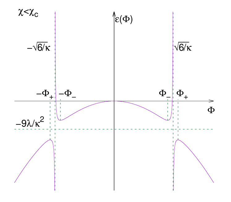
Figure 1: The energy density $\varepsilon$ as a function of $\Phi$ with $\Pi=0$ and given $\chi^{2}<\chi^{2}_{c}$. $\varepsilon(\Phi)$ has the ‘wine bottle’ (rather than the ‘Mexican hat’) shape, in particular it has minima at $\pm\Phi_{-}$, only in the domain $\Phi^{2}<6/\kappa$. The critical points $\pm\Phi_{+}$ are maxima of $\varepsilon$. If $\chi\rightarrow\chi_{c}$, then $\Phi_{0},\Phi_{\pm}\rightarrow\sqrt{6/\kappa}$ and $\varepsilon(\Phi_{\pm})\rightarrow-9\lambda/\kappa^{2}$, where $\pm\Phi_{0}$ are the two non-trivial zeros.

Summarizing the above results, we can give a qualitative picture on the behaviour of $\varepsilon$ as a function of $\Phi$ for $\Pi=0$ and for given $\chi$: First, suppose that $\chi^{2}<\chi^{2}_{c}$. Then, in the domain $\Phi<-\sqrt{6/\kappa}$, the energy density $\varepsilon$ is increasing from $-\infty$ to the local maximum $-\frac{1}{4}\lambda\Phi^{4}_{+}$ at $-\Phi_{+}$, and then it is decreasing and tends to $-\infty$ as $\Phi\rightarrow-\sqrt{6/\kappa}$. In the domain $-\sqrt{6/\kappa}<\Phi<\sqrt{6/\kappa}$, the energy density is decreasing from $+\infty$, at $-\Phi_{0}$ it has a zero, and it is decreasing further until $-\Phi_{-}$, where it takes its local minimum. Then it is increasing, takes its local maximum at $\Phi=0$, and then it is decreasing until the other local minimum at $\Phi_{-}$. Then, it is increasing again, taking the zero value at $\Phi_{0}$, and tends to $+\infty$ as $\Phi\rightarrow\sqrt{6/\kappa}$. Therefore, in this domain at fixed $\chi$, the graph of the function $\varepsilon=\varepsilon(\Phi,0,\chi)$ has the ‘wine bottle’ shape, i.e. it is like a ‘Mexican hat’, but the ‘brim’ of this ‘hat’ does not extend beyond $\Phi=\pm\sqrt{6/\kappa}$. In the domain $\sqrt{6/\kappa}<\Phi$, $\varepsilon$ is increasing from $-\infty$ to its local maximum at $\Phi_{+}$, and then decreasing back to $-\infty$ as $\Phi\rightarrow\infty$. The energy density has infinite discontinuities at $\mp\sqrt{6/\kappa}$.

If we increase $\chi^{2}$ to tend to $\chi^{2}_{c}$, then the local maximum in the domain $\Phi<-\sqrt{6/\kappa}$ and maximal value, and the local minimum in the domain $-\sqrt{6/\kappa}<\Phi<0$ and the corresponding minimal value tend, respectively, to $-\sqrt{6/\kappa}$ and $-9\lambda/\kappa^{2}$. Similarly, the local maximum in $\Phi>\sqrt{6/\kappa}$ and maximal value, and the local minimum in $0<\Phi<\sqrt{6/\kappa}$ and the minimal value tend, respectively, to $\sqrt{6/\kappa}$ and $-9\lambda/\kappa^{2}$. (Fig. 1)

If $\chi^{2}=\chi^{2}_{c}$, then $\varepsilon(\Phi,0,\chi_{c})=-\frac{3}{2}\frac{\lambda}{\kappa}\Phi^{2}$. Hence, along the $\chi^{2}=\chi^{2}_{c}$ line, the energy density and its derivatives are finite even at $\Phi=\pm\sqrt{6/\kappa}$ and changes smoothly and monotonically across $\Phi^{2}=6/\kappa$. (Fig. 2)

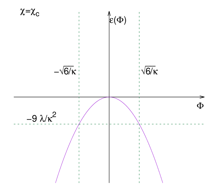
Figure 2: The energy density $\varepsilon$ as a function of $\Phi$ with $\Pi=0$ and $\chi^{2}=\chi^{2}_{c}$. $\varepsilon(\Phi)$ is not bounded from below.

Finally, suppose that $\chi^{2}>\chi^{2}_{c}$. Then, in the domain $\Phi<-\sqrt{6/\kappa}$, $\varepsilon$ is increasing from $-\infty$, takes the zero value at $-\Phi_{0}$, and it is increasing further and tends to $+\infty$ as $\Phi\rightarrow-\sqrt{6/\kappa}$. In the domain $-\sqrt{6/\kappa}<\Phi<\sqrt{6/\kappa}$, the energy density is increasing from $-\infty$, it takes its local maximum at $\Phi=0$, and then it is decreasing and tends to $-\infty$ as $\Phi\rightarrow\sqrt{6/\kappa}$. Thus, the graph of the function $\varepsilon=\varepsilon(\Phi,0,\chi)$ in this domain is a ‘simple hat’, whose ‘brim’ does not bend ‘upwards’ and does not extend beyond $\Phi=\pm\sqrt{6/\kappa}$. Finally, in the domain $\Phi>\sqrt{6/\kappa}$, $\varepsilon$ is decreasing from $+\infty$ to $-\infty$ and between these, at $\Phi_{0}$, it takes zero. The energy density has infinite discontinuities at $\mp\sqrt{6/\kappa}$. If we decrease $\chi^{2}$ to tend to $\chi^{2}_{c}$, then the zeros $\pm\Phi_{0}$ tend, respectively, to $\pm\sqrt{6/\kappa}$. (Fig. 3)

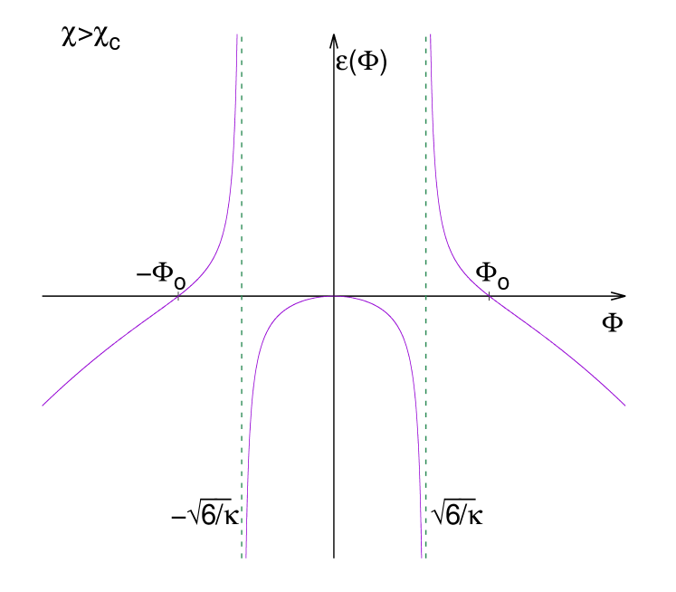
Figure 3: The energy density $\varepsilon$ as a function of $\Phi$ with $\Pi=0$ and given $\chi^{2}>\chi^{2}_{c}$. $\varepsilon(\Phi)$ is not bounded from below. If $\chi\rightarrow\chi_{c}$, then $\Phi_{0}\rightarrow\sqrt{6/\kappa}$.

The three disconnected parts of the graph of the function $\varepsilon=\varepsilon(\Phi,0,\chi)$ in the $\chi^{2}<\chi^{2}_{c}$ regime join smoothly to the corresponding parts in the $\chi^{2}>\chi^{2}_{c}$ regime, and, apart from the exceptional points at $(\Phi,\chi^{2})=(\pm\sqrt{6/\kappa},\chi^{2}_{c})$, they form three disconnected leaves. However, the ‘asymptotic ends’ of any of these leaves near the $\Phi=\pm\sqrt{6/\kappa}$ singularities behave oppositely in the two regimes. For example, the ‘wine bottle’ of the $\chi^{2}<\chi^{2}_{c}$ regime is continued in the ‘simple hat’ of the $\chi^{2}>\chi^{2}_{c}$ regime such that near the singularity $\Phi=-\sqrt{6/\kappa}$ the resulting leaf tends to $-\infty$ for $\chi^{2}>\chi^{2}_{c}$, but it tends to $+\infty$ for $\chi^{2}<\chi^{2}_{c}$.

Therefore, the $\Phi,\chi^{2}$–(half) plane is naturally split into six domains by the $\chi^{2}=\chi^{2}_{c}$ and $\Phi=\pm\sqrt{6/\kappa}$ lines, and it is only the domain $-\sqrt{6/\kappa}<\Phi<\sqrt{6/\kappa}$, $\chi^{2}<\chi^{2}_{c}$ where $\varepsilon$ has finite local minima. For fixed $\chi^{2}$ these minima are global, but the corresponding minimal value, $-\frac{1}{4}\lambda\Phi^{4}_{-}$, is decreasing and tends to the finite value $-9\lambda/\kappa^{2}$ as $\chi^{2}\rightarrow\chi^{2}_{c}$ (or, equivalently, as $\Phi^{2}_{-}\rightarrow 6/\kappa$). However, in this limit the second derivative $(\partial^{2}\varepsilon/\partial\Phi^{2})_{-}$, given by (3.38), tends to $+\infty$. On the other hand, as we saw above, if we consider the limit $\Phi\rightarrow-\sqrt{6/\kappa}$ along the line $\chi^{2}=\chi^{2}_{c}$, then $\varepsilon$ still tends to $-9\lambda/\kappa^{2}$, but $(\partial^{2}\varepsilon/\partial\Phi^{2})\rightarrow-3\lambda/\kappa$. Hence, there are special configurations with $|\Phi|^{2}=6/\kappa$ in which the energy-momentum tensor (2.5) is finite, but its derivatives are not; indicating that these configurations are probably unstable. Nevertheless, these provide the only ‘bridge’ between the $\Phi^{2}>6/\kappa$ and $\Phi^{2}<6/\kappa$ parts of the phase space.

Since, for given $\chi$, $(\partial\varepsilon/\partial\Pi)=0$ implies $\Pi=0$, the extremal points of $\varepsilon(\Phi,\Pi,\chi)$ with respect to $\Phi$ and $\Pi$ are just the extremal points of $\varepsilon(\Phi,0,\chi)$ with respect to $\Phi$. On the other hand, for $\Pi\not=0$ the domain of positivity of $\varepsilon$ changes: On the $\Phi,\chi^{2}$–(half) plane this domain is ‘wider’ for $\Pi^{2}>0$ than for $\Pi^{2}=0$, and, in particular, $\varepsilon$ is positive on a strip with the $\Phi=0$ center-line. In fact, for given $\chi^{2}$, in the $\Phi,\Pi^{2}$-(half) plane the domain on which $\varepsilon$ is non-positive is

$$\Pi^{2}+\Bigl{(}\sqrt{\frac{\lambda}{2}}\Phi^{2}+\sqrt{\frac{1}{2\lambda}}\bigl{(}\mu^{2}+\frac{1}{3}\Lambda-\frac{1}{9}\chi^{2}\bigr{)}\Bigr{)}^{2}\leq\frac{1}{2\lambda}\bigl{(}\mu^{2}+\frac{1}{3}\Lambda-\frac{1}{9}\chi^{2}\bigr{)}^{2}.$$

For given $\chi^{2}$ this domain is compact, but since the right hand side of this expression is never zero, this domain is not compact in the $\chi^{2}$–direction. Also, if $\Pi\not=0$, then the locus of the ‘bridge’ between the $\Phi^{2}>6/\kappa$ and $\Phi^{2}<6/\kappa$ parts of the phase space changes: It is given by the two hyperbolas $\chi^{2}-\frac{3}{2}\kappa\Pi^{2}=\chi^{2}_{c}$ in the $\Phi=\pm\sqrt{6/\kappa}$, $S={\rm const}$ 2-planes in the phase space. For a more detailed discussion of the behaviour of $\varepsilon$ see [10].

3.4.3 The static solution

It is an easy exercise to check that the equations (3.30)-(3.32) formally admit a static solution, which is just the Minkowski spacetime, but yield a condition for the numerical value of the constants $\lambda$, $\mu^{2}$, $\Lambda$ and $\kappa$ that is not satisfied in the observed Universe. In fact, $\Phi^{\bf i}=0$ solves (3.31) and yields $\Pi^{\bf i}=0$, and hence $\varepsilon=0$ and $P=0$. Then, by the second of (3.30), $\Lambda=0$ follows, which, by the first of (3.30), yields that $k=0$. Similarly, if $\Phi^{\bf i}$ is a non-zero static solution of (3.31), then $\Pi^{\bf i}=-\chi\Phi^{\bf i}/3$ and $|\Phi|^{2}=-(\mu^{2}+2\Lambda/3)/(\lambda+\kappa\mu^{2}/6)$. Substituting these into (3.32) and using the second of (3.30) we find that

$$|\Phi|^{2}=-\frac{\mu^{2}}{\lambda},\hskip 20.0pt\varepsilon=-\frac{\Lambda}{\kappa}=-\frac{1}{4}\lambda|\Phi|^{4}.$$

For $\lambda>0$ these imply that $\mu^{2}<0$ and $\Lambda>0$ must hold. Finally, by the first of (3.30) $k=0$ follows. It might be worth noting that this non-trivial static state of the Higgs field is precisely the symmetry breaking vacuum state that we saw in the Weinberg–Salam model, but clearly this is not a critical point of the energy density (3.32). In this static solution it would be a large positive value of the cosmological constant that compensates the large negative energy density of the Higgs vacuum. On the other hand, although the observed cosmological constant is strictly positive, but it is much-much smaller than that would follow from the Weinberg–Salam model via these expressions. In fact, in traditional units the energy density in the vacuum state would be $\varepsilon_{v}=-2.2\times 10^{46}erg/cm^{3}$, while that corresponding to the observed cosmological constant is $\varepsilon_{\Lambda}=4.7\times 10^{-11}erg/cm^{3}$. Thus, this static solution cannot be expected to give a reliable model of the observed Universe. That should be dynamical.

3.5 Example: Configurations with Kantowski–Sachs symmetries

In the present subsection we determine a class of field configurations that admit the isometries of the Kantowski–Sachs metrics as symmetries in which the (global or quasi-local) instantaneous vacuum states should be searched for. Since the number of spacetime symmetries is less than the maximal one, the Kantowski–Sachs case is technically more complicated than the FRW case. In subsection 3.5.1, we determine the matter field configurations that admit the Kantowski–Sachs symmetries, and then, in subsection 3.5.2, those with minimal energy density.

3.5.1 Matter fields with Kantowski–Sachs symmetries

Let us consider spacetimes with the Kantowski–Sachs line element $ds^{2}=dt^{2}-X^{2}dr^{2}-Y^{2}d\Omega^{2}$, where $X=X(t)$ and $Y=Y(t)$ are positive functions and $d\Omega^{2}$ denotes the line element on the unit 2-sphere (see e.g. [24, 25]). For example the line element inside the Schwarzschild black hole belongs to the Kantowski–Sachs class (see e.g. appendix B in [21]). These metrics admit four spacelike Killing vectors, the three familiar ones $K^{a}_{1}$, $K^{a}_{2}$ and $K^{a}_{3}$ for the spherical symmetry with transitivity surfaces $t={\rm const}$, $r={\rm const}$; and the fourth is $K^{a}_{4}=(\partial/\partial r)^{a}$, which commutes with the previous three. Let $v^{a}:=X^{-1}K^{a}_{4}$, the unit normal of the transitivity surfaces of the spherical symmetry in the $\Sigma_{t}:=\{t={\rm const}\}$ hypersurfaces. The extrinsic curvature of these hypersurfaces is $\chi_{ab}=-\dot{X}X^{-1}v_{a}v_{b}+\dot{Y}Y^{-1}q_{ab}$, where $q_{ab}$ is the induced (negative definite) metric on the $t={\rm const}$, $r={\rm const}$ 2-spheres and over-dot denotes derivative with respect to $t$. Note that $\chi=\chi(t)$, i.e. the mean curvature of the leaves $\Sigma_{t}$ is spatially constant. In the coordinates $(r,\theta,\phi)$ the only nonzero component of the curvature tensor of the intrinsic geometry of the hypersurfaces is ${\cal R}^{2}{}_{3cd}=-\sin^{2}\theta(\delta^{2}_{c}\delta^{3}_{d}-\delta^{2}_{d}\delta^{3}_{c})$; and hence the corresponding curvature scalar is ${\cal R}=2/Y^{2}>0$. A direct calculation shows that $D_{a}(\chi^{a}{}_{b}-\chi\delta^{a}_{b})=0$.

Recall that in field theory the vacuum states are defined to be those field configurations that (i.) do not break the spacetime symmetries and (ii.) minimize the energy functional. In particular, by the first requirement (a.) no state that can be a potential (instantaneous) vacuum state can specify any direction different from $v^{a}$; and (b.) any such state must be invariant (in some suitable sense) under the action of the spacetime symmetries. By (a.) the field strengths $E^{\alpha}_{a}$ and $B^{\alpha}_{ab}$, the Higgs field $\Phi^{\bf i}$ and a spinor multiplet $\psi^{r}_{A}$ in any particular vacuum state must be such that $E^{\alpha}_{a}=E^{\alpha}v_{a}$, $B^{\alpha}_{ab}=B^{\alpha}\varepsilon_{ab}$, $\mathbb{D}_{a}\Phi^{\bf i}=\varphi^{\bf i}v_{a}$ and $\psi^{r}_{A}=\psi^{r}\varepsilon_{A}$, where $E^{\alpha}$, $B^{\alpha}$, $\varphi^{\bf i}$ and $\psi^{r}$ are gauge covariant vector and spatial scalar fields, $\varepsilon_{ab}$ is the area 2-form on the $t={\rm const}$, $r={\rm const}$ 2-surfaces and $\varepsilon_{A}$ is one of the vectors of the normalized spinor dyad $\{o_{A},\iota_{A}\}$ adapted to the $t={\rm const}$, $r={\rm const}$ 2-surfaces (in the sense that $\sqrt{2}t_{a}=o_{A}\bar{o}_{A^{\prime}}+\iota_{A}\bar{\iota}_{A^{\prime}}$ and $\sqrt{2}v_{a}=o_{A}\bar{o}_{A^{\prime}}-\iota_{A}\bar{\iota}_{A^{\prime}}$). (To see that any spinor field of the spinor multiplet $\psi^{r}_{A}$ in the vacuum state must be proportional to either $o_{A}$ or $\iota_{A}$, it is enough to recall that the projections $P^{b}_{a}o_{B}\bar{o}_{B^{\prime}}$ and $P^{b}_{a}\iota_{B}\bar{\iota}_{B^{\prime}}$ are proportional to $v_{a}$, but for any nontrivial combination $\psi_{A}=-\psi_{0}\iota_{A}+\psi_{1}o_{A}$ the projection $P^{b}_{a}\psi_{B}\bar{\psi}_{B^{\prime}}$ is not.)

To formulate mathematically part (b.) of requirement (i.), let us recall how the spacetime symmetries are implemented in gauge theories (see [26]): In the actual system the state represented by a field configuration is said to be symmetric if for each Killing vector $K^{a}$ there exists a Lie algebra valued function $\lambda^{\alpha}g_{\alpha}$ such that

$${\pounds}_{K}E^{\alpha}_{a}=\lambda^{\mu}c^{\alpha}_{\mu\nu}E^{\nu}_{a},\hskip 10.0pt{\pounds}_{K}B^{\alpha}_{ab}=\lambda^{\mu}c^{\alpha}_{\mu\nu}B^{\nu}_{ab},$$

$${\pounds}_{K}\Phi^{\bf i}=\lambda^{\mu}T^{\bf i}_{\mu{\bf j}}\Phi^{\bf j},\hskip 10.0pt{\pounds}_{K}\Pi^{\bf i}=\lambda^{\mu}T^{\bf i}_{\mu{\bf j}}\Pi^{\bf j},\hskip 10.0pt{\pounds}_{K}\psi^{r}_{A}=\lambda^{\mu}T^{r}_{\mu{s}}\psi^{s}_{A};$$ (3.39)

i.e. it is required that the Lie dragging of the fields along the integral curves of the Killing vectors could always be compensated by an appropriate gauge transformation. Here ${\pounds}_{K}$ denotes Lie derivative along $K^{a}$, and actually the structure constants $c^{\alpha}_{\mu\nu}$ play the role of the representation matrices of the Lie algebra in the adjoint representation. Note that although the Lie derivative of a Weyl spinor field along a general vector field is not canonically defined, it is well defined if $K^{a}$ is a (conformal) Killing vector [27].

However, if a given field configuration is intended to represent a vacuum state, then it reduces the gauge group to the identity (symmetric vacuum) or to a non-trivial, smaller gauge group (symmetry breaking vacuum). In the latter case this subgroup is just the stabilizer subgroup $G_{v}\subset G$ of the vacuum state, and the Lie algebra valued function $\lambda^{\alpha}$ in the criteria (3.39) should be restricted to take its values in the Lie algebra of the reduced gauge group $G_{v}$. But then, just by the definition of $G_{v}$, the right hand sides of equations in (3.39) are all vanishing for such restricted Lie algebra valued functions. Thus

$${\pounds}_{K}E^{\alpha}_{a}=0,\hskip 10.0pt{\pounds}_{K}B^{\alpha}_{ab}=0,\hskip 10.0pt{\pounds}_{K}\Phi^{\bf i}=0,\hskip 10.0pt{\pounds}_{K}\Pi^{\bf i}=0,\hskip 10.0pt{\pounds}_{K}\psi^{r}_{A}=0$$ (3.40)

must hold for the fields in the vacuum states for any Killing vector $K^{a}$. Solving the first four of these equations is a straightforward exercise, and probably the simplest way of solving the fifth of these is based on the following observation: If the rotation Killing vectors are given explicitly by

$$K^{a}_{1}=-\sin\phi(\frac{\partial}{\partial\theta})^{a}-\cot\theta\cos\phi(\frac{\partial}{\partial\phi})^{a},\hskip 8.0ptK^{a}_{2}=\cos\phi(\frac{\partial}{\partial\theta})^{a}-\cot\theta\sin\phi(\frac{\partial}{\partial\phi})^{a},\hskip 8.0ptK^{a}_{3}=(\frac{\partial}{\partial\phi})^{a},$$

then the Lie derivative of the vectors of the normalized spin frame $\{o_{A},\iota_{A}\}$ is

$${\pounds}_{K_{l}}o_{A}=-\frac{\rm i}{2}Y_{l}o_{A},\hskip 20.0pt{\pounds}_{K_{l}}\iota_{A}=\frac{\rm i}{2}Y_{l}\iota_{A},\hskip 25.0ptl=1,2,3,4;$$

where $Y_{l}=(\sin\theta\sin\phi,\sin\theta\cos\phi,\cos\theta,0)$. (For the explicit form of the Lie derivative of spinors in terms of their covariant derivative and the Killing field, see [27].) Then, writing $\psi^{r}_{A}=\psi^{r}o_{A}$ or $\psi^{r}\iota_{A}$ (just according to the second paragraph of the present subsection) and substituting this into the fifth of (3.40), we find that $\psi^{r}=0$. Thus, the vacuum states of the EccSM system should be among the states represented by the field configurations of the form:

$$E^{\alpha}_{a}=E^{\alpha}(t)v_{a},\hskip 10.0ptB^{\alpha}_{ab}=B^{\alpha}(t)\varepsilon_{ab},\hskip 10.0pt\Phi^{\bf i}=\Phi^{\bf i}(t),\hskip 10.0pt\Pi^{\bf i}=\Pi^{\bf i}(t),\hskip 10.0pt\psi^{r}_{A}=0.$$ (3.41)

This structure of the magnetic field strength makes it possible to find a gauge in which $A^{\alpha}_{a}$ is also aligned with the spacetime symmetries. In fact, in the coordinate system $(t,r,\theta,\phi)$ the expression of the magnetic field strength $B^{\alpha}_{ab}=\partial_{a}A^{\alpha}_{b}-\partial_{b}A^{\alpha}_{a}+c^{\alpha}_{\mu\nu}A^{\mu}_{a}A^{\nu}_{b}$, together with $\sqrt{|q|}=Y^{2}(t)\sin\theta$, yields

$$\partial_{r}A^{\alpha}_{\theta}-\partial_{\theta}A^{\alpha}_{r}+c^{\alpha}_{\mu\nu}A^{\mu}_{r}A^{\nu}_{\theta}=0,$$

$$\partial_{r}A^{\alpha}_{\phi}-\partial_{\phi}A^{\alpha}_{r}+c^{\alpha}_{\mu\nu}A^{\mu}_{r}A^{\nu}_{\phi}=0,$$

$$\partial_{\theta}A^{\alpha}_{\phi}-\partial_{\phi}A^{\alpha}_{\theta}+c^{\alpha}_{\mu\nu}A^{\mu}_{\theta}A^{\nu}_{\phi}=B^{\alpha}Y^{2}\sin\theta.$$

The third of these equations decouples from the first two, and does not depend on $r$. Hence it can be solved for $A^{\alpha}_{\theta}$ and $A^{\alpha}_{\phi}$, and the solution can be chosen to be independent of $r$. (Their $t$-dependence cannot be chosen arbitrarily, that is determined by the evolution equations.) Then the first two of these equations form a system of partial differential equations for $A^{\alpha}_{r}$, whose integrability condition (using the third of these equations) is just $c^{\alpha}_{\mu\nu}B^{\mu}A^{\nu}_{r}=0$. Hence, by $\partial_{r}A^{\alpha}_{\theta}=\partial_{r}A^{\alpha}_{\phi}=0$, there is a gauge in which $v^{a}A^{\alpha}_{a}=0$ holds.

Finally, by the result for the form of $\mathbb{D}_{a}\Phi^{\bf i}$ (obtained in the second paragraph above) and the third of (3.41) we have that $v_{a}\varphi^{\bf i}=\mathbb{D}_{a}\Phi^{\bf i}=A^{\alpha}_{a}T^{\bf i}_{\alpha{\bf j}}\Phi^{\bf j}$. This implies, first, that the components $A^{\alpha}_{\theta}$ and $A^{\alpha}_{\phi}$ of the spatial vector potential take their values in the Lie algebra of the reduced gauge group $G_{v}$; and, second, that $\varphi^{\bf i}=0$ by $A^{\alpha}_{r}=0$, i.e.

$$\mathbb{D}_{a}\Phi^{\bf i}=0.$$ (3.42)

We search the instantaneous vacuum states among the field configurations satisfying (3.41)-(3.42), and we specify them in the next sections, where we evaluate requirement (ii.) above, too.

3.5.2 The minimal energy configurations

In the special field configurations (3.41)-(3.42), the energy density $\varepsilon$ of the matter fields (with the specific self-interaction term of the Weinberg–Salam model) reduces to

$$\varepsilon=\frac{1}{1-\frac{1}{6}\kappa|\Phi|^{2}}\Bigl{(}-\frac{1}{2}G_{\alpha\beta}\bigl{(}E^{\alpha}E^{\beta}+B^{\alpha}B^{\beta}\bigr{)}+\frac{1}{2}|\Pi|^{2}+\frac{1}{2}\bigl{(}\mu^{2}+\frac{1}{3}\Lambda-\frac{1}{9}\chi^{2}\bigr{)}|\Phi|^{2}+\frac{1}{4}\lambda|\Phi|^{4}\Bigr{)},$$ (3.43)

while the momentum density $\pi_{a}$ is zero. Thus, the matter sector of the (total or quasi-local) energy-momentum functional in these special configurations is simply the hypersurface integral of the (spatially constant) $\varepsilon$. Hence, to find the instantaneous vacuum states, we should determine the local minima of $\varepsilon$.

The structure of $\varepsilon=\varepsilon(E^{\alpha},B^{\alpha},\Phi^{\bf i},\Pi^{\bf i};\chi)$ is exactly the same that of $\varepsilon=\varepsilon(\Phi^{\bf i},\Pi^{\bf i};\chi)$ in the FRW case. Thus, they have the same qualitative properties that $\varepsilon=\varepsilon(\Phi,0;\chi)$ has for a single real scalar field $\Phi$. In particular, the critical points of $\varepsilon=\varepsilon(E^{\alpha},B^{\alpha},\Phi^{\bf i},\Pi^{\bf i};\chi)$ with respect to the matter field variables are at $E^{\alpha}=0$, $B^{\alpha}=0$, $\Pi^{\bf i}=0$ and $\Phi^{\bf i}$ solving (3.25). Its solutions have the pointwise norm (3.36), just like in the FRW case, whose reality is ensured precisely by the bound (3.37) for the mean curvature. It is only $\pm\Phi_{-}$ that represents local minima of the energy density.

4 The EccSM system with instantaneous vacuum states

4.1 The 3+1 form of the Lagrangian

Let the foliation $\Sigma_{t}$ of the spacetime be fixed, let $N$ be its lapse, and consider the so-called evolution vector field $\xi^{a}=Nt^{a}+N^{a}$, where $N^{a}$, the shift part of $\xi^{a}$, is tangent to $\Sigma_{t}$. The 3+1 form of the spacetime volume element is ${\rm d}v=N{\rm d}\Sigma{\rm d}t$, where, in a local coordinate system $(x^{1},x^{2},x^{3})$ on $\Sigma_{t}$, the hypersurface volume element is ${\rm d}\Sigma=\sqrt{|h|}{\rm d}^{3}x$. The time derivative of a spatial tensor field, say $T^{a...}_{b...}$, is defined by $\dot{T}^{a...}_{b...}:=({\pounds}_{\xi}T^{c...}_{d...})P^{a}_{c}\cdots P^{d}_{b}\cdots$. Thus, the Lagrangian variables in the Yang–Mills–Higgs sector are $\phi^{\alpha}$, $\dot{\phi}^{\alpha}$, $A^{\alpha}_{a}$, $\dot{A}^{\alpha}_{a}$, $\Phi^{\bf i}$ and $\dot{\Phi}^{\bf i}$. Since, however, the Lie derivative of a spinor field along a general vector field is not canonically defined, for the Lagrangian spinor field variables we choose the components $\psi^{r}_{\underline{A}\,}$ of the spinor field $\psi^{r}_{A}$ and their time derivative $\dot{\psi}^{r}_{\underline{A}\,}$, where the spinor components are defined with respect to some fixed normalized dual spinor basis $\{\varepsilon^{A}_{\underline{A}\,},\varepsilon^{\underline{A}\,}_{A}\}$ by $\psi^{r}_{A}=:\psi^{r}_{\underline{A}\,}\varepsilon^{\underline{A}\,}_{A}$.

Clearly, the form of the Lagrangian ${\cal L}_{I}$ and the potential $V$ remains the same in their 3+1 form, and it is straightforward to find the 3+1 form of ${\cal L}_{YM}$ and ${\cal L}_{W}$. The former is

$${\cal L}_{YM}=\frac{1}{2}G_{\alpha\beta}E^{\alpha}_{a}E^{\beta}_{b}h^{ab}+\frac{1}{4}G_{\alpha\beta}B^{\alpha}_{ac}B^{\beta}_{bd}h^{ab}h^{cd},$$ (4.1)

where by (3.4) the electric field strength is $E^{\alpha}_{a}=\frac{1}{N}(D_{a}(N\phi^{\alpha})+A^{\mu}_{a}c^{\alpha}_{\mu\nu}N\phi^{\nu}-\dot{A}^{\alpha}_{a}+{\pounds}_{N}A^{\alpha}_{a})$ and the magnetic field strength is expressed by the spatial vector potential and its derivative; and the latter is

$${\cal L}_{W}=\frac{\rm i}{2N}G_{rr^{\prime}}t^{AA^{\prime}}\Bigl{(}\!\!\!\! \bar{\psi}^{r^{\prime}}_{A^{\prime}}\varepsilon^{\underline{A}\,}_{A}\bigl{(}\dot{\psi}^{r}_{\underline{A}\,}-N^{e}D_{e}\psi^{r}_{\underline{A}\,}-Nt^{e}\Gamma^{\underline{B}\,}_{e{\underline{A}\,}}\psi^{r}_{\underline{B}\,}\bigr{)}-$$

$$-\!\!\!\! \psi^{r}_{A}\bar{\varepsilon}^{{\underline{A}\,}^{\prime}}_{A^{\prime}}\bigl{(}\dot{\bar{\psi}}^{r^{\prime}}_{{\underline{A}\,}^{\prime}}-N^{e}D_{e}\bar{\psi}^{r^{\prime}}_{{\underline{A}\,}^{\prime}}-Nt^{e}\bar{\Gamma}^{{\underline{B}\,}^{\prime}}_{e{\underline{A}\,}^{\prime}}\bar{\psi}^{r^{\prime}}_{{\underline{B}\,}^{\prime}}\bigr{)}\Bigr{)}+$$ (4.2)

$$+\frac{\rm i}{2}G_{rr^{\prime}}t^{AA^{\prime}}\phi^{\alpha}\bigl{(}\!\!\!\! T^{r}_{\alpha s}\psi^{s}_{A}\bar{\psi}^{r^{\prime}}_{A^{\prime}}-\bar{T}^{r^{\prime}}_{\alpha s^{\prime}}\bar{\psi}^{s^{\prime}}_{A^{\prime}}\psi^{r}_{A}\bigr{)}+\frac{\rm i}{2}G_{rr^{\prime}}h^{ab}\bigl{(}\bar{\psi}^{r^{\prime}}_{A^{\prime}}\mathbb{D}_{b}\psi^{r}_{A}-\psi^{r}_{A}\mathbb{D}_{b}\bar{\psi}^{r^{\prime}}_{A^{\prime}}\bigr{)},$$

where $\Gamma^{\underline{A}\,}_{e{\underline{B}\,}}:=\varepsilon^{\underline{A}\,}_{A}\nabla_{e}\varepsilon^{A}_{\underline{B}\,}$, and note that the spatial vector potential $A^{\alpha}_{a}$ is involved in $\mathbb{D}_{e}$. Thus, if we introduce the ‘mechanical’ Lagrangians $L_{YM}:=\int_{\Sigma}{\cal L}_{YM}N\sqrt{|h|}{\rm d}^{3}x$ and $L_{W}:=\int_{\Sigma}{\cal L}_{W}N\sqrt{|h|}{\rm d}^{3}x$, then for the canonical momenta we obtain

$$\frac{\delta L_{YM}}{\delta\dot{A}^{\alpha}_{a}}=-G_{\alpha\beta}E^{\beta}_{b}h^{ba},\hskip 20.0pt\frac{\delta L_{W}}{\delta\dot{\psi}^{r}_{\underline{A}\,}}=\frac{\rm i}{2}G_{rr^{\prime}}\bar{\psi}^{r^{\prime}}_{A^{\prime}}t^{A^{\prime}A}\varepsilon^{\underline{A}\,}_{A}.$$

Thus, as we claimed, $E^{\alpha}_{a}$ is essentially the momentum conjugate to $A^{\alpha}_{a}$, while the momentum conjugate to $\phi^{\alpha}$ is zero. The momentum conjugate to the spinor multiplet is just its own complex conjugate, in accordance with the fact that the field equations for the spinor fields are only first order.

On the other hand, because of the term $\frac{1}{12}R|\Phi|^{2}$ in ${\cal L}_{H}$, finding the most convenient 3+1 form of the Higgs Lagrangian is slightly more complicated. It is known [28] that the spacetime curvature scalar can be decomposed as

$$R={\cal R}+\chi_{ab}\chi^{ab}-\chi^{2}+\frac{2}{N\sqrt{|h|}}\frac{\rm d}{{\rm d}t}\bigl{(}\chi\sqrt{|h|}\bigr{)}+\frac{2}{N}D_{a}\bigl{(}D^{a}N-\chi N^{a}\bigr{)},$$

where ${\cal R}$ is the curvature scalar of the intrinsic geometry of the hypersurface; by means of which

$$R|\Phi|^{2}\!\!\!\! =\!\!\!\! \bigl{(}{\cal R}+\chi_{ab}\chi^{ab}-\chi^{2}\bigr{)}|\Phi|^{2}-\frac{2}{N}\chi\bigl{(}\dot{\Phi}^{\bf i}G_{\bf i\bf j^{\prime}}\bar{\Phi}^{\bf j^{\prime}}+\Phi^{\bf i}G_{\bf i\bf j^{\prime}}\dot{\bar{\Phi}}^{\bf j^{\prime}}\bigr{)}-\frac{2}{N}\bigl{(}D^{a}N-\chi N^{a}\bigr{)}D_{a}|\Phi|^{2}$$

$$+\!\!\!\! \frac{2}{N\sqrt{|h|}}\frac{\rm d}{{\rm d}t}\bigl{(}\chi|\Phi|^{2}\sqrt{|h|}\bigr{)}+\frac{2}{N}D_{a}\bigl{(}(D^{a}N-\chi N^{a})|\Phi|^{2}\bigr{)}.$$

Thus, in the 3+1 form of the Higgs Lagrangian, it seems natural to drop the last two terms, which, after integration, would give a total time derivative and the integral of a total spatial divergence, respectively. Hence, we choose the 3+1 form of the Higgs Lagrangian to be

$$\hat{\cal L}_{H}:\!\!\!\! =\!\!\!\! \frac{1}{2}G_{\bf i\bf j^{\prime}}t^{a}\bigl{(}{\nabla\!\!\!\!/}_{a}\Phi^{\bf i}\bigr{)}t^{b}\bigl{(}{\nabla\!\!\!\!/}_{b}\bar{\Phi}^{\bf j^{\prime}}\bigr{)}+\frac{1}{2}G_{\bf i\bf j^{\prime}}h^{ab}\bigl{(}D_{a}\Phi^{\bf i}+A^{\alpha}_{a}T^{\bf i}_{\alpha{\bf k}}\Phi^{\bf k}\bigr{)}\bigl{(}D_{b}\bar{\Phi}^{\bf j^{\prime}}+A^{\beta}_{b}\bar{T}^{\bf j^{\prime}}_{\beta{\bf l^{\prime}}}\bar{\Phi}^{\bf l^{\prime}}\bigr{)}-$$ (4.3)

$$-\!\!\!\! \frac{1}{4}G_{\bf i\bf j\bf k^{\prime}\bf l^{\prime}}\Phi^{\bf i}\Phi^{\bf j}\bar{\Phi}^{\bf k^{\prime}}\bar{\Phi}^{\bf l^{\prime}}-\frac{1}{12}\bigl{(}{\cal R}+\chi_{ab}\chi^{ab}-\chi^{2}\bigr{)}G_{\bf i\bf j^{\prime}}\Phi^{\bf i}\bar{\Phi}^{\bf j^{\prime}}+$$

$$+\!\!\!\! \frac{1}{6}\frac{1}{N}\chi G_{\bf i\bf j^{\prime}}\bigl{(}\dot{\Phi}^{\bf i}\bar{\Phi}^{\bf j^{\prime}}+\Phi^{\bf i}\dot{\bar{\Phi}}^{\bf j^{\prime}}\bigr{)}+\frac{1}{6}\frac{1}{N}\bigl{(}D^{a}N-\chi N^{a}\bigr{)}D_{a}|\Phi|^{2},$$

where

$$t^{a}{\nabla\!\!\!\!/}_{a}\Phi^{\bf i}=\frac{1}{N}\bigl{(}\dot{\Phi}^{\bf i}+N\phi^{\alpha}T^{\bf i}_{\alpha{\bf k}}\Phi^{\bf j}-N^{a}D_{a}\Phi^{\bf i}\bigr{)}.$$ (4.4)

The canonical momentum conjugate to $\Phi^{\bf i}$, calculated from the ‘mechanical’ Lagrangian $\hat{L}_{H}:=\int_{\Sigma}\hat{\cal L}_{H}N\sqrt{|h|}{\rm d}^{3}x$, is

$$\frac{\delta\hat{L}_{H}}{\delta\dot{\Phi}^{\bf i}}=\frac{1}{2}G_{\bf i\bf j^{\prime}}\bigl{(}t^{a}{\nabla\!\!\!\!/}_{a}\bar{\Phi}^{\bf j^{\prime}}+\frac{1}{3}\chi\bar{\Phi}^{\bf j^{\prime}}\bigr{)}=\frac{1}{2}G_{\bf i\bf j^{\prime}}\bar{\Pi}^{\bf j^{\prime}}.$$ (4.5)

Therefore, $\Pi^{\bf i}=t^{a}{\nabla\!\!\!\!/}_{a}\Phi^{\bf i}+\frac{1}{3}\chi\Phi^{\bf i}$ is, in fact, essentially the canonical momentum conjugate to $\bar{\Phi}^{\bf i^{\prime}}$, as we claimed in subsection 3.2.

4.2 The instantaneous vacuum states

4.2.1 The definition of the instantaneous vacuum states

We search for the instantaneous vacuum states among the critical points of ${\tt Q}[K]$. In these states the gauge fields and the spinor fields are vanishing, and the Higgs field $\Phi^{\bf i}_{v}$ is such that $D_{e}\Phi^{\bf i}_{v}=0$, it solves (3.23), and its canonical momentum is zero: $\Pi^{\bf i}_{v}=0$. By (4.4) the last condition is equivalent to

$$\frac{1}{N}\dot{\Phi}^{\bf i}_{v}=\frac{1}{N}\bigl{(}\dot{\Phi}^{\bf i}_{v}-N^{a}D_{a}\Phi^{\bf i}_{v}\bigr{)}=t^{e}(\nabla_{e}\Phi^{\bf i}_{v})=t^{e}({\nabla\!\!\!\!/}_{e}\Phi^{\bf i}_{v})=\Pi^{\bf i}_{v}-\frac{1}{3}\chi\Phi^{\bf i}_{v}=-\frac{1}{3}\chi\Phi^{\bf i}_{v}.$$ (4.6)

Here we used also that the scalar and spatial vector potentials, $\phi^{\alpha}$ and $A^{\alpha}_{a}$, can be chosen to be vanishing even globally.

At the end of subsection 3.3.2 we saw that the 1-parameter family of these states does not solve all of the field equations. Nevertheless, we want these instantaneous states to be physical states, thus they are required to solve the constraint parts of the field equations. Thus, an instantaneous vacuum state is represented not only by a special configuration of the matter fields alone, but by such a configuration of the matter fields and the initial data set for Einstein’s equations. As we saw, in the gravitational part of such a data both the mean curvature and the intrinsic curvature scalar must be constant.

Moreover, if the spacetime admits some geometric symmetry, then it seems natural to require that the instantaneous vacuum states be represented by field configurations with the same geometric symmetry. Or, in other words, these states could be expected to break only the internal gauge symmetries, but not the geometric symmetries of the spacetime. In particular, if the spacetime admits the FRW or Kantowski–Sachs symmetries, then one could expect that the instantaneous vacuum states have the same geometric symmetries, too. In this case, the (spatially constant) mean curvature in the gravitational part of the vacuum state, which plays the role of the extrinsic York time parameter and labels the hypersurfaces, is identical with the mean curvature of the actual hypersurface on which e.g. the rest mass of the matter fields is calculated.

4.2.2 The existence of the instantaneous vacuum states: A condition on the mean curvature

For the usual self-interaction coefficient of the Higgs field, $G_{\bf i\bf j\bf k^{\prime}\bf l^{\prime}}=\lambda G_{\bf k^{\prime}(\bf i}G_{\bf j)\bf l^{\prime}}$, the norm of the ‘vacuum value’ of the Higgs field (see equation (3.26)) is

$$|\Phi_{v}|^{2}=\frac{6}{\kappa}\Bigl{(}1-\sqrt{1+\frac{\kappa}{3\lambda}\bigl{(}\mu^{2}+\frac{1}{3}\Lambda-\frac{1}{9}\chi^{2}\bigr{)}}\Bigr{)}=-\frac{\mu^{2}}{\lambda}+\frac{\kappa}{12}\frac{\mu^{4}}{\lambda^{2}}-\frac{1}{\lambda}\Bigl{(}\frac{\Lambda}{3}-\frac{1}{9}\chi^{2}\Bigr{)}+...,$$ (4.7)

just the solution $\Phi^{2}_{-}$ given by (3.36). (The solution with the $+$ sign in front of the square root is a local maximum rather than a minimum of the energy density in the domain $|\Phi|^{2}\geq 6/\kappa$, see subsection 3.4.2.) Thus the structure of $|\Phi_{v}|^{2}$ (and the interpretation of the various corrections in $|\Phi_{v}|^{2}$ to the flat-spacetime Standard Model expression) is very similar to that of (2.23). The only (but essential) difference between these two is the extrinsic curvature term in (4.7), which makes the instantaneous vacuum states time dependent.

However, for given parameters $\lambda$, $\mu^{2}$ and $\Lambda$ the inequality (3.37) is a nontrivial condition on $\chi^{2}$, i.e. on the mean curvature of the hypersurface $\Sigma_{t}$ on which instantaneous vacuum states are possible. This is a finite upper bound, and its value is given by $\chi^{2}_{c}:=9(3\lambda/\kappa+\mu^{2}+\Lambda/3)\simeq 4.8\times 10^{64}cm^{-2}$. On hypersurfaces with greater mean curvature there are no such vacuum states at all. The corresponding characteristic (Hubble) time is $t_{c}:=3/\chi_{c}\simeq 4.5\times 10^{-43}sec$, which is almost ten times longer than the Planck time $T_{P}\simeq 5.39\times 10^{-44}sec$.

In particular, in a FRW spacetime the instantaneous vacuum states start to emerge on the hypersurface for which the Hubble time $t_{H}:=S/\dot{S}$ was $t_{c}$. The present value of the Hubble constant in our observed Universe is $H_{0}:=(\dot{S}/S)_{\rm now}=\frac{1}{3}\chi_{\rm now}\simeq 7\times 10^{-28}cm^{-1}$. Hence, the condition (3.37) is satisfied in the present epoch of the evolution of the Universe. On the other hand, in all the asymptotic power series solutions of the field equations of the EccH system with a Small Bang singularity, in a vicinity of the singularity the mean curvature of the $t={\rm const}$ hypersurfaces does exceed $\chi_{c}$ [10]. Also, in all of these solutions in which $|\Phi|^{2}$ takes $6/\kappa$ at regular spacetime points, the mean curvature either exceeds $\chi_{c}$ in a vicinity of, or takes the value $\chi_{c}$ at the $|\Phi|^{2}=6/\kappa$ hypersurface. Therefore, in both cases there is a regime in the spacetime where instantaneous vacuum states do not exist.

Similarly, since the mean curvature e.g. on the standard foliation of the interior Schwarzschild solution diverges as $\sim t^{-3/2}$, inequality (3.37) is a non-trivial condition in Kantowski–Sachs spacetimes, too: Near the spacetime singularity, deeply behind the black hole horizon, instantaneous vacuum states do not exist.

On the other hand, note that by the specific form of the energy density in the FRW and Kantowski–Sachs cases, given, respectively, by (3.32) and (3.43), the instantaneous vacuum states, when they exist, are gauge symmetry breaking vacuum states. In the presence of these geometric symmetries the energy density does not have any gauge symmetric stable minimum.

4.2.3 The existence of the instantaneous vacuum states: A condition on the geometric symmetries

Since the instantaneous vacuum states are expected to be physical states, they must solve the Hamiltonian constraint. Hence, by (3.28), the corresponding curvature scalar ${\cal R}_{v}$ must be negative. Therefore, globally defined instantaneous vacuum states exist only when the hypersurface $\Sigma_{t}$ admits hyperboloidal 3-geometries and the group of spacetime symmetries is compatible with ${\cal R}_{v}<0$. In particular, in the presence of FRW symmetries, $k$ in (3.30) must be $-1$. Thus, to have global instantaneous vacuum states the Universe must be open.

In Kantowski–Sachs spacetimes, by $E^{\alpha}_{a}=0$, $B^{\alpha}_{ab}=0$, $\psi^{r}_{A}=0$ and $\mathbb{D}_{a}\Phi^{\bf i}=0$ the only constraint in the matter sector, the Gauss constraint, is satisfied. Remarkably enough, although a priori we allowed the matter field variables to have special direction dependence, i.e. to be aligned with the distinguished vector field $v^{a}$, in the spacetime-symmetric minimal energy states the matter field configurations turn out to be isotropic. This result is compatible with the general structure of the critical configurations of the general energy-momentum functional obtained in 3.3.2. Since $D_{a}(\chi^{a}{}_{b}-\chi\delta^{a}_{b})=0$ holds by the results of the first paragraph of subsection 3.5.1 and the momentum density built from the Kantowski–Sachs invariant fields of the EccSM model is vanishing, the momentum constraint of General Relativity is identically satisfied. On the other hand, the Hamiltonian constraint, written in the form

$${\cal R}-(\chi_{ab}-\frac{1}{3}\chi h_{ab})(\chi^{ab}-\frac{1}{3}\chi h^{ab})=2\Lambda+2\kappa\varepsilon-\frac{2}{3}\chi^{2},$$

is a non-trivial condition on the difference of the spatial curvature scalar and the square of the trace-free part of the extrinsic curvature. Although the matter field variables in the instantaneous vacuum states must be isotropic on $\Sigma_{t}$, apparently the extrinsic curvature need not. Nevertheless, the general analysis of the critical configurations of the energy-momentum functional in subsection 3.3.2 shows that the extrinsic curvature must be a constant pure trace (see equation (3.27)). Otherwise the field configuration would not be critical with respect to general variations, though they are with respect to variations in the Kantowski–Sachs class.

With this additional restriction coming from the results of the general analysis in subsection 3.3.2, in the instantaneous vacuum states, the mean curvature $\chi$ determines the spatial curvature scalar on $\Sigma_{t}$ completely via equation (4.7) and the Hamiltonian constraint:

$$\frac{1}{2}{\cal R}_{v}=\Lambda-\frac{1}{4}\kappa\lambda|\Phi_{v}|^{4}-\frac{1}{3}\chi^{2}=\frac{1}{1-\frac{1}{12}\kappa|\Phi_{v}|^{2}}\bigl{(}\Lambda+\frac{1}{4}\kappa\mu^{2}|\Phi_{v}|^{2}-\frac{1}{3}\chi^{2}\bigr{)}.$$ (4.8)

Here, in the second equality, we used (3.25). However, by (4.7), the first two terms together in the brackets on the right is negative for any $\chi^{2}\leq\chi^{2}_{c}$, and hence the curvature scalar ${\cal R}_{v}$ must be negative, while, according to the first paragraph of subsection 3.5.1, the curvature scalar on any Kantowski–Sachs symmetric 3-space is strictly positive. Therefore, global instantaneous vacuum states whose matter and gravitational sectors would be Kantowski–Sachs invariant do not exist.

On the other hand, if the vacuum states are not required to admit the same symmetries that the spacetime has, i.e. if they are allowed to be $SO(1,3)$-symmetric even in the $k=1,0$ FRW or Kantowski–Sachs spacetimes, too, then the instantaneous vacuum states can be defined at least on open subsets of the $t={\rm const}$ hypersurfaces, i.e. they can exist quasi-locally. In particular, in the $k=0$ FRW spacetime the instantaneous vacuum states can exist globally, but in the $k=1$ case only on proper subsets of $\Sigma_{t}\approx S^{3}$.

Similarly, in the Kantowski–Sachs case, if we require the 3-metric in the gravitational sector of the vacuum state to be $O(1,3)$-invariant (rather than to belong to the Kantowski–Sachs class with isometry group $\mathbb{R}\times O(3)$), just like the matter fields and the extrinsic curvature, then that should be the hyperboloidal metric $dh_{v}^{2}=-\frac{K^{2}}{K^{2}+\rho^{2}}d\rho^{2}-\rho^{2}d\Omega^{2}$ on some domain $r>\ln\rho_{0}$ of the 3-manifold $\Sigma_{t}\approx\mathbb{R}\times S^{2}$ with $\rho_{0}>0$, where the radial coordinate is $\rho:=\exp(r)-\rho_{0}$, $K^{2}:=-6/{\cal R}_{v}$, and the 2-sphere $r=\ln\rho_{0}$ corresponds to the (missing) origin of the hyperboloidal space. Clearly, this quasi-locally defined instantaneous vacuum state on the given open subset of $\Sigma_{t}$ exists if the mean curvature $\chi$ satisfies the strict inequality in (3.37), in which case it is determined completely by the mean curvature.

4.3 The genesis/evanescence and time dependence of the rest masses

Following the general ideas in [5], now we calculate the rest mass of the fields of the EccSM system via the BEH mechanism in nearly FRW and Kantowski–Sachs spacetime: We assume that the spacetime satisfies those conditions that ensure the existence of instantaneous vacuum states. In particular, it should admit a foliation by constant mean curvature hypersurfaces $\Sigma_{t}$, whose mean curvature $\chi$ can be used as an external time variable (the so-called York time).

However, as we saw in subsection 4.2 (and showed explicitly in the FRW case), the existence of local minima of the spatially constant energy density, and hence the existence of the instantaneous vacuum states, is guaranteed only on the spacelike hypersurfaces with mean curvature smaller than $\chi_{c}$. Moreover, if the instantaneous vacuum states exist, then they are necessarily gauge symmetry breaking states. The existence of the bound $\chi_{c}$ yields a non-trivial ‘genesis’/‘evanescence’ of the rest masses of certain fields of the standard model, depending on whether $\chi$ is decreasing or increasing when $\chi$ takes the critical value $\chi_{c}$. Also, the electromagnetic interaction (together with the electric charge) emerges from the $U(2)$ gauge theory in the Weinberg–Salam model as an ‘effective’ gauge theory only in the presence of the (global or quasi-local) instantaneous gauge symmetry breaking vacuum states (see [5]). Thus, the hypersurface whose mean curvature is just the bound $\chi_{c}$ is the ‘moment of genesis/evanescence’ of the (globally or quasi-locally defined) electric charge, too.

Thus let us suppose that $\chi^{2}<\chi^{2}_{c}$, and let us fix a particular (gauge symmetry breaking) vacuum state $\Phi^{\bf i}_{v}$. Then, in the unitary gauge (see [5, 22], or subsection 2.6.1), the independent Lagrangian field variables of the matter sector are $\phi^{\alpha}$, $A^{\alpha}_{a}$, $\psi^{r}_{A}$, $H^{\bf i}:=\Phi^{\bf i}-\Phi^{\bf i}_{v}$ and the corresponding velocities; and the vacuum states correspond to the vanishing of these variables. The mass of the various fields can be read off from the second derivative of the Lagrangian with respect to $\phi^{\alpha}$, $A^{\alpha}_{a}$, $H^{\bf i}$ and $\psi^{r}_{A}$ at the vacuum state, provided its first derivatives are vanishing. Denoting the 3+1 form of the matter Lagrangian density by $\hat{\cal L}$ (which is just ${\cal L}$ in which ${\cal L}_{H}$ is replaced by $\hat{\cal L}_{H}$), these first derivatives with respect to the gauge potentials at the vacuum states are

$$\bigl{(}\frac{\partial\hat{\cal L}}{\partial\phi^{\alpha}}\bigr{)}_{v}=\bigl{(}\frac{\partial\hat{\cal L}_{H}}{\partial\phi^{\alpha}}\bigr{)}_{v}=-\frac{1}{6}\chi\bigl{(}G_{\bf i\bf k^{\prime}}\bar{T}^{\bf k^{\prime}}_{\alpha{\bf j^{\prime}}}+G_{\bf j^{\prime}\bf k}T^{\bf k}_{\alpha{\bf i}}\bigr{)}\Phi^{\bf i}_{v}\bar{\Phi}^{\bf j^{\prime}}_{v}=0,$$

$$\bigl{(}\frac{\partial\hat{\cal L}}{\partial A^{\alpha}_{a}}\bigr{)}_{v}=\bigl{(}\frac{\partial\hat{\cal L}_{H}}{\partial A^{\alpha}_{a}}\bigr{)}_{v}=\frac{1}{2}G_{\bf i\bf j^{\prime}}\Bigl{(}\bigl{(}D^{a}\bar{\Phi}^{\bf j^{\prime}}_{v}\bigr{)}T^{\bf i}_{\alpha{\bf k}}\Phi^{\bf k}_{v}+\bigl{(}D^{a}\Phi^{\bf i}_{v}\bigr{)}\bar{T}^{\bf j^{\prime}}_{\alpha{\bf l^{\prime}}}\bar{\Phi}^{\bf l^{\prime}}_{v}\Bigr{)}=0.$$

Here, in the first of these, we used (4.6) and the gauge invariance of the fiber metric $G_{\bf i\bf j^{\prime}}$; and, in the second, we used $D_{a}\Phi^{\bf i}_{v}=0$ and $A^{\alpha}_{e}=0$. These two can be summarized as $(\partial\hat{\cal L}/\partial\omega^{\alpha}_{a})_{v}=((\partial\hat{\cal L}/\partial\phi^{\alpha})t^{a}+(\partial\hat{\cal L}/\partial A^{\alpha}_{b})P^{a}_{b})=0$, and hence the mass matrix for the gauge fields,

$$M^{2}_{\alpha\beta}:=\frac{1}{4}\bigl{(}g_{ab}\frac{\partial^{2}\hat{\cal L}}{\partial\omega^{\alpha}_{a}\partial\omega^{\beta}_{b}}\bigr{)}_{v}=\frac{1}{2}\Bigl{(}\bigl{(}T^{\bf i}_{\alpha{\bf k}}\Phi^{\bf k}_{v}\bigr{)}G_{\bf i\bf j^{\prime}}\bigl{(}\bar{T}^{\bf j^{\prime}}_{\beta{\bf l^{\prime}}}\bar{\Phi}^{\bf l^{\prime}}_{v}\bigr{)}+\bigl{(}T^{\bf i}_{\beta{\bf k}}\Phi^{\bf k}_{v}\bigr{)}G_{\bf i\bf j^{\prime}}\bigl{(}\bar{T}^{\bf j^{\prime}}_{\alpha{\bf l^{\prime}}}\bar{\Phi}^{\bf l^{\prime}}_{v}\bigr{)}\Bigr{)},$$ (4.9)

is a well defined real, symmetric and positive semi-definite matrix. The first derivative of $\hat{\cal L}$ with respect to the spinor field $\psi^{r}_{A}$ at the vacuum state is also zero (by $\psi^{r}_{A}=0$), and the corresponding mass matrix is

$$M_{rs}:=-\frac{1}{2}\bigl{(}\epsilon_{\underline{A}\,\underline{B}\,}\frac{\partial^{2}\hat{\cal L}}{\partial\psi^{r}_{\underline{A}\,}\partial\psi^{s}_{\underline{B}\,}}\bigr{)}_{v}={\rm i}Y_{rs{\bf i^{\prime}}}\bar{\Phi}^{\bf i^{\prime}}_{v},$$ (4.10)

just the component of the Yukawa coupling determined by the Higgs field in the vacuum state, $\Phi^{\bf i}_{v}$. (Here $\epsilon_{\underline{A}\,\underline{B}\,}$ is the anti-symmetric Levi-Civita symbol.) The first derivative of $\hat{\cal L}$ with respect to $H^{\bf i}$ is

$$\bigl{(}\frac{\partial\hat{\cal L}}{\partial H^{\bf i}}\bigr{)}_{v}\!\!\!\! =\!\!\!\! \bigl{(}\frac{\partial(\hat{\cal L}_{H}-V)}{\partial H^{\bf i}}\bigr{)}_{v}=-\frac{1}{18}\chi^{2}G_{\bf i\bf j^{\prime}}\bar{\Phi}^{\bf j^{\prime}}_{v}-\frac{1}{2}\Bigl{(}\frac{1}{6}\bigl{(}{\cal R}_{v}+\chi^{ab}\chi_{ab}-\chi^{2}\bigr{)}+\mu^{2}\Bigr{)}G_{\bf i\bf j^{\prime}}\bar{\Phi}^{\bf j^{\prime}}_{v}$$

$$-\!\!\!\! \frac{1}{2}G_{\bf i\bf j\bf k^{\prime}\bf l^{\prime}}\Phi^{\bf j}_{v}\bar{\Phi}^{\bf k^{\prime}}_{v}\bar{\Phi}^{\bf l^{\prime}}_{v}=$$

$$=\!\!\!\! -\frac{1}{2}\Bigl{(}\frac{1}{3}\kappa\varepsilon_{v}+\mu^{2}+\frac{1}{3}\Lambda-\frac{1}{9}\chi^{2}\Bigr{)}G_{\bf i\bf j^{\prime}}\bar{\Phi}^{\bf j^{\prime}}_{v}-\frac{1}{2}G_{\bf i\bf j\bf k^{\prime}\bf l^{\prime}}\Phi^{\bf j}_{v}\bar{\Phi}^{\bf k^{\prime}}_{v}\bar{\Phi}^{\bf l^{\prime}}_{v}=0.$$

Here ${\cal R}_{v}$ and $\varepsilon_{v}$ denote the spatial curvature scalar and energy density in the vacuum state $\Phi^{\bf i}_{v}$, respectively; and first we used $\phi^{\alpha}=0$, $A^{\alpha}_{e}=0$, $D_{a}\Phi^{\bf i}_{v}=0$ and (4.6), and then the Hamiltonian constraint, (3.27) and (3.23). Therefore, in contrast to the spacetime vacuum states of subsection 2.6.1, the instantaneous gauge symmetry breaking vacuum states are critical points of the Lagrangian. Hence, its second derivatives at these states,

$$M^{2}_{\bf i\bf j^{\prime}}:=-\bigl{(}\frac{\partial^{2}\hat{\cal L}}{\partial H^{\bf i}\partial\bar{H}^{\bf j^{\prime}}}\bigr{)}_{v}\!\!\!\! =\!\!\!\! \Bigl{(}\frac{1}{6}\kappa\varepsilon_{v}+\frac{1}{6}\Lambda+\frac{1}{2}\mu^{2}-\frac{1}{9}\chi^{2}\Bigr{)}G_{\bf i\bf j^{\prime}}+G_{\bf i\bf k\bf j^{\prime}\bf l^{\prime}}\Phi^{\bf k}_{v}\bar{\Phi}^{\bf l^{\prime}}_{v},$$ (4.11)

$$M^{2}_{\bf i\bf j}:=-\bigl{(}\frac{\partial^{2}\hat{\cal L}}{\partial H^{\bf i}\partial H^{\bf j}}\bigr{)}_{v}\!\!\!\! =\!\!\!\! \frac{1}{2}G_{\bf i\bf j\bf k^{\prime}\bf l^{\prime}}\bar{\Phi}^{\bf k^{\prime}}_{v}\bar{\Phi}^{\bf l^{\prime}}_{v},$$ (4.12)

are well defined. Note that, even if the instantaneous vacuum state were only a quasi-local one (in the $k=1,0$ FRW and Kantowski–Sachs cases), these mass matrices would still be well defined and independent of the parameter $\rho_{0}$ fixing the domain of the hyperboloidal line element $dh_{v}^{2}$ (see the end of subsection 4.2.3). Because of the extrinsic curvature term in (3.36), the instantaneous gauge symmetry breaking vacuum states are in general time dependent, and hence the mass matrices are also time dependent.

In the Einstein–conformally coupled Weinberg–Salam model, $\Phi^{\bf i}_{v}$ is chosen to have the form $(0,|\Phi_{v}|)$ (as a column vector), and $H^{\bf i}=(0,H)$ for some real function $H$. Then by (2.12) and (4.10) the rest mass of the electron is $m_{e}=\frac{1}{\sqrt{2}}G_{e}|\Phi_{v}|$, and the neutrino is massless. Evaluating the mass matrix for the gauge fields in (4.9) and recalling that in particle physics the gauge fields are defined to be the connection 1-forms divided by the corresponding coupling constants (see the footnote to subsection 2.1), we find that the fields $Z_{e}:=\frac{1}{\sqrt{g^{2}+g^{\prime}{}^{2}}}(\omega^{0}_{e}-\omega^{3}_{e})$ and $W^{\pm}_{e}:=\frac{1}{g\sqrt{2}}(\omega^{1}_{e}\mp{\rm i}\omega^{2}_{e})$ get the masses $\frac{1}{2}\sqrt{g^{2}+g^{\prime}{}^{2}}|\Phi_{v}|$ and $\frac{1}{2}g|\Phi_{v}|$, respectively, but $\varpi_{e}:=\frac{1}{gg^{\prime}\sqrt{g^{2}+g^{\prime}{}^{2}}}(g^{2}\omega^{0}_{e}+g^{\prime}{}^{2}\omega^{3}_{e})$, identified with the photon field, is massless. Thus, the mass of the gauge bosons and the electron is given by the corresponding expression in the Weinberg–Salam model except that the vacuum value $v=\sqrt{-\mu^{2}/\lambda}$ is replaced by $|\Phi_{v}|$, whose expansion is $v(1+\Lambda/3\mu^{2}-\chi^{2}/9\mu^{2}-\kappa\mu^{2}/12\lambda+...)^{1/2}$. The mass of the real Higgs field $H$ is

$$m^{2}_{H}:\!\!\!\! =\!\!\!\! -\bigl{(}\frac{\partial^{2}\hat{\cal L}}{\partial H^{2}}\bigr{)}_{v}=|\Phi_{v}|^{-2}\Bigl{(}M^{2}_{\bf i\bf j}\Phi^{\bf i}_{v}\Phi^{\bf j}_{v}+2M^{2}_{\bf i\bf j^{\prime}}\Phi^{\bf i}_{v}\bar{\Phi}^{\bf j^{\prime}}_{v}+\bar{M}^{2}_{\bf i^{\prime}\bf j^{\prime}}\bar{\Phi}^{\bf i^{\prime}}_{v}\bar{\Phi}^{\bf j^{\prime}}_{v}\Bigr{)}=$$ (4.13)

$$=\!\!\!\! \lambda|\Phi_{v}|^{2}+2|\Phi_{v}|^{-2}M^{2}_{\bf i\bf j^{\prime}}\Phi^{\bf i}_{v}\bar{\Phi}^{\bf j^{\prime}}_{v}=2\lambda|\Phi_{v}|^{2}-\frac{1}{9}\chi^{2},$$

where, to evaluate (4.11), we used (3.25). Because of the extra mean curvature term $\chi^{2}/9$ on the right, the time dependence of the Higgs and the other fields is slightly different: e.g. $m^{2}_{e}/m^{2}_{H}$ depends on $\chi$.

If in a FRW spacetime $\chi^{2}=\chi^{2}_{c}$ (at $4.5\times 10^{-43}sec$ Hubble time), then the vacuum value of the Higgs field is $|\Phi_{v}|^{2}=6/\kappa$. Hence, at the instant of genesis, the mass e.g. of the electrons was $\simeq 6\times 10^{26}cm^{-1}$. By (4.7) this decreased to its half by $5.9\times 10^{-43}sec$ Hubble time. The electron mass decreased to twice its present value (i.e. to $2\times(2.6\times 10^{10}cm^{-1})$) by $4.5\times 10^{-27}sec$ Hubble time. The Higgs mass at the moment of genesis was $1.3\times 10^{32}cm^{-1}$. This decreased to its half by $5.8\times 10^{-43}sec$ Hubble time, and decreased to twice of its present value, $2\times(6.2\times 10^{15}cm^{-1})$, by $5.5\times 10^{-26}sec$ Hubble time. The characteristic time scale of the weak interactions, i.e. that the Higgs mass parameter defines, is $1/c|\mu|\simeq 5.4\times 10^{-27}sec$. Thus, even at this time scale the mass of both the Higgs and the other particles were approximately twice bigger than their present value. The rest mass of matter fields falling into a spherical black hole behaves in the opposite way: The (quasi-locally defined) rest mass of the electron, the $W^{\pm}$ and $Z$ gauge bosons and the Higgs field is increasing until the instant corresponding to the critical value $\chi_{c}$ of the mean curvature, and then the masses evanesce just before hitting the central singularity.

Finally, rewriting the Lagrangian ${\cal L}_{W}$ in terms of the fields $W^{\pm}_{e}$, $Z_{e}$ and $\varpi_{e}$ (as e.g. in [5]), for the charge of the electron we obtain exactly that in the Weinberg–Salam model. It does not depend on the York time.

5 Summary and final remarks

We investigated certain kinematical consequences of the conformally invariant coupling of the Higgs field of the Standard Model to Einstein’s theory of gravity. First, we showed that spacetime vacuum states, i.e. which would have maximal spacetime symmetry, solve the field equations and minimize the energy density, do not exist. Then, we showed that in the $k=1,0$ FRW and the Kantowski–Sachs spacetimes (hence, in particular, in spherical black holes) global instantaneous vacuum states, i.e. field configurations on the transitivity hypersurfaces of the spacetime symmetries which would be invariant with respect to the spacetime symmetries, solve the constraint parts of the field equations and minimize the energy functional, do not exist. Also, general quasi-local (i.e. not necessarily global) instantaneous vacuum states do not exist on hypersurfaces whose mean curvature is greater than a large, but finite critical value. If the mean curvature is less than this critical value, then instantaneous vacuum states exist, which, as we saw in the FRW and Kantowski–Sachs cases, are necessarily gauge symmetry breaking states.

Using this concept of the global or quasi-local instantaneous (gauge symmetry breaking) vacuum states, we determined how the rest mass of the fields of the Standard Model depends on the extrinsic York time parameter of the hypersurfaces. We found that there are extreme gravitational situations in which the notion of rest mass, zero or non-zero, of the Higgs field cannot be introduced at all, and the BEH mechanism does not work. In these situations the fields do not have particle interpretation. If they have, then the non-zero rest masses, introduced via the BEH mechanism, are time dependent in a non-stationary spacetime. Also, in the absence of the vacuum states above, electromagnetism and electric charge do not emerge from the Standard Model.

The time dependence (and the different time dependence) of the Higgs and the other particles is significant only when the mean curvature is close to its critical value. Thus, it may have a potential significance in the particle physics processes in the very early Universe, or near the central singularity in black holes. Hence it could be interesting to see whether or not this time dependence, and in particular the fact that at the characteristic time scale of the weak interactions the rest masses were twice their present value, could yield observable effect in the particle genesis era of the very early Universe.

If the mean curvature of the hypersurfaces happened to be increasing and exceeded the critical value, then the massive fields of the Standard Model would lose their rest mass. In our (asymptotically exponentially expanding) Universe the mean curvature asymptotically tends to the finite, constant value $\sqrt{\Lambda/3}$. Hence the ‘reverse–BEH’ mechanism at the cosmological scale cannot provide the way in which the fields lose their rest mass (as it would be desirable in the CCC model). The ‘reverse-BEH’ mechanism takes place inside black holes, deeply behind the event horizon near the central singularity.

6 Appendix: The total variation of the Lagrangian for Weyl spinor fields

Let $\{E^{a}_{\underline{a}\,},\vartheta^{\underline{a}\,}_{a}\}$, ${\underline{a}\,}=0,...,3$, be a $g_{ab}$-orthonormal dual frame field and $\{\varepsilon^{A}_{\underline{A}\,},\varepsilon^{\underline{A}\,}_{A}\}$, ${\underline{A}\,}=0,1$, the corresponding normalized dual spinor basis, i.e. for which $E^{a}_{{\underline{A}\,}{\underline{A}\,}^{\prime}}:=E^{a}_{\underline{a}\,}\sigma^{\underline{a}\,}_{{\underline{A}\,}{\underline{A}\,}^{\prime}}=\varepsilon^{A}_{\underline{A}\,}\bar{\varepsilon}^{A^{\prime}}_{{\underline{A}\,}^{\prime}}$ holds, where $\sigma^{\underline{a}\,}_{{\underline{A}\,}{\underline{A}\,}^{\prime}}$ are the $SL(2,\mathbb{C})$ Pauli matrices (including the factor $1/\sqrt{2}$). If $\Gamma^{\underline{A}\,}_{e{\underline{B}\,}}:=\varepsilon^{\underline{A}\,}_{A}\nabla_{e}\varepsilon^{A}_{\underline{B}\,}$, the spacetime connection 1-form in the spinor basis above, then the Lagrangian for a multiplet of Weyl spinor fields, $\psi^{r}_{A}$, is

$${\cal L}_{W}\!\!\!\! =\!\!\!\! \frac{\rm i}{2}G_{rr^{\prime}}g^{ab}\bigl{(}\bar{\psi}^{r^{\prime}}_{A^{\prime}}{\nabla\!\!\!\!/}_{b}\psi^{r}_{A}-\psi^{r}_{A}{\nabla\!\!\!\!/}_{b}\bar{\psi}^{r^{\prime}}_{A^{\prime}}\bigr{)}=$$ (6.1)

$$=\!\!\!\! \frac{\rm i}{2}G_{rr^{\prime}}\epsilon^{\underline{A}\,\underline{B}\,}\epsilon^{{\underline{A}\,}^{\prime}{\underline{B}\,}^{\prime}}E^{b}_{{\underline{B}\,}{\underline{B}\,}^{\prime}}\Bigl{(}\bar{\psi}^{r^{\prime}}_{{\underline{A}\,}^{\prime}}\bigl{(}\partial_{b}\psi^{r}_{\underline{A}\,}-\psi^{r}_{\underline{D}\,}\Gamma^{\underline{D}\,}_{b{\underline{A}\,}}+\omega^{\alpha}_{b}T^{r}_{\alpha s}\psi^{s}_{\underline{A}\,}\bigr{)}-$$

$$-\psi^{r}_{\underline{A}\,}\bigl{(}\partial_{b}\bar{\psi}^{r^{\prime}}_{{\underline{A}\,}^{\prime}}-\bar{\psi}^{r^{\prime}}_{{\underline{D}\,}^{\prime}}\bar{\Gamma}^{{\underline{D}\,}^{\prime}}_{b{\underline{A}\,}^{\prime}}+\omega^{\alpha}_{b}\bar{T}^{r^{\prime}}_{\alpha s^{\prime}}\bar{\psi}^{s^{\prime}}_{{\underline{A}\,}^{\prime}}\bigr{)}\Bigr{)},$$

where $\epsilon^{\underline{A}\,\underline{B}\,}$ is the anti-symmetric Levi-Civita symbol and $\partial_{b}$ denotes the gradient acting on functions. If $E^{a}_{\underline{a}\,}(u)$, $\psi^{r}_{\underline{A}\,}(u)$ are arbitrary smooth 1-parameter families of tetrads and spinor components, respectively, such that $E^{a}_{\underline{a}\,}(0)=E^{a}_{\underline{a}\,}$ and $\psi^{r}_{\underline{A}\,}(0)=\psi^{r}_{\underline{A}\,}$, and $\delta$ denotes the derivative with respect to $u$ at $u=0$, then by (6.1)

$$\delta{\cal L}_{W}\!\!\!\! =\!\!\!\! \frac{\rm i}{2}G_{rr^{\prime}}\epsilon^{\underline{A}\,\underline{B}\,}\epsilon^{{\underline{A}\,}^{\prime}{\underline{B}\,}^{\prime}}\delta E^{b}_{{\underline{B}\,}{\underline{B}\,}^{\prime}}\Bigl{(}\bar{\varepsilon}^{A^{\prime}}_{{\underline{A}\,}^{\prime}}\bar{\psi}^{r^{\prime}}_{A^{\prime}}\varepsilon^{A}_{\underline{A}\,}{\nabla\!\!\!\!/}_{b}\psi^{r}_{A}-\varepsilon^{A}_{\underline{A}\,}\psi^{r}_{A}\bar{\varepsilon}^{A^{\prime}}_{{\underline{A}\,}^{\prime}}{\nabla\!\!\!\!/}_{b}\bar{\psi}^{r^{\prime}}_{A^{\prime}}\Bigr{)}+$$ (6.2)

$$+\frac{\rm i}{2}G_{rr^{\prime}}\epsilon^{\underline{A}\,\underline{B}\,}\epsilon^{{\underline{A}\,}^{\prime}{\underline{B}\,}^{\prime}}E^{b}_{{\underline{B}\,}{\underline{B}\,}^{\prime}}\Bigl{(}\delta\bar{\psi}^{r^{\prime}}_{{\underline{A}\,}^{\prime}}\varepsilon^{A}_{\underline{A}\,}{\nabla\!\!\!\!/}_{b}\psi^{r}_{A}-\delta\psi^{r}_{\underline{A}\,}\varepsilon^{A^{\prime}}_{{\underline{A}\,}^{\prime}}{\nabla\!\!\!\!/}_{b}\bar{\psi}^{r^{\prime}}_{A^{\prime}}\Bigr{)}+$$

$$+\frac{\rm i}{2}G_{rr^{\prime}}\epsilon^{\underline{A}\,\underline{B}\,}\epsilon^{{\underline{A}\,}^{\prime}{\underline{B}\,}^{\prime}}E^{b}_{{\underline{B}\,}{\underline{B}\,}^{\prime}}\Bigl{(}\bar{\varepsilon}^{A^{\prime}}_{{\underline{A}\,}^{\prime}}\bar{\psi}^{r^{\prime}}_{A^{\prime}}\varepsilon^{A}_{\underline{A}\,}{\nabla\!\!\!\!/}_{b}\bigl{(}\varepsilon^{\underline{D}\,}_{A}\delta\psi^{r}_{\underline{D}\,}\bigr{)}-\varepsilon^{A}_{\underline{A}\,}\psi^{r}_{\underline{A}\,}\bar{\varepsilon}^{A^{\prime}}_{{\underline{A}\,}^{\prime}}{\nabla\!\!\!\!/}_{b}\bigl{(}\bar{\varepsilon}^{{\underline{D}\,}^{\prime}}_{A^{\prime}}\delta\bar{\psi}^{r^{\prime}}_{{\underline{D}\,}^{\prime}}\bigr{)}\Bigr{)}-$$

$$-\frac{\rm i}{2}\epsilon^{\underline{A}\,\underline{B}\,}\epsilon^{{\underline{A}\,}^{\prime}{\underline{B}\,}^{\prime}}E^{b}_{{\underline{B}\,}{\underline{B}\,}^{\prime}}\Bigl{(}\delta^{{\underline{D}\,}^{\prime}}_{{\underline{A}\,}^{\prime}}\delta\Gamma^{\underline{D}\,}_{b{\underline{A}\,}}-\delta^{\underline{D}\,}_{\underline{A}\,}\delta\bar{\Gamma}^{{\underline{D}\,}^{\prime}}_{b{\underline{A}\,}^{\prime}}\Bigr{)}G_{rr^{\prime}}\psi^{r}_{\underline{D}\,}\bar{\psi}^{r^{\prime}}_{{\underline{D}\,}^{\prime}}=$$

$$=\!\!\!\! \frac{\rm i}{2}G_{rr^{\prime}}g^{ab}{\nabla\!\!\!\!/}_{b}\Bigl{(}\bar{\psi}^{r^{\prime}}_{A^{\prime}}\varepsilon_{A}^{\underline{A}\,}\delta\psi^{r}_{\underline{A}\,}-\psi^{r}_{A}\bar{\varepsilon}_{A^{\prime}}^{{\underline{A}\,}^{\prime}}\delta\bar{\psi}^{r^{\prime}}_{{\underline{A}\,}^{\prime}}\Bigr{)}-$$

$$-{\rm i}G_{rr^{\prime}}\Bigl{(}\varepsilon^{A^{\prime}B^{\prime}}\bar{\varepsilon}^{B^{\prime}}_{{\underline{B}\,}^{\prime}}\delta\bar{\psi}^{r^{\prime}}_{{\underline{B}\,}^{\prime}}\bigl{(}{\nabla\!\!\!\!/}_{A^{\prime}}{}^{A}\psi^{r}_{A}\bigr{)}-\varepsilon^{AB}\varepsilon^{\underline{B}\,}_{B}\delta\psi^{r}_{\underline{B}\,}\bigl{(}{\nabla\!\!\!\!/}_{A}{}^{A^{\prime}}\bar{\psi}^{r^{\prime}}_{A^{\prime}}\bigr{)}\Bigr{)}+$$

$$+\frac{\rm i}{2}\delta E^{b}_{\underline{b}\,}E^{a}_{\underline{a}\,}\eta^{\underline{b}\,\underline{a}\,}G_{rr^{\prime}}\Bigl{(}\bar{\psi}^{r^{\prime}}_{A^{\prime}}{\nabla\!\!\!\!/}_{b}\psi^{r}_{A}-\psi^{r}_{A}{\nabla\!\!\!\!/}_{b}\bar{\psi}^{r^{\prime}}_{A^{\prime}}\Bigr{)}-$$

$$-\frac{\rm i}{2}\epsilon^{\underline{A}\,\underline{B}\,}\epsilon^{{\underline{A}\,}^{\prime}{\underline{B}\,}^{\prime}}E^{b}_{{\underline{B}\,}{\underline{B}\,}^{\prime}}\Bigl{(}\delta^{{\underline{D}\,}^{\prime}}_{{\underline{A}\,}^{\prime}}\delta\Gamma^{\underline{D}\,}_{b{\underline{A}\,}}-\delta^{\underline{D}\,}_{\underline{A}\,}\delta\bar{\Gamma}^{{\underline{D}\,}^{\prime}}_{b{\underline{A}\,}^{\prime}}\Bigr{)}G_{rr^{\prime}}\psi^{r}_{\underline{D}\,}\bar{\psi}^{r^{\prime}}_{{\underline{D}\,}^{\prime}}.$$

Thus, the second term on the right yields the field equations, while the variation of the tetrad field in the third term can be written as

$$\delta E^{b}_{\underline{b}\,}E^{a}_{\underline{a}\,}\eta^{\underline{b}\,\underline{a}\,}=\delta E^{(b}_{\underline{b}\,}E^{a)}_{\underline{a}\,}\eta^{\underline{b}\,\underline{a}\,}+\delta E^{[b}_{\underline{b}\,}E^{a]}_{\underline{a}\,}\eta^{\underline{b}\,\underline{a}\,}=\frac{1}{2}\delta g^{ab}+\varepsilon^{BA}\bar{\lambda}^{A^{\prime}B^{\prime}}+\varepsilon^{B^{\prime}A^{\prime}}\lambda^{AB},$$ (6.3)

where $\lambda^{AB}=\lambda^{(AB)}$ is defined to be the anti-self-dual part of the anti-symmetric part $\delta E^{[b}_{\underline{b}\,}E^{a]}_{\underline{a}\,}\eta^{\underline{b}\,\underline{a}\,}$ of the variation of the tetrad field. To evaluate the last term in (6.2), we need the explicit form of the variation of the spinor connection 1-form. Since

$$\Gamma^{\underline{A}\,}_{e{\underline{B}\,}}=\frac{1}{2}\sigma^{{\underline{A}\,}{\underline{A}\,}^{\prime}}_{\underline{a}\,}\sigma^{\underline{b}\,}_{{\underline{B}\,}{\underline{A}\,}^{\prime}}\vartheta^{\underline{a}\,}_{a}\nabla_{e}E^{a}_{\underline{b}\,}=:\frac{1}{2}\sigma^{{\underline{A}\,}{\underline{A}\,}^{\prime}}_{\underline{a}\,}\sigma^{\underline{b}\,}_{{\underline{B}\,}{\underline{A}\,}^{\prime}}\gamma^{\underline{a}\,}_{e{\underline{b}\,}},$$

we should compute the variation of the connection 1-form $\gamma^{\underline{a}\,}_{e{\underline{b}\,}}$ in the linear frame bundle. It is

$$\delta\gamma^{\underline{a}\,}_{e{\underline{b}\,}}\!\!\!\! =\!\!\!\! \delta\vartheta^{\underline{a}\,}_{a}\nabla_{e}E^{a}_{\underline{b}\,}+\vartheta^{\underline{a}\,}_{a}\frac{1}{2}g^{ac}\bigl{(}-\nabla_{c}\delta g_{eb}+\nabla_{e}\delta g_{cb}+\nabla_{b}\delta g_{ec}\bigr{)}E^{b}_{\underline{b}\,}+\vartheta^{\underline{a}\,}_{a}\nabla_{e}\bigl{(}\delta E^{a}_{\underline{b}\,}\bigr{)}=$$

$$=\!\!\!\! \vartheta^{\underline{a}\,}_{a}\nabla_{e}\bigl{(}\delta E^{[a}_{\underline{m}\,}E^{b]}_{\underline{n}\,}\eta^{\underline{m}\,\underline{n}\,}\bigr{)}\vartheta^{\underline{c}\,}_{b}\eta_{\underline{c}\,\underline{b}\,}+\frac{1}{2}\vartheta^{\underline{a}\,}_{a}\Bigl{(}g^{ac}\bigl{(}\nabla_{c}\delta g^{fd}\bigr{)}g_{fe}g_{db}-\bigl{(}\nabla_{b}\delta g^{af}\bigr{)}g_{fe}\Bigr{)}E^{b}_{\underline{b}\,}.$$

Substituting this into the last term of (6.2) and using (6.3), by forming total divergences we obtain that

$$\delta{\cal L}_{W}\!\!\!\! =\!\!\!\! \frac{\rm i}{2}\nabla^{a}\Bigl{(}G_{rr^{\prime}}\bar{\psi}^{r^{\prime}}_{A^{\prime}}\varepsilon^{\underline{A}\,}_{A}\bigl{(}\delta\psi^{r}_{\underline{A}\,}+\lambda_{\underline{A}\,}{}^{\underline{B}\,}\psi^{r}_{\underline{B}\,}\bigr{)}-G_{rr^{\prime}}\psi^{r}_{A}\bar{\varepsilon}^{{\underline{A}\,}^{\prime}}_{A^{\prime}}\bigl{(}\delta\bar{\psi}^{r^{\prime}}_{{\underline{A}\,}^{\prime}}+\bar{\lambda}_{{\underline{A}\,}^{\prime}}{}^{{\underline{B}\,}^{\prime}}\bar{\psi}^{r^{\prime}}_{{\underline{B}\,}^{\prime}}\bigr{)}\Bigr{)}-$$ (6.4)

$$-{\rm i}G_{rr^{\prime}}\Bigl{(}\bigl{(}\delta\psi^{r}_{\underline{A}\,}+\lambda_{\underline{A}\,}{}^{\underline{B}\,}\psi^{r}_{\underline{B}\,}\bigr{)}\varepsilon^{\underline{A}\,}_{A}\bigl{(}{\nabla\!\!\!\!/}^{AA^{\prime}}\bar{\psi}^{r^{\prime}}_{A^{\prime}}\bigr{)}-\bigl{(}\delta\bar{\psi}^{r^{\prime}}_{{\underline{A}\,}^{\prime}}+\bar{\lambda}_{{\underline{A}\,}^{\prime}}{}^{{\underline{B}\,}^{\prime}}\bar{\psi}^{r^{\prime}}_{{\underline{B}\,}^{\prime}}\bigr{)}\bar{\varepsilon}^{{\underline{A}\,}^{\prime}}_{A^{\prime}}\bigl{(}{\nabla\!\!\!\!/}^{A^{\prime}A}\psi^{r}_{A}\bigr{)}\Bigr{)}+$$

$$+\frac{\rm i}{8}G_{rr^{\prime}}\Bigl{(}\bar{\psi}^{r^{\prime}}_{A^{\prime}}{\nabla\!\!\!\!/}_{BB^{\prime}}\psi^{r}_{A}+\bar{\psi}^{r^{\prime}}_{B^{\prime}}{\nabla\!\!\!\!/}_{AA^{\prime}}\psi^{r}_{B}-\psi^{r}_{A}{\nabla\!\!\!\!/}_{BB^{\prime}}\bar{\psi}^{r^{\prime}}_{A^{\prime}}-\psi^{r}_{B}{\nabla\!\!\!\!/}_{AA^{\prime}}\bar{\psi}^{r^{\prime}}_{B^{\prime}}\Bigr{)}\delta g^{ab},$$

where $\lambda_{\underline{A}\,}{}^{\underline{B}\,}:=\varepsilon^{A}_{\underline{A}\,}\lambda_{A}{}^{B}\varepsilon^{\underline{B}\,}_{B}$, the components of $\lambda_{A}{}^{B}$ in the spinor basis.

To see the meaning of the combination $\delta\psi^{r}_{\underline{A}\,}+\lambda_{\underline{A}\,}{}^{\underline{B}\,}\psi^{r}_{\underline{B}\,}$, let us consider a 1-parameter family of spinor dual bases $\{\varepsilon^{A}_{\underline{A}\,}(u),\varepsilon^{\underline{A}\,}_{A}(u)\}$ in the spinor bundle in which $\{\varepsilon^{A}_{\underline{A}\,}(0),\varepsilon^{\underline{A}\,}_{A}(0)\}=\{\varepsilon^{A}_{\underline{A}\,},\varepsilon^{\underline{A}\,}_{A}\}$ is a normalized dual spinor dyad. Then the variation of the spinor basis is

$$\delta\varepsilon^{\underline{A}\,}_{A}\!\!\!\! =\!\!\!\! -\varepsilon^{\underline{A}\,}_{B}\bigl{(}\delta\varepsilon^{B}_{\underline{B}\,}\bigr{)}\varepsilon^{\underline{B}\,}_{A}=\varepsilon^{\underline{A}\,}_{B}\bigl{(}\delta\varepsilon^{(B}_{\underline{B}\,}\bigr{)}\varepsilon^{C)}_{\underline{C}\,}\epsilon^{\underline{B}\,\underline{C}\,}\varepsilon_{CA}-\frac{1}{2}\varepsilon^{\underline{A}\,}_{A}\varepsilon_{BC}\bigl{(}\delta\varepsilon^{B}_{\underline{B}\,}\bigr{)}\varepsilon^{C}_{\underline{C}\,}\epsilon^{\underline{B}\,\underline{C}\,}=$$

$$=\!\!\!\! \varepsilon^{\underline{A}\,}_{B}\lambda^{B}{}_{A}-\frac{1}{2}\omega\varepsilon^{\underline{A}\,}_{A}=\lambda^{\underline{A}\,}{}_{\underline{B}\,}\varepsilon^{\underline{B}\,}_{A}-\frac{1}{2}\omega\varepsilon^{\underline{A}\,}_{A},$$

where $\lambda^{AB}$ is just the anti-self-dual part of the variation of the corresponding tetrad field in (6.3), while $\omega$ is defined to be $\varepsilon_{BC}\bigl{(}\delta\varepsilon^{B}_{\underline{B}\,}\bigr{)}\varepsilon^{C}_{\underline{C}\,}\epsilon^{\underline{B}\,\underline{C}\,}$. Thus $\lambda^{\underline{A}\,}{}_{\underline{B}\,}$ represents the infinitesimal $SL(2,\mathbb{C})$ transformation of the spinor dyad, while $\omega$ an (in general complex) infinitesimal conformal rescaling of the symplectic spinor metric. In fact, the variation of the corresponding spinor and spacetime metrics, respectively, are $\delta\varepsilon^{AB}=\omega\varepsilon^{AB}$, and hence $\delta g^{ab}=(\omega+\bar{\omega})g^{ab}$. Nevertheless, as Penrose showed [29], complex conformal rescalings of the symplectic spinor metric yields torsion. Since we keep the variation of the spin frame within the framework of Einstein’s general relativity, $\omega$ must be real. Therefore, $\omega=\frac{1}{2}\varepsilon_{AB}\delta\varepsilon^{AB}=\frac{1}{8}g_{ab}\delta g^{ab}$ represents an infinitesimal genuine (real conformal) change of the metric, while $\lambda^{A}{}_{B}$ is only a pure gauge transformation. Thus, finally, suppose that $\omega=0$ and consider the transformation of the components $\psi^{r}_{\underline{A}\,}$ of the spinor field $\psi^{r}_{A}$ under such a variation of the spinor basis. It is $\delta\psi^{r}_{\underline{A}\,}=-\lambda_{\underline{A}\,}{}^{\underline{B}\,}\psi^{r}_{\underline{B}\,}$. Hence, the combination $\delta\psi^{r}_{\underline{A}\,}+\lambda_{\underline{A}\,}{}^{\underline{B}\,}\psi^{r}_{\underline{B}\,}$ represents, in fact, the variation of the spinor field components up to pure $SL(2,\mathbb{C})$ basis transformations, i.e. up to gauge. Hence, the second line of (6.4) contributes to the field equation (2.8), while the third line to the energy-momentum tensor (2.3) of the spinor fields.

The author is grateful to Árpád Lukács, Péter Vecsernyés and György Wolf for the numerous and enlightening discussions both on the structure of the Standard Model and on various aspects of the present suggestion. Special thanks to György Wolf for the careful reading of the draft of the paper, his suggestions to improve the text at several points and for drawing the figures.

References

- [1] R. Penrose, M. A. H. MacCallum, Twistor theory: An approach to the quantisation of fields and space-time, Phys. Rep. 6 241-316 (1972), doi:10.1016/0370-1573(73)90008-2
- [2] R. Penrose, The Road to Reality, A Complete Guide to the Laws of the Universe, Jonathan Cape, London 2004, ISBN 0-224-04447-8
- [3] P. W. Higgs, Broken symmetries and the masses of gauge bosons, Phys. Rev. Lett. 13 508-509 (1964), doi: 10.1103/PhysRevLett.13.508
- [4] F. Englert, R. Brout, Broken symmetry and the mass of gauge vector mesons, Phys. Rev. Lett. 13 321-323 (1964), doi: 10.1103/PhysRevLett.13.321
- [5] E. S. Abers, B. W. Lee, Gauge theories, Phys. Rep. 9 1–141 (1973), doi: 10.1016/0370-1573(73)90027-6
- [6] T.-P. Cheng, L.-F. Li, Gauge Theory of Elementary Particle Physics, Clarendon Press, Oxford 1984, ISBN 0-19-851961-3
- [7] R. Penrose, Cycles of Time, The Bodley Head, London 2010, ISBN 9780224080361
- [8] R. Penrose, W. Rindler, Spinors and Spacetime, vol 1, Cambridge University Press, Cambridge 1982, ISBN 0-521-24527-3
- [9] R. Penrose, W. Rindler, Spinors and Spacetime, vol 2, Cambridge University Press, Cambridge 1986, ISBN 0-521-252671-9
- [10] L. B. Szabados, Gy. Wolf, Singularities in Einstein–conformally coupled Higgs cosmological models, arXiv: 1802.00774 [gr-qc]
- [11] E. T. Newman, R. Penrose, New conservation laws for zero rest-mass fields in asymptotically flat spacetimes, Proc. Roy. Soc. A 305 175-204 (1968), doi: 10.1098/rspa.1968.0112
- [12] L. B. Szabados, Quasi-local energy-momentum and angular momentum in GR, Living Rev. Relativity 12 (2009) 4, http://www.livingreviews.org/ lrr-2009-4, doi: 10.12942/lrr-2009-4
- [13] R. Arnowitt, S. Deser, C. W. Misner, The dynamics of general relativity, in Gravitation: An Introduction to Current Research, pp. 227–265, Ed.: Witten, L., Wiley, New York, London, 1962, ISBN 0124366406, arXiv: gr-qc/0405109
- [14] H. Bondi, M. G. J. van der Burg, A. W. K. Metzner, Gravitational waves in general relativity. VII. Waves from axi-symmetric isolated systems, Proc. R. Soc. London, Ser. A 269 21-52 (1962), doi: 10.1098/rspa.1962.0161 R. K. Sachs, Asymptotic symmetries in gravitational theory, Phys. Rev. 128 2851–2864 (1962), doi: 10.1103/PhysRev.128.2851 A. R. Exton, E. T. Newman, R. Penrose, Conserved quantities in the Einstein–Maxwell theory, J. Math. Phys. 10 1566–1570 (1969), doi: 10.1063/1.1665006
- [15] G. Abbott, S. Deser, Stability of gravity with a cosmological constant, Nucl. Phys. B 195 76-96 (1982), doi: 10.1016/0550-3213(82)90049-9
- [16] L. B. Szabados, P. Tod, A positive Bondi-type mass in asymptotically de Sitter spacetimes, Class. Quantum Grav. 32 (2015) 205011, doi: 10.1088/0264-9381/32/20/205011, arXiv: 1505.06637 [gr-qc]
- [17] L. B. Szabados, Mass, gauge conditions and spectral properties of the Sen–Witten and 3-surface twistor operators in closed universes, Class. Quantum Grav. 29 095001 (2012), doi: 10.1088/0264-9381/29/9/095001, arXiv: 1112.2966 [gr-qc]
- [18] L. B. Szabados, On the total mass of closed universes with a positive cosmological constant, Class. Quantum Grav. 30 165013 (2013), doi: 10.1088/0264-9381/30/16/165013, arXiv: 1306.3863 [gr-qc]
- [19] A. J. Dougan, L. J. Mason, Quasilocal mass constructions with positive energy, Phys. Rev. Lett. 67 2119-2122 (1991), doi: 10.1103/PhysRevLett.67.2119
- [20] L. B. Szabados, On the positivity of the quasi-local mass, Class. Quantum Grav. 10 1899-1905 (1993), doi: 10.1088/0264-9381/10/9/027
- [21] S. W. Hawking, G. F. R. Ellis, The Large Scale Structure of Spacetime, Cambridge University Press, Cambridge 1973, ISBN 0-521-09906-4
- [22] S. Weinberg, General theory of broken local symmetry, Phys. Rev. D 7 1068-1082 (1973), doi: 10.1103/PhysRevD.7.1068
- [23] R. M. Wald, General Relativity, University of Chicago Press, Chicago 1984, ISBN 0-226-87033-2
- [24] C. B. Collins, Global structure of the “Kantowski–Sachs” cosmological models, J. Math. Phys. 18 2116-2124 (1977), doi: 10.1063/1.523191
- [25] M. A. H. MacCallum, Anisotropic and inhomogeneous relativistic cosmologies, in General Relativity, An Einstein centenary survey, Eds. W. Israel, S. W. Hawking, Cambridge University Press, Cambridge 1979, ISBN 0-521-22285-0
- [26] P. Forgács, N. S. Manton, Space-time symmetries in gauge theories, Commun. Math. Phys. 72 15-35 (1980), doi: 10.1007/BF01200108
- [27] S. A. Huggett, K. P. Tod, An Introduction to Twistor Theory, London Mathematical Society Student Texts No 4, Cambridge University Press, Cambridge 1985, ISBN 0-521-45689-4
- [28] J. Isenberg, J. Nester, Canonical gravity, in General Relativity and Gravitation, Vol 1, Ed. A. Held, Plenum Press, New York 1980, ISBN 0-306-40365-3(v.1)
- [29] R. Penrose, Spinors and torsion in general relativity, Found. Phys. 13 325–340 (1983), doi: 10.1007/BF01906181