The complex Airy operator
with a semi-permeable barrier
D. S. Grebenkov,
Laboratoire de Physique de la Matière Condensée,
CNRS–Ecole Polytechnique, 91128
Palaiseau, France
B. Helffer
Laboratoire de Mathématiques Jean Leray, Université de Nantes
2 rue de la Houssinière 44322 Nantes, France
and
Laboratoire de Mathématiques,
Université Paris-Sud, CNRS, Univ. Paris Saclay, France
R. Henry
Laboratoire de Mathématiques,
Université Paris-Sud, CNRS, Univ. Paris Saclay, France
Abstract
We consider a suitable extension of the complex Airy operator,
, on the real line with a transmission boundary
condition at the origin. We provide a rigorous definition of this
operator and study its spectral properties. In particular, we show
that the spectrum is discrete, the space generated by the generalized
eigenfunctions is dense in (completeness), and we analyze the
decay of the associated semi-group. We also present explicit formulas
for the integral kernel of the resolvent in terms of Airy functions,
investigate its poles, and derive the resolvent estimates.
1 Introduction
The transmission boundary condition which is considered in this
article appears in various exchange problems such as molecular
diffusion across semi-permeable membranes
[36, 33, 32], heat transfer between two
materials [10, 17, 7], or transverse magnetization
evolution in nuclear magnetic resonance (NMR) experiments
[19]. In the simplest setting of the latter case, one
considers the local transverse magnetization produced by
the nuclei that started from a fixed initial point and diffused in
a constant magnetic field gradient up to time . This
magnetization is also called the propagator or the Green function of
the Bloch-Torrey equation [38]:
(1.1)
with the initial condition
(1.2)
where is the Dirac distribution, the intrinsic
diffusion coefficient, the Laplace operator in , the
gyromagnetic ratio, and the coordinate in a prescribed direction.
Throughout this paper, we focus on the one-dimensional situation
(), in which the operator
is called the complex Airy operator and appears in many contexts:
mathematical physics, fluid dynamics, time dependent Ginzburg-Landau
problems and also as an interesting toy model in spectral theory (see
[3]). We will consider a suitable extension of this
differential operator and its associated evolution operator . The Green function is the distribution
kernel of . A separate article will address
this operator in higher dimensions [23].
For the problem on the line , an intriguing property is that this
non self-adjoint operator, which has compact resolvent, has empty
spectrum (see Section 3.1). However, the situation is
completely different on the half-line . The eigenvalue
problem
for a spectral pair with and
has been thoroughly analyzed for both
Dirichlet () and Neumann () boundary conditions. The
spectrum consists of an infinite sequence of eigenvalues of
multiplicity one explicitly related to the zeros of the Airy function
(see [35, 25]). The space generated by the
eigenfunctions is dense in (completeness property)
but there is no Riesz basis of eigenfunctions (we recall that a
collection of vectors in a Hilbert space is
called Riesz basis if it is an image of an orthonormal basis in
under some isomorphism). Finally, the decay of the
associated semi-group has been analyzed in detail. The physical
consequences of these spectral properties for NMR experiments have
been first revealed by Stoller, Happer and Dyson
[35] and then thoroughly discussed in
[14, 18, 21].
In this article, we consider another problem for the complex Airy
operator on the line but with a transmission property at which
reads [21]:
(1.3)
where is a real parameter (in physical terms,
accounts for the diffusive exchange between two media and
across the barrier at and is defined as the ratio between
the barrier permeability and the bulk diffusion coefficient). The
case corresponds to two independent Neumann problems on
and for the complex Airy operator. When
tends to , the second relation in
(1.3) becomes the continuity condition,
, and the barrier disappears. As a consequence, the
problem tends (at least formally) to the standard problem for the
complex Airy operator on the line.
The main purpose of this paper is to define the complex Airy operator
with transmission (Section 4) and then to analyze its spectral
properties. Before starting the analysis of the complex Airy operator
with transmission, we first recall in Section 2 the spectral
properties of the one-dimensional Laplacian with the transmission
condition, and summarize in Section 3 the known properties of
the complex Airy operator. New properties are also established
concerning the Robin boundary condition and the behavior of the
resolvent for real going to . In Section 4
we will show that the complex Airy operator on the line with a transmission property
(1.3) is well defined by an appropriate sesquilinear
form and an extension of the Lax-Milgram theorem. Section
5 focuses on the exponential decay of the associated
semi-group. In Section 6, we present explicit formulas for the
integral kernel of the resolvent and investigate its poles. In
Section 7, the resolvent estimates as are
discussed. Finally, the proof of completeness is reported in Section
8. In five Appendices, we recall the basic properties of Airy
functions (Appendix A), determine the asymptotic behavior of
the resolvent as for extensions of the complex
Airy operator on the line (Appendix B) and in the semi-axis
(Appendix C), give the statement of the needed
Phragmen-Lindelöf theorem (Appendix D) and finally describe
the numerical method for computing the eigenvalues (Appendix
E).
We summarize our main results in the following:
Theorem 1.1
The semigroup is contracting. The operator
has a discrete spectrum .
The eigenvalues are determined as (complex-valued)
solutions of the equation
(1.4)
where is the derivative of the Airy function.
For all , there exists such that, for all ,
there exists a unique eigenvalue of in the ball
, where
, and are the zeros of
.
Finally, for any the space generated by the
generalized eigenfunctions of the complex Airy operator with
transmission is dense in .
Note that due to the possible presence of eigenvalues with Jordan
blocks, we do not prove in full generality that the eigenfunctions of
span a dense set in .
Numerical computations suggest actually that all the spectral
projections have rank one (no Jordan block) but we shall only prove in
Proposition 6.8 that there are at most a finite
number of eigenvalues with nontrivial Jordan blocks.
2 The free Laplacian with a semi-permeable barrier
As an enlighting exercise, let us consider in this section the case of
the free one-dimensional Laplacian on
with the transmission condition
(1.3) at . We work in the Hilbert space
where and .
An
element will be denoted by
and we shall use the notation , for .
So (1.3) reads
(2.1)
In order to define appropriately the corresponding operator, we start
by considering a sesquilinear form defined on the domain
The space is endowed with the Hilbertian norm
defined for all in by
We then define a Hermitian sesquilinear form acting on
by the formula
(2.2)
for all pairs and in . For , denotes the complex conjugate of . The
parameter will be determined later to ensure the
coercivity of .
Lemma 2.1
The sesquilinear form is continuous on .
Proof:
We want to show that, for any , there exists a
positive constant such that, for all ,
(2.3)
We have, for some ,
On the other hand,
(2.4)
and similarly for , and
. Thus there exists such that, for all ,
The coercivity of the sesquilinear form for large enough
is proved in the following lemma. It allows us to define a closed
operator associated with by using the Lax-Milgram theorem.
Lemma 2.2
There exist and such that, for all ,
(2.5)
Proof:
The proof is elementary for . For completeness,
we also treat the case , in which an additional difficulty
occurs. Except for this lemma, we keep considering the physically
relevant case .
Using the estimate (2.4) as well as the Young inequality
we get that, for all , there exists
such that, for all ,
The sesquilinear form being symmetric, continuous and
coercive in the sense of (2.5) on , we can use
the Lax-Milgram theorem [25] to define a closed, densely
defined selfadjoint operator associated with . Then we set . By
construction, the domain of and is
(2.8)
and the operator satisfies, for all ,
Now we look for an explicit description of the domain
(2.8). The antilinear form can be extended
continuously on if and only if there exists such that
According to the expression (2.2), we have necessarily
where and are a priori defined in the sense of
distributions respectively in and . Moreover has to satisfy conditions
(1.3). Consequently we have
Finally we have introduced a closed, densely defined selfadjoint
operator acting by
on , with domain
Note that at the end is independent of the
chosen for its construction.
We observe also that because of the transmission conditions
(1.3), the operator might not be
positive when , hence there can be negative spectrum in the
interval , as can be seen in the following statement.
Proposition 2.3
For all , the essential spectrum of is
(2.9)
Moreover, if the operator has empty
discrete spectrum and
(2.10)
On the other hand, if there exists a unique negative
eigenvalue , which is simple, and
(2.11)
Proof:
Let us first prove that . This can be achieved by a standard singular sequence
construction.
Let be a positive increasing sequence such that, for
all , . Let
() such that
for some independent of .
Then, for all , the sequence
is a singular sequence for corresponding to in the
sense of [16, Definition IX.]. Hence according to
[16, Theorem IX.], we have
.
Now let us prove that is invertible for all
if , and for all
if .
Let
and . We are going to
determine explicitly the solutions to the equation
(2.12)
Any solution of the equation has the form
(2.13)
for some .
We shall now determine , , and such that
belongs to the domain . The
conditions (1.3) yield
Moreover, the decay conditions at imposed by
lead to the following values for and :
(2.14)
The remaining constants and have to satisfy the system
(2.15)
We then notice that the equation (2.12) has a unique
solution if and only if or .
Finally in the case and , the homogeneous equation associated with
(2.12) (i.e with ) has a one-dimensional
space of solutions, namely with , or equivalently , . Consequently if , the eigenvalue is simple, and the desired
statement is proved.
The expression (2.14) along with the system (2.15)
yield the values of and when :
and
Using (2.13), we are then able to obtain the expression of
the integral kernel of . More precisely we
have, for all ,
where for the operator
is an integral operator whose
kernel (still denoted ) is
given for all
by
(2.16)
Noticing that the first term in the right-hand side of (2.16)
is the integral kernel of the Laplacian on , and that
the second term is the kernel of a rank one operator, we finally get
the following expression of as a rank one
perturbation of the Laplacian:
where and
denotes the scalar product on
.
Here the operator denotes
the operator acting on like the resolvent of the
Laplacian on :
composed with the map
3 Reminder on the complex Airy operator
Here we recall relatively basic facts coming from
[31, 3, 9, 25, 24, 27, 28] and discuss new questions
concerning estimates on the resolvent and the Robin boundary
condition. Complements will also be given in Appendices A, B and C.
3.1 The complex Airy operator on the line
The complex Airy operator on the line can be defined as the closed
extension of the differential operator on . We observe that
with and that its domain is
In particular, has a compact resolvent. It is also
easy to see that is the generator of a semi-group of contraction,
(3.1)
Hence the results of the theory of semi-groups can be applied (see for
example [11]).
In particular, we have, for ,
(3.2)
A very special property of this operator is that, for any ,
(3.3)
where is the translation operator .
As an immediate consequence, we obtain that the spectrum is empty and
that the resolvent of ,
which is defined for any , satisfies
(3.4)
The most interesting property is the control of the resolvent for
.
where means that the ratio
tends to in the limit .
This improves a previous result (see Appendix B) by
J. Martinet [31] (see also in [25, 24]) who also
proved111The coefficient was wrong in [31] and is
corrected here, see Appendix B.
Proposition 3.2
(3.6)
and
(3.7)
where is the Hilbert-Schmidt norm. This is
consistent with the well-known translation invariance properties of
the operator , see [25]. The comparison
between the -norm and the norm in ,
immediately implies that Proposition 3.2 gives the upper
bound in Proposition 3.1.
3.2 The complex Airy operator on the half-line: Dirichlet case
It is not difficult to define the Dirichlet realization of on (the analysis on the
negative semi-axis is similar). One can use for example the
Lax-Milgram theorem and take as form domain
It can also be shown that the domain is
This implies
Proposition 3.3
The resolvent is in the Schatten class for any
(see [15] for definition), where and the superscript refers to the Dirichlet case.
More precisely we provide the distribution kernel of the resolvent for the complex Airy operator
on the positive semi-axis with Dirichlet boundary condition
at the origin (the results for
are similar). Matching the boundary conditions, one gets
(3.8)
where is the Airy function, , and
.
The above expression can also be written as
(3.9)
where is the resolvent for the
complex Airy operator on the whole line,
(3.10)
and
(3.11)
The resolvent is compact. The poles of the resolvent are determined
by the zeros of , i.e., , where the are zeros of the Airy function:
. The eigenvalues have multiplicity (no Jordan
block). See Appendix A.
As a consequence of the analysis of the numerical range of the
operator, we have
Proposition 3.4
(3.12)
and
(3.13)
This proposition together with the Phragmen-Lindelöf principle
(Theorem D.1) and Proposition 3.3 implies (see
[2] or [15])
Proposition 3.5
The space generated by the eigenfunctions of the Dirichlet realization
of is dense in .
It is proven in [27] that there is no Riesz basis of
eigenfunctions.
At the boundary of the numerical range of the operator, it is
interesting to analyze the behavior of the resolvent. Numerical
computations lead to the observation that
(3.14)
As a new result, we will prove
Proposition 3.6
When tends to , we have
(3.15)
Here we use the convention that “ as
” means that there exist and
such that
or, in other words, and .
The proof of this proposition will be given in Appendix
C.
Note that, as ,
the estimate (3.15) implies (3.14).
3.3 The complex Airy operator on the half-line: Neumann case
Similarly, we can look at the Neumann realization
of on (the analysis on the negative semi-axis is
similar).
One can use for example the Lax-Milgram theorem and take as form
domain
We recall that the Neumann condition appears when writing the domain
of the operator .
As in the Dirichlet case (Proposition 3.3), this implies
The poles of the resolvent are determined by zeros of
, i.e., ,
where are zeros of the derivative of the Airy function:
. The eigenvalues have multiplicity (no Jordan
block). See Appendix A.
As a consequence of the analysis of the numerical range of the
operator, we have
Proposition 3.8
(3.17)
and
(3.18)
This proposition together with Proposition 3.7 and the
Phragmen-Lindelöf principle implies the completeness of the
eigenfunctions:
Proposition 3.9
The space generated by the eigenfunctions of the Neumann realization
of is dense in .
At the boundary of the numerical range of the operator, we have
Proposition 3.10
When tends to , we have
(3.19)
Proof
Using the Wronskian (A.3) for Airy functions, we have
On the other hand, using (A.5) and (A.6), we obtain, for
(this argument will also be used in the proof of (8.6)).
We have consequently obtained that there exist and such that, for ,
(3.21)
The proof of the proposition follows from Proposition 3.6.
3.4 The complex Airy operator on the half-line: Robin case
For completeness, we provide new results for the complex Airy
operator on the half-line with the Robin boundary condition that
naturally extends both Dirichlet and Neumann cases:
(3.22)
with a positive parameter . The operator is associated with
the sesquilinear form defined on by
(3.23)
The distribution kernel of the resolvent is obtained as
where
(3.24)
Setting , one retrieves Eq. (3.16) for the
Neumann case, while the limit yields
Eq. (3.11) for the Dirichlet case, as
expected. As previously, the resolvent is compact and actually in the
Schatten class for any (see Proposition
3.3). Its poles are determined as (complex-valued)
solutions of the equation
(3.25)
Except for the case of small , in which the eigenvalues might
be localized close to the eigenvalues of the Neumann problem (see
Section 4 for an analogous case), it does not seem easy to
localize all the solutions of (3.25) in general.
Nevertheless one can prove that the zeros of are
simple. If indeed is a common zero of and ,
then either , or is a
common zero of and . The second option is excluded by the
properties of the Airy function, whereas the first option is excluded
for because the spectrum is contained in the positive
half-plane.
As a consequence of the analysis of the numerical range of the
operator, we have
Proposition 3.11
(3.26)
and
(3.27)
This proposition together with the Phragmen-Lindelöf principle
(Theorem D.1) and the fact that the resolvent is in the
Schatten class , for any , implies
Proposition 3.12
For any , the space generated by the eigenfunctions of
the Robin realization of is dense
in .
At the boundary of the numerical range of the operator, it is
interesting to analyze the behavior of the resolvent. Equivalently to
Propositions 3.6 or 3.10, we have
Proposition 3.13
When tends to , we have
(3.28)
Proof.
The proof is obtained by using Proposition 3.10
and computing, using (A.3),
As in the proof of Proposition 3.10, we show the existence, for
any , of and such that, for and ,
4 The complex Airy operator with a semi-permeable barrier: definition and properties
In comparison with Section 2, we now replace the differential
operator by but keep the same transmission condition. To give a precise
mathematical definition of the associated closed operator, we consider
the sesquilinear form defined for and
by
(4.1)
where the form domain is
The space is endowed with the Hilbertian norm
We first observe
Lemma 4.1
For any , the sesquilinear form is
continuous on .
Proof:
The proof is similar to that of Lemma 2.1, the additional
term being obviously bounded by
.
Let us notice that, if and belong to and
satisfy the boundary conditions (1.3), then an
integration by parts yields
Hence the operator associated with the form , once
defined appropriately, will act as on
.
As the imaginary part of the potential changes sign, it is not
straightforward to determine whether the sesquilinear form
is coercive, i.e., whether there exists such that for
the following estimate
(4.2)
holds.
Let us show that it is indeed not true. Consider for instance the sequence
where is an even function such
that for .
Then and are
bounded, and
Due to the lack of coercivity, the standard version of the Lax-Milgram
theorem does not apply. We shall instead use the following
generalization introduced in [4].
Theorem 4.2
Let be two Hilbert spaces such that
is continuously embedded in and
is dense in . Let be a continuous
sesquilinear form on , and assume that
there exists and two bounded linear operators and
on such that, for all ,
(4.3)
Assume further that extends to a bounded linear operator on
.
Then there exists a closed, densely-defined
operator on with domain
such that, for all and ,
Now we want to find two operators and on such that the estimates (4.3) hold for the form
defined by (4.1).
First we have, as in
(2.7),
Thus by choosing and appropriately we get, for
some ,
(4.4)
It remains to estimate the term appearing in
the norm . For this purpose, we introduce the operator
which corresponds to the multiplication operator by the function
.
It is clear that maps onto and onto . Then we have
(4.5)
Thus using (4.4), there exists such that, for
all ,
Similarly, for all ,
In other words, the estimate (4.3) holds, with
. Hence the assumptions of Theorem
4.2 are satisfied, and we can define a closed
operator , which is given by the identity
on the domain
Now we shall determine explicitly the domain .
Let . The map can be extended
continuously on if and only if there exists some
such that, for all , . Then due to the
definition of , we have necessarily
in the sense of distributions respectively in and
, and satisfies the conditions
(1.3). Consequently, the domain of
can be rewritten as
We now prove that where
It remains to check that this implies .
The only problem is at . Let be as above and let
be a nonnegative function equal to on and
with support in . It is clear that the natural
extension by of to belongs to and satisfies
One can apply for a standard result for the
domain of the accretive maximal extension of the complex Airy operator
on (see for example [25]).
Finally, let us notice that that the continuous embedding
implies that has a compact resolvent; hence its spectrum is
discrete.
Moreover, from the characterization of the domain and its inclusion in
, we deduce the stronger
Proposition 4.3
There exists ( for ) such that
belongs to the Schatten class
for any .
Note that if it is true for some it is true for any
in the resolvent set.
Remark 4.4
The adjoint of is the operator associated by the same
construction with . being
injective, this implies by a general criterion [25] that
is maximal accretive, hence generates a
contraction semigroup.
The following statement summarizes the previous discussion.
Proposition 4.5
The operator acting as
on the domain
(4.6)
is a closed operator with compact resolvent.
There exists some positive such that the operator is maximal accretive.
Remark 4.6
We have
(4.7)
where denotes the complex conjugation:
This implies that the distribution kernel of the resolvent satisfies:
(4.8)
for any in the resolvent set.
Remark 4.7(PT-Symmetry)
If is an eigenpair, then is also an eigenpair. Let indeed . This means and . Hence we get that satisfies (2.1) if
satisfies the same condition:
Similarly one can verify that
5 Exponential decay of the associated semi-group.
In order to control the decay of the associated semi-group, we follow
what has been done for the Neumann or Dirichlet realization of the
complex Airy operator on the semi-axis (see for example [25] or
[27, 28]).
Theorem 5.1
Assume , then for any , there exists such that
where is the spectrum of .
To apply the quantitative Gearhart-Prüss theorem (see [25])
to the operator , we should prove that
for all .
First
we have by accretivity (remember that ), for ,
(5.1)
So it remains to analyze the resolvent in
the set
where is sufficiently large. Let us show the
following lemma.
Lemma 5.2
For any , there exist and such
that for any
(5.2)
Proof.
Without loss of generality, we treat the case when . As in [8], the main idea of the proof is to
approximate by a sum of two operators:
one of them is a good approximation when applied to functions
supported near the transmission point, while the other one takes care
of functions whose support lies far away from this point.
The first operator is associated with the
sesquilinear form defined for and
by
(5.3)
where and belong to the following space:
with and .
The domain of is the
set of such that , and satisfies conditions (1.3).
Denote the resolvent of by in
and observe also that .
We easily obtain (looking at the imaginary part of the sesquilinear
form) that
(5.4)
Furthermore, we have, for (with ,
)
Hence there exists such that, for
and ,
(5.5)
Far from the transmission point , we approximate by the resolvent
of the complex Airy operator on the
line. Denote this resolvent by when considered as an
operator in . We recall from Section
3 that
(5.6)
Recall also that for the same reason the norm is
independent of . Since is an entire
function in , we easily obtain a uniform bound on for . Hence,
We now use a partition of unity in the variable in order to
construct an approximate inverse for . We shall then prove that the difference between the
approximation and the exact resolvent is well controlled as
. For this purpose, we define the following
triple of cutoff functions in
satisfying
and then set
The approximate inverse is then constructed as
(5.9)
where and denote the operators of
multiplication by the functions and
. Note that maps
into . In
addition,
Here we can define as .
From (5.4) and (5.7) we get,
for sufficiently large ,
(5.10)
Note that
(5.11)
Next, we apply to to obtain
that
(5.12)
where is the identity operator on , and
(5.13)
A similar relation holds for . Here we
have used (5.9), and the fact that
Using (5.4), (5.5), (5.8), and (5.13) we
then easily obtain, for sufficiently large ,
(5.14)
Hence, if is large enough then is invertible in , and
(5.15)
Finally, since
we have
Using (5.10) and (5.15) we conclude that (5.2) is
true.
Remark 5.3
One could also use more directly the expression of the kernel
of in
terms of and , together with the asymptotic expansions
of the Airy function, see Appendix A and the discussion at
the beginning of Section 7.
6 Integral kernel of the resolvent and its poles
Here we revisit some of the computations of [21, 22]
with the aim to complete some formal proofs. We are looking for the
distribution kernel of the resolvent
which satisfies in the sense of
distribution
(6.1)
as well as the boundary conditions
(6.2)
Sometimes, we will write , in
order to stress the dependence on .
Note that one can easily come back to the kernel of the resolvent of
by using
We search for the solution in three
subdomains: the negative semi-axis , the interval
, and the positive semi-axis (here we assumed
that ; the opposite case is similar). For each subdomain, the
solution is a linear combination of two Airy functions:
(6.5)
with six unknown coefficients (which are functions of ). Here
we have set
where and we set and to ensure the
decay of as and as , respectively.
We now look at the condition at in order to have (6.1)
satisfied in the distribution sense. We write the continuity
condition,
and the discontinuity jump of the derivative,
This can be considered as a linear system for and .
Using the Wronskian (A.3), one expresses and
in terms of :
For , one recovers the conjugated pairs associated with the
zeros of . We have indeed as poles
(6.18)
where is the -th zero (starting from the right) of .
Note that so that , as
expected.
In this case, the restriction to of
is the kernel of the resolvent of the
Neumann problem in .
We also know that the eigenvalues for the Neumann problem are simple.
Hence by the local inversion theorem we get the existence of a
solution close to each for small enough
(possibly depending on ) if we show that . For , we have, using the Wronskian relation
(A.3) and ,
(6.19)
Similar computations hold for . We recall that
The above argument shows that , with or . Hence by the holomorphic
inversion theorem we get that, for any , and any
, there exists such that for , we have a unique solution of
(6.17) such that .
We would like to have a control of with respect to
. What we should do is inspired by the Taylor expansion given in
[22] (Formula (33)) of for fixed :
(6.20)
Since behaves as (see Appendix A),
the guess is that behaves as .
To justify this guess, one needs to control the derivative in a
suitable neighborhood of .
Proposition 6.2
There exists and , such that, for all , for any such that there
exists a unique solution of (6.17) in with .
Proof of the proposition
Using the previous arguments, it is
enough to establish the proposition for large enough. Hence it
remains to establish a local inversion theorem uniform with respect to
for . For this purpose, we consider the holomorphic
function
To have a local inversion theorem uniform with respect to , we need to control
from below.
Lemma 6.3
For any , there exists such that, ,
(6.21)
Proof of the lemma.
We have
and
Hence it remains to control in
. We treat the case .
We recall that
(6.22)
Hence we have
(6.23)
with .
We will control
in and show that this expression
tends to zero as .
We have
with .
Hence it remains to show that the product for and in tends to .
Here we use the known expansion for the Airy function recalled in
Appendix A in the balls and .
(i) For the first one, we need the expansion of in the
neighborhood of . Using the asymptotic relation (A), we
observe that
Hence we get
(ii) For the second one, we use (A.5) to observe that
and we get, for
(6.24)
This completes the proof of the lemma and of the proposition.
Actually, we have proved on the way the more precise
Proposition 6.4
For all and , there exists
such that, for all , there exists a unique solution of
(6.17) in .
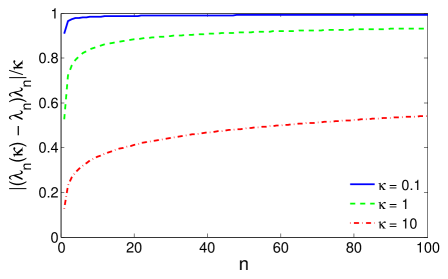
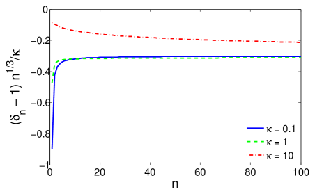
Figure 1 illustrates Proposition 6.2.
Solving Eq. (6.17) numerically, we find the first 100 zeros
with . According to
Proposition 6.2, these zeros are within distance
from the zeros which are given explicitly through the zeros . Moreover,
the second order term in (6.20) that was computed
in [22], suggests that the rescaled distance
(6.25)
behaves as
(6.26)
with a nonzero constant . Figure 1(top) shows that
the distance remains below for three values of
: , , and . The expected asymptotic behavior given in
(6.26) is confirmed by Figure
1(bottom), from which the constant is estimated to
be around .
Figure 1:
Illustration of Proposition 6.2 by the numerical
computation of the first 100 zeros of
(6.17). At the top, the rescaled distance
from (6.25) between and . At the bottom, the asymptotic behavior of this
distance.
Remark 6.5
The local inversion theorem with control with respect to permits
to have the asymptotic behavior of the uniformly
for small:
(6.27)
An improvment of (6.27) (as formulated by
(6.26)) results from a good estimate on .
Observing that in the ball
, we obtain
(6.28)
If one asks for finer estimates, one should compute and
estimate , and so on.
It would also be interesting to analyze the case . See [22] for a preliminary non rigorous analysis. The
limiting problem in this case is the realization of the complex Airy
operator on the line which has empty spectrum.
In the remaining part of this section, we describe the distribution
kernel of the projector associated with .
Proposition 6.6
There exists such that, for any and any , the rank of is
equal to one. Moreover, if is an eigenfunction, then
(6.29)
Proof
To write the projector associated with an eigenvalue
we integrate the resolvent along a small contour
around .
(6.30)
If we consider the associated kernels, we get, using
(6.14) and the fact that is
holomorphic in :
(6.31)
The projector is given by the following expression (with ) for
(6.32)
and for
(6.33)
Here we recall that we have established that for small
enough . It remains to show that the rank of
is one and we will get at the same time an expression for
the eigenfunction. It is clear that the rank of is at
most two and that every function in the range of has the
form , where . It remains to
establish the existence of a relation between and . This
is a consequence of . If ,
the functions in the range have the form
Inequality (6.29) results from an abstract lemma in [6]
once we have proved that the rank of the projector is one. We have
indeed
(6.34)
More generally, the proof of the proposition can be formulated in this
way:
Proposition 6.7
If and , then the
associated projector has rank (no Jordan block).
The condition of being small in Proposition 6.6
is only used for proving the property . For the
case of the Dirichlet or Neumann realization of the complex Airy
operator in , we refer to Section 3. The
nonemptiness was obtained directly by using the properties of the Airy
function. Note that our numerical solutions did not reveal projectors
of rank higher than . We conjecture that the rank of these
projectors is for any but can only
prove the weaker
Proposition 6.8
For any , there is at most a finite number of
eigenvalues with nontrivial Jordan blocks.
Proof
We start from
and get by derivation
(6.35)
What we have to prove is that is different from for
a large solution of . We know already
that . We note that . Hence is not
a pole for . More generally is real and strictly
positive on the real axis. Hence on the real
axis.
We can assume that (the other case can be treated
similarly). Using the equation satisfied by the Airy function, we get
Using the last equality and the asymptotics (A.5), (A.6) for
and , we get as satisfying the
previous condition
which cannot be true for large. This achieves the proof of
the proposition.
7 Resolvent estimates as
The resolvent estimates have been already proved in Section 5
and were used in the analysis of the decay of the associated
semigroup. We propose here another approach which leads to more
precise results. We keep in mind (6.14) and the
discussion in Section 5.
For ,
we have
Hence the Hilbert-Schmidt norm of the resolvent does not depend on the imaginary part of
.
As a consequence, to recover Lemma 5.2 by this approach, it
only remains to check the following lemma
Lemma 7.1
For any , there exist and such that
(7.1)
The proof is included in the proof of the following improvement which
is the main result of this section and is confirmed by the numerical
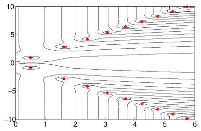
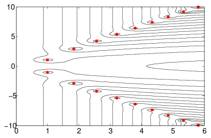
computations. One indeed observes that the lines of the
pseudospectrum are asymptotically vertical as when , see Figure 2.
Figure 2:
Numerically computed pseudospectrum in the complex plane of the
complex Airy operator with Neumann boundary conditions (top) and with
the transmission boundary condition at the origin with
(bottom). The red points show the poles found
by solving numerically Eq. (6.17) that corresponds to the
original problem on . The presented picture corresponds to a zoom
(eliminating numerical artefacts) in a computation done for a large
interval with Dirichlet boundary conditions at . The
pseudospectrum was computed with by projecting the complex
Airy operator onto the orthogonal basis of eigenfunctions of the
corresponding Laplace operator and then diagonalizing the obtained
truncated matrix representation (see Appendix E for
details). We only keep a few lines of pseudospectra for the clarity
of the picture. As predicted by the theory, the vertical lines are
related to the pseudospectrum of the free complex Airy operator on the
line.
Proposition 7.2
For any ,
Moreover, this convergence is uniform for in a compact
set.
Proof
We have
and
Then according to (A.6), one can easily check that the term
decays exponentially as
and grows exponentially as
. On the other hand, the term
decays exponentially as
.
More precisely, we have
(7.2)
As a consequence, the function , which was defined in
(6.10) by
has the following asymptotic behavior as :
(7.3)
We treat the case (the other case can be deduced by
considering the complex conjugate).
Coming back to the two formulas
giving in (6.15) and (6.16) and
starting with the first one, we have to analyze the norm over
of
This norm is given by
Hence we have to estimate .
We observe that
This is rather simple for because and have the
same sign. We can use the asymptotics (A.5)
in order to get
(7.4)
Here we have used that, for ,
We use the control of
given in (7.2) and (7.3) to finally obtain
(7.5)
By the notation , we mean that there exists a constant
such that
and having in mind (7.4), we have only to bound
We can no more use the asymptotic for the Airy function as
is small. We have indeed
We rewrite the integral as the sum
The integral in the middle of the r.h.s. is bounded. The first one is
also bounded according to the behavior of the Airy function. So the
dominant term is the third one
Combining with (7.4), the -norm of the second term decays
as :
(7.6)
This achieves the proof of the proposition, the uniformity for
in a compact being controlled at each step of the proof.
8 Proof of the completeness
We have already recalled or established in Section 3
(Propositions 3.5, 3.9, and 3.12) the results
for the Dirichlet, Neumann or Robin realization of the complex Airy
operator in . The aim of this section is to establish
the same result in the case with transmission. The new difficulty is
that the operator is no more sectorial.
8.1 Reduction to the case
We first reduce the analysis to the case by comparison of
the two kernels. We have indeed
(8.1)
where denotes the kernel of the
resolvent for the transmission problem associated to
and .
We will also use the alternative equivalent
relation:
(8.2)
Remark 8.1
This formula gives another way for proving that the operator with
kernel is in a suitable
Schatten class (see Proposition 4.3). It is indeed enough to
have the result for , that is to treat the Neumann case on
the half line.
Another application of this formula is
Proposition 8.2
There exists such that for all ,
(8.3)
Proof Proposition 8.2 is a consequence of Proposition
3.10, and Formula (8.1).
Remark 8.3
Similar estimates are obtained in the case without boundary (typically
for a model like the Davies operator ) by
Dencker-Sjöstrand-Zworski [13] or more recently by Sjöstrand
[34].
Hence we are reduced to the case which can be decoupled
(see Remark 6.1) in two Neumann problems on and
.
Using (8.2) and the estimates established for (which depends only on ) (see (3.7) or (3.5)), we have
Proposition 8.6
For all , there exist a constant and such
that, for all , for all real , one has
(8.11)
This immediately implies
Proposition 8.7
For any , in , we have
(8.12)
where denotes the scalar product
in the Hilbert space .
We now adapt the proof of the completeness from [2].
If we denote by the closed space generated by the generalized
eigenfunctions of , the proof of [2] in the
presentation of [27] consists in introducing
where
(8.13)
As a consequence of the assumption on , one observes that
is an entire function and the problem is to show that
is identically . The completeness is obtained if we prove this for
any and satisfying the condition (8.13).
Outside the numerical range of , i.e. in the negative
half-plane, it is immediate to see that tends to zero as
. If we show that for some in the whole complex plane, we will
get by Liouville’s theorem that is a polynomial and, with the
control in the left half-plane, we should get that is identically
.
Hence it remains to control in a neighborhood of
the positive half-plane .
As in [2], we apply Phragmen-Lindelöf principle (See Appendix
D). The natural idea (suggested by the numerical picture) is
to control the resolvent on the positive real axis. We first recall
some additional material present in Chapter 16 in
[2].
Theorem 8.8
Let be an entire complex valued function of finite
order . Then for any there exists a sequence such that
For this theorem (Theorem 6.2 in [2]), S. Agmon refers to the
book of Titchmarsh [37] (p. 273).
This theorem is used for proving an inequality of the type with
in the Hilbert-Schmidt case. We avoid an abstract lemma
[2] (Lemma 16.3) but follow the scheme of its proof for
controlling directly the Hilbert-Schmidt norm of the resolvent along
an increasing sequence of circles.
Proposition 8.9
For , there exists a sequence
such that
Proof.
We start from
(8.14)
We apply Theorem 8.8 with . It is proven in Lemma 8.4 that is of type
. Hence we get for (arbitrary small) the
existence of a sequence such that
In view of (8.14), it remains to control the Hilbert-Schmidt norm of
Hence the remaining needed estimates only concern the case
. The estimate on the Hilbert-Schmidt norm of is recalled in (3.7). It remains to get an estimate
for the entire function .
Because , this can be reduced to a question for the
Neumann problem on the half-line for the complex Airy operator . For and , is given by the following expression
(8.15)
We only need the estimate for in a sector containing
. This is done in [27] but we
will give a direct proof below. In the other region, we can first
control the resolvent in and then use the resolvent
identity
This shows that in order to control the Hilbert-Schmidt norm of
for any , it is enough to
control the Hilbert-Schmidt norm of
for some , as well as the norm of
, the latter being easier to
estimate.
More directly the control of the Hilbert-Schmidt norm is reduced to
the existence of a constant such that
In this case, we have to control the resolvent in a neighborhood of
the sector , which corresponds to
the numerical range of the operator.
As , the dominant term in the argument of the Airy
function is .
As expected we arrive in a zone of the complex plane where the Airy
function is exponentially decreasing. It remains to estimate for
which we enter in this zone. We claim that there exists
such that if and , then
In the remaining zone, we obtain easily an upper bound of the integral
by .
We will then use the Phragmen-Lindelöf principle (Theorem
D.1). For this purpose, it remains to control the resolvent on
the positive real line. It is enough to prove the theorem for
and . In other words, it is enough to
consider (resp. ) associated with (resp. ).
Let us treat the case of and use Formula (8.2) and
Proposition 8.7:
(8.16)
This estimate is true on the positive real axis. It remains to
control the term . Along this positive real axis, we have by Proposition
3.10 the decay of . Using Phragmen-Lindelöf principle
completes the proof.
Note that for , we have to use the symmetric (with
respect to the real axis) curve in .
In summary, we have obtained the following proposition
Proposition 8.10
For any , the space generated by the generalized
eigenfunctions of the complex Airy operator with transmission is dense
in .
Appendices
Appendix A Basic properties of the Airy function
In this Appendix, we summarize the basic properties of the Airy
function and its derivative that we used (see
[1] for details).
We recall that the Airy function is the unique solution of
on the line such that tends to as and
This Airy function extends into a holomorphic function in .
The Airy function is positive decreasing on but has an
infinite number of zeros in . We denote by () the decreasing sequence of zeros of . Similarly we
denote by the sequence of zeros of . They have the
following asymptotics (see for example [1]), as ,
(A.1)
and
(A.2)
The functions and (with
) are two independent solutions of the differential
equation
Considering their Wronskian, one gets
(A.3)
Note that these two functions are related to by the identity
(A.4)
The Airy function and its derivative satisfy different asymptotic
expansions depending on their argument:
(i) For ,
(A.5)
(A.6)
(moreover is, for any , uniform when ) .
(ii) For ,
(moreover is for any , uniform in the sector
).
Appendix B Analysis of the resolvent of on the line for (after [31])
On the line , is the closure of the operator
defined on by . A detailed description of its properties can be
found in [25]. In this appendix, we give the asymptotic
control of the resolvent as . We successively discuss the control in and in the Hilbert-Schmidt space . These two spaces are equipped with their
canonical norms.
B.1 Control in .
Here we follow an idea present in the book of Davies [12] and
used in Martinet’s PHD [31] (see also [25]).
Proposition B.1
For all ,
(B.1)
Proof The proof is obtained by considering in
the Fourier space, i.e.
(B.2)
The associated semi-group is
given by
(B.3)
appears as the composition of a multiplication by and a translation by . Computing leads to
(B.4)
It is then easy to get an upper bound for the resolvent. For , we have
(B.5)
(B.6)
(B.7)
The right hand side can be estimated by using the Laplace integral
method. Setting , we have
(B.8)
We observe that admits a global
non-degenerate maximum on at with and . The Laplace integral
method gives the following equivalent as :
(B.9)
This completes the proof of the proposition. We note that this upper
bound is not optimal in comparison with Bordeaux-Montrieux’s formula
(3.5).
B.2 Control in Hilbert-Schmidt norm
In this part, we give a proof of Proposition 3.2. As in
the previous subsection, we use the Fourier representation and analyze
. Note that
(B.10)
We have then an explicit description of the resolvent by
Hence, we have to compute
After the change of variable
,
we get
With
(B.11)
we can write
(B.12)
where
(B.13)
with
(B.14)
can now be split in three terms
(B.15)
with
We observe now that by the change of variable ,
we get
and that
with
Hence, it remains to estimate, as , the integrals and
.
Control of
The function is positive on and negative
decreasing on (). It
admits a unique (non degenerate) maximum at with .
Using the trivial estimates
and
we can estimate from above in the following way
Hence we have shown the existence of and such that, for
,
(B.16)
Hence and appear as remainder terms.
Asymptotic of
Here, using the properties of , we get by the standard Laplace
integral method
(B.17)
Hence, putting altogether the estimates, we get, as ,
(B.18)
Coming back to (B.10), (B.11) and (B.12), this
achieves the proof of Proposition 3.2.
Appendix C Analysis of the resolvent for the Dirichlet realization in the half-line.
C.1 Main statement
The aim of this appendix is to give the proof of Proposition
3.6. Although it is not used in our main text, it is
interesting to get the main asymptotic for the Hilbert-Schmidt norm of
the resolvent in Proposition 3.6.
Proposition C.1
As , we have:
(C.1)
C.2 The Hilbert-Schmidt norm of the resolvent for real
The Hilbert-Schmidt norm of the resolvent can be written as
We note indeed that and that we have a control of
the argument which permits to apply (A.5).
Similarly, we obtain
(C.8)
We note indeed that and so that one can then again apply
(A.5). In particular the function grows
super-exponentially as .
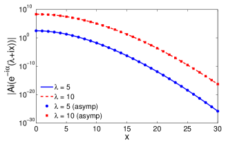
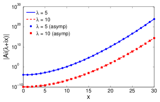
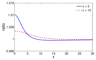
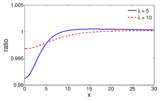
Figure 3 illustrates that, for large ,
both equations (C.6) and (C.8) are
very accurate approximations for and
, respectively.
The control of the next order term (as given in (A.5)) implies
that there exist and , such that, for any , any
and any , one has
(C.9)
(C.10)
and
(C.11)
(C.12)
where the function is explicitly defined in Eq. (C.7).
Basic properties of . Note that
(C.13)
and has the following expansion at the origin
(C.14)
For large , one has
(C.15)
One concludes that the function is monotonously increasing from
to infinity.
There exist and , such that, for any , for , the integral of
can be bounded as
(C.20)
where
(C.21)
Control of .
It remains to control as . Using a change of variables, we get
(C.22)
Hence, introducing
(C.23)
we reduce the analysis to defined for by
(C.24)
with
(C.25)
The following analysis is close to that of the asymptotic behavior of
a Laplace integral.
Asymptotic upper bound of .
Although in the domain of integration in Eq. (C.24), a direct
use of this upper bound will lead to an upper bound by .
Let us start by a heuristic discussion. The maximum of
should be on . For small, we have . This suggests a concentration near , whereas a
contribution for large is of smaller order.
More rigorously, we
write
(C.26)
with, for ,
(C.27)
We now observe that has the form where , so that
(C.28)
Analysis of .
Using the right hand side of inequality (C.28) with
, we show the existence of constants and
, such that,
(C.29)
with
which has now to be estimated for large .
For , we write
with
Using the trivial estimate
we get
(C.30)
We have now to analyze .
The formula giving can be expressed by using
the Dawson function (cf [1], p. 295 and 319)
and its asymptotics as ,
(C.31)
where the function satisfies .
We get indeed
By taking small enough to use the asymptotics of
,
(C.32)
Hence we have shown the existence of constants and
such that if and
(C.33)
Analysis of We start from
and will determine the choice of for a good estimate. Having in
mind the properties of , we can choose large enough in order
to have for some the property that for and
,
(C.34)
This determines our choice of .
Using these inequalities, we rewrite as the sum
with
Using the monotonicity of , we obtain the upper bound
Hence, there exists such that as ,
(C.35)
The last term to control is . Using
(C.34), we get
(C.36)
Hence putting together (C.35) and (C.36) we have,
for this choice of , the existence of and such that
(C.37)
Analysis of .
We recall that
We first observe that
with
Using now
we get
(C.38)
Putting together (C.26), (C.33),
(C.37) and (C.38), we have shown the existence of
and such that if and
(C.39)
Coming back to (C.25) and using (C.18), we
show the existence of and such that if :
Taking , we obtain
Lemma C.3
There exist and such that for
Figure 3:
(Top) Asymptotic behavior of (left)
and (right) for large . (Bottom)
The ratio between these functions and their asymptotics given by
(C.6) and (C.8).
C.5 Lower bound
Once the upper bounds established, the proof of the lower bound is
easy. We start from the simple lower bound (for any )
(C.40)
and consequently
(C.41)
Taking and using the upper bound (C.17),
it remains to find a lower bound for
, which can be worked out in the same way as for the upper bound.
We can use (C.20), (C.29), (C.32) and
(C.42)
This gives the proof of
Lemma C.4
There exist and such that for
Appendix D Phragmen-Lindelöf theorem
The Phragmen-Lindelöf Theorem (see Theorem in [2])
reads
Theorem D.1
(Phragmen-Lindelöf)
Let us assume that there exist two rays
with such that
and a continuous function in
the closed sector delimited by the two rays, holomorphic in the open
sector, satisfying the properties
•
•
There exist an increasing sequence tending to , and
such that
(D.1)
with .
Then we have
for all between the two rays and
.
Appendix E Numerical computation of eigenvalues
In order to compute numerically the eigenvalues of the realization of the complex Airy operator on the real line with a
transmission condition, we impose auxiliary Dirichlet boundary
conditions at , i.e., we search for eigenpairs
of the following problem:
(E.1)
with a positive parameter .
Since the interval is bounded, the spectrum of the above
differential operator is discrete. To compute its eigenvalues, one
can either discretize the second derivative, or represent this
operator in an appropriate basis in the form of an
infinite-dimensional matrix. Following [20], we choose
the second option and use the basis formed by the eigenfunctions of
the Laplace operator with the above boundary
conditions. Once the matrix representation is found, it can be
truncated to compute the eigenvalues numerically. Finally, one
considers the limit to remove the auxiliary boundary
conditions at .
There are two sets of Laplacian eigenfunctions in this domain:
(i) symmetric eigenfunctions
(E.2)
enumerated by the index .
(ii) antisymmetric eigenfunctions
(E.3)
with , where
() satisfy the equation
(E.4)
while the normalization constant is
(E.5)
The solutions of Eq. (E.4) lie in the intervals
, with .
In what follows, we use the double index to distinguish
symmetric and antisymmetric eigenfunctions and to enumerate
eigenvalues, eigenfunctions, as well as the elements of governing
matrices and vectors. We introduce two (infinite-dimensional)
matrices and to represent the Laplace operator and the
position operator in the Laplacian eigenbasis:
(E.6)
and
(E.7)
The symmetry of eigenfunctions implies , while
(E.8)
The infinite-dimensional matrix represents the
complex Airy operator on the interval in the Laplacian
eigenbasis. As a consequence, the eigenvalues and eigenfunctions can
be numerically obtained by truncating and diagonalizing this matrix.
The obtained eigenvalues are ordered according to their increasing
real part:
Table 1 illustrates the rapid convergence of these
eigenvalues to the eigenvalues of the complex Airy operator on the whole line with transmission, as increases. The
same matrix representation was used for plotting the pseudospectrum of
(Fig. 2).
4
0.5161 - 0.8918i
1.2938 - 2.1938i
3.7675 - 1.9790i
6
0.5094 - 0.8823i
1.1755 - 3.9759i
1.6066 - 2.7134i
8
0.5094 - 0.8823i
1.1691 - 5.9752i
1.6233 - 2.8122i
10
0.5094 - 0.8823i
1.1691 - 7.9751i
1.6241 - 2.8130i
0.5094 - 0.8823i
1.6241 - 2.8130i
4
1.0516 - 1.0591i
1.3441 - 2.0460i
4.1035 - 1.7639i
6
1.0032 - 1.0364i
1.1725 - 3.9739i
1.7783 - 2.7043i
8
1.0029 - 1.0363i
1.1691 - 5.9751i
1.8364 - 2.8672i
10
1.0029 - 1.0363i
1.1691 - 7.9751i
1.8390 - 2.8685i
1.0029 - 1.0363i
1.8390 - 2.8685i
Table 1:
The convergence of the eigenvalues computed by
diagonalization of the matrix truncated to the size
. Due to the reflection symmetry of the interval, all
eigenvalues appear in complex conjugate pairs: . The last line presents the poles of the resolvent
of the complex Airy operator obtained by solving
numerically the equation (6.17). The intermediate column
shows the eigenvalue coming from the auxiliary
boundary conditions at (as a consequence, it does not
depend on the transmission coefficient ). Since the imaginary
part of these eigenvalues diverges as , they can be
easily identified and discarded.
References
[1] M. Abramowitz and I. A. Stegun.
Handbook of Mathematical Functions.
Dover Publisher, New York, 1965.
[2] S. Agmon.
Elliptic boundary value problems.D. Van Nostrand Company, 1965.
[3]Y. Almog.
The stability of the normal state of superconductors in the presence of electric currents.
Siam J. Math. Anal. 40 (2) (2008).
824-850.
[4] Y. Almog and B. Helffer.
On the spectrum of non-selfadjoint Schrödinger operators with compact resolvent.
Preprint, arXiv:1410.5122. Comm. in PDE 40 (8), 1441-1466 (2015).
[5] Y. Almog and R. Henry.
Spectral analysis of a complex Schrödinger operator in the semiclassical limit.
arXiv:1510.06806.
[6] A. Aslanyan and E.B. Davies.
Spectral instability for some Schrödinger operators.
ArXiv 9810063v1 (1998).
[7] C. Bardos, D. S. Grebenkov, and A. Rozanova-Pierrat.
Short-time heat diffusion in compact domains with discontinuous transmission boundary conditions.
Math. Models Methods Appl. Sci. 26, 59-110 (2016).
[8] K. Beauchard, B. Helffer, R. Henry and L. Robbiano.
Degenerate parabolic operators of Kolmogorov type with a geometric control condition.
ESAIM Control Optim. Calc. Var. 21 (2), 487–512 (2015).
[9] W. Bordeaux-Montrieux.
Estimation de résolvante et construction de
quasimode près du bord du pseudospectre.
arXiv:1301.3102v1.
[10] H. S. Carslaw and J. C. Jaeger.
Conduction of heat in solids.Clarendon Press, Oxford, 1986.
[12] E.B. Davies.
Linear operators and their spectra.
Cambridge Studies in Advanced Mathematics (N 106) p.250 251.
[13] N. Dencker, J. Sjöstrand, and M. Zworski.
Pseudospectra of (pseudo) differential operators.
Comm. Pure Appl. Math. 57, 384-415 (2004).
[14] T. M. de Swiet and P. N. Sen.
Decay of nuclear magnetization by bounded diffusion in a constant field gradient.
J. Chem. Phys. 100, 5597 (1994).
[15]
N. Dunford and J. T. Schwartz. Linear operators. Part 2: Spectral
theory, self adjoint operators in Hilbert space. New York, 1963.
[16] D.E. Edmunds and W.D. Evans.
Spectral theory and differential operators.Oxford University Press, Oxford, 1987.
[17] P. B. Gilkey and K. Kirsten.
Heat Content Asymptotics with Transmittal and Transmission Boundary Conditions.
J. London Math. Soc. 68, 431-443 (2003).
[18] D. S. Grebenkov.
NMR Survey of Reflected Brownian Motion.
Rev. Mod. Phys. 79, 1077 (2007).
[19] D. S. Grebenkov.
Pulsed-gradient spin-echo monitoring of restricted diffusion in multilayered structures.
J. Magn. Reson. 205, 181-195 (2010).
[20] D. S. Grebenkov, D. V. Nguyen, and J.-R. Li.
Exploring diffusion across permeable barriers at high gradients. I. Narrow pulse approximation.
J. Magn. Reson. 248, 153-163 (2014).
[21] D. S. Grebenkov.
Exploring diffusion across permeable barriers at high gradients. II. Localization regime.
J. Magn. Reson. 248, 164-176 (2014).
[22] D. Grebenkov.
Supplementary materials to [21].
[23] D. Grebenkov, B. Helffer.
On spectral properties of the Bloch-Torrey operator in two dimensions.
Work in progress.
[24] B. Helffer.
On pseudo-spectral problems related to a time dependent model in superconductivity with electric current.
Confluentes Math. 3 (2), 237-251 (2011).
[25] B. Helffer.
Spectral theory and its applications.Cambridge University Press, 2013.
[26] B. Helffer and J. Sjöstrand.
From resolvent bounds to semigroup bounds, Appendix of a course by J. Sjöstrand.
Proceedings of the Evian Conference, 2009, arXiv:1001.4171
[27] R. Henry.
Etude de l’opérateur de Airy complexe.
Mémoire de Master 2 (2010).
[28] R. Henry.
Spectral instability for the complex Airy operator and even non self-adjoint anharmonic oscillators.
J. Spectral theory 4: 349–364 (2014).
[29]
R. Henry.
On the semi-classical analysis of Schrödinger operators with purely
imaginary electric potentials in a bounded domain.
To appear in Comm. in PDE (2015).
[30]
T. Kato.
Perturbation Theory for Linear operators.
Springer-Verlag, Berlin New-York, 1966.
[31] J. Martinet.
Sur les propriétés spectrales d’opérateurs
non-autoadjoints
provenant de la mécanique des fluides.
Thèse de doctorat Univ. Paris-Sud, Déc. 2009. Appendix B.
[32] E. G. Novikov, D. van Dusschoten, and H. Van As.
Modeling of Self-Diffusion and Relaxation Time NMR in Multi-Compartment Systems.
J. Magn. Reson. 135, 522 (1998).
[33] J. G. Powles, M. J. D. Mallett, G. Rickayzen, and W. A. B. Evans.
Exact analytic solutions for diffusion impeded by an infinite array of partially permeable barriers.
Proc. R. Soc. London. A 436, 391-403 (1992).
[34] J. Sjöstrand.
Resolvent estimates for non-selfadjoint operators via semigroups.
Around the research of Vladimir Maz’ya. III.
Int. Math. Ser. 13, Springer, New York, 359–384 (2010).
[35] S. D. Stoller, W. Happer, and F. J. Dyson.
Transverse spin relaxation in inhomogeneous magnetic fields,
Phys. Rev. A 44, 7459-7477 (1991).
[36] J. E. Tanner.
Transient diffusion in a system partitioned by permeable barriers. Application to NMR measurements with a pulsed field gradient.
J. Chem. Phys. 69, 1748 (1978).
[37] E.C. Titchmarsh.
The theory of functions.
2-nd edition, Oxford University Press (1939).
[38] H. C. Torrey.
Bloch equations with diffusion terms.
Phys. Rev. 104, 563 (1956).
[39] O. Vallée and M. Soares.
Airy functions and applications to physics.Imperial College Press, London, (2004).