Analytic and Monte Carlo Studies of Jets with Heavy Mesons and Quarkonia

Abstract

We study jets with identified hadrons in which a family of jet-shape variables called angularities are measured, extending the concept of fragmenting jet functions (FJFs) to these observables. FJFs determine the fraction of energy, $z$, carried by an identified hadron in a jet with angularity, $\tau_{a}$. The FJFs are convolutions of fragmentation functions (FFs), evolved to the jet energy scale, with perturbatively calculable matching coefficients. Renormalization group equations are used to provide resummed calculations with next-to-leading logarithm prime (NLL’) accuracy. We apply this formalism to two-jet events in $e^{+}e^{-}$ collisions with $B$ mesons in the jets, and three-jet events in which a $J/\psi$ is produced in the gluon jet. In the case of $B$ mesons, we use a phenomenological FF extracted from $e^{+}e^{-}$ collisions at the $Z^{0}$ pole evaluated at the scale $\mu=m_{b}$. For events with $J/\psi$, the FF can be evaluated in terms of Non-Relativistic QCD (NRQCD) matrix elements at the scale $\mu=2m_{c}$. The $z$ and $\tau_{a}$ distributions from our NLL’ calculations are compared with predictions from monte carlo event generators. While we find consistency between the predictions for $B$ mesons and the $J/\psi$ distributions in $\tau_{a}$, we find the $z$ distributions for $J/\psi$ differ significantly. We describe an attempt to merge PYTHIA showers with NRQCD FFs that gives good agreement with NLL’ calculations of the $z$ distributions.

1 Introduction

The study of jets and heavy flavor continues to play an important role at the Large Hadron Collider (LHC) and many other high energy and nuclear experiments. Such studies are essential for testing our understanding of Quantum Chromodynamics (QCD) and for calculating backgrounds in searches for new physics. In this paper we calculate cross sections for $e^{+}e^{-}$ to jets, where one of the jets contains a hadron with either open or hidden heavy flavor. In particular, we will derive factorization theorems and perform analytical Next-to-Leading-Log prime (NLL’) resummation for these cross sections using renormalization group (RG) techniques. We will also compare our results with monte carlo simulations of the same cross sections.

Recently, there has been considerable interest in cross sections of this type Procura:2009vm ; Liu:2010ng ; Jain:2011xz ; Jain:2011iu ; Procura:2011aq ; Jain:2012uq ; Bauer:2013bza ; Baumgart:2014upa ; Kaufmann:2015hma ; Chien:2015ctp . Ref. Procura:2009vm demonstrated that the cross section for producing a jet with an identified hadron can be determined using a distribution function called the fragmenting jet function (FJF). FJFs are in turn related to the more commonly studied fragmentation functions (FFs) by a matching calculation at the jet energy scale. This implies that cross sections for jets with an identified hadron provide a new arena to measure FFs, which are more commonly extracted from the semi-inclusive cross section $e^{+}e^{-}\to H+X$. Especially important is that this provides an opportunity to extract gluon FFs Kaufmann:2015hma ; Chien:2015ctp , since quark FFs are more readily studied in $e^{+}e^{-}\to H+X$. In addition, it was recently shown in Ref. Baumgart:2014upa that since the FFs for quarkonia production can be calculated in the Non-Relativistic Quantum Chromodynamics (NRQCD) factorization formalism Bodwin:1994jh , FJFs can be used to make novel tests of quarkonium production theory.

The FJF was first introduced in Ref. Procura:2009vm whose main results can be summarized as follows:

• A factorization theorem for a jet with an identified hadron, $H$, is obtained from the factorization theorem for a jet cross section by the replacement

  $$J_{i}(s,\mu)\to\frac{1}{2(2\pi)^{3}}{\cal G}^{H}_{i}(s,z,\mu)dz,$$ (1)

  where $J_{i}(s,\mu)$ is the jet function for a jet with invariant mass $s$ initiated by parton $i$, and the renormalization scale is $\mu$. The FJF, denoted ${\cal G}^{H}_{i}(s,z,\mu)$, additionally depends on the fraction $z$ of the jet energy that is carried by the identified hadron. These functions implicitly depend on the jet clustering algorithm and cone size $R$ used to define the jets. It is also possible to define jet functions and FJFs that depend on the total energy of the jet rather than the invariant mass Procura:2011aq .

• The FJFs, ${\cal G}^{H}_{i}(s,z,\mu)$, are related to the well-known FFs, $D^{H}_{i}(z,\mu)$, by the formulae

  $${\cal G}^{H}_{i}(s,z,\mu)=\sum_{j}\int_{z}^{1}\frac{dz^{\prime}}{z^{\prime}}{\cal J}_{ij}(s,z^{\prime},\mu)D^{H}_{j}(z/z^{\prime},\mu)+{\cal O}\left(\Lambda^{2}_{\rm QCD}/s\right)\,,$$ (2)

  where the coefficients ${\cal J}_{ij}(s,z,\mu)$ are perturbatively calculable matching coefficients whose large logs are minimized at the jet scale, $s$, and are calculated to NLO in Ref. Jain:2011xz . For heavy quarks the ${\cal J}_{ij}(s,z,\mu)$ have been calculated to $O(\alpha_{s}^{2})$ in Ref. Bauer:2013bza .

• These matching coefficients obey the sum rule

  $$J_{i}(s,\mu)=\frac{1}{2(2\pi)^{3}}\sum_{j}\int_{0}^{1}dzz{\cal J}_{ij}(s,z,\mu)\,.$$ (3)

The properties of FJFs were further studied in Refs. Liu:2010ng ; Jain:2011xz ; Jain:2011iu ; Procura:2011aq ; Jain:2012uq . These papers focused on the FJFs for light hadrons such as pions. FJFs for particles with a single heavy quark were studied in Ref. Bauer:2013bza and FJFs for quarkonia were calculated in Ref. Baumgart:2014upa .

One important goal of this work is to generalize FJFs to jets in which the angularity is measured. The angularity, denoted $\tau_{a}$, is defined as Berger:2003iw

$$\tau_{a}=\frac{1}{\omega}\sum_{i}(p_{i}^{+})^{1-a/2}(p_{i}^{-})^{a/2}\,,$$ (4)

where the sum is over all the particles in the jet, and $\omega=\sum_{i}p_{i}^{-}$ is the large light-like momentum of the jet. The angularity should be viewed as a generalization of the invariant mass squared of the jet since $s=\omega^{2}\tau_{0}$. We calculate the matching coefficients appropriate for jets in which the angularity has been measured, denoted ${\cal J}_{ij}(\tau_{a},z,\mu)$, and verify the $s\to\tau_{a}$ generalization of the sum rules in Eq. (3) in Appendix B of this paper. The other goal of this work is to study the $z$ and $\tau_{a}$ dependence of the cross section for jets with identified heavy hadrons in $e^{+}e^{-}$ collisions and compare our analytical results to monte carlo simulations. We will do this for two-jet events in which $e^{+}e^{-}\to b\bar{b}$ is followed by fragmentation to $B$ mesons. We will also study three-jet events with $e^{+}e^{-}\to b\bar{b}g$ followed by the gluon fragmenting to a jet with a $J/\psi$. At the LHC we expect high energy gluons fragmenting to a jet with $J/\psi$ to be an important production mechanism of $J/\psi$ at high $p_{T}$ and Ref. Baumgart:2014upa showed this process is sensitive to the mechanisms underlying quarkonium production. The study in this paper will allow comparison of analytic calculations with monte carlo simulations of gluons fragmenting to $J/\psi$ in jets. In order for this cross section to be physically observable one would either include quarks and antiquarks fragmenting to jets with $J/\psi$ or one would have to ensure experimentally that the $J/\psi$ came from the gluon jet in the three-jet event, which could be possible if the other jets are $b$-tagged.

In Section 2, we discuss the basics of FJFs for events containing jets where the angularity of the one of the jets is probed. We review various properties of FJFs and their relationship with the more commonly studied FFs. We also present our results for the matching coefficients $\mathcal{J}_{ij}(\tau_{a},z,\mu)$ for jets with measured angularities. Further details of that calculation can be found in Appendix B. In Section 3, we present our results for the NLL’ cross section for $e^{+}e^{-}\to 2$ jets where one of the jets contains a $B$ meson and the angularity of that jet is measured. We find reasonable agreement in both $z$ and $\tau_{a}$ distributions between our analytic calculations and monte carlo simulations performed using Madgraph Alwall:2014hca $+$ PYTHIA Sjostrand:2006za ; Sjostrand:2014zea and Madgraph $+$ HERWIG Bahr:2008pv . In Section 4, we show similar comparisons of analytic versus monte carlo calculations for the cross section for $e^{+}e^{-}\to 3$ jets where one of the jets contains a $J/\psi$ created via gluon fragmentation. In this case the $\tau_{a}$ distributions for the jet are in good agreement, but the monte carlo predictions for the $z$ distributions are inconsistent. We believe that this is due to PYTHIA’s modeling of radiation from color-octet states that produces a harder $z$ distribution than the analytic calculations. In an effort to improve the consistency between NLL’ and monte carlo calculations, we turn off hadronization in PYTHIA and then convolve the distribution of momenta of the gluons within a jet with the NRQCD color-octet FF at the scale $2m_{c}$. This ad-hoc procedure brings monte carlo calculations into much better agreement with analytic NLL’ calculations. This suggests that if NRQCD fragmentation could be properly implemented in PYTHIA, consistency with NLL’ calculations would be obtained, though more work needs to be done on this problem. In Section 5 we give our conclusions. Appendix A summarizes the renormalization group evolution (RGE) needed for NLL’ calculations and also gives the profile functions that are used when computing the scale variation in the NLL’ calculations. Appendix B describes the calculation of the matching coefficients and checks that they satisfy the required sum rules that relate them to the jet function.

2 Fragmenting Jet Functions with Angularities

In this section we extend the calculation of Ref. Jain:2011xz to FJFs with measured angularities. We will follow the terminology of Ref. Ellis:2010rwa , in which a jet whose angularity is measured is referred to as a “measured” jet, while a jet for whom only the total energy is measured but the angularity is not is called an “unmeasured” jet. Here we consider the case of two particles as this is the most that will appear in a one-loop calculation. In Ref. Jain:2011xz the measurement operator in the definition of FJFs forces the mass squared of the jet to be $s$. The measurement operator takes the form

$$\delta(\omega(k^{+}-l^{+}-p^{+}))=\delta(s-\omega(l^{+}+p^{+})),$$ (5)

where $k^{\mu}$ is the parent parton’s momentum and $l^{\mu}$ and $p^{\mu}$ are the momenta of the partons carrying large lightcone components $l^{-}=(1-z)k^{-}$ and $p^{-}=zk^{-}$ of the parent’s momentum, respectively. The operator definition of the FJF with measured angularities is given by

$${\cal{G}}_{i}^{h}(\tau_{a},z,\mu)=\int\frac{dk^{+}dp_{h}^{+}}{2\pi}\int d^{4}y \;e^{-ik^{+}y^{-}/2}$$ (6)

$$\times\sum_{X}\frac{1}{4N_{C}}\mathrm{tr}\Big{[}\frac{n\!\!\!/}{2}\langle 0|\chi_{n,\omega}(y)\delta(\tau_{a}-\hat{\tau}_{a})|Xh\rangle\langle Xh|\bar{\chi}_{n,\omega}(0)|0\rangle\Big{]}$$

where at $\mathcal{O}(\alpha_{s})$ the operator $\hat{\tau}_{a}$ takes the form (cf. Eq. (4))

$$\delta(\tau_{a}-((l^{+})^{1-a/2}(l^{-})^{a/2}-(p^{+})^{1-a/2}(p^{-})^{a/2})/\omega)\,.$$ (7)

Other than replacing Eq. (5) with Eq. (7), the integrals of all diagrams are the same as in Ref. Jain:2011xz . However, rather than using the $\delta$-regulator and a gluon mass, we will use pure dimensional regularization to regulate all divergences. In this limit, it is possible to show that the one-loop evaluation of the FF yields

$$D_{i\rightarrow j}(z)=\delta_{ij}\delta(1-z)+T_{ij}\frac{\alpha_{s}}{2\pi}P_{ij}(z)\left(\frac{1}{\epsilon_{UV}}-\frac{1}{\epsilon_{IR}}\right)\,,$$ (8)

where $T_{ij}$ are the color structures, $T_{qq}=C_{F},\;T_{gg}=C_{A},\;T_{qg}=C_{F},\;T_{gq}=T_{R}$. Additionally, we have verified that the same $1/\epsilon_{IR}$ poles appear in the calculation of FJFs and appropriately cancel in the matching between the FJFs and FFs for all values of $a<1$. This justifies the formula

$${\cal{G}}_{i}^{h}(\tau_{a},z,\mu)=\sum_{j}\int_{z}^{1}\frac{dx}{x}\;{\cal{J}}_{ij}(\tau_{a},x,\mu)D_{j\rightarrow h}\left(\frac{z}{x},\mu\right),$$ (9)

which is the analog of Eq. (1) for FJFs that depend on the angularities.

Since the matching coefficients ${\cal{J}}_{ij}(\tau_{a},z,\mu)$ are free of IR divergences, we can simplify the matching calculation by using pure dimensional regularization, setting all scaleless integrals to zero and interpreting all $1/\epsilon$ poles as UV. A detailed calculation of the renormalized finite terms of ${\cal{J}}_{ij}(\tau_{a},z,\mu)$ can be found in Appendix B, the results of which are shown below. We parametrize the matching coefficients ${\cal{J}}_{ij}(\tau_{a},z,\mu)$ as

$$\begin{split}\frac{{\cal{J}}_{ij}(\tau_{a},z,\mu)}{2(2\pi)^{3}}&=\delta_{ij}\delta(1-z)\delta(\tau_{a})\\ &+T_{ij}\frac{\alpha_{s}}{2\pi}\Big{[}c_{0}^{ij}(z,\mu)\delta(\tau_{a})+c_{1}^{ij}(z,\mu)\left(\frac{1}{\tau_{a}}\right)_{+}+c_{2}\delta_{ij}\delta(1-z)\left(\frac{\ln\tau_{a}}{\tau_{a}}\right)_{+}\Big{]}\,,\end{split}$$ (10)

where

$$c_{0}^{ij}(z,\mu) =\frac{1-a/2}{1-a}\delta_{ij}\delta(1-z)\Big{[}\ln^{2}\frac{\mu^{2}}{\omega^{2}}-\frac{\pi^{2}}{6}\Big{]}+c^{ij}(z)$$

$$\quad-\bar{P}_{ji}\Bigg{[}\ln\frac{\mu^{2}}{\omega^{2}}+\frac{1}{1-a/2}\ln\left(1+\left(\frac{1-z}{z}\right)^{1-a}\right)+(\delta_{ij}-1)\frac{1-a}{1-a/2}\ln(1-z)\Bigg{]}\,,$$

$$c_{1}^{ij}(z,\mu) =-\frac{2}{1-a}\delta_{ij}\delta(1-z)\ln\frac{\mu^{2}}{\omega^{2}}+\frac{1-a}{1-a/2}\bar{P}_{ij}\,,$$

$$c_{2} =\frac{2}{(1-a)(1-a/2)}\,,$$ (11)

with

$$c^{qq}(z) =1-z+\frac{1-a}{1-a/2}(1+z^{2})\left(\frac{\ln(1-z)}{1-z}\right)_{+}\,,$$

$$c^{gg}(z) =\frac{1-a}{1-a/2}\frac{2(1-z+z^{2})^{2}}{z}\left(\frac{\ln(1-z)}{1-z}\right)_{+}\,,$$

$$c^{qg}(z) =z\,,$$

$$c^{gq}(z) =2z(1-z)\,,$$ (12)

and where the $\bar{P}_{ij}$ are the splitting functions of Ref. Jain:2011xz except for the case $i=j=q$,

$$\begin{split}&\bar{P}_{qq}=P_{qq}-\frac{3}{2}\delta(1-z)=\frac{1+z^{2}}{(1-z)_{+}}\,,\\ &\bar{P}_{gg}=P_{gg}=2\frac{(1-x+x^{2})^{2}}{x(1-x)_{+}}\,,\\ &\bar{P}_{qg}=P_{qg}=x^{2}+(1-x)^{2}\,,\\ &\bar{P}_{gq}=P_{gq}=\frac{1+(1-x)^{2}}{x}\,.\end{split}$$ (13)

Notice that our results for the matching coefficients ${\cal{J}}_{ij}(\tau_{a},z,\mu)$ are independent of the jet algorithm and the jet size parameter $R$. To include modifications of the ${\cal J}_{ij}(\tau_{a},z,\mu)$ that come from these effects, one would have to multiply the measurement operator in Eq. (7) by an additional $\Theta$-function that imposes the phase space constraints required by the jet algorithm. However, for jets with measured angularities, it was shown in Ref. Ellis:2010rwa that jet-algorithm dependent terms for cone and $k_{T}$-type algorithms are suppressed by powers of $\tau_{a}/R^{2}$. Inuitively, this is because as $\tau_{a}\to 0$ all the particles in the jet lie along the jet axis so the result must be insensitive to which algorithm is used and to the value of $R$ in this limit. For the values of $\tau_{a}$ and $R$ considered in this paper, $\tau_{a}/R^{2}$ is negligible and we will drop these corrections.

As a non-trivial check of our results we show in Appendix B that our ${\cal{J}}_{ij}(\tau_{a},z,\mu)$ satisfy the following identities and sum rules,

$$\lim_{a\rightarrow 0}{\cal{J}}_{ij}(\tau_{a},z,\mu)=\omega^{2}{\cal{J}}_{ij}(s,z,\mu)\,,$$ (14)

and

$$J_{i}(\tau_{a},\mu)=\frac{1}{2(2\pi)^{3}}\sum_{j}\int_{0}^{1}dz\;z\;{\cal{J}}_{ij}(\tau_{a},z,\mu)\,,$$ (15)

where ${\cal{J}}_{ij}(s,z,\mu)$ are the matching coefficients for measured jet invariant mass found in Ref. Jain:2011xz and $J_{i}(\tau_{a},\mu)$ are the jet functions for measured jets that can be found in Ref. Ellis:2010rwa .

3 $e^{+}e^{-}\to 2$ Jets with a $B$ Meson

In this section we present an analytic calculation of the cross section for $e^{+}e^{-}$ to two $b$ jets in which the $B$ meson is identified in a measured jet. Following the analysis of Ref. Ellis:2010rwa , the factorization theorem for the cross section for one measured $b$ jet and one unmeasured $\bar{b}$ jet is

$$\frac{1}{\sigma_{0}}\frac{d\sigma}{d\tau_{a}}=H_{2}(\mu)\times S^{\mathrm{unmeas}}(\mu)\times J_{\bar{n}}^{(\bar{b})}(\mu)\times\Big{[}S^{\mathrm{meas}}(\tau_{a},\mu)\otimes J_{n}^{(b)}(\tau_{a},\mu)\Big{]},$$ (16)

where $H_{2}(\mu)$ is the hard function, $S^{\mathrm{unmeas}}(\mu)$ and $S^{\mathrm{meas}}(\tau_{a},\mu)$ are the unmeasured and measured soft functions, $J_{\bar{n}}^{(\bar{b})}(\mu)$ is the unmeasured jet function containing the $\bar{b}$ quark and $J_{n}^{(b)}(\tau_{a},\mu)$ is the measured jet function containing the $b$ quark. These describe the short-distance process, surrounding soft radiation, and radiation collinear to unmeasured and measured jets, respectively. At NLO the $\tau_{a}$-independent functions are given by

$$\begin{split}H_{2}(\mu)&=1-\frac{\alpha_{s}(\mu)C_{F}}{2\pi}\left[8-\frac{7\pi^{2}}{6}+\ln^{2}\frac{\mu^{2}}{\omega^{2}}+3\ln\frac{\mu^{2}}{\omega^{2}}\right]\,,\\ S^{\text{unmeas}}(\mu)&=1+\frac{\alpha_{s}(\mu)C_{F}}{2\pi}\left[\ln^{2}\frac{\mu^{2}}{4\Lambda^{2}}-\ln^{2}\frac{\mu^{2}}{4\Lambda^{2}r^{2}}-\frac{\pi^{2}}{3}\right]\,,\\ J_{\bar{n}}^{(\bar{b})}(\mu)&=1+\frac{\alpha_{s}(\mu)C_{F}}{2\pi}J^{q}_{\rm alg}(\mu),\end{split}$$ (17)

where $\Lambda$ is a veto on out-of-jet energy, $r=\tan{(R/2)}$ and $J^{q}_{\rm alg}(\mu)$ is a function that depends on the algorithm used (and we will use the cone algorithm below) and is given in Eq. (A.18) of Ref. Ellis:2010rwa . We note that unlike measured jets, algorithm dependent contributions to the unmeasured jet are not power suppressed. We also note that, beginning at $\mathcal{O}(\alpha^{2})$, non-global logarithms of the ratio $Q\tau_{a}/(2\Lambda r^{2})$ begin to appear in the cross-section Chien:2015cka . For the values of the parameters we consider, these ratios are such that we can treat these logarithms as $\mathcal{O}(1)$ and thus these would enter as fixed order corrections needed at NNLL’ accuracy, which is beyond the scope of this work.

We suppress the dependence of all these functions on scales other than the renormalization scale $\mu$. Measured functions are convolved according to

$$f(\tau)\otimes g(\tau)=\int d\tau^{\prime}\;f(\tau-\tau^{\prime})g(\tau^{\prime}).$$ (18)

To calculate the differential cross section for a measured jet with an identified $B$ hadron, we apply the analogous replacement rule in Eq. (1) to Eq. (16) and use the expression for the FJF in Eq. (9) to obtain

$$\frac{1}{\sigma_{0}}\frac{d\sigma^{(b)}}{d\tau_{a}dz}=H_{2}(\mu)\times S^{\mathrm{unmeas}}(\mu)\times J_{\bar{n}}^{(\bar{b})}(\mu)\times\sum_{j}\Big{[}\Big{(}S^{\mathrm{meas}}(\tau_{a},\mu)\otimes\frac{{\cal{J}}_{bj}^{(b)}(\tau_{a},z,\mu)}{2(2\pi)^{3}}\Big{)}\bullet D_{j\rightarrow B}(z)\Big{]},$$ (19)

where

$$G(z)\bullet F(z)=F(z)\bullet G(z)\equiv\int_{z}^{1}\frac{dx}{x}F(x)G\Big{(}\frac{z}{x}\Big{)}.$$ (20)

To obtain an NLL’ resummed formula for the cross section, we evaluate each function in the factorization theorem in Eq. (19) at its “characteristic” scale (where potentially large logarithms are minimized) and, using renormalization group techniques, evolve each function to a common scale, $\mu$, which we will choose to be equal to the hard scale. The details of this evolution are discussed in Appendix A.

The convolutions in Eq. (19) must be performed over angularity over $S^{\mathrm{meas}}$, ${\cal{J}}_{ij}$, and factors arising from RG equations. Since such RG factors are distributions ($\delta$ or plus-distributions) in the angularity our final answer is written in terms of distributions that can be computed analytically using Eqs. (43-A.2). Upon performing convolutions and resummation to NLL’ accuracy we find for the cross section

$$d\sigma(\tau_{a},z)\equiv\frac{1}{\sigma_{0}}\frac{d\sigma^{(b)}}{d\tau_{a}dz}=H_{2}(\mu_{H})\times S^{\mathrm{unmeas}}(\mu_{\Lambda})\times J_{\bar{n}}^{(\bar{b})}(\mu_{J_{\bar{n}}})\times$$ (21)

$$\times\sum_{j}\Bigg{\{}\left(\frac{\Theta(\tau_{a})}{\tau_{a}^{1+\Omega}}\right)\Big{[}\delta_{bj}\delta(1-z)\left(1+f_{S}(\tau_{a},\mu_{S^{\mathrm{meas}}})\right)+f_{{\cal{J}}}^{bj}(\tau_{a},z,\mu_{J_{n}})\Big{]}\bullet\frac{D_{j\rightarrow B}(z,\mu_{J_{n}})}{2(2\pi)^{3}}$$

$$\qquad\times\Pi(\mu,\mu_{H},\mu_{\Lambda},\mu_{J_{\bar{n}}},\mu_{J_{n}},\mu_{S^{\mathrm{meas}}})\ \Bigg{\}}_{+},$$

where the ‘$+$’ distribution is defined in Eq. (40) (and acts on all $\tau_{a}$-dependent quantities, including any implicit dependencies arising from the choice of scales $\mu_{F}$) and $\Omega(\mu_{J_{n}},\mu_{S^{\mathrm{meas}}})=\omega_{J_{n}}(\mu,\mu_{J_{n}})+\omega_{S^{\mathrm{meas}}}(\mu_{,}\mu_{S^{\mathrm{meas}}})$, the functions $\omega_{J_{n}}$ and $\omega_{S^{\mathrm{meas}}}$ are given in Appendix A, the function $f_{S}$ is given by Ellis:2010rwa

$$\begin{split}f_{S}(\tau,\mu)&=-\frac{\alpha_{s}(\mu)C_{F}}{\pi}\frac{1}{1-a}\left\{\left[\ln\frac{\mu\tan^{1-a}\frac{R}{2}}{\omega\tau}+H(-1-\Omega)\right]^{2}+\frac{\pi^{2}}{6}-\psi^{(1)}(-\Omega)\right\}\,,\end{split}$$ (22)

and $f_{\cal{J}}^{ij}$ are written in terms of the coefficients $c_{0}^{ij}$, $c_{1}^{ij}$ and $c_{2}$ presented in Eq. (2) as

$$\begin{split}f_{\cal{J}}^{ij}(\tau,z,\mu)&=T_{ij}\frac{\alpha_{s}(\mu)}{2\pi}\Bigg{(}c_{0}^{ij}(z,\mu)+c_{1}^{ij}(z,\mu)\Big{(}\ln\tau-H(-1-\Omega)\Big{)}\\ &+c_{2}\delta_{ij}\delta(1-z)\Big{(}\frac{(\ln\tau-H(-1-\Omega))^{2}+\pi^{2}/6-\psi^{(1)}(-\Omega)}{2}\Big{)}\Bigg{)}.\end{split}$$ (23)

The evolution kernel $\Pi$ is given in terms of $K_{F}(\mu,\mu_{0})$ and $\omega_{F}(\mu,\mu_{0})$ (cf. Appendix A),

$$\Pi(\mu,\mu_{H},\mu_{\Lambda},\mu_{J_{\bar{n}}},\mu_{J_{n}},\mu_{S^{\mathrm{meas}}})=\prod_{F=H,J_{\bar{n}},S^{\mathrm{unmeas}}}\exp(K_{F}(\mu,\mu_{F}))\left(\frac{\mu_{F}}{m_{F}}\right)^{\omega_{F}(\mu,\mu_{F})}$$ (24)

$$\qquad\times\frac{1}{\Gamma(-\Omega(\mu_{J_{n}},\mu_{S^{\mathrm{meas}}}))}\times\prod_{F=J_{n},S^{\mathrm{meas}}}\exp(K_{F}(\mu,\mu_{F})+\gamma_{E}\omega_{F}(\mu,\mu_{F}))\left(\frac{\mu_{F}}{m_{F}}\right)^{j_{F}\omega_{F}(\mu,\mu_{i})}\,,$$

where $\mu_{F},\;m_{F}$ and $j_{F}$ are given in Table 1. Because they involve FFs (cf. Appendix B), the $z$ convolutions must be evaluated numerically. For the fragmentation of the $b$ quark we use a two-parameter power model FF introduced in Ref. Kartvelishvili:1978jh , in which $D_{b\rightarrow B}(z,\;\mu=m_{b}=4.5\;\mathrm{GeV})$ is proportional to $z^{\alpha}(1-z)^{\beta}$. Values for the parameters $\alpha=16.87$ and $\beta=2.628$ with $\chi^{2}_{d.o.f.}=1.495$ were determined using a fit to LEP data in Ref. Kniehl:2008zza for the inclusive process $e^{+}e^{-}\rightarrow B+X$. Errors in these parameters were not quoted in Ref. Kniehl:2008zza , so we cannot quantify errors associated with the extracted FF in our calculation. Additionally, we neglect the contribution from the fragmentation of other partons for our $e^{+}e^{-}$ collider studies as in Ref. Kniehl:2008zza . In proton-proton collisions at the LHC, gluon FJFs must also be included since the dijet channel $gg\rightarrow gg$ gives a significant contribution to the production of jets with heavy flavor Chien:2015ctp . For the evolution of the FF up to the jet scale we solve the DGLAP equation using an inverse Mellin transformation as done in Ref. Baumgart:2014upa .

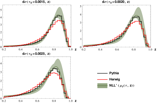
Figure 1: The $z$ distributions for $d\sigma(\tau_{0},z)$ at $\tau_{0}=(1.5,\;2.0,\;2.5)\times 10^{-3}$ for analytic calculations with theoretical uncertainty are shown in green. Monte carlo simulations using Madgraph $+$ PYTHIA and Madgraph $+$ Herwig are shown in black and red, respectively.

Fig. 1 shows the $z$ distributions from $d\sigma(\tau_{0},z)$ for $\tau_{0}=(1.5,\;2.0,\;2.5)\times 10^{-3}$ of our analytic NLL’ calculation (green) and monte-carlo simulations using Madgraph $+$ PYTHIA (black) and Madgraph $+$ HERWIG (red). For each monte carlo and for each NLL’ calculation, the graphs are independently normalized to unit area. For plots with fixed $\tau_{a}$ we use a $z$-bin of $\pm\,0.1$ and for plots with fixed $z$ we use a $\tau_{a}$ bin of size $\pm\,2\times 10^{-4}$. Jets are reconstructed in PYTHIA using the Seedless-Infared-Safe Cone (SISCONE) algorithm in the FastJets package Cacciari:2011ma with $R=0.6$, which will be used throughout this work. We produced simulated dijet events at $E_{cm}=250$ GeV in which each jet has an energy of at least $(E_{cm}-\Lambda)/2$ where $\Lambda=30$ GeV.

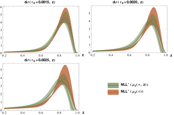
Figure 2: Analytic results for the z distributions of $d\sigma(\tau_{0},z)$ at $\tau_{0}=(1.5,\;2.0,\;2.5)\times 10^{-3}$. The orange curve is calculated with a measured jet scale that does not depend on $z$ whereas the green curve uses a scale that does depend on $z$ (as in Fig. 1).

The central green line corresponds to the NLL’ calculation with the various functions in the factorization theorem evaluated at their characteristic values shown in Table 1, and the green band corresponds to the estimate of theoretical uncertainty obtained by varying the scales of the unmeasured functions by $\pm 50\%$, and using profile functions  Ligeti:2008ac ; Abbate:2010xh ; Hornig:2016ahz to estimate the uncertainty of the measured functions. Profile functions allow us to introduce an angularity dependent scale variation that freezes at the characteristic scale for high values of $\tau_{a}$ where the factorization theorem breaks down and at a fixed scale for small values of $\tau_{a}$ where we reach the non-perturbative regime. This method for estimating theoretical uncertainties is used throughout this work. Additional details on the profile functions we use can be found in Appendix A.

Function $(F)$	$H_{2}$	$J_{\bar{n}}^{\bar{b}}$	$S^{\mathrm{unmeas}}$	${\cal{J}}(\tau,z)$	$S^{\mathrm{meas}}(\tau)$
Scale $(\mu_{F})$	$E_{\mathrm{cm}}$	$\omega_{\bar{n}}r$	$2\Lambda r^{1/2}$	$\omega_{n}\tau^{1/(2-a)}(1-z)^{(1-a)/(2-a)}$	$\omega_{n}\tau/r^{1-a}$
$m_{F}$	$\omega$	$w_{\bar{n}}r$	$2\Lambda r^{1/2}$	$\omega_{n}$	$\omega_{n}/r^{1-a}$
$j_{F}$	$1$	$1$	$1$	$2-a$	$1$

Table 1: Characteristic scales of the different functions in the factorization theorem of Eq. (16).

The orange curves in Fig. 2 show the differential cross section as a function of $z$ for fixed $\tau_{0}$ where $\mu_{J}(\tau)=\mu_{J}(\tau,z=0)=\omega\tau^{1/(2-a)}$ is chosen as the characteristic scale of the measured jet function, and the error band is obtained the same way as for Fig. 1. As in Fig. 1, the green curves show the cross section for a measured jet scale $\mu_{J}(\tau,z)=\omega\tau^{1/(2-a)}(1-z)^{(1-a)/(2-a)}$.

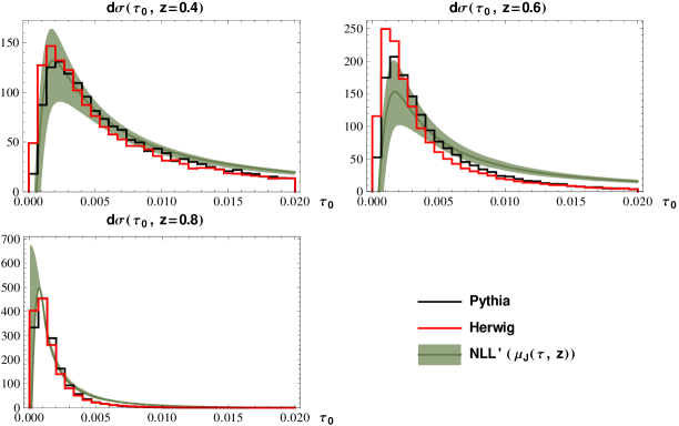
Figure 3: Angularity distributions of $d\sigma(\tau_{a},z)$ for $a=0$ at $z=0.4,\;0.6,\;0.8$. Analytic results are shown as green bands. Monte carlo results are shown as black lines for Madgraph $+$ PYTHIA and red lines for Madgraph $+$ HERWIG.

The reorganization of logarithms of $(1-z)$ shown in Eq. (47) suggests that we can improve the accuracy of our calculations for $z\rightarrow 1$ by choosing the characteristic value of the measured jet scale to be $\mu_{J}(\tau,z)$. This improvement is clearly seen in Fig. 2 which shows the scale variation for the choices $\mu_{J}(\tau)$ and $\mu_{J}(\tau,z)$, the latter choice gives smaller scale variation near the peak in the $z$ distribution.

In Fig. 3 we present the results for the $\tau_{0}$ distributions of the differential cross section $d\sigma(\tau_{a},z)$ for $z=0.4,\;0.6,\;\mathrm{and}\;0.8$. The color and normalization schemes match those in Fig. 1. We see that for higher values of $z$ the distributions of $\tau_{0}$ are shifted towards smaller values. This is expected since the majority of the energy of the jet is carried by the B meson which results in narrower jets. Figs. 1 and 3 show that our results are consistent within the monte carlo uncertainty that is suggested by the difference between PYTHIA and HERWIG predictions. This gives us confidence that the FJF formalism combined with NLL’ resummation can be used to correctly calculate both the substructure and the identified hadron’s energy fraction within a jet.

4 $e^{+}e^{-}\to 3$ Jets with the Gluon Jet Fragmenting to $J/\psi$

We can also use the FJF formalism to calculate the cross section for $e^{+}e^{-}\to 3$ jets with a $J/\psi$. As we expect gluon fragmentation to be the dominant production channel at the LHC, we focus on the case where $J/\psi$ is found within a gluon jet. In addition, we assume that the angularity of this jet is also measured. To obtain a physical observable, one must also include contributions from all jets fragmenting to $J/\psi$, however, we expect the contribution from quark jets to be smaller. It is theoretically possible to isolate the $J/\psi$ coming from gluon jets in experiments by $b$-tagging the other two jets in the event, so we will focus on the process $e^{+}e^{-}\to b\bar{b}g$ followed by gluon fragmentation to $J/\psi$.

The analytic expression for this cross section is

$$\frac{1}{\sigma_{0}}\frac{d\sigma^{(g)}}{d\tau_{a}dz}=H_{3}(\mu_{H})\times S^{\mathrm{unmeas}}(\mu_{\Lambda})\times J_{n_{1}}^{(\bar{b})}(\mu_{J_{n_{1}}})\times J_{n_{2}}^{(b)}(\mu_{J_{n_{2}}})$$

$$\times\sum_{i}\!\Bigg{\{}\!\left(\frac{\Theta(\tau_{a})}{\tau_{a}^{1+\Omega}}\right)\!\Big{[}\delta_{gi}\delta(1-z)(1+f_{S}(\tau_{a},\mu_{S^{\mathrm{meas}}}))+f_{{\cal{J}}}^{gi}(\tau_{a},z,\mu_{J_{n_{3}}})\Big{]}\bullet\frac{D_{i\rightarrow J/\psi}(z,\mu_{J_{n_{3}}})}{2(2\pi)^{3}}$$

$$\qquad\times\Pi(\mu,\mu_{H},\mu_{\Lambda},\mu_{J_{n_{1}}},\mu_{J_{n_{2}}},\mu_{J_{n_{3}}},\mu_{S^{\text{meas}}})\!\Bigg{\}}_{+}\,,$$ (25)

where $\Omega\equiv\Omega(\mu_{J_{n_{3}}},\mu_{S^{\mathrm{meas}}})=\omega_{J_{n}}(\mu,\mu_{J_{n_{3}}})+\omega_{S^{\mathrm{meas}}}(\mu_{,}\mu_{S^{\mathrm{meas}}})$, the $b$-quark initiated jets $J_{n_{1}}^{(b)}$ and $J_{n_{2}}^{(\bar{b})}$ are unmeasured, the expression for $f_{S}$ is the same as Eq. (22) with $C_{F}$ replaced by $C_{A}$, and our expressions for $f_{\cal{J}}^{ij}$ are given in terms of the coefficients $c_{0}^{ij}$, $c_{1}^{ij}$ and $c_{2}$ given in Eq. (2). Here $\sigma_{0}$ is the LO cross section for $e^{+}e^{-}\to b\bar{b}g$. We will focus on the Mercedes Benz configuration in which all three jets have (approximately) the same energy, and consider jets with energies large enough that the mass of $b$-quark can be neglected. Here, $H_{3}(\mu)$ is $1+O(\alpha_{s})$ where the $O(\alpha_{s})$ comes from the NLO virtual corrections to $e^{+}e^{-}\to b\bar{b}g$. We do not include this correction. The primary effect of its omission will be on the normalization of the cross section, which is not important for our discussion of the distributions we show below, and to increase the scale uncertainty associated with varying $\mu_{H}$; however this is not a very important source of uncertainty in our calculations.

While the calculation for $B$ mesons requires a phenomenological FF, the FFs for $J/\psi$ production can be calculated in NRQCD Bodwin:1994jh . Refs. Braaten:1993mp ; Braaten:1993rw ; Braaten:1994vv ; Braaten:1996jt showed that a $J/\psi$ FF can be calculated in terms of analytically calculable functions of $\alpha_{s}(2m_{c})$ and $z$ multiplied by nonperturbative NRQCD long-distance matrix-elements (LDMEs). In $J/\psi$ production, the most important production mechanisms are the color-singlet mechanism, in which the $c\bar{c}$ is produced perturbatively in a ${}^{3}S_{1}^{(1)}$ state, and the color-octet mechanisms, in which the $c\bar{c}$ is produced perturbatively in a ${}^{1}S_{0}^{(8)}$, ${}^{3}S_{1}^{(8)}$, or ${}^{3}P_{J}^{(8)}$ state. Here ${}^{2S+1}L_{J}^{(1,8)}$ refers to the angular momentum and color quantum numbers of the $c\bar{c}$. The numerical values for the corresponding LDMEs are taken to be the central values from the global fits performed in Refs. Butenschoen:2011yh ; Butenschoen:2012qr , and are shown in Table 2.

$\langle\mathcal{O}^{J/\psi}(^{3}S_{1}^{(1)})\rangle$	$\langle\mathcal{O}^{J/\psi}(^{3}S_{1}^{(8)})\rangle$	$\langle\mathcal{O}^{J/\psi}(^{1}S_{0}^{(8)})\rangle$	$\langle\mathcal{O}^{J/\psi}(^{3}P_{J}^{(8)})\rangle/m_{c}^{2}$
1.32 GeV3	2.24 $\times 10^{-3}$ GeV3	$4.97\times 10^{-2}$ GeV3	-7.16 $\times 10^{-3}$ GeV3

Table 2: LDMEs for NRQCD production mechanisms. We use central values taken from global fits in Refs. Butenschoen:2011yh ; Butenschoen:2012qr .

The color-singlet LDME scales as $v^{3}$, where $v$ is the typical relative velocity of the $c\bar{c}$ in the $J/\psi$, while the color-octet LDMEs scale as $v^{7}$ Bodwin:1994jh . This $v^{4}$ suppression is clearly seen in the numerical values of the LDMEs in Table 2. In the calculation of the gluon FF, this $v$ suppression is compensated by powers of $\alpha_{s}$ since the leading color-octet contributions are $O(\alpha_{s}^{2})$ in the ${}^{1}S_{0}^{(8)}$ and ${}^{3}P_{J}^{(8)}$ channels and $O(\alpha_{s})$ in the ${}^{3}S_{1}^{(8)}$ channel, while the color-singlet contribution is $O(\alpha_{s}^{3})$. In this work we focus on the gluon FJF, $\mathcal{G}_{g}^{J/\psi}$, and separately compute each of the four NRQCD contributions to $\mathcal{G}_{g}^{J/\psi}$. To calculate $\mathcal{G}_{g}^{J/\psi}$, we evolve each FF from the scale $\mu=2m_{c}$ to the characteristic scale of the measured jet $\mu_{J_{n_{3}}}(\tau_{a})=\omega\tau_{a}^{1/(2-a)}$ using the DGLAP evolution equations. For most values of $z$ considered in this section, we do not expect that using a $z$ dependent scale will result in significant improvement in the scale variation. In addition, using a $z$ dependent scale in the ${}^{3}P_{J}^{(8)}$ channel yields unphysical results, such as negative values for the FF. After evolution, we perform the convolution $\left[D\bullet f_{\cal{J}}\right](z)$ in $z$ with the matching coefficients derived in Section 3.

Before discussing the comparison of our results with monte carlo, we briefly review how the Madgraph $+$ PYTHIA monte carlo handles color-singlet and color-octet quarkonium production. We produce quarkonia states in Madgraph from the following processes: $e^{+}e^{-}\to b\bar{b}ggc\bar{c}[^{3}S_{1}^{(1)}],\;e^{+}e^{-}\to b\bar{b}gc\bar{c}[^{1}S_{0}^{(8)}]$, and $e^{+}e^{-}\to b\bar{b}c\bar{c}[^{3}S_{1}^{(8)}]$. The quantum numbers ${}^{2S+1}L_{J}^{(1,8)}$ are for the $c\bar{c}$ produced in the event. We only include diagrams in which the virtual photon couples to the $b\bar{b}$ so in all cases the $c\bar{c}$ plus any additional gluons come from the decay of a virtual gluon. We did not simulate production in the ${}^{3}P_{J}^{(8)}$ channel in $e^{+}e^{-}\to b\bar{b}g\to b\bar{b}c\bar{c}g$ because IR divergences in the matrix elements require much longer running times to get the same number of events. We then perform showering and hadronization on these hard processes using PYTHIA. Analysis is done using RIVET Buckley:2010ar . During PYTHIA’s showering phase, color-singlet $J/\psi$ do not radiate gluons. Thus if these $J/\psi$ are produced within a jet, all surrounding radiation is due to the other colored particles in the event Sjostrand:2006za ; Sjostrand:2014zea . We require that after showering there are only three jets in the event, two from the $b$-quarks and one from a gluon that contains the $J/\psi$. We simulate three-jet events at $E_{cm}=250$ GeV in the Mercedes-Benz configuration by requiring the jets each have energies $E_{jet}>(E_{cm}-\Lambda)/3$ with $\Lambda=30$ GeV, analagous to what was done in Sec. 3.

For $c\bar{c}$ produced in a color-octet state PYTHIA allows the color-octet $c\bar{c}$ to emit gluons with a splitting function $2P_{qq}(z)$. Since $P_{qq}(z)$ is peaked at $z=1$, the color-octet $c\bar{c}$ pair typically retains most of its energy after these emissions. This model of the production mechanism is very different than the physical process implied by the NLL’ calculation. In the NLL’ calculation, the FF is calculated at the scale $2m_{c}$, then evolved up to the jet energy scale using Altarelli-Parisi evolution equations. Since this is a gluon FF, the most important splitting kernel in this evolution is $P_{gg}(z)$. We find that the FFs obtained at the jet energy scale are not significantly changed if we use only this evolution kernel and ignore mixing with quarks. Thus the production process implied by the NLL’ calculation is that of a highly energetic gluon produced in the hard process with virtuallity of order the jet energy scale, which then showers by emitting gluons until one of the gluons with virtuality of order $2m_{c}$ hadronizes into the $J/\psi$. Because $P_{gg}(z)$ is peaked at $z=0$ and $z=1$ the resulting $J/\psi$ distribution in $z$ is much softer than the model employed by PYTHIA. PYTHIA does not allow one to change the actual splitting function, only to modify the color-factor. Therefore, in order to get a softer $z$ distribution we changed the coefficient of PYTHIA’s splitting kernel for a gluon radiating off a color-octet $c\bar{c}$ pair from $2P_{qq}$ to $C_{A}P_{qq}=3P_{qq}$. This results in a slighter softer $z$ distribution than default PYTHIA, but is still inconsistent with the NLL’ calculation. This change does not have significant impact on the $\tau_{a}$ distributions. The $\tau_{a}$ distributions are generally in better agreement. The variable $\tau_{a}$ depends on all of the hadrons in the jet and is therefore less sensitive to the behavior of the $J/\psi$, especially when the $J/\psi$ carries a small fraction of the jet energy. In that case, $\tau_{a}$ distributions in the NLL’ calculation look similar for all color-octet mechanisms.

In an attempt to see if PYTHIA can be modified to reproduce the $z$ distributions obtained in our NLL’ calculations, and confirm the physical picture of the NLL’ calculation described above, we generate $e^{+}e^{-}\to b\bar{b}g$ events in Madgraph and allow PYTHIA to shower but not hadronize the events. If we allow the shower to evolve to a scale where the typical invariant mass of a gluon is $2m_{c}$ and then convolve the gluon distribution with the NRQCD FFs at this scale, we expect that the resulting $z$ distributions should mimic our NLL’ calculation. The lower cutoff scale in PYTHIA’s parton shower is set by the parameter TimeShower:pTmin, which is related to the minimal virtuality of the particles in the shower, and whose default value is 0.4 GeV. We change this parameter to 1.6 GeV, which corresponds to a virtuality of $\sim 2m_{c}$, then obtain a $z$ distribution for the gluons by randomly choosing a gluon from the gluon initiated jet. We then numerically convolve this $z$ distribution with the analytic expression for the NRQCD FF. This procedure, which we will refer to as Gluon Fragmentation Improved PYTHIA (GFIP), yields $z$ distributions that are consistent with our NLL’ result, as we will see below. We tested an analogous procedure for two-jet events with $B$ mesons by showering $e^{+}e^{-}\to b\bar{b}$ with PYTHIA with hadronization turned off. We then convolved the resulting $b$ quark distribution with the $b$-quark FF at the scale $2m_{b}$, and found results for $B$ mesons that are consistent with our NLL’ calculations. Note that PYTHIA treats the radiation coming from the octet $c\bar{c}$ pair the same regardless of the angular momentum quantum numbers. In contrast, GFIP like the NLL’ calculation gives different results for all three channels by applying different FFs at the end of the parton shower phase. Also GFIP can be applied to all four NRQCD production mechanisms, since convergence issues for the ${}^{3}P_{J}^{(8)}$ channels are absent.

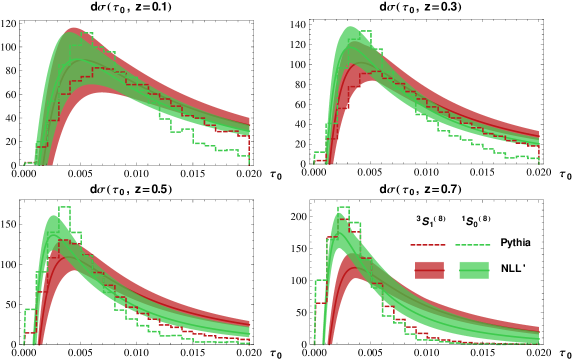
Figure 4: Angularity distributions of $d\sigma(\tau_{a},z)$ for $a=0$ at $z=0,1,\;0.3,\;0.5,\;0.7$. Analytic calculations are shown as red (green) bands for the ${}^{3}S_{1}^{(8)}$ (${}^{1}S_{0}^{(8)}$) production mechanisms. Results from Madgraph $+$ PYTHIA are shown as red (green) dashed lines for the same mechanisms.

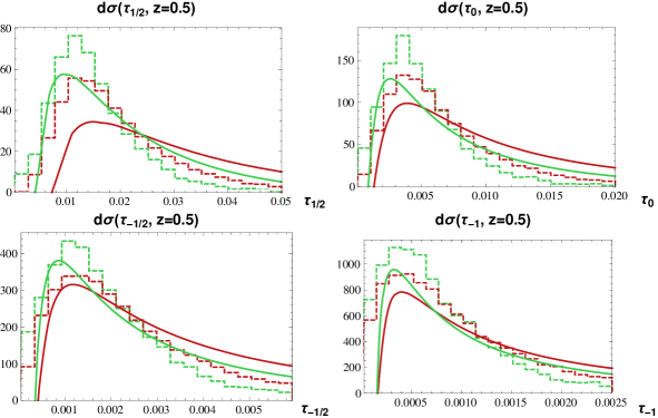
Figure 5: Angularity distributions of $d\sigma(\tau_{a},z)$ for $a=+1/2,\,0,\,-1/2,\,-1$ at $z=0.5$. Analytic calculations are shown as red (green) solid lines for the ${}^{3}S_{1}^{(8)}$ (${}^{1}S_{0}^{(8)}$) production mechanisms. Results from Madgraph $+$ PYTHIA are shown as red (green) dashed lines for the same mechanisms.

Fig. 4 shows our NLL’ calculation and Madgraph $+$ PYTHIA results for the distribution of $\tau_{0}$ for various fixed values of $z$ for the ${}^{3}S_{1}^{(8)}$ (red) and ${}^{1}S_{0}^{(8)}$ (green) channels. We see fairly good agreement between analytic and Monte Carlo results in the peak regions for smaller values of $z$ and notice some qualitative differences in the tail regions, especially for the ${}^{1}S_{0}^{(8)}$ channel. At higher values of $z$ where the number of final state particles is small, differences in the $\tau_{0}$ distributions could be attributed to the increasing influence of Pythia’s unrealistic model of quarkonium production. As $z\to 0$, we also see similar $\tau_{0}$ dependence for the two color-octet channels in our analytic results. This suggests that in the small $z$ region, the jet substructure is independent of the production mechanism. Thus, attempts to use angularity distributions to extract the various LDMEs should focus on the range $0.3<z<0.7$.

In Fig. 5, we show the angularity distributions (without uncertainties) for the ${}^{1}S_{0}^{(8)}$ and ${}^{3}S_{1}^{(8)}$ mechanisms for $a=+1/2,\,0,\,-1/2,\,-1$. These are computed analytically and using monte carlo and we again see reasonable agreement. As $a$ is decreased, we see less discrimination between the two production mechanisms. Thus extraction of LDMEs should ideally be done with larger values of $a$, for $a<1$ where factorization in $\mathrm{SCET}_{I}$ holds, with the caveat that there is a trade-off since the predictability of the analytical results is limited for $a$ too close to $1$ since power corrections grow as $1/(1-a)$ Lee:2006nr .

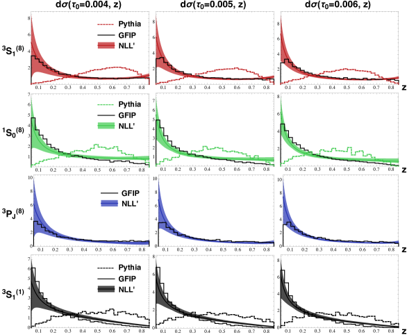
Figure 6: $z$ distributions of $d\sigma(\tau_{a},z)$ for NLL’ analytic calculations (bands), PYTHIA (dashed lines), and GFIP (solid lines) for fixed values of $\tau_{0}=(4,\;5,\;6)\times 10^{-3}$.

In contrast to the angularity distributions, Fig. 6 shows that analytic and monte carlo calculations of the $z$ distributions using Madgraph $+$ PYTHIA yield strikingly different results, with Madgraph+PYTHIA yielding a much harder $z$-distribution. Fig. 6 also shows the $z$ distributions using GFIP. The GFIP modification yields significantly different results for the $z$ distributions that align more closely with NLL’ calculation. While this is far from a proper modification of PYTHIA, it shows us that implementing the missing $g\to J/\psi$ fragmentation yields encouraging similarities to our analytical calculations using the FJF formalism with NRQCD FFs. This also suggests that if monte carlo is modified to properly include NRQCD FFs at the scale $2m_{c}$ it will yield results that are consistent with FJFs combined with NLL’ resummation. Correct monte carlo implementation of the NRQCD FFs is important because the GFIP modification can only be used to calculate the $z$ distribution. There are many other jet shape observables, such as $N$-subjettiness or $\Delta R$ (where $\Delta R$ is the angle between the $J/\psi$ and the jet axis), that should be able to discriminate between NRQCD production mechanisms, and many of these are most easily predicted using monte carlo.

5 Conclusion

The study of hadrons within jets provides new tests of perturbative QCD dynamics. The distribution in $z$ (the fraction of jet energy carried by the identified hadron) can be calculated as a convolution of the well-known fragmentation functions (FFs) for that hadron with perturbative matching coefficients that are calculable at the jet energy scale, which is typically well above $\Lambda_{\rm QCD}$. At hadron colliders this provides a new way to extract FFs and will be especially important for pinning down gluon FFs, which are of subleading importance in $e^{+}e^{-}$ colliders where FFs are usually measured. The production of heavy quarkonia within high energy jets in collider experiments also provides new tests of NRQCD.

In this paper, we studied cross sections for jets with heavy mesons as a function of $z$ and the substructure variable angularity, $\tau_{a}$. We provided for the first time the NLO matching coefficients for jets with measured $\tau_{a}$, and used these along with the known RGE for the hard, jet, and soft functions to obtain NLL’ accuracy calculations of cross sections for jets with heavy mesons. We considered the production of $B$ mesons in two-jet events in $e^{+}e^{-}$ collisions at $E_{\rm cm}=250$ GeV as well as $J/\psi$ production in three-jet events at the same energies. Though not relevant to any experiment, this is useful for comparing NLL’ calculations with monte carlo simulations of fragmenting jets whose energy is comparable to those measured at the LHC. In the simulations of quarkonia production, the underlying hard process was generated using Madgraph and then PYTHIA was used to shower and hadronize the events. In the simulations involving B meson production we also used HERWIG.

For $B$ mesons, we find that the $z$ and $\tau_{a}$ distributions computed using monte carlo and NLL’ are in excellent agreement, giving us confidence in our analytic approach. In the case of $J/\psi$, we considered three-jet events in which the jets all had the same energy and the $J/\psi$ in both simulation and NLL’ calculations was required to come from the gluon jet. This allowed us to study $J/\psi$ production via the fragmentation of high energy gluon initiated jets, which we expect to be an important mechanism at the LHC. Earlier studies of gluon FJFs in Ref. Baumgart:2014upa indicated that the $z$ and $E$ dependence of these jets could discriminate between various NRQCD production mechanisms. The analytic NLL’ studies of this paper are consistent with Ref. Baumgart:2014upa ; we also find that the $\tau_{a}$ and $z$ distributions can discriminate between different various NRQCD production mechanisms.

For monte carlo simulations, we used Madgraph to calculate $e^{+}e^{-}\to b\bar{b}g$ followed by the gluon fragmenting into a a $c\bar{c}$ pair in either a ${}^{3}S_{1}^{(8)}$, ${}^{1}S_{0}^{(8)}$, or ${}^{3}S_{1}^{(1)}$ state. As explained earlier we do not simulate events in the ${}^{3}P_{J}^{(8)}$ channel. The events were then showered and hadronized using PYTHIA. While the $\tau_{a}$ distributions are similar to analytical calculations, the $z$ distributions are much harder and their shape looks nothing like the NLL’ calculation. We attribute this to a naive model that PYTHIA uses for simulating the radiation of gluons from color-octet $c\bar{c}$ pairs.

We then considered an alternative simulation approach where $e^{+}e^{-}\to b\bar{b}g$ events are generated using Madgraph, then PYTHIA is used to shower the event to a low scale near $2m_{c}$ without hadronization. The resulting gluon distribution is then convolved with the analytically calculated NRQCD FFs calculated at the scale $2m_{c}$. This procedure yields $z$ distributions that are in much better agreement with our NLL’ calculations.

Future work will focus on extending the NLL’ calculations to hadron colliders, where the unmeasured jet and soft function recently calculated in Ref. Hornig:2016ahz must be combined with the FJFs of this paper. It would be of great interest to compare the results of these calculations with data from the LHC on high energy jets with heavy mesons and quarkonia. Finally, there needs to be more work on improving the understanding of the differences between NLL’ and monte carlo simulations. Monte carlo simulations that can properly simulate the production of quarkonia within jets will be essential for calculating other jet observables for which NLL’ calculations are either unavailable or impractical.

Appendix A Renormalization Group and Resummation

A.1 Evolution of Measured and Unmeasured Functions

The RGEs satisfied by the elements of the factorization theorem are separated into two categories; terms that do depend on the variable $\tau_{a}$ and terms that do not. The latter satisfy the following RGE

$$\mu\frac{d}{d\mu}f(\mu)=\gamma_{f}(\mu)f(\mu)\,,$$ (26)

where $\gamma_{F}(\mu)$ is the anomalous dimension

$$\gamma_{F}(\mu)=-\frac{1}{Z_{F}(\mu)}\mu\frac{d}{d\mu}Z_{F}(\mu)=\Gamma_{F}(\alpha_{s})\ln\left(\frac{\mu^{2}}{m_{F}^{2}}\right)+\gamma_{F}(\alpha_{s})\,,$$ (27)

where $m_{F}$ is related to the characteristic scale for the particular function, and $Z_{F}(\mu)$ is the renormalization function for $F(\mu)$. The coefficient $\Gamma_{F}(\alpha_{s})$ is proportional to the cusp anomalous dimension, $\Gamma_{\mathrm{cusp}}(\alpha_{s})$, which can be expanded in $\alpha_{s}$

$$\Gamma_{\mathrm{cusp}}(\alpha_{s})=\sum_{n=0}^{\infty}\left(\frac{\alpha_{s}}{4\pi}\right)^{1+n}\Gamma_{c}^{n},$$ (28)

and $\Gamma_{F}=(\Gamma_{F}^{0}/\Gamma_{c}^{0})\Gamma_{\mathrm{cusp}}$. The non-cusp part, $\gamma_{F}(\alpha_{s})$, has a similar expansion

$$\gamma_{F}(\alpha_{s})=\sum_{i=0}^{\infty}\left(\frac{\alpha_{s}}{4\pi}\right)^{1+i}\gamma_{F}^{i}.$$ (29)

The solution to RGE is given by

$$F(\mu)=\exp\left(K_{F}(\mu,\mu_{0})\right)\left(\frac{\mu_{0}}{m_{F}}\right)^{\omega_{F}(\mu,\mu_{0})}F(\mu_{0})\,,$$ (30)

where the exponents $K_{F}$ and $\omega_{F}$ are given in terms of the anomalous dimension,

$$K_{F}(\mu,\mu_{0}) =2\int_{\alpha(\mu)}^{\alpha(\mu_{0})}\frac{d\alpha}{\beta(\alpha)}\Gamma_{F}(\alpha)\int_{\alpha(\mu_{0})}^{\alpha}\frac{d\alpha^{\prime}}{\beta(\alpha^{\prime})}+\int_{\alpha(\mu)}^{\alpha(\mu_{0})}\frac{d\alpha}{\beta(\alpha)}\gamma_{F}(\alpha),$$ (31)

$$\omega_{F}(\mu,\mu_{0}) =2\int_{\alpha(\mu)}^{\alpha(\mu_{0})}\frac{d\alpha}{\beta(\alpha)}\Gamma_{F}(\alpha),$$ (32)

and for up to NLL and NLL’ accuracy are given by

$$K_{F}(\mu,\mu_{0}) =-\frac{\gamma_{F}^{0}}{2\beta_{0}}\ln r-\frac{2\pi\Gamma_{F}^{0}}{(\beta_{0})^{2}}\Big{[}\frac{r-1+r\ln r}{\alpha_{s}(\mu)}+\left(\frac{\Gamma^{1}_{c}}{\Gamma^{0}_{c}}-\frac{\beta_{1}}{\beta_{0}}\right)\frac{1-r+\ln r}{4\pi}+\frac{\beta_{1}}{8\pi\beta_{0}}\ln^{2}r\Big{]},$$ (33)

$$\omega_{F}(\mu,\mu_{0}) =-\frac{\Gamma_{F}^{0}}{j_{F}\beta_{0}}\Big{[}\ln r+\left(\frac{\Gamma^{1}_{c}}{\Gamma^{0}_{c}}-\frac{\beta_{1}}{\beta_{0}}\right)\frac{\alpha_{s}(\mu_{0})}{4\pi}(r-1)\Big{]},$$ (34)

where $r=\alpha(\mu)/\alpha(\mu_{0})$ and $\beta_{n}$ are the coefficients of the QCD $\beta$-function,

$$\beta(\alpha_{s})=\mu\frac{d\alpha_{s}}{d\mu}=-2\alpha_{s}\sum_{n=0}^{\infty}\left(\frac{\alpha_{s}}{4\pi}\right)^{1+n}\beta_{n}\,.$$ (35)

The RGEs for functions that depend on the variable $\tau_{a}$ are of the form

$$\mu\frac{d}{d\mu}F(\tau_{a},\mu)=\Big{[}\gamma_{F}(\mu)\otimes F(\mu)\Big{]}(\tau_{a})\,,$$ (36)

where

$$\begin{split}\gamma_{F}(\tau_{a},\mu)&=-\Big{[}Z_{F}^{-1}(\mu)\otimes\mu\frac{d}{d\mu}Z_{F}(\mu)\Big{]}(\tau_{a})\\ &=\Gamma_{F}(\alpha_{s})\left(\ln\frac{\mu^{2}}{m_{F}^{2}}-\frac{2}{j_{F}}\left(\frac{\Theta(\tau_{a})}{\tau_{a}}\right)_{+}\right)+\gamma_{F}(\alpha_{s})\delta(\tau_{a})\,,\end{split}$$ (37)

and the solution to this equation is given by

$$F(\tau_{a},\mu)=\exp\left(K_{F}+\gamma_{E}\omega_{F}\right)\frac{1}{\Gamma(-\omega_{F})}\left(\frac{\mu_{0}}{m_{F}}\right)^{j_{F}\omega_{F}}\Bigg{[}\left(\frac{\Theta(\tau_{a})}{(\tau_{a})^{1+\omega_{F}}}\right)_{+}\otimes F(\tau_{a},\mu_{0})\Bigg{]}\,.$$ (38)

A.2 Plus-distribution identities

We begin with the equation

$$\int d\tau^{\prime\prime}\Big{[}\frac{\Theta(\tau-\tau^{\prime\prime})}{(\tau-\tau^{\prime\prime})^{1+\omega_{1}}}\Big{]}_{+}\Big{[}\frac{\Theta(\tau^{\prime\prime}-\tau^{\prime})}{(\tau^{\prime\prime}-\tau^{\prime})^{1+\omega_{2}}}\Big{]}_{+}=\frac{\Gamma(-\omega_{1})\Gamma(-\omega_{2})}{\Gamma(-\omega_{1}-\omega_{2})}\Big{[}\frac{\Theta(\tau-\tau^{\prime})}{(\tau-\tau^{\prime})^{1+\omega_{1}+\omega_{2}}}\Big{]}_{+}\,,$$ (39)

which can be easily proven using Laplace transforms and the defining equation of the plus distribution,

$$\left[f(\tau)\right]_{+}\equiv\lim_{\beta\rightarrow 0}\frac{d}{d\tau}\left[\theta(\tau-\beta)F(\tau)\right]\,,$$ (40)

where $F(\tau)$ is defined as

$$F(\tau)\equiv\int^{\tau}_{1}d\tau^{\prime}f(\tau^{\prime})\,,$$ (41)

which yields

$${\cal{L}}\Big{\{}\left(\frac{1}{\tau^{1+\omega}}\right)_{+}\Big{\}}=s^{\omega}\Gamma(-\omega)\,.$$ (42)

The following equations can be derived by setting $\tau^{\prime}\rightarrow 0$ in Eq. (39), expanding in $\omega_{2}$ both sides and matching powers:

$$\int d\tau^{\prime}\Big{[}\frac{\Theta(\tau-\tau^{\prime})}{(\tau-\tau^{\prime})^{1+\omega}}\Big{]}_{+}\delta(\tau^{\prime})=\Big{[}\frac{\Theta(\tau)}{\tau^{1+\omega}}\Big{]}_{+},$$ (43)

$$\int d\tau^{\prime}\Big{[}\frac{\Theta(\tau-\tau^{\prime})}{(\tau-\tau^{\prime})^{1+\omega}}\Big{]}_{+}\Big{[}\frac{\Theta(\tau^{\prime})}{\tau^{\prime}}\Big{]}_{+}=\Big{[}\frac{\Theta(\tau)}{\tau^{1+\omega}}\Big{]}_{+}\left(\ln\tau-H(-1-\omega)\right),$$

$$\int d\tau^{\prime}\Big{[}\frac{\Theta(\tau-\tau^{\prime})}{(\tau-\tau^{\prime})^{1+\omega}}\Big{]}_{+}\Big{[}\frac{\Theta(\tau^{\prime})\ln\tau^{\prime}}{\tau^{\prime}}\Big{]}_{+}=\Big{[}\frac{\Theta(\tau)}{\tau^{1+\omega}}\Big{]}_{+}\frac{\left(\ln\tau-H(-1-\omega)\right)^{2}+\pi^{2}/2-\psi^{(1)}(-\omega)}{2}\,,$$

where we used Ellis:2010rwa

$$\Big{[}\frac{\Theta(\tau)}{\tau^{1+\omega}}\Big{]}_{+}=-\frac{1}{\omega}\delta(\tau)+\sum_{n=0}^{\infty}(-\omega)^{n}\Big{[}\frac{\Theta(\tau)\ln^{n}\tau}{\tau}\Big{]}_{+}.$$ (44)

A.3 Reorganization of logarithms of $(1-z)$

The convolutions in the variable $z$ need to be performed numerically since they involve the evolved FFs, which are evaluated by solving the DGLAP equation using Mellin transformations. For this reason we expand the plus-distributions using the following relations

$$\int_{z}^{1}\frac{dx}{x}\Big{(}\frac{1}{1-x}\Big{)}_{+}f\left(\frac{z}{x}\right)=\int_{z}^{1}dx\;\frac{1}{1-x}\Big{(}\frac{1}{x}f\left(\frac{z}{x}\right)-f(z)\Big{)}+f(z)\ln(1-z),$$ (45)

$$\int_{z}^{1}\frac{dx}{x}\Big{(}\frac{\ln(1-x)}{1-x}\Big{)}_{+}f\left(\frac{z}{x}\right)=\int_{z}^{1}dx\;\frac{\ln(1-x)}{1-x}\Big{(}\frac{1}{x}f\left(\frac{z}{x}\right)-f(z)\Big{)}+f(z)\frac{1}{2}\ln^{2}(1-z).$$ (46)

Thus for every function $D(z)$ the convolution with $f_{\cal{J}}^{ij}(\tau,z,\mu)$ gives

$$\begin{split}\frac{1}{T_{ij}}\frac{2\pi}{\alpha_{s}(\mu)}f_{\cal{J}}^{ij}(\tau,z,\mu)\bullet D(z)&=\delta_{ij}\;f_{1}(\tau,z,\mu)\;D(z)-\int_{z}^{1}dx\;\;f_{2}(\tau,x,\mu)\Big{(}\frac{\bar{P}_{ji}(x)}{x}\circ D\left(\frac{z}{x}\right)\Big{)}\\ &+\int_{z}^{1}dx\;\;\Big{[}c_{ij}(x)-\frac{1}{1-a/2}\ln\left(1+\left(\frac{1-x}{x}\right)^{1-a}\right)\frac{\bar{P}_{ji}(x)}{x}\Big{]}\circ D\left(\frac{z}{x}\right)\,,\end{split}$$ (47)

where

$$f_{2}(\tau,z,\mu)=2\ln\left(\frac{\mu}{\mu_{J}(\tau,z)}\right)+\frac{1}{1-a/2}H(-1-\Omega)\,,$$ (48)

with

$$\mu_{J}(\tau,z)=\omega\tau^{1/(2-a)}(1-z)^{(1-a)/(2-a)},$$

$$f_{1}(\tau,z,\mu)=\frac{1-a/2}{1-a}\Big{(}f_{2}(\tau,z,\mu)\Big{)}^{2}+\frac{a(1-a/4)}{(1-a)(1-a/2)}\frac{\pi^{2}}{6}-\frac{1}{(1-a)(1-a/2)}\psi^{(1)}(-\Omega),$$ (49)

$$c_{qq}(z) = \frac{1-z}{z},$$

$$c_{gg}(z) = 0,$$

$$c_{gq}(z) = 2(1-z),$$

$$c_{qg}(z) = 1,$$

and

$$f(x)\circ g(x) = f(x)g(x)\,,$$

$$[f(x)(h(x))_{+}]\circ g(x) = h(x)[f(x)g(x)-f(1)g(1)]\,.$$

A.4 Profile Functions

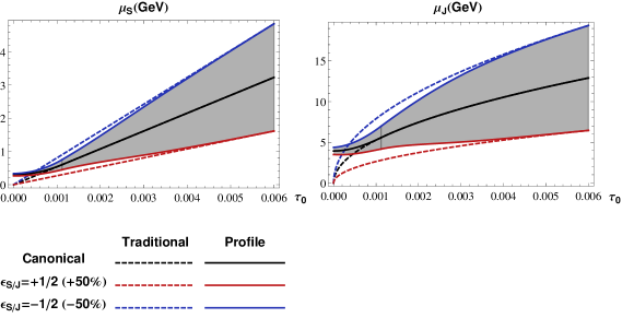
Figure 7: Profile functions for $\mu^{PF}_{S}(\tau_{0})$ and $\mu^{PF}_{J}(\tau_{0})$, the $\tau_{0}$-dependent renormalization scales that we use in the scale variations of our measured soft function and measured jet function. Also shown are traditional scale variations done by varying $\mu$ by $\pm 50\%$.

Here, we write down the profile functions used to perform scale variations for our measured soft and measured jet functions. We use profile functions to introduce a $\tau_{a}$-dependent scale variation that freezes at the characteristic scale for high values of $\tau_{a}$ where the factorization theorem breaks down and at a fixed scale for small values of $\tau_{a}$ where we reach the non-perturbative regime. The profile function for the measured soft function, $\mu_{S}^{PF}(\tau_{0})$, and the profile function for the measured jet function, $\mu_{J}^{PF}(\tau_{0})$, are plotted in Fig. 7 (for the case $a=0$). The analytic formulae for these functions are

$$\begin{split}\mu_{S}^{PF}(\tau_{a})=\left[1+\epsilon_{S}\frac{g(\tau_{a})}{g(1)}\right]\times\begin{cases}\mu_{min}+\alpha\tau_{a}^{\beta}\quad\quad&0<\tau_{a}<\tau_{min}\\ \omega\tau_{a}/r^{(1-a)}\quad\quad&\tau_{min}\leq\tau_{a}\\ \end{cases}\,,\\ \\ \mu_{J}^{PF}(\tau_{a})=\left[1+\epsilon_{J}\frac{g(\tau_{a})}{g(1)}\right]\times\begin{cases}(\omega r)^{(1-a)/(2-a)}(\mu_{min}+\alpha\tau_{a}^{\beta})^{1/(2-a)}\quad\quad&0<\tau_{a}<\tau_{min}\\ \omega\tau_{a}^{1/(2-a)}\quad\quad&\tau_{min}\leq\tau_{a}\end{cases}\,,\end{split}$$ (50)

where we have defined

$$g(\tau)=\frac{1}{\exp{\Big{(}1.26(\tau_{min}-\tau)/\tau_{min}\Big{)}}+1}\,,$$ (51)

and where $\alpha$ and $\beta$ are defined to be

$$\beta=\frac{\tau_{min}}{\tau_{min}-\mu_{min}r^{(1-a)}/\omega}\quad\text{and}\quad\alpha=\frac{\omega}{\beta\tau_{min}^{\beta-1}r^{(1-a)}}\,.$$ (52)

These choices for $\alpha$ and $\beta$ ensure that the profile functions and their first derivatives are continuous. We use the following values for the parameters

$$\tau_{min}=2\mu_{min}r^{1-a}/\omega$$

$$\mu_{min}=0.3\,{\rm GeV}\,.$$ (53)

We define our scale variations via

$$\begin{split}\epsilon_{S/J}=1/2\quad&\to\quad+50\%\text{\ variation},\\ \epsilon_{S/J}=-1/2\quad&\to\quad-50\%\text{\ variation},\\ \epsilon_{S/J}=0\quad&\to\quad\text{Canonical scale}\,,\end{split}$$

and take the final scale variation bands as the envelope of the set of bands from the individual variations.

Appendix B Matching Coefficients and Consistency Checks

B.1 Evaluation of matching coefficients

In pure dimensional regularization all diagrams contributing to the FFs vanish, and the only diagrams that contribute to the angularity FJF for quarks are Figs. 3a) and 3b) of Ref. Jain:2011xz . For Fig. 3a) we get

$$\frac{C_{F}\alpha_{s}}{2\pi}\frac{(4\pi\mu^{2})^{\epsilon}(1-\epsilon)}{\Gamma[1-\epsilon]}\frac{1-z}{1-a/2}\,\omega^{2a\epsilon/(2-a)}(1-z)^{-2(1-a)\epsilon/(2-a)}\\ \times\left(1+\frac{(1-z)^{1-a}}{z^{1-a}}\right)^{2\epsilon/(2-a)}\frac{1}{s_{a}^{1+2\epsilon/(2-a)}}\,,$$ (54)

and for Fig. 3b) we get

$$\frac{C_{F}\alpha_{s}}{2\pi}\frac{2z}{1-a/2}\frac{(4\pi\mu^{2})^{\epsilon}}{\Gamma[1-\epsilon]}\omega^{2a\epsilon/(2-a)}\frac{1}{(1-z)^{1+2(1-a)\epsilon/(2-a)}}\\ \times\left(1+\frac{(1-z)^{1-a}}{z^{1-a}}\right)^{2\epsilon/(2-a)}\frac{1}{s_{a}^{1+2\epsilon/(2-a)}}\,,$$ (55)

where $s_{a}=\omega^{2}\tau_{a}$. The first expression is singular as $\tau_{a}\to 0$ the second is singular as $z\to 1$ and $\tau_{a}\to 0$, but the singularities are regulated by dimensional regularization. Employing the distributional identity

$$\frac{1}{(1-z)^{1+\epsilon}}=-\frac{1}{\epsilon}\delta(1-z)+\left(\frac{1}{1-z}\right)_{+}-\epsilon\left(\frac{\ln(1-z)}{1-z}\right)_{+}+...\,,$$ (56)

and similarly for $\tau_{a}$ we find for the divergent terms

$$\frac{C_{F}\alpha_{s}}{2\pi}\Bigg{(}\delta(s_{a})\delta(1-z)\left[\frac{2-a}{1-a}\frac{1}{\epsilon^{2}}+\frac{2-a}{1-a}\frac{1}{\epsilon}\ln\left(\frac{\mu^{2}}{\omega^{2}}\right)+\frac{3}{2\epsilon}\right]\\ -\frac{1}{1-a}\frac{2}{\epsilon}\delta(1-z)\frac{1}{\omega^{2}}\left[\frac{1}{\tau_{a}}\right]_{+}-\delta(s_{a})\frac{1}{\epsilon}P_{qq}(z)\Bigg{)}\,,$$ (57)

where $P_{qq}$ is defined in Eq. (13). The first four terms in this expression are the expected UV poles for the angularity jet function (multiplied by $\delta(1-z)$), see Eq. (3.37) of Ref. Hornig:2009vb . In order to simplify this expression we have redefined $4\pi e^{-\gamma_{E}}\mu^{2}\to\mu^{2}$, i.e., we are working in the $\overline{MS}$ scheme. The last term is the expected UV pole in the perturbative evaluation of the QCD fragmentation function. Since ${\cal G}_{i}(\tau_{a},z,\mu)$ is expected to evolve like the angularity jet function, this is the correct structure of UV divergences implied by Eq. (2). The finite pieces are given by

$$\frac{1}{\omega^{2}}\frac{{\cal J}_{qq}(\tau_{a},z,\mu)}{2(2\pi)^{3}} =\frac{C_{F}\alpha_{s}}{2\pi}\frac{1}{\omega^{2}}\left\{\delta(\tau_{a})\delta(1-z)\frac{2-a}{1-a}\left(-\frac{\pi^{2}}{12}+\frac{1}{2}\ln^{2}\left(\frac{\mu^{2}}{\omega^{2}}\right)\right)\right.$$

$$+\delta(\tau_{a})\left(1-z-\left[\ln\left(\frac{\mu^{2}}{\omega^{2}}\right)+\frac{1}{1-a/2}\ln\left(1+\frac{(1-z)^{1-a}}{z^{1-a}}\right)\right]\frac{1+z^{2}}{(1-z)_{+}}\right.$$

$$+\left.\frac{1-a}{1-a/2}(1+z^{2})\left(\frac{\ln(1-z)}{1-z}\right)_{+}\right)$$

$$+\left[\frac{1}{\tau_{a}}\right]_{+}\left(\frac{1}{1-a/2}\frac{1+z^{2}}{(1-z)_{+}}-\delta(1-z)\frac{2}{1-a}\ln\left(\frac{\mu^{2}}{\omega^{2}}\right)\right)$$

$$\left.+\frac{2\delta(1-z)}{(1-a)(1-a/2)}\left[\frac{\ln\tau_{a}}{\tau_{a}}\right]_{+}\right\}\,.$$ (58)

In the limit $a\to 0$ this becomes

$$\begin{split}\frac{1}{\omega^{2}}\frac{{\cal J}_{qq}(\tau_{0},z,\mu)}{2(2\pi)^{3}}&=\frac{C_{F}\alpha_{s}}{2\pi}\left\{\delta(s)\delta(1-z)\left(-\frac{\pi^{2}}{6}+\ln^{2}\left(\frac{\mu^{2}}{\omega^{2}}\right)\right)\right.\\ &+\delta(s)\left(1-z-\ln\left(\frac{\mu^{2}}{\omega^{2}}\right)\frac{1+z^{2}}{(1-z)_{+}}+\ln z\,P_{qq}(z)+(1+z^{2})\left(\frac{\ln(1-z)}{1-z}\right)_{+}\right)\\ &\left.+\frac{1}{\omega^{2}}\left[\frac{1}{\tau_{0}}\right]_{+}\left(\frac{1+z^{2}}{(1-z)_{+}}-2\delta(1-z)\ln\left(\frac{\mu^{2}}{\omega^{2}}\right)\right)+2\delta(1-z)\frac{1}{\omega^{2}}\left[\frac{\ln\tau_{0}}{\tau_{0}}\right]_{+}\right\}\,,\end{split}$$ (59)

where we have used $\delta(\tau_{0})/\omega^{2}=\delta(s)$. Using the following distributional identities

$$\begin{split}\frac{1}{\omega^{2}}\left[\frac{1}{\tau_{0}}\right]_{+}&=\frac{1}{\omega^{2}}\left[\frac{\omega^{2}}{s}\right]_{+}=\frac{1}{\mu^{2}}\left[\frac{\mu^{2}}{s}\right]_{+}+\ln\left(\frac{\mu^{2}}{\omega^{2}}\right)\delta(s)\,,\\ \frac{1}{\omega^{2}}\left[\frac{\ln\tau_{0}}{\tau_{0}}\right]_{+}&=\frac{1}{\omega^{2}}\left[\frac{\ln(s/\omega^{2})}{s/\omega^{2}}\right]_{+}=\frac{1}{\mu^{2}}\left[\frac{\ln(s/\mu^{2})}{s/\mu^{2}}\right]_{+}+\frac{\ln(\mu^{2}/\omega^{2})}{\mu^{2}}\left[\frac{\mu^{2}}{s}\right]_{+}+\frac{1}{2}\ln\left(\frac{\mu^{2}}{\omega^{2}}\right)\delta(s)\,,\end{split}$$ (60)

which are readily verified by integrating both sides over $s$, one finds that in the $a\to 0$ limit the finite piece is given by

$$\frac{{\cal J}_{qq}(s,z,\mu)}{2(2\pi)^{3})} =\frac{C_{F}\alpha_{s}}{2\pi}\left\{\delta(s)\left(1-z+\ln z\,P_{qq}(z)+(1+z^{2})\left(\frac{\ln(1-z)}{1-z}\right)_{+}-\frac{\pi^{2}}{6}\delta(1-z)\right)\right.$$

$$\left.+\frac{1}{\mu^{2}}\left[\frac{\mu^{2}}{s}\right]_{+}\frac{1+z^{2}}{(1-z)_{+}}+2\delta(1-z)\frac{1}{\mu^{2}}\left[\frac{\ln(s/\mu^{2})}{s/\mu^{2}}\right]_{+}\right\}\,,$$ (61)

which agrees with the matching coefficient found in Eq. (2.32) of Ref. Jain:2011xz .

Next we calculate ${\cal J}_{qg}(\tau_{a},z,\mu)$. Naively this is related to ${\cal J}_{qq}(\tau_{a},z,\mu)$ by the replacement $z\to 1-z$. However, because in the convolution integral of Eq. (2) the argument of ${\cal J}_{ij}(\tau_{a},z/z^{\prime},\mu)$ is never zero, there is no need to regulate poles of $z$. Therefore, a divergent factor of $(1-z)^{-1-\epsilon}$ in ${\cal J}_{qq}(\tau_{a},z,\mu)$ becomes in ${\cal J}_{qg}(\tau_{a},z,\mu)$

$$\frac{1}{z^{1+\epsilon}}=\frac{1}{z}-\epsilon\frac{\ln z}{z}+O(\epsilon^{2})\,.$$ (62)

Thus, ${\cal J}_{qg}(\tau_{a},z,\mu)$ is obtained by making the substitution $z\to 1-z$ and then dropping all $\delta(z)$ and plus prescriptions. This is true for the ${\cal J}_{qg}(s,z,\mu)$ calculated in Ref. Jain:2011xz and remains true for ${\cal J}_{qg}(\tau_{a},z,\mu)$. We thus find for the divergent terms

$$\frac{1}{\omega^{2}}\frac{{\cal J}^{div}_{qg}(\tau_{a},z,\mu)}{2(2\pi)^{3}}=-\frac{1}{\omega^{2}}\frac{C_{F}\alpha_{s}}{2\pi}\frac{1}{\epsilon}\delta(\tau_{a})P_{gq}(z)\,,$$ (63)

where $P_{gq}$ is given in Eq. (13). For the finite pieces we get

$$\begin{split}\frac{1}{\omega^{2}}\frac{{\cal J}_{qg}(\tau_{a},z,\mu)}{2(2\pi)^{3}}&=\frac{C_{F}\alpha_{s}}{2\pi}\frac{1}{\omega^{2}}\Bigg{\{}\delta(\tau_{a})\Big{(}z+\Big{[}\frac{1}{1-a/2}\ln\left(\frac{z^{1-a}(1-z)^{1-a}}{z^{1-a}+(1-z)^{1-a}}\right)\\ &-\ln\left(\frac{\mu^{2}}{\omega^{2}}\right)\Big{]}P_{gq}(z)\Big{)}+\frac{1}{1-a/2}\left[\frac{1}{\tau_{a}}\right]_{+}P_{gq}(z)\Bigg{\}}\,.\end{split}$$ (64)

Again, these reproduce the matching coefficients of Ref. Jain:2011xz in the $a\to 0$ limit.

For the divergent contributions to ${\cal J}_{gg}(\tau_{a},z,\mu)$ we get (from the diagrams in Fig. 4 of Ref. Jain:2011xz )

$$\frac{1}{\omega^{2}}\frac{\mathcal{J}^{div}_{gg}(\tau_{a},z,\mu)}{2(2\pi)^{3}} =\frac{C_{A}\alpha_{s}}{2\pi}\frac{1}{\omega^{2}}\Bigg{(}\delta(\tau_{a})\delta(1-z)\left[\frac{2-a}{1-a}\frac{1}{\epsilon^{2}}+\frac{2-a}{1-a}\frac{1}{\epsilon}\ln\left(\frac{\mu^{2}}{\omega^{2}}\right)+\frac{\beta_{0}}{2C_{A}}\frac{1}{\epsilon}\right]$$

$$-\frac{1}{1-a}\frac{2}{\epsilon}\delta(1-z)\left[\frac{1}{\tau_{a}}\right]_{+}\Bigg{)}-\frac{\alpha_{s}}{2\pi}\frac{1}{\omega^{2}}\delta(\tau_{a})\frac{1}{\epsilon}\tilde{P}_{gg}(z)\,,$$ (65)

where the $\tilde{P}_{gg}(z)$ is the ${\bf full}$ QCD splitting function that includes the term proportional to $\beta_{0}\delta(1-z)$. For the finite parts of ${\cal J}_{gg}(\tau_{a},z,\mu)$ we find

$$\frac{1}{\omega^{2}}\frac{{\cal J}_{gg}(\tau_{a},z,\mu)}{2(2\pi)^{3}} = \frac{C_{A}\alpha_{s}}{2\pi}\frac{1}{\omega^{2}}\left\{\delta(\tau_{a})\delta(1-z)\frac{2-a}{1-a}\left(-\frac{\pi^{2}}{12}+\frac{1}{2}\ln^{2}\left(\frac{\mu^{2}}{\omega^{2}}\right)\right)\right.$$ (66)

$$+\delta(\tau_{a})\left(-P_{gg}(z)\left[\ln\left(\frac{\mu^{2}}{\omega^{2}}\right)+\frac{1}{1-a/2}\ln\left(1+\frac{(1-z)^{1-a}}{z^{1-a}}\right)\right]\right.$$

$$+\left.\frac{1-a}{1-a/2}\frac{2(1-z+z^{2})^{2}}{z}\left(\frac{\ln(1-z)}{1-z}\right)_{+}\right)$$

$$+\left[\frac{1}{\tau_{a}}\right]_{+}\left(\frac{1}{1-a/2}P_{gg}(z)-\delta(1-z)\frac{2}{1-a}\ln\left(\frac{\mu^{2}}{\omega^{2}}\right)\right)$$

$$\left.+\frac{2\delta(1-z)}{(1-a)(1-a/2)}\left[\frac{\ln\tau_{a}}{\tau_{a}}\right]_{+}\right\}\,,$$

where $P_{gg}$ is given in Eq. (13). In the limit $a\to 0$, this expression reduces to ${\cal J}_{gg}(s,z,\mu)/(16\pi^{3})$ found in Eq. (2.33) of Ref. Jain:2011xz .

For the divergent contributions to ${\cal J}_{gq}(\tau_{a},z,\mu)$ we find

$$\frac{1}{\omega^{2}}\frac{{\cal J}^{div}_{gq}(\tau_{a},z,\mu)}{2(2\pi)^{3}} = -\frac{1}{\omega^{2}}\frac{\alpha_{s}T_{R}}{2\pi}\frac{1}{\epsilon}\delta(\tau_{a})P_{qg}(z)\,.$$ (67)

For the finite parts we get

$$\frac{1}{\omega^{2}}\frac{{\cal J}_{gq}(\tau_{a},z,\mu)}{2(2\pi)^{3}} = \frac{\alpha_{s}T_{R}}{2\pi}\frac{1}{\omega^{2}}\left\{\frac{1}{1-a/2}\left[\frac{1}{\tau_{a}}\right]_{+}P_{qg}(z)+\delta(\tau_{a})2z(1-z)\right.$$

$$\left.+\,\delta(\tau_{a})P_{qg}(z)\left[\frac{1}{1-a/2}\ln\left(\frac{z^{1-a}(1-z)^{1-a}}{z^{1-a}+(1-z)^{1-a}}\right)-\ln\left(\frac{\mu^{2}}{\omega^{2}}\right)\right]\right\}\,,$$

where $P_{qg}$ is again given in Eq. (13). In the limit $a\to 0$, this expression reduces to ${\cal J}_{gq}(s,z,\mu)/(16\pi^{3})$ in Eq. (2.33) of Ref. Jain:2011xz .

B.2 Sum Rules

The sum rules,

$$J_{i}(\tau_{a}) =\frac{1}{2(2\pi)^{3}}\sum_{j}\int_{0}^{1}dz\,z\,\mathcal{J}_{ij}(\tau_{a},z)\,,$$ (69)

can be checked for $i=q$ by performing the integral

$$J_{q}(\tau_{a}) =\frac{1}{2(2\pi)^{3}}\sum_{j}\int_{0}^{1}dz\,z\,{\cal{J}}_{qj}(\tau_{a},z)$$ (70)

$$=\frac{1}{2(2\pi)^{3}}\int_{0}^{1}dz\,z\,\left(\mathcal{J}_{qq}(\tau_{a},z)+\mathcal{J}_{qg}(\tau_{a},z)\right)$$ (71)

$$=\frac{1}{2(2\pi)^{3}}\int_{0}^{1}dz\,z\,\left(\mathcal{J}_{qq}(\tau_{a},z)+\mathcal{J}_{qq}(\tau_{a},1-z)\right)$$ (72)

$$=\frac{1}{2(2\pi)^{3}}\int_{0}^{1}dz\,\mathcal{J}_{qq}(\tau_{a},z),$$ (73)

where in the last line we changed variables to $z\to 1-z$ in the 2nd term. Inserting the expression in Eq. (B.1) into this integral yields the $J_{q}(\tau_{a})$ found in Eq. (3.35) of Ref. Hornig:2009vb .

In the case of the $i=g$ we have

$$J_{g}(\tau_{a}) =\frac{1}{2(2\pi)^{3}}\int_{0}^{1}dz\,z\,\left(\mathcal{J}_{gg}(\tau_{a},z)+\mathcal{J}_{gq}(\tau_{a},z)\right)\,$$

$$=\frac{1}{2(2\pi)^{3}}\int_{0}^{1}dz\,\frac{\mathcal{J}_{gg}(\tau_{a},z)+\mathcal{J}_{gq}(\tau_{a},z)}{2}\,,$$ (74)

because both $\mathcal{J}_{gg}(\tau_{a},z)$ and $\mathcal{J}_{gq}(\tau_{a},z)$ are symmetric under $z\to 1-z$. The sum rule is easiest to verify by writing the $d$-dimensional expressions for $\mathcal{J}_{gg}(\tau_{a},z)$ and $\mathcal{J}_{gq}(\tau_{a},z)$ before expanding in $\epsilon=(4-d)/2$. We find

$$\frac{1}{\omega^{2}}\frac{\mathcal{J}_{gg}(\tau_{a},z,\mu)}{2(2\pi)^{3}} = \frac{1}{\omega^{2}}\left(\frac{4\pi\mu^{2}}{\omega^{2}}\right)^{\epsilon}\frac{C_{A}\alpha_{s}}{2\pi}\frac{1}{\Gamma[1-\epsilon]}\frac{1}{1-a/2}(z^{a-1}+(1-z)^{a-1})^{\frac{2\epsilon}{2-a}}\left(\frac{1}{\tau_{a}}\right)^{1+\frac{2\epsilon}{1-a}}$$ (75)

$$\times \left(\frac{2z}{1-z}+\frac{2(1-z)}{z}+2z(1-z)\right)$$

$$\frac{1}{\omega^{2}}\frac{\mathcal{J}_{gq}(\tau_{a},z,\mu)}{2(2\pi)^{3}} = \frac{1}{\omega^{2}}\left(\frac{4\pi\mu^{2}}{\omega^{2}}\right)^{\epsilon}\frac{T_{R}\alpha_{s}}{2\pi}\frac{1}{\Gamma[1-\epsilon]}\frac{1}{1-a/2}(z^{a-1}+(1-z)^{a-1})^{\frac{2\epsilon}{2-a}}\left(\frac{1}{\tau_{a}}\right)^{1+\frac{2\epsilon}{1-a}}$$ (76)

$$\times \left(1-\frac{2}{1-\epsilon}z(1-z)\right)\,.$$

Inserting these two expressions into Eq. (B.2) one obtains exactly the integral expression for the $d$-dimensional $J_{g}(\tau_{a})$ found in Eq. (4.22) of Ref. Ellis:2010rwa .