Magnetic field-dependent inhomogeneities and their effect on the magnetoresponse of 2D superconductors

Abstract

We show that inhomogeneities in the spatial distribution of Cooper pairs and in the phase of the local superconducting order parameter in the vicinity of a superconductor-normal state transition (SNT) in two dimensions can be highly sensitive to a perpendicular magnetic field. We focus on the role of orbital effects in the field-dependence of local superfluid stiffness and superconducting phase disorder in homogeneously-disordered two-dimensional superconductor thin films. The relative importance of these orbital effects is analyzed in different physical regimes dominated by Coulomb blockade, thermal phase fluctuations and Aharanov-Bohm phase disorder respectively. Following this approach, we obtain explicit expressions for the field dependence of magnetoresistance and superfluid stiffness near the SNT, and attempt an understanding of some recent experimental findings.

One of the most challenging problems in strongly disordered superconductors relates to understanding the nature of the magnetic field-induced superconductor-normal state transition (SNT). Experimental and theoretical studies over the past two decades have opened a large number of puzzling questions such as the origin of the giant non-monotonous magnetic field dependence of the resistivity Sambandamurthy et al. (2004); Steiner et al. (2005); Shangina and Dolgopolov (2003); Dubi et al. (2006); Pokrovsky et al. (2010); Galitski et al. (2005); Lopatin and Vinokur (2007), flux quantization in the insulating state Stewart et al. (2007) and the universality class governing the field-induced SNT Breznay et al. (2016); Paalanen et al. (1992); Fisher (1990); Shangina and Dolgopolov (2003). The two-dimensional (2D) case has in particular attracted intense theoretical attention and it is the focus of this work. In the absence of a magnetic field, it is well-known that strong homogeneous disorder introduces granularity in the form of superconducting islands embedded in an insulating matrix Ioffe and Larkin (1981); Fisher et al. (1989); Ghosal et al. (1998); Sacépé et al. (2008); Chand et al. (2012). However the role of an external magnetic field on the SNT through its effect on the distribution of such islands Pokrovsky et al. (2010); Dubi et al. (2006) and on the associated phase frustration brought in by the Aharonov-Bohm (AB) phases of the Cooper pairs tunneling across the islands Chakrabarti and Dasgupta (1988); Kim and Stroud (2008) is not well-understood and is a topic of considerable current debate.

Mean-field analyses of the field-sensitivity of the distribution of superconducting regions go back nearly two decades for weakly-disordered metals Spivak and Zhou (1995); Galitski and Larkin (2001), and more recently, Dubi et al. (2006) for strongly-disordered insulators. Standard, perturbative approaches fail in the strongly-disordered regime but numerical mean-field solutions of the appropriate Bogoliubov – de Gennes (BdG) equations Dubi et al. (2006) reveal a picture of shrinking superconducting regions in increasing fields, a downward shift of the distribution of the local superconducting gaps, and through the Ambegaokar-Baratoff relation Ambegaokar and Baratoff (1963), a corresponding decrease in the Josephson couplings $J$ between neighboring grains. To understand the physical origin of these effects, we study a phenomenological model of repulsive bosons (Cooper pairs) subjected to a disordered potential and a perpendicular magnetic field. The approach is reminiscent of earlier work on Lifshitz states Lifshitz (1968) in disordered Bose systems Larkin and Vinokur (1995); Falco et al. (2009); Pokrovsky et al. (2010). We obtain the typical size and separation of the superconducting islands and show that wave function shrinking in the presence of a magnetic field suppresses the Josephson couplings as $J(B)\sim\exp[-(B/B_{J})^{2}].$

To understand magnetoresponse of these 2D granular superconductors, we study the standard Josephson-junction (XY) model,

$$L =\frac{1}{4E_{c}}\sum_{\mathbf{i}}(\partial_{\tau}\phi_{\mathbf{i}})^{2}-\sum_{\langle\mathbf{ij}\rangle}J_{\mathbf{ij}}(B)\cos(\phi_{\mathbf{ij}}+A_{\mathbf{ij}}),$$ (1)

where $E_{c}$ represents the Coulomb blockade scale, $\phi_{\mathbf{ij}}=\phi_{\mathbf{i}}-\phi_{\mathbf{j}}$ is the superconducting phase difference between neighboring grains at positions $\mathbf{i}$ and $\mathbf{j}$ respectively, and $A_{\mathbf{ij}}=(2e/\hbar)\int_{\mathbf{i}}^{\mathbf{j}}\mathbf{A}\cdot d\mathbf{r}$ are the AB phases acquired by the hopping Cooper pairs. Disregarding the contribution of normal quasi particles means the model can provide a good description of the magnetoresponse only at lower fields where Cooper pair breaking is not important. Spatial disorder in the grain positions introduces randomness in the Josephson couplings as well as the AB phases. Studies of the 2D classical limit of Eq.(1) in the $B=0$ limit Dubi et al. (2006) have shown that strong disorder in $J$ does not alter the universality class of the SNT from the homogeneous case (where it is known to be of Kosterlitz-Thouless (KT) type) but is nevertheless dominated by a percolating backbone of paths with the largest local superfluid stiffnesses. Likewise the transition in the quantum 1D disordered counterpart at $B=0$ also falls in the KT universality class Altman et al. (2004); Giamarchi and Schulz (1988). Therefore for simplicity we will work with the typical value of $J$ ignoring its spatial disorder.

In regular lattices, the AB phase is associated with flux threading the plaquettes, and depending on the amount of frustration $f$ (measured as a fraction of a flux quantum), leads to oscillations in properties such as the critical current and the resistance Teitel and Jayaprakash (1983); Van der Zant et al. (1996). Such matching (commensuration) effects are absent in the disordered case as there is random flux penetration in different plaquettes. In a phenomenal work, Carpentier and Le Doussal Carpentier and Le Doussal (2000, 1998) studied phase transitions in the classical quenched random phase XY model on a square lattice close to integer $f.$ The presence of disorder results in rare favorable regions for the occurrence of vortices at low temperatures. At sufficiently low temperatures, they found that the disorder-induced phase transition is not in the KT universality class. Very similar results were also obtained earlier Giamarchi and Schulz (1988) in a study of the Anderson localization in one-dimensional Luttinger-liquids subjected to quenched phase disorder. The similarity is puzzling since quenched disorder in 1D is equivalent to columnar disorder in the two-dimensional case. Quantum Monte Carlo studies Kim and Stroud (2008) of the interplay of phase frustration and Coulomb blockade suggest a zero temperature field-driven SNT with dynamic exponent $z\approx 1.3,$ placing the transition in a different universality class from 3D XY.

In this Letter we study the effect of three dominant mechanisms governing loss of phase coherence and their specific signatures on the magnetoresistance and superfluid stiffness. These are (a) quantum phase fluctuations originating from Coulomb blockade, (b) thermal fluctuations of the phase and (c) frustration effects due to disorder in AB phases. We show that Coulomb blockade effects impart a specific signature to the magnetoresistance, $\rho(B)\sim\exp[(B/B_{0})^{2}].$ Where the SNT is driven by thermal fluctuations, we find a KT transition, with $\rho(B)\sim\exp[-1/\sqrt{B-B_{KT}}]$ in the critical region. In the AB phase frustration dominated regime, we find a new, non KT critical behavior, $\rho(B)\sim\exp[-1/(B-B_{AB})].$ The field-dependent superfluid stiffness $\Upsilon$ also shows a surprising behavior: at small fields, we find that phase frustration effects on $\Upsilon$ are more significant than the field dependence of Josephson couplings. In the Coulomb blockade regime away from the critical region, our predicted magnetoresistance is in excellent accord with experimental data Sambandamurthy et al. (2004); Steiner et al. (2005). However in the critical scaling region, existing experimental data is somewhat less clear, and while there is some evidence for mechanism (c) for the field-tuned SNT in oxide heterostructuresBiscaras et al. (2013) , further study is needed and we propose additional probes to distinguish between the two.

We now analyze the effect of a transverse magnetic field on the distribution of the SC islands in the granular superconductor. Consider a model of repulsive bosons (Cooper pairs) with average density $n$ subjected to a random potential with a Gaussian white noise distribution:

$$H =\sum_{\mathbf{p}}\frac{\Pi^{2}}{2m}a_{\mathbf{p}}^{\dagger}a_{\mathbf{p}}+\int_{\mathbf{r}}\left[\frac{g}{2}|\Psi(\mathbf{r})|^{4}+U(\mathbf{r})|\Psi(\mathbf{r})|^{2}\right],$$ (2)

where $\Psi(\mathbf{r})=\frac{1}{\sqrt{V}}\sum_{\mathbf{p}}a_{\mathbf{p}}\exp[i\mathbf{p}\cdot\mathbf{r}/\hbar],$ $\Pi=(\mathbf{p}-q\mathbf{A}),$ $U(\mathbf{r})$ is the random potential, $\langle U(\mathbf{r})\rangle=0$ and $\langle U(\mathbf{r})U(\mathbf{r}^{\prime})\rangle=\kappa^{2}\delta(\mathbf{r}-\mathbf{r}^{\prime}),$ $q=2e$ is the boson charge and $g,$ parametrizes the boson repulsion. We choose the gauge $\mathbf{A}=\frac{1}{2}(\mathbf{B}\times\mathbf{r})$ with the field in the transverse $z$ direction. This model is equivalent to earlier studied (for $B=0$) Ginzburg-Landau models with disorder in critical temperature Ioffe and Larkin (1981). The important length scales in the model are the single particle localization length ${\cal L}=\hbar^{2}/m\kappa$ characterizing the disorder, and the magnetic length $l_{B}\sim\sqrt{e/(2\pi\hbar B}).$ We are specifically interested in the regime ${\cal L}/l_{B}\ll 1.$ At low densities, the interplay of disorder and interpaticle repulsion leads to the formation of disconnected islands of localized bosons Falco et al. (2009) whose typical size and separation may be estimated as follows. The optimal potential fluctuation that has a bound state at energy $E<0$ is found by minimizing $\frac{1}{2}\int U^{2}d\mathbf{r}+\lambda(E-H),$ where $\lambda$ is a Lagrange multiplier. We choose $\Psi$ to be real, assuming a spherical fluctuation and zero angular momentum bound state. Varying with respect to $U,$ we obtain $U=\lambda\Psi^{2};$ thus the size $R$ of the optimum potential well is also of the same order as the wave function. The energy of a particle in an island, in the mean-field approximation, is thus of the order of $-\frac{\hbar^{2}}{2mR^{2}}+\frac{(qBR)^{2}}{8m}+gN_{p}/(\pi R^{2}),$ where $N_{p}$ is the number of bosons in the island. The density $n_{w}=n/N_{p}$ of these islands is determined by the Gaussian factor, $\exp[-\frac{1}{2\kappa^{2}}\int_{\mathbf{r}}U^{2}],$ whence $n_{w}\sim(1/\pi R)^{2}\exp[-(\hbar^{2}/m\kappa R)^{2}]=(1/\pi R)^{2}\exp[-({\cal L}/R)^{2}].$ Minimizing the energy with respect to $R,$ the size of the typical island, to logarithmic precision, is

$$R(B) \sim\frac{{\cal L}}{\sqrt{\ln[n_{c}(B)/n]}},$$ (3)

where $n_{c}(B)\approx\frac{\hbar^{2}}{2gm{\cal L}^{2}}\left(1+\frac{(qB{\cal L}^{2}/\hbar)^{2}}{4}\frac{1}{\ln^{2}(n_{c}(0)/n)}\right)$ for small fields, is the critical density for percolation of the islands and $n_{c}(B)/n>1.$ For future convenience we introduce $w(B)=n_{c}(B)/n.$ Clearly the magnetic field shrinks the islands but the field-dependence is very different from a simple expectation from wave function shrinking of a localized noninteracting particle. The distance $D\sim 1/\sqrt{n_{w}}$ between the islands can be estimated as $D(B)\sim R(B)e^{\frac{1}{2}({\cal L}/R(B))^{2}}\sim{\cal L}\sqrt{w(B)},$ whence, on account of the exponential dependence of inter-island tunneling probability, the typical inter-island Josephson coupling behaves as $J\sim e^{-2D(B)/R(B)}$

$$J(B) \sim e^{-2\sqrt{w(B)}}.$$ (4)

Note that even when at small magnetic fields, ${\cal L}/l_{B}\ll 1,$ the exponent in Eq. 4 can be large at low boson densities, $w(B)\gg 1.$ For such fields we have $J(B)/J(0)\sim e^{-(B/B_{J})^{2}},$ where $B_{J}^{-2}\approx\frac{\sqrt{w(0)}}{\ln^{2}w(0)}(q{\cal L}^{2}/2\hbar)^{2}.$ We now analyze the effects of the three different mechanisms that lead to loss of global phase coherence in their regimes of dominance which are determined by the dimensionless parameters $E_{c}/J,$ $T/J$ and $\sigma,$ with the latter a measure of disorder in the fluxes through elementary plaquettes. Figure 1 shows the phase diagram and the regimes of our study.

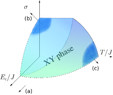
Figure 1: Schematic phase diagram for the 2D superconductor-normal state transition, with the XY superfluid phase in the interior of the surface, as a function of dimensionless temperature $T/J,$ Coulomb blockade scale $E_{c}/J$ and the Aharanov-Bohm (AB) phase disorder $\sigma$ for the model described in Eq. (1). Here $J$ is the (field-dependent) Josephson coupling estimated in the paper. (a) refers to the Coulomb blockade dominated regime. The shaded regions (b) and (c) denote transitions driven by AB phase frustration and thermal phase fluctuation respectively. The dotted line on the surface separates these two different critical scaling regimes. The critical disorder at low $T$ and $E_{c}$ is independent of $T$ and scaling of the correlation length is not of the Kosterlitz-Thouless type Carpentier and Le Doussal (2000).

(a) Quantum phase fluctuations dominated insulating regime ($E_{c}/J,\,E_{c}/T\gg 1$) : We treat the Josephson term in Eq.(1) as a perturbation, and calculate the conductivity using the Kubo formula Tripathi and Loh (2006); Syzranov et al. (2009). Transport in this model proceeds through Arrhenius activation and incoherent sequential hopping of charges between neighboring islands - this leads to a resistivity of the form

$$\rho(B) \sim J(B)^{-2}e^{E_{c}(B)/T}\sim e^{[4\sqrt{w(B)}+(q^{2}/{\cal L}T)\sqrt{\ln w(B)}]}.$$ (5)

The above behavior shows the insulating nature of the normal state. For small fields, the magnetoresistance obeys the law $\rho(B)/\rho(0)\sim\exp[(B/B_{0})^{2}],$ where $B_{0}^{-2}\approx\frac{(q{\cal L}^{2}/2\hbar)^{2}}{2\ln^{2}w(0)}[\sqrt{w(0)}+\frac{q^{2}}{{\cal L}T\sqrt{\ln w(0)}}].$ More accurately, one must also take into account the renormalization of the charging energy by Josephson coupling Syzranov et al. (2009); Fistul et al. (2008), $E_{c}\rightarrow E_{c}-J.$ It is interesting to note that a similar field dependence of resistivity $\rho(B)\sim e^{(B/B_{c}-1)^{2}}$ has been obtained in the context of a superconductor to Hall insulator transition Shimshoni et al. (1998).

(b) AB phase frustration dominated regime ($E_{c}/J\ll 1,\,T/J\ll 1,\,\sigma/\sigma_{c}\sim 1$): To study this regime, it is useful to consider the Coulomb gas representation of the model in Eq. (1). Following earlier works Carpentier and Le Doussal (2000); Petković et al. (2009) we assume a Gaussian white noise distribution for the AB phases on the links, reckoned from a background average corresponding to a typical separation of islands, $D.$ In the Coulomb gas representation, such disorder translates to a random flux threading elementary plaquettes, corresponding to an external potential $V_{\mathbf{r}}$ acting on the “charges” (vortices) with a Gaussian distribution $\langle(V_{\mathbf{r}}-V_{\mathbf{r}^{\prime}})^{2}\rangle=4\sigma J^{2}\ln|\mathbf{r}-\mathbf{r}^{\prime}|+O(1).$ Denoting the plaquette area fluctuation by $(\delta D)^{2},$ we identify $\sigma\sim B^{2}(\delta D)^{4}.$ It is crucial that the random background potential has long-range (logarithmic) correlations. In the continuum description of the model with a lower cutoff scale $a_{0},$ $V_{\mathbf{r}}$ has a local part $v_{\mathbf{r}}:\,\langle(v_{\mathbf{r}}-v_{\mathbf{r}^{\prime}})^{2}\rangle\sim\sigma J^{2}$ and a long-range correlated part $V_{\mathbf{r}}^{>}$ with no cross-correlation between these two parts. The Coulomb gas Hamiltonian then reads

$$H =-J\sum_{\mathbf{r}\neq\mathbf{r}^{\prime}}n_{\mathbf{r}}n_{\mathbf{r}^{\prime}}\ln\left(\frac{|\mathbf{r}-\mathbf{r}^{\prime}|}{a_{0}}\right)-\sum_{\mathbf{r}}\left[n_{\mathbf{r}}V_{\mathbf{r}}^{>}-\ln Y[n_{\mathbf{r}},\mathbf{r}]\right],$$ (6)

where $n_{\mathbf{r}}$ represents integer charge at $\mathbf{r}$ and the spatially dependent fugacities have the bare value, $\ln Y[n_{\mathbf{r}},\mathbf{r}]=\gamma Jn_{\mathbf{r}}^{2}+n_{\mathbf{r}}v_{\mathbf{r}},$ and $\gamma$ is a constant of order unity. We have dropped the background term as it just sets the chemical potential of the vortices and does not affect the scaling equations Oganesyan et al. (2006).

In the absence of disorder, the usual RG procedure consists of (i) increasing the short scale cutoff, $a_{0}\rightarrow a_{0}+dl,$ and eliminating all dipoles in the annulus of thickness $dl,$ and (ii) disregard all configurations that increase the net charge within the cutoff region. The RG procedure is perturbatively controlled by small dipole fugacities. For the disordered case, we follow Ref.Carpentier and Le Doussal (2000) and introduce replicas which allows us to perform the average over Gaussian disorder. The lowest excitations continue to carry charges $0,\,\pm 1$ but now the $n_{\mathbf{r}}^{\alpha}$ also carry a replica index $\alpha.$ An important difference from the RG procedure of the disorder-free case is that now when the cutoff is increased, one must, apart from considering annihilation of replica charges, also take into account “fusion” of unit charges in different replicas (see appendix). Another important difference that invalidates the usual perturbative expansion in small dipole fugacities is that the random potential creates favorable regions for single vortex formation. Hence we study the scale dependence of the single vortex fugacity distribution identifying the density of rare favorable regions, $\rho_{a_{0}}^{v},$ for the occurrence of vortices as the perturbation parameter. By studying the scaling of $\rho_{a_{0}}^{v},$ two distinct regimes can be identified for $T/J\ll 1$: (a) an XY phase phase at sufficiently low bare disorder where $\rho_{a_{0}}^{v}$ scales to zero, and (b) a disordered phase beyond a critical bare disorder where $\rho_{a_{0}}^{v}$ diverges (see appendix for details). In the disordered phase, the phase correlation length has a surprising non-KT behavior, $\xi\sim e^{1/(\sigma-\sigma_{c})},$ which in our context translates to a field dependence $\xi\sim e^{1/(B-B_{AB})},$ with $B_{AB}\sim\hbar/q(\delta D)^{2}.$ Such a non-KT behavior is a direct consequence of the logarithmic scaling of the disorder potential correlations. Another peculiarity is that over a range of low temperatures up to a scale of order $J,$ the critical disorder $\sigma_{c}$ is independent of the temperature Carpentier and Le Doussal (2000).

We obtain the magnetic field dependence of the superfluid stiffness by solving the scaling equations in the critical region at low temperatures for the coupling constant $J_{l}$ and the effective disorder $\sigma_{l}.$ Taking the ratio of the scaling equations for $J_{l}$ and $\sigma_{l}$ obtained in Ref.Carpentier and Le Doussal (2000), we get

$$\frac{\partial_{l}J_{l}^{-1}}{\partial_{l}\sigma_{l}} \sim\frac{1}{J_{l}\sqrt{\sigma_{l}}},$$

and from the solution $J_{l}\sim e^{-2\sqrt{\sigma_{l}}}$ it follows that the superfluid stiffness $\Upsilon(B)$ has the behavior

$$\Upsilon(B) \sim J(B)e^{-2\sqrt{\sigma(B)}}\sim e^{-(B/B_{1})-(B/B_{J})^{2}},$$ (7)

where $B_{1}$ is of the order of $B_{AB}.$ Phase frustration effects thus play a more important role in determining the low-field dependence of superfluid stiffness in the AB phase-frustration dominated regime compared to the effect coming from orbital shrinking.

Now we analyze magnetoresistance in the disordered phase at low temperatures and close to the field-induced transition. Following Halperin and Nelson Halperin and Nelson (1979) we estimate the electrical resistivity (which is essentially the vortex conductivity) as $\rho(B)=\mu_{v}n(B),$ where $\mu_{v}$ is the temperature and field-dependent mobility of the vortices, and $n(B)\sim 1/\xi^{2}$ is the vortex density. We make an assumption that $\mu_{v}(B)$ is well-behaved near $B=B_{AB},$ which allows us to neglect its field dependence in comparison to the singular behavior of $\xi(B).$ The temperature dependence of resistivity is governed by the temperature dependence of the mobility, and we believe it shows an activated behavior given the logarithmic Coulomb interaction of the vorticesShklovskii (2008). The magnetoresistance in this AB phase frustration dominated regime thus grows as

$$\rho(B) \sim\mu_{v}(T)e^{-1/(B-B_{AB})}.$$ (8)

(c) Thermal phase fluctuations dominated KT regime ($E_{c}/J\ll 1,\,\sigma/\sigma_{c}\ll 1,\,T/J(B)\sim 1$): In this regime, the transition is brought about by the proliferation of thermally activated vortices. The superfluid stiffness now has a field dependence$\Upsilon(B)\sim J(B)\sim e^{-(B/B_{J})^{2}}$ arising from orbital shrinking of the superconducting islands. For the resistivity we again consider the correlation length in the disordered phase, which has the well-known form, $\xi\sim e^{1/\sqrt{T-T_{KT}}},$ with $T_{KT}\propto J(B).$ Near the transition, this is equivalent to a field-dependent correlation length, $\xi\sim e^{1/\sqrt{B-B_{KT}}}.$ Thus the resistivity in this regime has the form

$$\rho(B) \sim\mu_{v}(T)e^{-1/\sqrt{B-B_{KT}}}.$$ (9)

For regimes (b) and (c), the normal state has a “metallic” temperature dependence since enhancement of vortex mobilities at higher temperatures translates to higher resistivity.

Relation to experiments: Figure 2 shows the low-temperature and low-field magnetoresistance of disordered InO_x thin films extracted from two different experiments Sambandamurthy et al. (2004); Steiner et al. (2005). The positive magnetoresistance data is very well-described by Eq. (5) which places these samples in our Coulomb blockade dominated regime. Deviation from the Coulomb blockade prediction is seen near the magnetoresistance peak and we believe this is due to the quasi particle transport channel opening up. In samples with lower disorder Steiner et al. (2005), unsurprisingly, Coulomb blockade does not adequately explain the data; however, the other critical scaling regimes (AB phase frustration and KT) show better agreement even though we were unable to distinguish between the two (see appendix). In a recent study of the field-tuned SNT at 2D interfaces of gated oxide heterostructures Biscaras et al. (2013), it was reported that for certain gate voltages, the critical magnetic field at low temperatures was independent of the temperature, suggestive of the phase frustration driven SNT mechanism. Finally, our predictions for superfluid stiffness in the XY regime can possibly be tested through studies of field-dependent ac conductivityMisra et al. (2013) and may provide an independent means for distinguishing between the two regimes in the XY phase.

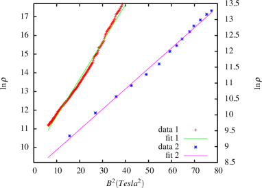
Figure 2: Resistivity $\rho$ as a function of perpendicular magnetic field $B$ for disordered InO_x thin films as reported in Ref.Sambandamurthy et al. (2004) (data 1) and Ref. Steiner et al. (2005) (data 2) in the low-field region where the fits are to the predicted behavior $\rho(B)\sim e^{(B/B_{0})^{2}}$ corresponding to the Coulomb blockade dominated regime discussed in the text.

In summary, we studied the field-dependence of the distribution of SC islands in strongly disordered superconductors and constructed an effective Josephson-junction model with field-dependent parameters. Analyzing the model in different physical regimes - dominated by Coulomb blockade, thermal phase fluctuations or Aharanov-Bohm phase fluctuations - we obtained the field-dependence of resistivity and superfluid stiffness. In the Coulomb blockade regime, available experimental data is in excellent agreement with our prediction $\rho(B)\sim e^{(B/B_{0})^{2}},$ while in the critical scaling region, available magnetoresistance data Steiner et al. (2005) is insufficient to distinguish between KT and AB phase frustration regimes.

At very low temperatures, the critical behavior in the vicinity of the quantum critical point ($E_{c}/J(B)\sim 1$) is expected to be that of the 3D XY universality class. For the field-tuned transition in systems with homogeneous potential disorder, the rapid decrease of the Josephson coupling $J(B)$ with field implies that the likely experimental trajectories in the $T/J\,\mbox{vs.}E_{c}/J$ plane rapidly move out of the quantum critical region into the Coulomb-blockade dominated region where $E_{c}/J\gg 1.$ In contrast, in systems such as nanopatterned superconducting proximity arrays, the fabrication technique is such that the separation of superconducting regions (and thus $J(B)$) is not as field-sensitive. Such systems look attractive from the point of view of studying the critical behavior near the field-tuned SNT, especially in the quantum critical region $E_{c}/J(B)\sim 1.$ In our study we neglected pair-breaking effects which likely play a crucial role in explaining the giant negative magnetoresistance observed at higher fields Pokrovsky et al. (2010); Dubi et al. (2006). Pair breaking opens up an additional quasi particle transport channel, and it would be interesting to study magnetic field effects in phase models with both quasi particle and Cooper pair tunneling.

.1 RG equations and phase diagram of the disordered XY model

In this section we show the essential steps followed for obtaining the phase diagram of the two-dimensional XY model with phase disorder. A comprehensive study can be found in Ref. Carpentier and Le Doussal (2000).

The partition function of the replicated Coulomb gas with m-vector charges after averaging over the bare disorder is

$$\overline{Z^{m}}=1+\sum_{p=2}^{\infty}\sum_{\mathbf{n}_{1},\ldots,\mathbf{n}_{p}}\int_{|\mathbf{r}_{i}-\mathbf{r}_{j}|>a_{0}}\exp(-\beta H^{(m)}[\mathbf{n},\mathbf{r}]),$$

where the sum is over all distinct neutral configurations and

$$\beta H^{(m)}=\sum_{i\not=j}K_{ab}n_{i}^{a}\ln\left(\frac{|\mathbf{r}_{i}-\mathbf{r}_{j}|}{a_{0}}\right)n_{j}^{b}+\sum_{i}\ln Y[\mathbf{n}_{i}].$$

Here, $Y[\mathbf{n}]=\exp(-n^{a}\gamma K_{ab}n^{b}),$ where $K_{ab}=\beta J\delta_{ab}-\sigma\beta^{2}J^{2}.$ Significant contribution to the partition function only comes from charges $\pm 1,0$ and hence we restrict to these. We increase the hard core cutoff $a_{0}\rightarrow a_{0}e^{(dl)}$ and retain the original form of the partition function in terms of scale dependent coupling constants $(K_{l})_{ab}$ and fugacities $Y_{l}[\mathbf{n}]$. To $O(Y[\mathbf{n}]^{2})$, we obtain the following RG flow equationsCarpentier and Le Doussal (2000):

$$\partial_{l}(K_{l}^{-1})_{ab} =2\pi^{2}\sum_{\mathbf{n}\not=0}n^{a}n^{b}Y[\mathbf{n}]Y[-\mathbf{n}]$$ (10)

$$\partial_{l}Y[\mathbf{n}\neq 0] =(2-n^{a}K_{ab}n^{b})Y[\mathbf{n}]+\sum_{{\bf n}^{{}^{\prime}}\neq 0,{\bf n}}\pi Y[\mathbf{n}^{{}^{\prime}}]Y[\mathbf{{\bf n}-n}^{{}^{\prime}}]$$ (11)

Equation(10) comes from the annihilation of dipoles of opposite vector charges in the annulus $a_{0}<|r_{i}-r_{j}|<a_{0}e^{dl}$. It gives the renormalization of the interaction and of the disorder. Simple rescaling gives the first part of equation (11). The second part comes from the possibility of fusion of two replica vector charges upon coarse graining. Some examples of fusion are given below.

$$\left(\begin{array}[]{c}\vdots\\ +1\\ \vdots\\ +1\\ \vdots\\ 0\\ \vdots\end{array}\right)+\left(\begin{array}[]{c}\vdots\\ 0\\ \vdots\\ 0\\ \vdots\\ -1\\ \vdots\end{array}\right)\rightarrow\left(\begin{array}[]{c}\vdots\\ +1\\ \vdots\\ +1\\ \vdots\\ -1\\ \vdots\end{array}\right),\left(\begin{array}[]{c}\vdots\\ +1\\ \vdots\\ 0\\ \vdots\\ 0\\ \vdots\end{array}\right)+\left(\begin{array}[]{c}\vdots\\ 0\\ \vdots\\ +1\\ \vdots\\ 0\\ \vdots\end{array}\right)\rightarrow\left(\begin{array}[]{c}\vdots\\ +1\\ \vdots\\ +1\\ \vdots\\ 0\\ \vdots\end{array}\right),\left(\begin{array}[]{c}\vdots\\ +1\\ \vdots\\ 0\\ \vdots\\ 1\\ \vdots\end{array}\right)+\left(\begin{array}[]{c}\vdots\\ -1\\ \vdots\\ 0\\ \vdots\\ 0\\ \vdots\end{array}\right)\rightarrow\left(\begin{array}[]{c}\vdots\\ 0\\ \vdots\\ 0\\ \vdots\\ 1\\ \vdots\end{array}\right),$$

Replica permutation symmetry, which we will assume here and which is preserved by the RG, together with $n^{a}=0,\pm 1$ implies that $Y[\mathbf{n}]$ depends only on the numbers $n_{+}$ and $n_{-}$ of $+1/-1$ components of $\mathbf{n}$. We parameterize $Y[\mathbf{n}]$ by introducing a function of two arguments $\Phi(z_{+},z_{-})$, where $z_{\pm}({\bf r})=\exp(\pm\beta v_{{\bf r}}),$ such that:

$$Y[\mathbf{n}]=\left<z_{+}^{n_{+}}z_{-}^{n_{-}}\right>_{\Phi}$$ (12)

where we denote $<A>_{\Phi}=\int dz_{+}dz_{-}A\Phi(z_{+},z_{-})$. After some manipulations Carpentier and Le Doussal (2000), in the limit $m\rightarrow 0$, we can write eq(11) in terms of, $P=\phi/(\int_{z_{+},z_{-}>0}\phi)$, which can be interpreted as a probability distribution, as

$$\partial_{l}P(z_{+},z_{-})=\mathcal{O}P-2P(z_{+},z_{-})+2\left<\delta\left(z_{+}-\frac{z_{+}^{{}^{\prime}}+z_{+}^{{}^{\prime\prime}}}{1+z_{-}^{{}^{\prime}}z_{+}^{{}^{\prime\prime}}+z_{+}^{{}^{\prime}}z_{-}^{{}^{\prime\prime}}}\right)\delta\left(z_{-}-\frac{z_{-}^{{}^{\prime}}+z_{-}^{{}^{\prime\prime}}}{1+z_{-}^{{}^{\prime}}z_{+}^{{}^{\prime\prime}}+z_{+}^{{}^{\prime}}z_{-}^{{}^{\prime\prime}}}\right)\right>_{P^{{}^{\prime}}P^{{}^{\prime\prime}}},$$ (13)

where, $\mathcal{\mathcal{O}}=\beta J(2+z_{+}\partial_{z_{+}}+z_{-}\partial_{z_{-}})+\sigma(\beta J)^{2}(z_{+}\partial_{z_{+}}-z_{-}\partial_{z_{-}})^{2}.$ The $m\rightarrow 0$ limit of eq(10) similarly yields,

$$T\frac{dJ^{-1}}{dl} =8\left<\frac{z_{+}^{{}^{\prime}}z_{-}^{{}^{\prime\prime}}+z_{-}^{{}^{\prime}}z_{+}^{{}^{\prime\prime}}+4z_{+}^{{}^{\prime}}z_{-}^{{}^{\prime\prime}}z_{-}^{{}^{\prime}}z_{+}^{{}^{\prime\prime}}}{(1+z_{+}^{{}^{\prime}}z_{-}^{{}^{\prime\prime}}+z_{-}^{{}^{\prime}}z_{+}^{{}^{\prime\prime}})^{2}}\right>_{PP}$$ (14)

$$\frac{d\sigma}{dl} =8\left<\frac{(z_{+}^{{}^{\prime}}z_{-}^{{}^{\prime\prime}}-z_{-}^{{}^{\prime}}z_{+}^{{}^{\prime\prime}})^{2}}{(1+z_{+}^{{}^{\prime}}z_{-}^{{}^{\prime\prime}}+z_{-}^{{}^{\prime}}z_{+}^{{}^{\prime\prime}})^{2}}\right>_{PP}$$ (15)

Equations (13),(14) and (15) form the complete set of RG equations.

Numerical studyCarpentier and Le Doussal (2000) of the RG equations indicate the existence of an XY phase at low temperatures and below some critical disorder. Guided by the RG flow observed numerically within and near the boundaries of the XY phase, we can approximate the full RG equations by a simpler equation involving only the single fugacity distribution, $P_{l}(z)=\int dz_{+}P_{l}(z_{+},z)=\int dz_{-}P_{l}(z,z_{-})$. In the low T regime, the distribution $P_{l}(z_{+},z_{-})$ is broad and the physics is dominated by rare favorable regions $(z_{+}\sim 1$ or $z_{-}\sim 1)$. Here we identify a parameter that allows to organise perturbation theory as: $P_{l}(1)\equiv P_{l}(z\sim 1)\sim P_{l}(z_{+}\sim 1,z_{-}\sim 0)=P_{l}(z_{+}\sim 0,z_{-}\sim 1)$We also observe that $P_{l}(1,1)\equiv P_{l}(z_{+}\sim 1,z_{-}\sim 1)\sim P_{l}(1)^{2}$. Using these we can see schematically the RG equation (13) as a correction to $P_{l}(1)$ of order $P_{l}(1)$ by the first term and order $P_{l}(1)^{2}$ by the second term; in RG equation (14),(15) as a correction to order $P_{l}(1)^{2}$ to $J_{l}$ and $\sigma_{l}$. Again working to order $P_{l}(1)^{2}$, we see that the denominators in the delta functions in (13) could be neglected. This approximation also simplifies equations (14) and (15).

Introducing

$$G_{l}(x)=1-\int_{-\infty}^{\infty}du\tilde{P}_{l}(u)exp(-e^{\beta(u-x+E_{l})}),$$ (16)

where $u=1/\beta\ln(z)$ and $E_{l}=\int_{0}^{l}J(l^{{}^{\prime}})dl^{{}^{\prime}}$, we see that (13) can be written as $\frac{1}{2}\partial_{l}G=\frac{\sigma J^{2}}{2}\partial_{x}^{2}G+G(1-G)$. If $\sigma$ and $J$ are $l$ independent we identify the above with Kolmogorov-Petrovskii-Piscounov (KPP) equation, whose general form is , $\frac{1}{2}\partial_{l}G=D\partial_{x}^{2}G+f(G)$, where $D$ is a constant and $f$ satisfies $f(0)=f(1)=0$, $f$ positive between 0 and 1 and $f^{{}^{\prime}}(0)=1,f^{{}^{\prime}}(G)\leq 1$ between 0 and 1. Since at large $l$, both $J$ and $\sigma$ converge and effectively becomes $l$ independent, we see that we can use results from the study of KPP equation in our case at large $l$.

For a large class of initial conditions, the solutions of the KPP equation are known to converge uniformly towards traveling wave solutions of the form: $G_{l}(x)\rightarrow h(x-m_{l}).$ The velocity of the wave is given by $c=\lim_{l\rightarrow\infty}\partial_{l}m_{l}$. A theorem due to BramsonBramson (1983) shows that the asymptotic traveling wave is determined by the behavior at $x\rightarrow\infty$ of the initial condition $G_{l=0}(x)$ in the following manner. If $G_{l=0}(x)$ decays faster than $e^{-\mu x}$ where $\mu=1/\sqrt{D}$, then $c=\sqrt{D}$. If $G_{l=0}(x)$ decays slower than $e^{-\mu x}$ where $\mu<1/\sqrt{D}$, then $c=2(D\mu+\mu^{-1})$. The parameterization(16) implies that the distribution $\tilde{P}_{l}(u)$ itself converges to a traveling front solution

$$\tilde{P}_{l}(u)\rightarrow_{l\rightarrow\infty}\tilde{p}(u-X_{l})\mbox{ , }X_{l}=m_{l}-E_{l}.$$ (17)

Since $\partial_{l}E_{l}\rightarrow_{l\rightarrow\infty}J_{R}$, we see that the asymptotic velocity of the front of $\tilde{P}_{l}(u)$ is $c-J_{R}$, where $c$ is the KPP front velocity. The center of the front corresponds to the maximum of the distribution $\tilde{P}(u)$.

The asymptotic velocity clearly decides the phase of the system: since we start with a distribution peaked at some small $z$, if the velocity is positive, then $P_{l}(1)$ will increase and this would imply that the system is in the disordered phase. On the other hand negative velocity implies that the system is in the XY phase. The velocity vanishes at the phase boundary. By construction, the initial condition $G_{l=0}(x)$ decays for large x as $<z>_{P_{0}}e^{-\beta x}$. Hence we identify $\mu=\beta$. Based on the results discussed above about the front velocity selection in KPP equation we can conclude the following about the phase diagram of the model:

(a) For $T>T_{g}=J_{R}\sqrt{\sigma_{R}/2}$, $c=T\left(2+\frac{\sigma_{R}J_{R}^{2}}{T^{2}}\right)$. Thus here the XY phase would exist for

$$2-\frac{J_{R}}{T}+\frac{\sigma_{R}J_{R}^{2}}{T^{2}}<0.$$ (18)

(b) For $T\leq T_{g}$, $c=J_{R}\sqrt{8\sigma_{R}}$. Thus here the XY phase would exist for $\sigma_{R}<\sigma_{c}=\frac{1}{8}$.

Critical behavior at zero temperature: The zero temperature phase transition from the XY phase to the disordered phase occurs at $\sigma_{R}=1/8$. The center of the front is located at $u=X_{l}$ near the transition. It follows from Bramson (1983) that, $X_{l}\approx(4\sqrt{D}-J)l-3/2\sqrt{D}\ln l+X_{0}.$Hence in the critical region to leading order, we get,

$$\partial_{l}X_{l}\sim 4\sqrt{D}-J-\frac{3\sqrt{D}}{2l}.$$ (19)

After some manipulations the RG equations for $J$ and $\sigma$ in the critical region reads,

$$\partial_{l}(J^{-1}) =k\int du\tilde{p_{l}}(u-X_{l})\tilde{p_{l}}(-u-X_{l})$$

$$\partial_{l}\sigma =k\int_{u+u^{{}^{\prime}}>-2X_{l}}\tilde{p_{l}}(u)\tilde{p_{l}}(u^{{}^{\prime}}),$$

where $k$ is some constant. Using the asymptotic form of $\tilde{p_{l}}(u)$discussed in Bramson (1983) and working upto leading order in $(\sigma-\sigma_{c})$, we can simplify the above equations to get,

$$\partial_{l}(J^{-1}) \sim\frac{C}{\sqrt{D}}X_{l}^{3}\exp\left(\frac{2X_{l}}{\sqrt{D}}\right)$$

$$\partial_{l}\sigma \sim CX_{l}^{3}\exp\left(\frac{2X_{l}}{\sqrt{D}}\right),$$

where $C$ is a constant. To estimate the form of correlation length, we first introduce the small parameter,$g_{l}=\exp(X_{l}/\sqrt{D}).$ Then (19) reads,

$$\partial_{l}g\sim\left(16(\sigma-\sigma_{c})-\frac{3}{2l}\right)g$$

Now starting away from criticality, $\epsilon=\sigma_{c}-\sigma_{R}>0$, we find, $g_{l}\sim l^{-3/2}\exp(16\epsilon l).$ Identifying the correlation length $\xi$ as when $g_{\xi}\sim 1$, we find,

$$\xi\sim\exp\left(\frac{b}{|\sigma-\sigma_{c}|}\right),$$

where $b$ is some constant. We then see that the universality class of this transition is clearly different from the KT universality class.

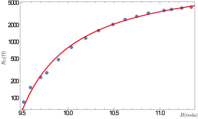
Figure 3: Sheet resistance $R_{\Box}$ of homogeneously-disordered InO_x thin films as a function of perpendicular magnetic field $B$ near the field driven SIT (data extracted from Ref. Steiner et al. (2005)). The fits are to a Kosterlitz-Thouless (KT) law $R_{\Box}=5.02\times 10^{4}e^{-16/\sqrt{B^{2}-9.2^{2}}}$ (solid red curve) and the non-KT law $R_{\Box}=1.53\times 10^{4}e^{-61.2/(B^{2}-8.9^{2})}$ (blue dashed curve). The KT transition is driven by thermal phase fluctuations while the non-KT transition is driven by phase frustration. Both the laws fit the data equally well; however the pre-factor of the exponential, which represents the high-field sheet resistance, is a more reasonable number in the non-KT case since in the actual data, the peak value of resistance is of a comparable order.

.2 Comparison of Kosterlitz-Thouless (KT) and non-KT scaling with experiments

In Fig.3, we show the sheet resistance $R_{\Box}$ vs. magnetic field data near a field-driven SIT in a homogeneously-disordered InO_x thin film from Ref. Steiner et al. (2005), and attempt fits of this data to the Kosterlitz-Thouless (KT) behavior ($R_{\Box}=R_{0}e^{-1/\sqrt{B-B_{KT}}}$) and the non-KT behavior ($R_{\Box}=R_{0}e^{-1/(B-B_{AB})}$) obtained in this Letter. It is difficult to say which of these two laws describes the data better; however, we argue that the non-KT fit might be a bit better on account of a more reasonable value for the high-field resistance $R_{0}.$

References

- Sambandamurthy et al. (2004) G. Sambandamurthy, L. Engel, A. Johansson, and D. Shahar, Physical Review Letters 92, 107005 (2004).
- Steiner et al. (2005) M. A. Steiner, G. Boebinger, and A. Kapitulnik, Physical Review Letters 94, 107008 (2005).
- Shangina and Dolgopolov (2003) E. L. Shangina and V. T. Dolgopolov, Physics-Uspekhi 46, 777 (2003).
- Dubi et al. (2006) Y. Dubi, Y. Meir, and Y. Avishai, Physical Review B 73, 054509 (2006).
- Pokrovsky et al. (2010) V. Pokrovsky, G. Falco, and T. Nattermann, Physical Review Letters 105, 267001 (2010).
- Galitski et al. (2005) V. M. Galitski, G. Refael, M. P. Fisher, and T. Senthil, Physical Review Letters 95, 077002 (2005).
- Lopatin and Vinokur (2007) A. Lopatin and V. Vinokur, Physical Review B 75, 092201 (2007).
- Stewart et al. (2007) M. Stewart, A. Yin, J. Xu, and J. M. Valles, Science 318, 1273 (2007).
- Breznay et al. (2016) N. P. Breznay, M. A. Steiner, S. A. Kivelson, and A. Kapitulnik, Proceedings of the National Academy of Sciences 113, 280 (2016).
- Paalanen et al. (1992) M. Paalanen, A. Hebard, and R. Ruel, Physical Review Letters 69, 1604 (1992).
- Fisher (1990) M. P. Fisher, Physical Review Letters 65, 923 (1990).
- Ioffe and Larkin (1981) L. Ioffe and A. Larkin, (1981).
- Fisher et al. (1989) M. P. Fisher, P. B. Weichman, G. Grinstein, and D. S. Fisher, Physical Review B 40, 546 (1989).
- Ghosal et al. (1998) A. Ghosal, M. Randeria, and N. Trivedi, Physical Review Letters 81, 3940 (1998).
- Sacépé et al. (2008) B. Sacépé, C. Chapelier, T. Baturina, V. Vinokur, M. Baklanov, and M. Sanquer, Physical Review Letters 101, 157006 (2008).
- Chand et al. (2012) M. Chand, G. Saraswat, A. Kamlapure, M. Mondal, S. Kumar, J. Jesudasan, V. Bagwe, L. Benfatto, V. Tripathi, and P. Raychaudhuri, Physical Review B 85, 014508 (2012).
- Chakrabarti and Dasgupta (1988) A. Chakrabarti and C. Dasgupta, Physical Review B 37, 7557 (1988).
- Kim and Stroud (2008) K. Kim and D. Stroud, Physical Review B 78, 174517 (2008).
- Spivak and Zhou (1995) B. Spivak and F. Zhou, Physical Review Letters 74, 2800 (1995).
- Galitski and Larkin (2001) V. Galitski and A. Larkin, Physical Review Letters 87, 087001 (2001).
- Ambegaokar and Baratoff (1963) V. Ambegaokar and A. Baratoff, Physical Review Letters 10, 486 (1963).
- Lifshitz (1968) I. Lifshitz, Soviet Physics JETP 26 (1968).
- Larkin and Vinokur (1995) A. Larkin and V. Vinokur, Physical review letters 75, 4666 (1995).
- Falco et al. (2009) G. Falco, T. Nattermann, and V. L. Pokrovsky, Physical Review B 80, 104515 (2009).
- Altman et al. (2004) E. Altman, Y. Kafri, A. Polkovnikov, and G. Refael, Physical Review Letters 93, 150402 (2004).
- Giamarchi and Schulz (1988) T. Giamarchi and H. Schulz, Physical Review B 37, 325 (1988).
- Teitel and Jayaprakash (1983) S. Teitel and C. Jayaprakash, Physical Review Letters 51, 1999 (1983).
- Van der Zant et al. (1996) H. Van der Zant, W. Elion, L. Geerligs, and J. Mooij, Physical Review B 54, 10081 (1996).
- Carpentier and Le Doussal (2000) D. Carpentier and P. Le Doussal, Nuclear Physics B 588, 565 (2000).
- Carpentier and Le Doussal (1998) D. Carpentier and P. Le Doussal, Physical Review Letters 81, 2558 (1998).
- Biscaras et al. (2013) J. Biscaras, N. Bergeal, S. Hurand, C. Feuillet-Palma, A. Rastogi, R. Budhani, M. Grilli, S. Caprara, and J. Lesueur, Nature Materials 12, 542 (2013).
- Tripathi and Loh (2006) V. Tripathi and Y. Loh, Physical Review Letters 96, 046805 (2006).
- Syzranov et al. (2009) S. Syzranov, K. Efetov, and B. Altshuler, Physical Review Letters 103, 127001 (2009).
- Fistul et al. (2008) M. Fistul, V. Vinokur, and T. Baturina, Physical review letters 100, 086805 (2008).
- Shimshoni et al. (1998) E. Shimshoni, A. Auerbach, and A. Kapitulnik, Physical Review Letters 80, 3352 (1998).
- Petković et al. (2009) A. Petković, V. M. Vinokur, and T. Nattermann, Physical Review B 80, 212504 (2009).
- Oganesyan et al. (2006) V. Oganesyan, D. A. Huse, and S. Sondhi, Physical Review B 73, 094503 (2006).
- Halperin and Nelson (1979) B. Halperin and D. R. Nelson, Journal of Low Temperature Physics 36, 599 (1979).
- Shklovskii (2008) B. Shklovskii, arXiv preprint arXiv:0803.3331 (2008).
- Misra et al. (2013) S. Misra, L. Urban, M. Kim, G. Sambandamurthy, and A. Yazdani, Physical Review Letters 110, 037002 (2013).
- Bramson (1983) M. Bramson, Memoirs of the American Mathematical Society 44, 1 (1983).