On the complexity of minimum-link path problems

Abstract

We revisit the minimum-link path problem: Given a polyhedral domain and two points in it, connect the points by a polygonal path with minimum number of edges. We consider settings where the vertices and/or the edges of the path are restricted to lie on the boundary of the domain, or can be in its interior. Our results include bit complexity bounds, a novel general hardness construction, and a polynomial-time approximation scheme. We fully characterize the situation in 2 dimensions, and provide first results in dimensions 3 and higher for several variants of the problem.

Concretely, our results resolve several open problems. We prove that computing the minimum-link diffuse reflection path, motivated by ray tracing in computer graphics, is NP-hard, even for two-dimensional polygonal domains with holes. This has remained an open problem [1] despite a large body of work on the topic. We also resolve the open problem from [2] mentioned in the handbook [3] (see Chapter 27.5, Open problem 3) and The Open Problems Project [4] (see Problem 22): “What is the complexity of the minimum-link path problem in 3-space?” Our results imply that the problem is NP-hard even on terrains (and hence, due to discreteness of the answer, there is no FPTAS unless P=NP), but admits a PTAS.

1 Introduction

The minimum-link path problem is fundamental in computational geometry [5, 6, 7, 8, 2, 9, 10, 11]. It concerns the following question: given a polyhedral domain $D$ and two points $s$ and $t$ in $D$, what is the polygonal path connecting $s$ to $t$ that lies in $D$ and has as few links as possible?

In this paper, we revisit the problem in a general setting which encompasses several specific variants that have been considered in the literature. First, we nuance and tighten results on the bit complexity involved in optimal minimum-link paths. Second, we present and apply a novel generic NP-hardness construction. Third, we extend a simple polynomial-time approximation scheme.

Concretely, our results resolve several open problems. We prove that computing the minimum-link diffuse reflection path in polygons with holes [1] is NP-hard, and we prove that the minimum-link path problem in 3-space [3] (Chapter 27.5, Open problem 3) is NP-hard (even for terrains). In both cases, there is no FPTAS unless P=NP, but there is a PTAS.

We use terms links and bends for edges and vertices of the path, saving the terms edges and vertices for those of the domain (also historically, minimum-link paths used to be called minimum-bend [12, 13, 14]).

1.1 Problem Statement, Domains and Constraints

Due to their diverse applications, many different variants of minimum-link paths have been considered in the literature. These variants can be categorized by two aspects. Firstly, the domain can take very different forms. We select several common domains, ranging from a simple polygon in 2D to complex scenes in full 3D or even in higher dimensions. Secondly, the links and bends of the solution paths are sometimes constrained to lie on the boundary of the domain, or bends may be restricted to vertices or edges of the domain. We now survey these settings in more detail.

Problem Statement

Let $D$ be a closed connected $d$-dimensional polyhedral domain. For $0\leq a\leq d$ we denote by $D|^{a}$ the $a$-skeleton of $D$; that is, its $a$-dimensional subcomplex. For instance, $D|^{d-1}$ is the boundary of $D$; $D|^{0}$ is the set of vertices of $D$. Note that $D|^{a}$ is not necessarily connected.

Definition 1.

We define $\textsf{MinLinkPath}_{a,b}(D,s,t)$, for $0\leq a\leq b\leq d$ and $1\leq b$, to be the problem of finding a minimum-link polygonal path in $D$ between two given points $s$ and $t$, where the bends of the solution (and $s$ and $t$) are restricted to lie in $D|^{a}$ and the links of the solution are restricted to lie in $D|^{b}$.

Fig. 1 illustrates several instances of the problem in different domains.

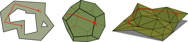
Figure 1: Left: MinLinkPath_2,2 in a polygon with holes. Middle: MinLinkPath_1,2 on a polyhedron. Right: MinLinkPath_0,3 on a polyhedral terrain.

Domains

We recap the various settings that have been singled out for studies in computational geometry. We remark that we will not survey the rich field of path planning in rectilinear, or more generally, $C$-oriented worlds [15]; all our paths will be assumed to be unrestricted in terms of orientations of their links.

One classical distinction between working setups in 2D is simple polygons vs. polygonal domains. The former are a special case of the latter: simple polygons are domains without holes. Many problems admit more efficient solutions in simple polygons—loosely speaking, the golden standard is running time of $O(n)$ for simple polygons and of $O(n\log n)$ for polygonal domains of complexity $n$. This is the case, e.g., for the shortest path problem [16, 17]. For minimum-link paths, $O(n)$-time algorithms are known for simple polygons [5, 6, 7], but for polygonal domains with holes the fastest known algorithm runs in nearly quadratic time [2], which may be close to optimal due to 3SUM-hardness of the problem [9]. Even more striking is the difference in the watchman route problem (find a shortest path to see all of the domain), which combines path planning with visibility: in simple polygons the optimal route can be found in polynomial time [18, 19] while for domains with holes the problem cannot be approximated to within a logarithmic factor unless P=NP [20]. Finding minimum-link watchman route is NP-hard even for simple polygons [21].

In 3D, a terrain is a polyhedral surface (often restricted to a bounded region in the $xy$-projection) that is intersected only once by any vertical line. Terrains are traditionally studied in GIS applications and are ubiquitous in computational geometry [22, 23]. Minimum-link paths are closely related to visibility problems, which have been studied extensively on terrains [24, 25, 26, 27, 28, 29]. One step up from terrains, we may consider simple polyhedra (surfaces of genus $0$), or full 3D scenes. Visibility has been studied in full 3D as well [30, 31, 32]. To our knowledge, minimum-link paths in higher dimensions have not been studied before (with the exception of [33] that considered rectilinear paths).

Constraints

In path planning on polyhedral surfaces or terrains, it is standard to restrict paths to the terrain. Minimum-link paths, on the other hand, have various geographic applications, ranging from feature simplification [11] to visibility in terrains [24]. In some of these applications, paths are allowed to live in free space, while bends are still restricted to the terrain. In the GIS literature, out of simplicity and/or efficiency concerns, it is common to constrain bends even further to vertices of the domain (or, even more severely, the terrain itself may restrict vertices to grid points, as in the popular digital elevation map (DEM) model).

In a vanilla min-link path problem the location of vertices (bends) of the path are unconstrained, i.e., they can occur anywhere in the free space. In the diffuse reflection model [1, 34, 35, 36, 37, 10] the bends are restricted to occur on the boundary of the domain. Studying this kind of paths is motivated by ray tracing in realistic rendering of 3D scenes in graphics, as light sources that can reach a pixel with fewer reflections make higher contributions to intensity of the pixel [38, 22]. Despite the 3D graphics motivation, all work on diffuse reflection has been confined to 2D polygonal domains, where the path bends are restricted to edges of the domain.

1.2 Representation and Computation

In computational geometry, the standard model of computation is the Real RAM, which represents data as an infinite sequence of storage cells which can store any real number or integer. The model supports standard operations (such as addition, multiplication, or taking square-roots) in constant time. The Real RAM is preferred for its elegance, but may not always be the best representation of physical computers. For example, the floor function is often allowed, which can be used to truncate a real number to the nearest integer, but points at a flaw in the model: if we were allowed to use it arbitrarily, the Real RAM could solve PSPACE-complete problems in polynomial time [39]. In contrast, the word RAM stores a sequence of $w$-bit words, where $w\geq\log n$ (and $n$ is the problem size). Data can be accessed arbitrarily, and standard operations, such as Boolean operations (and, xor, shl, $\ldots$), addition, or multiplication take constant time. There are many variants of the word RAM, depending on precisely which instructions are supported in constant time. The general consensus seems to be that any function in $\text{AC}^{0}$ is acceptable. However, it is always preferable to rely on a set of operations as small, and as non-exotic, as possible. Note that multiplication is not in $\text{AC}^{0}$ [40]. Nevertheless, it is usually included in the word RAM instruction set [41]. The word RAM is much closer to reality, but complicates the analysis of geometric problems.

In many cases, the difference is unimportant, as the real numbers involved in solving geometric problems are in fact algebraic numbers of low degree in a bounded domain, which can be described exactly with constantly many words. Path planning is notoriously different in this respect. Indeed, in the Real RAM both the Euclidean shortest paths and the minimum-link paths in 2D can be found in optimal times. On the contrary, much less is known about the complexity of the problems in other models. For $L_{2}$-shortest paths the issue is that their length is represented by the sum of square roots and it is not known whether comparing the sum to a number can be done efficiently (if yes, one may hope that the difference between the models vanishes). Slightly more is known about minimum-link paths, for which the models are provably different: Snoeyink and Kahan [8] observed that the region of points reachable by $k$-link paths may have vertices needing $\Omega(k\log n)$ bits to describe. One of the results in this paper is the matching upper bound on the bit complexity of min-link paths.

Relatedly, when studying the computational complexity of geometric problems, it is often not trivial to show a problem is in NP. Even if a potential solution can be verified in polynomial time, if such a solution requires real numbers that cannot be described succinctly, the set of solutions to try may be too large. Recently, there has been some interest in computational geometry in showing problems are in NP [42] (see also [43]).

A common practical approach to avoiding bit complexity issues is to approximate the problem by restricting solutions to use only vertices of the input. In minimum-link paths, this corresponds to MinLinkPath_0,b. Although such paths can be computed efficiently, a simple example (Appendix 8) shows that the number of links in such a setting may be a linear factor higher than when considering geometric versions.

1.3 Results

We give hardness results and approximation algorithms for various versions of the min-link path problem. Specifically,

• In Section 2 we show a general lower bound on the bit complexity of min-link paths of $\Omega(n\log n)$ bits for some coordinates. (This was previously claimed, but not proven, by Snoeyink and Kahan [8].) We show that the bound is tight in 2D and we argue that this implies that MinLinkPath_a,2 is in NP. In Section 5, we argue that in 3D the boundary of the $k$-illuminated region can consist of $k$-th order algebraic curves, potentially leading to exponential bit complexity.

• In Section 3.1 we present a blueprint for showing NP-hardness of minimum link problems. We apply it to prove NP-hardness of the diffuse reflection path problem (MinLinkPath_1,2) in 2D polygonal domains with holes in Section 3.2. In Section 6, we use the same blueprint to prove that all non-trivial versions, defined above, of min-link problems in 3D are weakly NP-hard. We also note that the min-link problems have no FPTAS and no additive approximation (unless P=NP).

• In Section 4 we extend the 2-approximation algorithm from [3, Ch. 27.5], based on computing weak visibility between sets of potential locations of the path’s bends, to provide a simple PTAS for MinLinkPath_2,2, which we also adapt to MinLinkPath_1,2. In Section 7 we give simple constant-factor approximation algorithms for higher-dimensional minimum-link path versions, which can then be used in the same way to show that all versions admit PTASes.

• In Section 7.3 we focus on MinLinkPath_2,3 (diffuse reflection in 3D) on terrains—the version that is most important in practice. We give a 2-approximation algorithm that runs faster than the generic algorithm from [3, Ch. 27.5]. We also present an $O(n^{4})$-size data structure encoding visibility between points on a terrain and argue that the size of the structure is asymptotically optimal.

Our results are charted and compared to existing results in Table 1.

MinLinkPatha,b	$b=1$	$b=2$	$b=3$
$a=0$	$O(n)$	$O(n^{2})$	$O(n^{2})$
$a=1$	$O(n)$	Simple Polygon: $O(n^{9})$[10] Full 2D: NP-hard$\star$ PTAS$\star$	NP-hard$\star$ (even in terrains) PTAS$\star$
$a=2$	N/A	Simple Polygon: $O(n)$[5] Full 2D: $O(n^{2}\alpha(n)\log^{2}{n})$[2] PTAS$\star$	NP-hard$\star$ (even in terrains) PTAS$\star$
$a=3$	N/A	N/A	Terrains: $O(1)$ Full 3D: NP-hard$\star$ PTAS$\star$

Table 1: Computational complexity of MinLinkPath_a,b for $a\leq b\leq 3$. Results with citations are known, results marked with $\star$ are from this paper. Results without marks are trivial.

2 Algebraic Complexity in $\mathbb{R}^{2}$

2.1 Lower bound on the Bit complexity

Snoeyink and Kahan [8] claim to “give a simple instance in which representing path vertices with rational coordinates requires $\Theta(n^{2}\log n)$ bits”. In fact, they show that the boundary of the region reachable from $s$ (a point with integer coordinates specified with $O(\log n)$ bits) with $k$ links may have vertices whose coordinates have bit complexity $k\log n$. Note however, that this does not directly imply that a minimum-link path from $s$ to another point $t$ with low-complexity (integer) coordinates must necessarily have such high-complexity bends (i.e., if $t$ itself is not a high-complexity vertex of a $k$-reachable region, one potentially could hope to avoid also placing the internal vertices of a min-link path to $t$ on such high-complexity points). Below we present a construction where the intermediate vertices must actually use $\Omega(k\log n)$ bits to be described, even if $s$ and $t$ can be specified using only $\log n$ bits each. We first prove this for the MinLinkPath_1,2 variant of the problem, and then extend our results to paths that may bend anywhere within the polygon, i.e. MinLinkPath_2,2.

Lemma 1.

There exists a simple polygon $P$, and points $s$ and $t$ in $P$ such that: (i) all the coordinates of the vertices of $P$ and of $s$ and $t$ can be represented using $O(\log n)$ bits, and (ii) any $s$-$t$ min-link path that bends only on the edges of $P$ has vertices whose coordinates require $\Omega(k\log n)$ bits, where $k$ is the length of a min-link path between $s$ and $t$.

Proof.

We will refer to numbers with $O(\log n)$ bits as low-complexity.

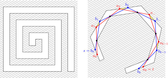
Figure 2: (a) A spiral, as used in the construction by Kahan and Snoeyink. It uses integer coordinates with $O(\log n)$ bits. (b) The general idea.

The general idea in our construction is as follows. We start with a low-complexity point $s^{\prime}=b_{0}$ on an edge $e_{0}$ of the polygon. We then consider the furthest point $b_{i+1}$ on the boundary of $P$ that is reachable from $b_{i}$. More specifically, we require that any point on the boundary of $P$ between $s^{\prime}$ and $b_{i}$ is reachable by a path of at most $i$ links. We will obtain $b_{i+1}$ by projecting $b_{i}$ through a vertex $c_{i}$. Each such a step will increase the required number of bits for $b_{i+1}$ by $\Theta(\log n)$. Eventually, this yields a point $b_{k}$ on edge $e_{k}$. Let $t^{\prime}$ be the $k$-reachable point on $e_{k}$ closest to $b_{k}$ that has low complexity. Since all points along the boundary from $s^{\prime}$ to $b_{k}$ are reachable, and the vertices of $P$ have low complexity, such a point is guaranteed to exist. We set $a_{k}=t^{\prime}$ and project $a_{i}$ through $c_{i-1}$ to $a_{i-1}$ to give us the furthest point (from $t^{\prime}$) reachable by $k-i$ links. See Fig. 2 for an illustration.

The points in the interval $I_{i}=[a_{i},b_{i}]$, with $1\leq i<k$, are reachable from $s^{\prime}$ by exactly $i$ links, and reachable from $t^{\prime}$ by exactly $k-i$ links. So, to get from $s^{\prime}$ to $t^{\prime}$ with $k$ links, we need to choose the $i^{\textrm{th}}$ bend of the path to be within the interval $[a_{i},b_{i}]$. By construction, the intervals for $i$ close to one or close to $k$ must contain low-complexity points. We now argue that we can build the construction in such a way that $I_{k/2}$ contains no low-complexity points.

Observe that, if an interval contains no points that can be described with fewer than $m$ bits, its length can be at most $2^{-m}$. So, we have to show that $I_{k/2}$ has length at most $2^{-k\log n}$.

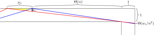
Figure 3: The interval $I_{i}$ of length $w_{i}$ produces an interval $I_{i+1}$ of length at most $w_{i+1}=h_{i}/\Theta(n)=\Theta(w_{i}/n^{2})$, where $h_{i}=w_{i}/(w_{i}+\Theta(n))$. When the $i^{\mathrm{th}}$ link can be anywhere in region $R_{i}$ (shown in yellow), it follows that $R_{i}$ has height at most $h_{i}$, and width at most $w_{i}$.

By construction, the interval $I_{k}$ has length at most one. Similarly, the length of $I_{0}$ can be chosen to be at most one (if it is larger, we can adjust $s^{\prime}=b_{0}$ to be the closest integer point to $a_{0}$). Now observe that that in every step, we can reduce the length $w_{i}$ of the interval $I_{i}$ by a factor $\Theta(n^{2})$, using a construction like in Fig. 3. Our overall construction is then shown in Fig. 4.

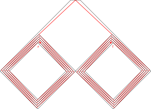
Figure 4: An overview of our polygon $P$ and the minimum-link path that has high-complexity coordinates.

It follows that $I_{k/2}$ cannot contain two low-complexity points that are close to each other. Note however, that it may still contain one such a point. However, it is easy to see that there is a sub-interval $J_{k/2}=[\ell_{k/2},r_{k/2}]\subseteq I_{k/2}$ of length $w_{k/2}/2$ that contains no points with fewer than $k\log n$ bits. By choosing $J_{k/2}$ we have restricted the interval that must contain the $(k/2)^{\mathrm{th}}$ bend. This also restricts the possible positions for the $i^{\mathrm{th}}$ bend to an interval $J_{i}\subseteq I_{i}$. We find these intervals by projecting $\ell_{k/2}$ and $r_{k/2}$ through the vertices of $P$. Note that $s^{\prime}$ and $t^{\prime}$ may not be contained in $J_{0}$ and $J_{k}$, respectively, so we pick a new start point $s\in J_{0}$ and en point $t\in J_{k}$ as follows. Let $m_{k/2}$ be the mid point of $J_{k/2}$ and project $m_{i}$ through the vertices of $P$. Now choose $s$ to be a low-complexity point in the interval $[m_{0},r_{0}]$, and $t$ to be a low-complexity point in the interval $[\ell_{k},m_{k}]$. Observe that $[m_{0},r_{0}]$ and $[\ell_{k},m_{k}]$ have length $\Theta(1)$—as $[\ell_{k/2},m_{k/2}]$ and $[m,_{k/2},r_{k/2}]$ have length $w_{k/2}/4$—and thus contain low complexity points. Furthermore, observe that $t$ is indeed reachable from $s$ by a path with $k-1$ bends (and thus $k$ links), all of which much lie in the intervals $J_{i}$, $1\leq i<k$. For example using the path that uses all points $m_{i}$. Thus, we have that $t$ is reachable from $s$ by a minimum-link path of $k$ links, and we need $\Omega(k\log n)$ bits to describe the coordinates of the vertices in such a path. ∎

Lemma 2.

There exists a simple polygon $P$, and points $s$ and $t$ in $P$ such that: (i) all the coordinates of the vertices of $P$ and of $s$ and $t$ can be represented using $O(\log n)$ bits, and (ii) any $s$-$t$ min-link path has vertices whose coordinates require $\Omega(k\log n)$ bits, where $k$ is the length of a min-link path between $s$ and $t$.

Proof.

We extend the construction from Lemma 1 to the case in which the bends may also lie in the interior of $P$. Let $B_{i}$ denote the region in $P$ that is reachable from $s^{\prime}$ by exactly $i$ links, let $A_{i}$ the region reachable from $t^{\prime}$ by exactly $k-i$ links, and let $R_{i}=B_{i}\cap A_{i}$. To get from $s^{\prime}$ to $t^{\prime}$ with $k$ links, the $i^{\textrm{th}}$ bend has to lie in $R_{i}$. Now observe that this region is triangular, and incident to the interval $I_{i}$ (see e.g. Fig. 3 for an illustration). This region $R_{i}$ has width at most $w_{i}$ and height at most $h_{i}=w_{i}/(w_{i}+\Theta(n))$. Therefore, we can again argue that $R_{k/2}$ is small, and thus contains at most one low-complexity point $p$. We then again choose a region $R^{\prime}_{k/2}\subseteq R_{k/2}$ of diameter $w_{k/2}/2$ that avoids point $p$. The remainder of the argument is analogous to the one before; we can pick points $s$ and $t$ in the restricted regions $R^{\prime}_{0}$ and $R^{\prime}_{k}$ that are reachable by a minimum-link path of $k-1$ bends, all of which have to lie in the regions $R^{\prime}_{i}$. It follows that we again need $\Omega(k\log n)$ bits to describe the coordinates of the vertices in such a path. ∎

2.2 Upper bound on the Bit complexity

We now show that the bound of Snoeyink and Kahan [8] on the complexity of $k$-link reachable regions is tight: representing the regions $\mathcal{R}$ as polygons with rational coordinates requires $O(n^{2}\log n)$ for any polygon $P$, assuming that representation of the coordinates of any vertex of $P$ requires at most $c_{0}\log n$ bits for some constant $c_{0}$. Thus, we have a matching lower and upper bound on the bit complexity of a minimum-link path in $\mathbb{R}^{2}$.

Consider a simple polygon $P$ with $n$ vertices, and a point $s\in P$. Analogous to [8], define a sequence of regions $\mathcal{R}=\{R_{1},R_{2},R_{3},\dots\}$, where $R_{1}$ is a set of all points in $P$ that see $s$, and $R_{i+1}$ is a region of points in $P$ that see some point in $R_{i}$ for $i\geq 1$. In other words, region $R_{i+1}$ consists of all the points of $P$ that are illuminated by region $R_{i}$.

Construction of region $R_{i+1}$.

If $P$ is a simple polygon, then $R_{i+1}$ is also a simple polygon, consisting of $O(n)$ vertices. We will bound the bit complexity of a single vertex of $R_{i+1}$. The vertices of such a region are either

• original vertices of $P$,

• intersection points of $P$’s boundary with lines going through reflex vertices of $P$, or

• intersection points of $P$’s boundary with rays emanating from the vertices of $R_{i}$ and going through reflex vertices of $P$.

Only the last type of vertices can lead to an increase in bit complexity. Each of these vertices is defined as an intersection point of two lines: one of the lines passes through two vertices of $P$, say $a=(x_{a},y_{a})$ and $b=(x_{b},y_{b})$, and, therefore, has a $O(\log n)$ bit representation. The other line passes through one vertex of $P$, say $c=(x_{c},y_{c})$, with coordinates of $O(\log n)$ bit complexity, and one vertex of region $R_{i}$, say $d=(x_{d},y_{d})$, with coordinates of potentially higher complexity. The coordinates of the intersection can then be calculated by the following formula:

$$\begin{pmatrix}x^{*}\\ y^{*}\end{pmatrix}=\begin{pmatrix}\dfrac{(x_{b}y_{a}-x_{a}y_{b}+x_{a}y_{c}-x_{b}y_{c})x_{d}+(x_{b}x_{c}-x_{a}x_{c})y_{d}+x_{a}y_{b}x_{c}-y_{a}x_{b}x_{c}}{(y_{a}-y_{b})x_{d}-(x_{a}-x_{b})y_{d}+x_{a}y_{c}-y_{a}x_{c}-x_{b}y_{c}+y_{b}x_{c}}\\[12.0pt] \dfrac{(y_{a}y_{c}-y_{b}y_{c})x_{d}+(x_{b}y_{a}-x_{c}y_{a}-x_{a}y_{b}+x_{c}y_{b})y_{d}+x_{a}y_{b}y_{c}-y_{a}x_{b}y_{c}}{(y_{a}-y_{b})x_{d}-(x_{a}-x_{b})y_{d}+x_{a}y_{c}-y_{a}x_{c}-x_{b}y_{c}+y_{b}x_{c}}\end{pmatrix}=\begin{pmatrix}\dfrac{A^{\prime}_{1}x_{d}+B^{\prime}_{1}y_{d}+C^{\prime}_{1}}{E^{\prime}x_{d}+F^{\prime}y_{d}+G^{\prime}}\\[12.0pt] \dfrac{A^{\prime}_{2}x_{d}+B^{\prime}_{2}y_{d}+C^{\prime}_{2}}{E^{\prime}x_{d}+F^{\prime}y_{d}+G^{\prime}}\end{pmatrix}\,.$$ (1)

Point $d$ lies on the boundary of $P$. Denote the end points of the side it belongs to as $u$ and $v$. Then the following relation between the coordinates of $d$ holds:

$$y_{d}=\frac{(y_{u}-y_{v})x_{d}+x_{u}y_{v}-y_{u}x_{v}}{x_{u}-x_{v}}\,.$$

Thus, Equation 1 can be rewritten as:

$$\begin{pmatrix}x^{*}\\ y^{*}\end{pmatrix}=\begin{pmatrix}\dfrac{A_{1}x_{d}+B_{1}}{Cx_{d}+D}\\[12.0pt] \dfrac{A_{2}x_{d}+B_{2}}{Cx_{d}+D}\end{pmatrix}\,,$$ (2)

where each of $A_{1}$, $A_{2}$, $B_{1}$, $B_{2}$, $C$, and $D$ has bit complexity not greater than $c\log n$ for some constant $c$ (here, it is enough to choose $c=4c_{0}$). Let $x_{d}$ be represented as a rational number $\raise 2.15277pt\hbox{$p$}\kern-1.00006pt/\kern-1.49994pt\lower 1.07639pt\hbox{$q$}$, where $p$ and $q$ are mutually prime integers. Then the number of bits required to represent $x_{d}$ is $sp(x_{d})=\lceil\log(p+1)\rceil+\lceil\log(q+1)\rceil\geq\log(p+1)+\log(q+1)\geq 2\log(p+q)$, the last inequality holds for all $p\geq 1$ and $q\geq 1$. Therefore, the number of bits required to represent $x^{*}$ is

$$\begin{split}sp(x^{*})&=\lceil\log(A_{1}p+B_{1}q+1)\rceil+\lceil\log(Cp+Dq+1)\rceil\leq 2\lceil\log(E(p+q)+1)\rceil\leq\\ &\leq 2\log E+2\log(p+q)+2\leq 2+2c\log n+sp(x_{d})\,,\end{split}$$

where $E=\max\{A_{1},B_{1},C,D\}$. Analogously for $y^{*}$, $sp(y^{*})\leq 2+2c\log n+sp(x_{d})$. Therefore, at every step, the bit complexity of the coordinates grows no more than by an additive value $2+2c\log n$. After $n$ steps, the bit-complexity of the regions’ vertices is $O(n\log n)$.

Theorem 3.

Representing the regions $\mathcal{R}$ as polygons with rational coordinates requires $O(n^{2}\log n)$ bits.

Corollary 4.

If there exists a solution with $k$ links, there also exists one in which the coordinates of the bends use at most $O(k\log n)$ bits.

Theorem 5.

MinLinkPath_a,2 is in NP.

Proof.

We need to show that a candidate solution can be verified in polynomial time. A potential solution needs at most $n$ links. By Corollary 4, we only need to verify candidate solutions that consist of bends with $O(n\log n)$-bit coordinates. Given such a candidate, we need to verify pairwise visibility between at most $n$ pairs of points with $O(n\log n)$-bit coordinates, which can be done in polynomial time. ∎

3 Computational Complexity in $\mathbb{R}^{2}$

In this section we show that MinLinkPath_1,2 is NP-hard. To this end, we first provide a blueprint for our reduction in Section 3.1. In Section 3.2 we then show how to “instantiate” this blueprint for MinLinkPath_1,2 in a polygon with holes.

3.1 A Blueprint for Hardness Reductions

We reduce from the 2-Partition problem: Given a set of integers $A=\{a_{1},\dots,a_{m}\}$, find a subset $S\subseteq A$ whose sum is equal to half the sum of all numbers. The main idea behind all the hardness reductions is as follows. Consider a 2D construction in Fig. 5 (left). Let point $s$ have coordinates $(0,0)$, and $t$ (not in the figure) have coordinates $(\sum a_{i}/2,4m-2)$. For now, in this construction, we will consider only paths from $s$ to $t$ that are allowed to bend on horizontal lines with even $y$-coordinates. Moreover, we will count an intersection with each such horizontal line as a bend. We will place fences along the lines with odd $y$-coordinates in such a way that an $s$-$t$ path with $2m-1$ links exists (that bends only on horizontal lines with even $y$-coordinates) if and only if there is a solution to the 2-Partition instance.

Call the set of horizontal lines $\ell_{0}:y=0$, $\ell_{i}:y=4i-2$ for $1\leq i\leq m$ important (dashed lines in Fig. 5), and the set of horizontal lines $\ell^{\prime}_{i}:y=4i-4$ for $2\leq i\leq m$ intermediate (dash-dotted lines in Fig. 5). Each important line $\ell_{i}$ will “encode” the running sums of all subsets of the first $i$ integers $A_{i}=\{a_{1},\dots,a_{i}\}$. That is, the set of points on $\ell_{i}$ that are reachable from $s$ with $2i-1$ links will have coordinates $(\sum_{a_{j}\in S_{i}}a_{j},4i-2)$ for all possible subsets $S_{i}\subseteq A_{i}$.

Call the set of horizontal lines $f_{1}:y=1$, $f_{i}:y=4i-5$ for $2\leq i\leq m$ multiplying, and the set of horizontal lines $f^{\prime}_{i}:y=4i-3$ for $2\leq i\leq m$ reversing. Each multiplying line $f_{i}$ contains a fence with two $0$-width slits that we call $0$-slit and $a_{i}$-slit. The $0$-slit with $x$-coordinate $0$ corresponds to not including integer $a_{i}$ into subset $S_{i}$, and the $a_{i}$-slit with $x$-coordinate $\sum_{1}^{i}{a_{j}}-a_{i}/2$ corresponds to including $a_{i}$ into $S_{i}$. Each reversing line $f^{\prime}_{i}$ contains a fence with two $0$-width slits (reversing $0$-slit and reversing $a_{i}$-slit) with $x$-coordinates $0$ and $\sum_{1}^{i}{a_{j}}$ that “put in place” the next bends of potential min-link paths, i.e., into points on $\ell_{i}$ with $x$-coordinates equal to running sums of $S_{i}$. We add a vertical fence of length $1$ between lines $\ell^{\prime}_{i}$ and $f^{\prime}_{i}$ at $x$-coordinate $\sum_{1}^{i}{a_{j}}/2$ to prevent the min-link paths that went through the multiplying $0$-slit from going through the reversing $a_{i}$-slit, and vice versa.

As an example, consider (important) line $\ell_{2}$ in Fig. 5. The four points on $\ell_{2}$ that are reachable from $s$ with $3$ links have $x$-coordinates $\{0,a_{1},a_{2},a_{1}+a_{2}\}$. The points on line $\ell^{\prime}_{3}$ that are reachable from $s$ with a path (with $4$ links) that goes through the $0$-slit on line $f_{3}$ have $x$-coordinates $\{0,-a_{1},-a_{2},-(a_{1}+a_{2})\}$, and the points on $\ell^{\prime}_{3}$ that are reachable from $s$ through the $a_{3}$-slit have $x$-coordinates $\{a_{1}\!+\!a_{2}\!+\!a_{3},2a_{1}\!+\!a_{2}\!+\!a_{3},a_{1}\!+\!2a_{2}\!+\!a_{3},2a_{1}\!+\!2a_{2}+a_{3}\}$. The reversing $0$-slit on line $f^{\prime}_{3}$ places the first four points on $\ell_{3}$ into $x$-coordinates $\{0,a_{1},a_{2},a_{1}+a_{2}\}$, and the reversing $a_{3}$-slit places the second four points on $\ell_{3}$ into $x$-coordinates $\{a_{3},a_{1}+a_{3},a_{2}+a_{3},a_{1}+a_{2}+a_{3}\}$.

In general, consider some point $p$ on line $\ell_{i-1}$ that is reachable from $s$ with $2i-3$ links. The two points on $\ell^{\prime}_{i}$ that can be reached from $p$ with one link have $x$-coordinates $-p_{x}$ and $2\sum_{1}^{i}{a_{j}}-a_{i}-p_{x}$, where $p_{x}$ is the $x$-coordinate of $p$. Consequently, the two points on $\ell_{i}$ that can be reached from $p$ with two links have $x$-coordinates $p_{x}$ and $p_{x}+a_{i}$. Therefore, for every line $\ell_{i}$, the set of points on it that are reachable from $s$ with a min-link path have $x$-coordinates equal to $\sum_{a_{j}\in S_{i}}a_{j}$ for all possible subsets $S_{i}\subseteq A_{i}$. Consider line $\ell_{m}$ and the destination point $t$ on it. There exists a $s$-$t$ path with $2m-1$ links if and only if the $x$-coordinate of $t$ is equal to $\sum_{a_{j}\in S}a_{j}$ for some $S\subseteq A$. The complexity of the construction is polynomial in the size of the 2-Partition instance. Therefore, finding a min-link path from $s$ to $t$ in our 2D construction is $NP$-hard.

Figure 5: The first few lines of a 2D construction depicting the general idea behind the hardness proofs: important lines $\ell_{0}$–$\ell_{3}$, intermediate lines $\ell^{\prime}_{1}$–$\ell^{\prime}_{3}$, multiplying lines $f_{1}$–$f_{3}$, and reversing lines $f^{\prime}_{1}$–$f^{\prime}_{3}$. The slits in the fences on multiplying and reversing lines are placed in such a way that the locations on $\ell_{i}$ that are reachable from $s$ with $2i-1$ links correspond to sums formed by all possible subsets of $\{a_{1},\dots,a_{i}\}$.

3.2 Hardness of MinLinkPath_1,2

We can turn our construction from Section 3.1 into a “zigzag” polygon (Fig. 6); the fences are turned into obstacles within the corresponding corridors, and slits remain slits—the only free space through which it is possible to go with one link between the polygon edges that correspond to consecutive lines $\ell^{\prime}_{i}$ and $\ell_{i}$ (or $\ell_{i-1}$ and $\ell^{\prime}_{i}$). This retains the crucial property of 2D construction: locations reachable with fewest links on the edges of the polygon correspond to sums of numbers in the subsets of $A$. We conclude:

Theorem 6.

MinLinkPath_1,2 in a 2D polygonal domain with holes is NP-hard.

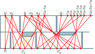
Figure 6: There exists an $s$-$t$ diffuse reflection path with $2m-1$ links iff 2-Partition instance is feasible.

Overall our reduction bears resemblance to the classical path encoding scheme [44] used to prove hardness of 3D shortest path and other path planning problems, as we also repeatedly double the number of path homotopy types; however, since we reduce from 2-Partition (and not from 3SAT, as is common with path encoding), our proof(s) are much less involved than a typical path-encoding one.

No FPTAS.

Obviously, problems with a discrete answer (in which a second-best solution is separated by at least 1 from the optimum) have no FPTAS. For example, in the reduction in Theorem 6, if the instance of 2-Partition is feasible, the optimal path has $2m-1$ links; otherwise it has $2m$ links. Suppose there exists an algorithm, which, for any $\varepsilon>0$ finds a $(1+\varepsilon)$-approximate solution in time polynomial in $1/\varepsilon$. Take $\varepsilon=\frac{1}{2m-1}$; note that 1/$\varepsilon$ is polynomial, and hence the FPTAS with this $\varepsilon$ will complete in polynomial time. For an infeasible instance of 2-Partition the FPTAS would output a path with at least $2m$ links, while for a feasible instance it will output a path with at most $(1+\varepsilon)(2m-1)=2m-1/2$ links. There is only one such length possible; a path with exactly $\mathsf{opt}=2m-1$ links. Hence, the FPTAS would be able to differentiate, in polynomial time, between feasible and infeasible instances of 2-Partition.

No additive approximation.

We can slightly amplify the hardness results, showing that for any constant $K$ it is not possible to find an additive-$K$ approximation for our problems: Concatenate $K$ instances of the construction from the hardness proof, aligning $s$ in the instance $k+1$ with $t$ from the instance $k$. Then there is a path with $K(2m-1)$ links through the combined instance if the 2-Partition is feasible; otherwise $K(2m-1)+K-1$ links are necessary, Thus an algorithm, able to differentiate between instances in which the solution has $K(2m-1)$ links and those with $K(2m-1)+K-1$ links in $\textrm{poly}(mK)=\textrm{poly}(m)$ time, would also be able to solve 2-Partition in the same time.

4 Algorithmic Results in $\mathbb{R}^{2}$

4.1 Constant-factor Approximation

MinLinkPath_2,2 can be solved exactly [2]. For MinLinkPath_1,2, [1] gives a $3$-approximation.

4.2 PTAS

We describe a $(1+\varepsilon)$-approximation scheme for MinLinkPath_1,2, based on building a graph of edges of $D$ that are $k$-link weakly visible.

Consider the set $F$ of all edges of $D$ (that is, $\bigcup F=D|^{1}$). To avoid confusion between edges of $D$ and edges of the graph we will build, we will call elements of $F$ features (this will also allow us to extend the ideas to higher dimensions later). Two features $f,f^{\prime}\in F$ are weakly visible if there exist mutually visible points $p\in f,p^{\prime}\in f^{\prime}$; more generally, we say $f,f^{\prime}$ are $k$-link weakly visible if there exists a $k$-link path from $p$ to $p^{\prime}$ (with the links restricted to $D|^{1}$).

For any constant $k\geq 1$, we construct a graph $G^{k}=(F,E_{k})$, where $E_{k}$ is the set of pairs of $k$-link weakly visible features. Let $\pi^{k}=\{f_{0},f_{1},\dots,f_{\ell}\}$, with $f_{0}\ni s$ and $f_{\ell}\ni t$ be a shortest path in $G$ from the feature containing $s$ to the feature containing $t$; $\ell$ is the number of links of $\pi$. We describe how to transform $\pi^{k}$ into a solution to the MinLinkPath_1,2 problem. Embed edges of $\pi$ into $D$ as $k$-link paths. This does not necessarily connect $s$ to $t$ since it could be that, inside a feature $f_{i}$, the endpoint of the edge $f_{i-1}f_{i}$ does not coincide with endpoint of the edge $f_{i}f_{i+1}$; to create a connected path, we observe that the two endpoints can always be connected by two extra links via some feature that is mutually visible from both points (or a single extra link within $f_{i}$ if we allow links to coincide within the boundary of $D$).

Lemma 7.

The number of links in $\pi^{k}_{*}$ is at most $(1+1/k)\mathsf{opt}$.

Proof.

Split $\mathsf{opt}$ into pieces of $k$ links each (the last piece may have fewer than $k$ links); the algorithm will find $k$-link subpaths between endpoints of the pieces. In details, suppose that $\mathsf{opt}=mk+r$ where $m,r$ are the quotient and the remainder from division of $\mathsf{opt}$ by $k$; let $s=v_{0},v_{1},\dots,v_{\mathsf{opt}}=t$ be the vertices (bends) of $\mathsf{opt}$, and let $f_{i}$ be the feature to which the $ik$-th bend $v_{ik}$ belongs. Since the link distance between $v_{(i-1)k}$ and $v_{ik}$ is $k$, our algorithm will find a $k$-link subpath from $f_{i-1}$ to $f_{i}$, as well as an $r$-link subpath from $f_{m}$ to $t$. The total number of links in the approximate path is thus at most $mk+m+r\leq(1+1/k)(mk+r)=(1+1/k)\mathsf{opt}$ (if $r=0$, our algorithm will find path with at most $mk+m-1<(1+1/k)mk=(1+1/k)\mathsf{opt}$ links; if $r>0$, our algorithm will find path with at most $mk+r+m\leq(1+1/k)(mk+r)=(1+1/k)\mathsf{opt}$ links). ∎

We now argue that the weak $k$-link visibility between features can be determined in polynomial time using the staged illumination: starting from each feature $f$, find the set $W(f)$ of points on other features weakly visible from $f$, then find the set weakly visible from $W^{2}(f)=W(W(f))$, repeat $k$ times to obtain the set $W^{k}(f)$ reachable from $f$ with $k$ links; feature $f^{\prime}$ can be reached from $f$ in $k$ links iff $W^{k}(f)\cap f^{\prime}\neq\varnothing$. For constant $k$, building $W^{k}(f)$ takes time polynomial in $n$, although possibly exponential in $k$ (in fact, for diffuse reflection explicit bounds on the complexity of $W^{k}(f)$ were obtained [36, 37, 10]). This can be seen by induction: Partition the set $W^{i-1}(f)$ into the polynomial number of constant-complexity pieces. For each piece $p$, each element $e$ of the boundary of the domain and each feature $f^{\prime}$ compute the part of $f^{\prime}$ shadowed by $e$ from the light sources on $p$—this can be done in constant time analogously to determining weak visibility between two features above (by considering the part of $p\times f^{\prime}$ carved out by the occluder $e$). The part of $f^{\prime}$ weakly seen from $W^{i-1}(f)$ is the union, over all parts $p$, of the complements of the sets occluded by all elements $e$; since there is a polynomial number of parts, elements and features, it follows that $W^{i}(f)$ can be constructed in polynomial time.

Theorem 8.

For a constant $k$ the path $\pi^{k}_{*}$, having at most $(1+1/k)\mathsf{opt}$ links, can be constructed in polynomial time.

5 Algebraic Complexity in $\mathbb{R}^{3}$

5.1 Lower bound on the Bit complexity

5.2 Upper bound on the algebraic complexity

Order of the boundary curves.

Assume the representations of the coordinates of any vertex of $D$ and $s$ require at most $c_{0}\log n$ bits for some constant $c_{0}$. Analogous to Section 2, we define a sequence of regions $\mathcal{R}=\{R_{1},R_{2},R_{3},\dots\}$, where $R_{1}$ is the set of all points in $D$ that see $s$, and $R_{i}$ is the region of points in $D$ that see some point in $R_{i-1}$ for $i\geq 2$, i.e., region $R_{i}$ consists of all the points of $D$ that are illuminated by region $R_{i-1}$. Note, that $R_{i}$ is a union of subsets of faces of $D$. Therefore, when we will speak of the boundaries (in the plural form of the word) of $R_{i}$, that we denote as $\partial R_{i}$, we will mean the illuminated sub-intervals of edges of $D$ as well as the frontier curves interior to the faces of $D$.

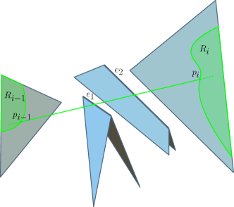
Figure 7: The order of the curves on the boundaries of $R_{i}$ grows with $i$.

Unlike in 2D, the boundaries of $R_{i}$ interior to the faces of $D$ do not necessarily consist of straight-line segments. Observe, that a union of all lines intersecting three given lines in 3D forms a hyperboloid, and therefore, illuminating a straight-line segment on the boundaries of $R_{i-1}$ leads to the corresponding part of $\partial R_{i}$ to be an intersection of a hyperboloid and a plane, i.e., a hyperbola. Moreover, consider some point $p_{i-1}\in\partial R_{i-1}$ interior to some face $f_{i-1}$ of $D$, and two edges $e_{1}$ and $e_{2}$ of the domain $D$ which $p_{i-1}$ sees partially and which will cast a shadow on some face $f_{i}$ of $D$ (refer to Fig. 7). Then we can express the coordinates of $p_{i}$ as:

$$\begin{pmatrix}x_{i}\\ y_{i}\\ z_{i}\end{pmatrix}=\begin{pmatrix}\dfrac{A_{1}x_{i-1}^{2}+B_{1}y_{i-1}^{2}+C_{1}x_{i-1}y_{i-1}+D_{1}x_{i-1}+E_{1}y_{i-1}+F_{1}}{Ax_{i-1}^{2}+By_{i-1}^{2}+Cx_{i-1}y_{i-1}+Dx_{i-1}+Ey_{i-1}+F}\\[12.0pt] \dfrac{A_{2}x_{i-1}^{2}+B_{2}y_{i-1}^{2}+C_{2}x_{i-1}y_{i-1}+D_{2}x_{i-1}+E_{2}y_{i-1}+F_{2}}{Ax_{i-1}^{2}+By_{i-1}^{2}+Cx_{i-1}y_{i-1}+Dx_{i-1}+Ey_{i-1}+F}\\[12.0pt] Ux_{i}+Vy_{i}+W\end{pmatrix}\,,$$ (3)

for some constants $A_{1},A_{2},A,B_{1},\dots,U,V,W$ that depend on the parameters of $f_{i-1}$, $f_{i}$, $e_{1}$, $e_{2}$. Denote a polynomial of degree $d$ as $\mathsf{poly}^{d}(\cdot)$, then we can rewrite the $x$- and the $y$-coordinates of $p_{i}$ as

$$\begin{pmatrix}x_{i}\\ y_{i}\end{pmatrix}=\begin{pmatrix}\dfrac{\mathsf{poly}_{x,i-1}^{2}(x_{i-1},y_{i-1})}{\mathsf{poly}_{i-1}^{2}(x_{i-1},y_{i-1})}\\[12.0pt] \dfrac{\mathsf{poly}_{y,i-1}^{2}(x_{i-1},y_{i-1})}{\mathsf{poly}_{i-1}^{2}(x_{i-1},y_{i-1})}\end{pmatrix}=\begin{pmatrix}\dfrac{\mathsf{poly}_{x,i-2}^{4}(x_{i-2},y_{i-2})}{\mathsf{poly}_{i-2}^{4}(x_{i-2},y_{i-2})}\\[12.0pt] \dfrac{\mathsf{poly}_{y,i-2}^{4}(x_{i-2},y_{i-2})}{\mathsf{poly}_{i-2}^{4}(x_{i-2},y_{i-2})}\end{pmatrix}=\begin{pmatrix}\dfrac{\mathsf{poly}_{x,0}^{2i}(x_{0},y_{0})}{\mathsf{poly}_{0}^{2i}(x_{0},y_{0})}\\[12.0pt] \dfrac{\mathsf{poly}_{y,0}^{2i}(x_{0},y_{0})}{\mathsf{poly}_{0}^{2i}(x_{0},y_{0})}\end{pmatrix}\,,$$

where point $p_{0}(x_{0},y_{0},z_{0})$ lies on some straight-line segment of $\partial D$, and we use different subscripts of the polynomials to distinguish between different expressions. Notice that the denominators of the $x_{i}$ and $y_{i}$ expressed as functions of $x_{j}$ and $y_{j}$ (for all $j<i$) are always the same. If we slide $p_{0}$ along the line segment, and express its coordinates in terms of a parameter $t$, we get

$$x_{i}=\frac{\mathsf{poly}_{x}^{2i}(t)}{\mathsf{poly}^{2i}(t)}\,,\qquad y_{i}=\frac{\mathsf{poly}_{y}^{2i}(t)}{\mathsf{poly}^{2i}(t)}\,,\qquad z_{i}=\mathsf{poly}^{1}(x_{i},y_{i})\,.$$

Thus, the curve, that point $p_{i}$ traces on $f_{i}$ is an intersection of a plane in 3D (face $f_{i}$) and two surfaces of order $2i+1$ in 4D space (with coordinates $x$, $y$, $z$, and $t$). Therefore, the order of that curve is not greater than $2i+1$. In fact, as we have mentioned above, for $i=1$, the curve that $p_{1}$ traces on face $f_{1}$ is a hyperbola, with order $2$, and not $2i+1=3$. The fact that the denominators of the expressions of $x_{1}$ and $y_{1}$ are the same allow to reduce the order of the expressions in the following way:

$$\begin{split}x_{1}&=\frac{\mathsf{poly}_{x}^{2}(t)}{\mathsf{poly}^{2}(t)}=x^{\prime}_{1}+\frac{\mathsf{poly}_{x^{\prime}}^{1}(t)}{\mathsf{poly}^{2}(t)}\,,\\ y_{1}&=\frac{\mathsf{poly}_{y}^{2}(t)}{\mathsf{poly}^{2}(t)}=y^{\prime}_{1}+\frac{\mathsf{poly}_{y^{\prime}}^{1}(t)}{\mathsf{poly}^{2}(t)}\,,\end{split}$$ (4)

Therefore,

$$\frac{x_{1}-x^{\prime}_{1}}{y_{1}-y^{\prime}_{1}}=\frac{\mathsf{poly}_{x^{\prime}}^{1}(t)}{\mathsf{poly}_{y^{\prime}}^{1}(t)}\,,$$

and then

$$t=poly^{1}(x_{1},y_{1})\,.$$

Substituting this expression into Equations 4 we get, that the actual order of the curve traced by $p_{1}$ is $2$. For larger $i$, denominators of the expressions of $x_{i}$ and $y_{i}$ are also equal, however the explicit formula for the curve traced by $p_{i}$ cannot be derived in a similar way. We summarize our findings:

Theorem 9.

The boundaries of region $R_{i}$ are curves of order at most $2i+1$ for $i\geq 2$, and at most $2$ for $i=1$.

The fact that the order of the curves on the boundaries of $R_{i}$ grows linearly may give hope that the bit complexity of representation of $R_{i}$ can be bounded from above similarly to Section 2.2. However, following similar calculations we will get that the space required to store the coordinates of $p_{i}$ grows exponentially with $i$.

Parameters $A_{1},A_{2},A,B_{1},\dots,W$ of Equation 3 have bit complexity not greater than $c\log n$ for some constant $c$ . Let $x_{i-1}$ be represented as a rational number $\raise 2.15277pt\hbox{$p_{x}$}\kern-1.00006pt/\kern-1.49994pt\lower 1.07639pt\hbox{$q_{x}$}$, and $y_{i-1}$ be represented as a rational number $\raise 2.15277pt\hbox{$p_{y}$}\kern-1.00006pt/\kern-1.49994pt\lower 1.07639pt\hbox{$q_{y}$}$, where $p_{x}$ and $q_{x}$, and $p_{y}$ and $q_{y}$ are two pairs of mutually prime integers. Then the number of bits required to represent $x_{i-1}$ is $sp(x_{i-1})\geq\max\{\log p_{x},\log q_{x}\}$. Therefore, the number of bits required to represent $x_{i}$

$$\begin{split}sp(x_{i})\leq&\log(A_{1}p_{x}^{2}q_{y}^{2}+B_{1}q_{x}^{2}p_{y}^{2}+C_{1}p_{x}q_{x}p_{y}q_{y}+D_{1}p_{x}q_{x}q_{y}^{2}+E_{1}q_{x}^{2}p_{y}q_{y}+F_{1}q_{x}^{2}q_{y}^{2})+\\ &\log(Ap_{x}^{2}q_{y}^{2}+Bq_{x}^{2}p_{y}^{2}+Cp_{x}q_{x}p_{y}q_{y}+Dp_{x}q_{x}q_{y}^{2}+Eq_{x}^{2}p_{y}q_{y}+Fq_{x}^{2}q_{y}^{2})\leq\\ \leq&2\log(6Mr^{4})=2\log 6+2\log M+8\log r\leq 6+2c\log n+8\max\{sp(x_{i-1}),sp(y_{i-1})\}\,,\end{split}$$

where $M=\max\{A_{1},B_{1},\dots,E,F\}$ and $r=\max\{p_{x},q_{x},p_{y},q_{y}\}$. Solving the above recurrence we get $sp(x_{i})\leq 9^{i}$, which implies exponential upper bound of the space required to store $x_{i}$.

Lemma 10.

The coordinates of a vertex of $R_{i}$ can be stored in $O(9^{i})$ space.

6 Computational Complexity in $\mathbb{R}^{3}$

We will show now how to use our blueprint from Section 3.1 to build a terrain for the MinLinkPath_1,2 problem such that a path from $s$ to $t$ with $2n-1$ links will exist if and only if there exists a subset $S\subseteq A$ whose sum is equal to half the sum of all integers $A=\{a_{1},\dots,a_{m}\}$. Take the 2D construction and bend it along all the lines $\ell_{i}$ and $\ell^{\prime}_{i}$, except $\ell_{0}$ and $\ell_{m}$ (refer to Fig. 8). Let the angles between consecutive faces be $\pi-\delta$ for some small angle $\delta<\pi/4m$ (so that the sum of bends between the first face (between the lines $\ell_{0}$ and $\ell_{1}$) and the last face (between the lines $\ell^{\prime}_{m}$ and $\ell_{m}$) is less than $\pi$). On each face build a fence of height $\tan(\delta/4)$ according to the 2D construction. The height of the fences is small enough so that no two points on consecutive fences see each other. Therefore, for two points $s$ and $t$ placed on $\ell_{0}$ and $\ell_{m}$ as described above, an $s$-$t$ path with $2m-1$ links must bend only on $\ell_{i}$ and $\ell^{\prime}_{i}$ and pass in the slits in the fences. Finding a min-link path on such a terrain is equivalent to finding a min-link path (with bends restricted to $\ell_{i}$ and $\ell^{\prime}_{i}$) in the 2D construction. Therefore,

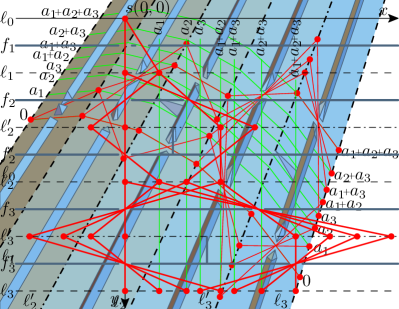
Figure 8: Right: The terrain obtained by bending the 2D construction along the important and intermediate lines. The height of the fences is low enough that no two points on consecutive fences can see each other.

Theorem 11.

MinLinkPath_1,2 on a terrain is NP-hard.

Remark 1.

Instead of $0$-width slits, we could use slits of positive width $w=o(\frac{1}{4m})$; since the width of the light beam grows by $2w$ between two consecutive creases, on the last crease the maximum shift of the path due to the positive slits width will be at most $(2m-1)\times 2w<1$.

Observe that bending in the interior of a face cannot reduce the link distance between $s$ and $t$. Hence, our reduction also shows that MinLinkPath_2,2 is NP-hard. Furthermore, lifting the links from the terrain surface into $\mathbb{R}^{3}$ also does not reduce link distance; we can make sure that the fences are low in height, so that fences situated on different faces of the creased rectangle do not see each other. Therefore, jumping onto the fences is useless. Hence, MinLinkPath_1,3 and MinLinkPath_2,3 are also NP-hard.

MinLinkPath_a,b in general polyhedra

Since a terrain is a special case of a 3D polyhedra, it follows that MinLinkPath_1,2, MinLinkPath_2,2, MinLinkPath_1,3, and MinLinkPath_2,3 are also NP-hard for an arbitrary polyhedral domain in $\mathbb{R}^{3}$. Our construction does not immediately imply that MinLinkPath_3,3 is NP-hard. However, we can put a copy of the terrain slightly above the original terrain (so that the only free space is the thin layer between the terrains). When this layer is thin enough, the ability to take off from the terrain, and bend in the free space, does not help in decreasing the link distance from $s$ to $t$. Thus, MinLinkPath_3,3 is also NP-hard.

Corollary 12.

MinLinkPath_a,b, with $a\geq 1$ and $b\geq 2$, in a 3D domain $D$ is NP-hard. This holds even if $D$ is just a terrain.

7 Algorithmic Results in $\mathbb{R}^{3}$

7.1 Constant-factor Approximation

Our approximations refine and extend the 2-approximation for minimum-link paths in higher dimensions suggested in Chapter 26.5 (section Other Metrics) of the handbook [3] (see also Ch. 6 in [45]); since the suggestion is only one sentence long, we fully quote it here:

Link distance in a polyhedral domain in $\mathbb{R}^{d}$ can be approximated (within factor 2) in polynomial time by searching a weak visibility graph whose nodes correspond to simplices in a simplicial decomposition of the domain.

Indeed, consider $D|^{a}$, the set of all points where the path is allowed to bend, and decompose $D|^{a}$ into a set $F$ of small-complexity convex pieces, and call each piece a feature. Similar to Section 4.2, we say two features $f$ and $f^{\prime}$ are weakly visible if there exist mutually visible points $p\in f$ and $p^{\prime}\in f^{\prime}$; more generally, the weak visibility region $W(f)$ is the set of points that see at least one point of $f$, so $f^{\prime}$ is weakly visible from $f$ iff $f^{\prime}\cap W(f)\neq\varnothing$ (in terms of illumination $W(f)$ is the set of points that get illuminated when a light source is put at every point of $f$). See Fig. 9 for an illustration.

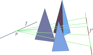
Figure 9: The weak visibility $W(f)$ restricted to edge $f^{\prime}$ is the union of all visible intervals (green) over all points $p\in f$. If this region is non-empty, $f$ and $f^{\prime}$ are weakly visible.

Weak visibility between two features $f$ and $f^{\prime}$ can be determined straightforwardly by building the set of pairs of points $(p,p^{\prime})$ in the parameter space $f\times f^{\prime}$ occluded by (each element of) the obstacles. To be precise, $f\times f^{\prime}$ is a subset of $\mathbb{R}^{2a}$. Now, consider $D|^{d-1}$, which we also decompose into a set of constant-complexity elements. Each element $e$ defines the set $B(e)=\{(p,p^{\prime})\in f\times f^{\prime}:pp^{\prime}\cap e\neq\varnothing\}$ of pairs of points that it blocks; since $e$ has constant complexity, the boundary of $B(e)$ consists of a constant number of curved surfaces, each described by a low degree polynomial. Since there are $O(n)$ elements, the union (and, in fact, the full arrangement) of the sets $B(e)$ for all $e$ can be built in $O(n^{4a-3+\varepsilon})$ time, for an arbitrarily small $\varepsilon>0$, or $O(n^{2})$ time in case $a=1$ [46]. We define the visibility map $M(f,f^{\prime})\subseteq f\times f^{\prime}$ to be the complement of the union of the blocking sets, i.e., the map is the set of mutually visible pairs of points from $f\times f^{\prime}$. We have:

Lemma 13.

$M(f,f^{\prime})$ can be built in $O(n^{\max(2,4a-3+\varepsilon)})$ time, for an arbitrarily small $\varepsilon>0$.

The features $f$ and $f^{\prime}$ weakly see each other iff $M(f,f^{\prime})$ is not empty. Let $G$ be the graph on features whose edges connect weakly visible features; $s$ and $t$ are added as vertices of $G$, connected to features (weakly) seen from them. Let $\pi=\{f_{0},f_{1},\dots,f_{\ell}\}$, with $f_{0}=s$ and $f_{\ell}=t$ be a shortest $s$-$t$ path in $G$; $\ell$ is the length of $\pi$. Embed edges of $\pi$ into the geometric domain, putting endpoints of the edges arbitrarily into the corresponding features. This does not necessarily connect $s$ to $t$ since it could be that, inside a feature $f_{i}$, the endpoint of the edge $f_{i-1}f_{i}$ does not coincide with endpoint of the edge $f_{i}f_{i+1}$; to create a connected path, connect the two endpoints by an extra link within $f_{i}$ (this is possible since the features are convex).

Bounding the approximation ratio of the above algorithm is straightforward: Let $\mathsf{opt}$ denote a min-link $s$-$t$ path and, abusing notation, also the number of links in it. Consider the features to which consecutive bends of $\mathsf{opt}$ belong; the features are weakly visible and hence are adjacent in $G$. Thus $\ell\leq\mathsf{opt}$. Adding the extra links inside the features adds at most $\ell-1$ links. Hence the total number of links in the produced path is at most $2\ell-1<2\mathsf{opt}$.

Since $G$ has $O(n)$ nodes and $O(n^{2})$ edges, Dijkstra’s algorithm will find the shortest path in it in $O(n^{2})$ time.

Theorem 14.

(cf. [3, Ch. 27.5].) A 2-approximation to MinLinkPath_a,b can be found in $O(n^{2+\max(2,4a-3+\varepsilon)})$ time, where $\varepsilon>0$ is an arbitrarily small constant.

Interestingly, the running time in Theorem 14 depends only on $a$, and not on $b$ or $d$, the dimension of $D$ (of course, $a\leq d$, so the runtime is bounded by $O(n^{2+\max(2,4d-3+\varepsilon)})$ as well).

7.2 PTAS

To get a $(1+1/k)$-approximation algorithm for any constant $k\geq 1$, we expand the above handbook idea by searching for shortest $s$-$t$ path $\pi^{k}$ in the graph $G^{k}$ whose edges connect features that are $k$-link weakly visible. Similarly to Section 4.2, we obtain the following.

Theorem 15.

For a constant $k$ the path $\pi^{k}_{*}$, having at most $(1+1/k)\mathsf{opt}$ links, can be constructed in polynomial time.

Proof.

The approximation factor follows from the same argument as in Section 4.2. To show the polynomial running time, we argue that the weak $k$-link visibility between features can be determined in polynomial time using the staged illumination: starting from each feature $f$, find the set $W(f)$ of points on other features weakly visible from $f$, then find the set weakly visible from $W^{2}(f)=W(W(f))$, repeat $k$ times to obtain the set $W^{k}(f)$ reachable from $f$ with $k$ links; feature $f^{\prime}$ can be reached from $f$ in $k$ links iff $W^{k}(f)\cap f^{\prime}\neq\varnothing$. For constant $k$, building $W^{k}(f)$ takes time polynomial in $n$, although possibly exponential in $k$ (in fact, for diffuse reflection explicit bounds on the complexity of $W^{k}(f)$ were obtained [36, 37, 10]). This can be seen by induction: Partition the set $W^{i-1}(f)$ into the polynomial number of constant-complexity pieces. For each piece $p$, each element $e$ of the boundary of the domain and each feature $f^{\prime}$ compute the part of $f^{\prime}$ shadowed by $e$ from the light sources on $p$—this can be done in constant time analogously to determining weak visibility between two features above (by considering the part of $p\times f^{\prime}$ carved out by the occluder $e$). The part of $f^{\prime}$ weakly seen from $W^{i-1}(f)$ is the union, over all parts $p$, of the complements of the sets occluded by all elements $e$; since there is a polynomial number of parts, elements and features, it follows that $W^{i}(f)$ can be constructed in polynomial time. ∎

7.3 The global visibility map of a terrain

Using the result from Theorem 14 for MinLinkPath_2,3 on terrains, we get a 2-approximate min-link path in $O(n^{7+\varepsilon})$ time (since the path can bend anywhere on a triangle of the terrain, the features are the triangles and intrinsic dimension $d=2$). In this section we show that a faster, $O(n^{4})$-time 2-approximation algorithm is possible. We also consider encoding visibility between all points on a terrain (not just between features, as the visibility map from Section 7 does): we give an $O(n^{4})$-size data structure for that, which we call the terrain’s global visibility map, and provide an example showing that the size of the structure is worst-case optimal.

We start with connecting approximations of MinLinkPath_2,3 and MinLinkPath_1,3 on terrains. Let $\mathsf{opt}$ be an optimal solution in an instance of MinLinkPath_2,3, let $\mathsf{opt}_{e}$ be the optimal solution to MinLinkPath_1,3 in the same instance, and let $\mathsf{apx}_{e}$ be the 2-approximate path for the MinLinkPath_1,3 version output by the algorithm in Section 7 (Theorem 14); abusing notation, let $\mathsf{opt}$, $\mathsf{opt}_{e}$ and $\mathsf{apx}_{e}$ denote also the number of links in the paths. Clearly, $\mathsf{apx}_{e}\leq 2\mathsf{opt}_{e}$; what we show is that actually a stronger inequality holds (the inequality is stronger since $\mathsf{opt}\leq\mathsf{opt}_{e}$):

Lemma 16.

$\mathsf{apx}_{e}\leq 2\mathsf{opt}$.

Proof.

Consider some link $pq$ on optimal path $\mathsf{opt}$ from $s$ to $t$. Draw a vertical plane through $p$ and $q$ and denote as $p^{\prime}$ and $q^{\prime}$ the uppermost intersections of this plane with the boundaries of the triangles containing $p$ and $q$ (refer to Fig. 10). Then $p^{\prime}$ and $q^{\prime}$ see each other, and they lie on edges of the terrain.

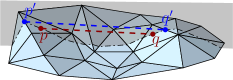
Figure 10: For every pair of points $p\in f_{p}$ and $q\in f_{q}$ that can see each other, there exist points $p^{\prime}$ and $q^{\prime}$ on the edges bounding $f_{p}$ and $f_{q}$, respectively, that can also see each other.

Replace every link $pq$ of $\mathsf{opt}$ by $p^{\prime}q^{\prime}$, and interconnect the consecutive links by straight segments. Such interconnecting segments will belong to an edge of the terrain, or go through the interior of a triangle containing the corresponding vertex of the optimal path. The resulting chain of edges is a proper path from $s$ to $t$ whose bends lie only on edges of the terrain. Thus, it has a corresponding path in graph $G$ (refer to Theorem 14). The length of such a path is at most $2\mathsf{opt}-1$, and it is not shorter than $\mathsf{apx}_{e}$ (the shortest path in $G$). Therefore, $\mathsf{apx}_{e}\leq 2\mathsf{opt}$.

∎

Lemma 16 allows us to use the 2-approximation for MinLinkPath_1,3 as a 2-approximation for MinLinkPath_2,3. The former can be found more efficiently: by Theorem 14, $\mathsf{apx}_{e}$ can be found in $O(n^{4})$ time.

Theorem 17.

A 2-approximation for MinLinkPath_2,3 in a terrain can be found in $O(n^{4})$ time.

The running time of the algorithm in Theorem 17 is dominated by determining weak visibility between all $\binom{n}{2}$ pairs of edges; the approach from Section 7 does it with brute force in $O(n^{2})$ time per pair. An obvious question is whether this could be done faster for a single pair. We now show that this is hardly the case. We start from the analogous result for 2D polygonal domains:

Theorem 18.

Determining weak visibility between a pair of edges in a polygonal domain with holes is 3SUM-hard.

Proof.

The proof is by picture; see Fig. 11. ∎

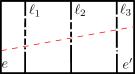
Figure 11: Start from an instance of the 3SUM-hard problem GeomBase [47]: Given a set $S$ of points lying on 3 parallel lines $\ell_{1},\ell_{2},\ell_{3}$, do there exist 3 points from $S$ lying on a line $\ell\notin\{\ell_{1},\ell_{2},\ell_{3}\}$? Construct an instance of the weak visibility problem for edges $e,e^{\prime}$ in a polygonal domain: $\ell_{1},\ell_{2},\ell_{3}$ become obstacles and each point $p\in S$ is a gap punched in the obstacle; the lines are in a box whose two opposite edges (parallel to the lines) are the edges $e,e^{\prime}$. The edges are weakly visible iff there exist 3 collinear gaps $p_{i},i=1,2,3$, such that $p_{i}\in\ell_{i}$.

The domain in Fig. 11 can be turned into a terrain by erecting the lines $\ell_{1},\ell_{2},\ell_{3}$ into 3 vertical walls (the gaps in the lines become slits in the walls); similarly to the 2D case, the edges $e,e^{\prime}$ weakly see each other iff GeomBase is feasible:

Theorem 19.

Determining weak visibility between a pair of edges in a terrain is 3SUM-hard.

The above 3SUM-hardness results are not the end of the story: the fact that determining weak visibility for a single pair of edges may require quadratic time does not imply that determining the visibility between all pairs of edges should require quatric time. In fact, the 3SUM-hardness of the 2D case (Theorem 18) does not preclude existence of $O(n^{2})$-time algorithm for finding all pairs of weakly visible edges in a polygonal domain with holes—such an algorithm is used, e.g., in Section 4 of [1]. Moreover, in [48] it is shown that a data structure of $O(n^{2})$ size can be built in $O(n^{2})$ time, encoding visibility between all pairs of points in a domain; the data structure, which can be called the global visibility map of the domain, is an extension of the standard visibility graph that encodes visibility only between the domain’s vertices. An immediate question is whether such a data structure can be built for terrains; below is our answer.

The global visibility map that encodes all mutually visible pairs of points on a terrain (or in a full 3D domain) will live in four dimensions—this is because a line in $\mathbb{R}^{3}$ has four degrees of freedom, and our data structure will use the projective dual $4D$ space $\mathcal{S}_{d}$ to the primary 3D space $\mathcal{S}_{p}$ where the terrain is located. A line $\ell\in\mathcal{S}_{p}$ will correspond to a point $\ell^{*}\in\mathcal{S}_{d}$. To build the global visibility map, consider a $5D$ space $\mathcal{S}_{5}$ where $\mathcal{S}_{p}$ and $\mathcal{S}_{d}$ are subspaces, and a point $O$ in $\mathcal{S}_{5}$ with coordinates $(0,0,0,0,1)$. The dual point $\ell^{*}\in\mathcal{S}_{d}$ for a line $\ell\in\mathcal{S}_{p}$ is constructed as follows: Draw a $4D$ hyperplane in $\mathcal{S}_{5}$ that goes through line $\ell$ and point $O$. A perpendicular line to such hyperplane that goes through $O$ intersects $\mathcal{S}_{d}$ in a point. This point will be $\ell^{*}$—the dual point to line $\ell$.

Now, the visibility map is a partition of $\mathcal{S}_{d}$ into cells, such that each cell contains points whose duals have the same combinatorial structure, i.e., they intersect the same set of obstacles’ faces in $\mathcal{S}_{p}$.

Lemma 20.

The global visibility map that encodes all pairs of mutually visible points on terrain $T$ (or on a set of obstacles $\mathcal{O}$ in full 3D model) has complexity $O(n^{4})$.

Proof.

Let $\mathcal{L}$ be a set of $n$ lines in $\mathcal{S}_{p}$. $\mathcal{L}$ implies a subdivision $W$ of space $\mathcal{S}_{d}$ into cells that correspond to lines that touch the same sets of lines in $\mathcal{L}$. $W$ consists of $0$-cells (vertices), $1$-cells (edges), $2$-cells, $3$-cells, and $4$-cells. The $k$-cells of $W$ correspond to a set of lines that intersects exactly $4-k$ lines of $\mathcal{L}$. There are clearly $O(n^{4})$ $0$-cells, since there are $n$ lines in $\mathcal{L}$. For each $k$-cell, the number of incident $(k+1)$-cells is $O(1)$, since they correspond to the sets of lines we get by dropping incidence to $1$ of the $4-k$ lines (and $4-k$ is constant). Therefore, the number of $k$-cells is also bounded by $O(n^{4})$ for all $k$. Hence, $W$ has complexity $O(n^{4})$.

Now, consider our terrain $T$ (or a set of obstacles $\mathcal{O}$ in full 3D model) in $\mathcal{S}_{p}$. We are interested in the subdivision $S$ of $\mathcal{S}_{d}$ into cells that correspond to line segments that are combinatorially equal (their end points are on the same features of $T$ or $\mathcal{O}$). Then, $W$ is a sub-subdivision of $S$ (in the sense of subgraph, so something with fewer components). Hence, $S$ also has complexity $O(n^{4})$. ∎

Remark. The first part of the above argument (the complexity of configuration space of lines among lines in $3$-space) is a natural question and it is well-studied. McKenna and O’Rourke [49] argue quartic bounds on the numbers of $0$-faces, $1$-faces and $4$-faces (although many proofs in their paper are omitted). They also describe how to compute the complex consisting of all $0$-faces and $1$-faces in $O(n^{4}\alpha(n))$ time.

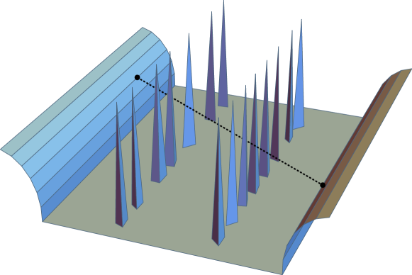
Figure 12: Every vertex (0-face) in the visibility map corresponds to a line that crosses $4$ edges of the terrain. In this example, there is a line that connects any horizontal edge on the left-hand side with any horizontal segment on the right-hand side, and that also pins two spikes in the middle. Thus, there are $\Omega(n^{4})$ $0$-faces in the visibility map.

We now argue that the bound in Lemma 20 is tight: the global visibility map may have complexity $\Omega(n^{4})$. (Other then possibly being an interesting result by itself,) this implies, in particular, that the running time of the algorithm in Theorem 17 may not be improved if one were to compute the weak visibility between all pairs of edges.

Lemma 21.

The global visibility map that encodes all pairs of mutually visible points on terrain $T$ can have complexity $\Omega(n^{4})$.

Proof.

See Fig. 12. It is easy to see that this construction yields a visibility map of complexity $\Omega(n^{4})$. ∎

Lemmas 20 and 21 give tight bounds on the complexity of the visibility map:

Theorem 22.

The complexity of global visibility map, encoding all pairs of mutually visible points on terrain (or on a set of obstacles in 3D) of complexity $n$, is $\Theta(n^{4})$.

8 Lower bound constructions for MinLinkPath_0,3 on terrains

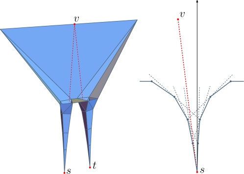
Figure 13: On terrains, MinLinkPath_0,3 may be a factor $\Omega(n)$ worse than MinLinkPath_1,3. In the example shown, a solution to MinLinkPath_0,3 requires $\Omega(n)$ links, whereas MinLinkPath_1,3 requires only two. Left: The 3D view on the trenches. Point $v$ is seen from both $s$ and $t$. Right: A cross-section of a trench. Vertices of each layer $i$ cannot see any other vertex further than the next layer.

Consider a terrain with two deep trenches whose vertices come in layers, see for example Fig. 13. Vertices in layer $i$ are connected to the vertices of the previous layer, $i-1$, and vertices of the next layer, $i+1$. Moreover, the only vertices visible from vertices in layer $i$ are the ones in layers $i-1$ and $i+1$. Place $s$ and $t$ at the bottom of the trenches. An $s\textrm{-}t$ path restricted to bend only at vertices of the terrain will have a bend at each layer of the trenches, and therefore will have $\Omega(n)$ links.

Now, place a tall steep face right outside the trenches, such that no vertices of it can bee seen from any of the vertices inside the trenches, but some of its interior and boundary edge $e$ can be seen from both $s$ and $t$. Then, a solution to MinLinkPath_1,3 may bend in a point $v$ on $e$, and thus reach $t$ with two links. Thus:

Proposition 1.

There is a terrain $\mathbb{T}$ of $n$ vertices, and two vertices $s$ and $t$ on $\mathbb{T}$, such that a solution to MinLinkPath_0,3 requires $\Omega(n)$ times as much links as a solution to MinLinkPath_1,3.

9 Conclusion

We considered minimum-link paths in 3D, showing that most of the versions of the problem are hard but admit PTASes; we also obtained similar results for the diffuse reflection problem in 2D polygonal domains with holes. The biggest remaining open problem is whether pseudopolynomial-time algorithms are possible for the problems: our reductions are from 2-PARTITION, and hence do not show strong hardness. A related question is exploring bit complexity of the min-link paths in 3D (note that already in 2D simple polygons finding min-link path with integer vertices is weakly NP-hard [50]).

Acknowledgments

We thank Joe Mitchell and Jean Cardinal for fruitful discussions on this work and the anonymous reviewers for their helpful comments. M.L. and I.K. are supported by the Netherlands Organisation for Scientific Research (NWO) under grants 639.021.123 and 639.023.208 respectively. V.P. is supported by grant 2014-03476 from the Sweden’s innovation agency VINNOVA. F.S. is supported by the Danish National Research Foundation under grant nr. DNRF84.

References

- [1] Subir Kumar Ghosh, Partha P. Goswami, Anil Maheshwari, Subhas C. Nandy, Sudebkumar Prasant Pal and Swami Sarvattomananda “Algorithms for computing diffuse reflection paths in polygons” In The Visual Computer 28.12, 2012, pp. 1229–1237 DOI: 10.1007/s00371-011-0670-z
- [2] J.S.B. Mitchell, G. Rote and G. Woeginger “Minimum-link paths among obstacles in the plane” In Algorithmica 8.1 Springer, 1992, pp. 431–459
- [3] J. E. Goodman and J. O’Rourke “Handbook of Discrete and Computational Geometry”, CRC Press series on discrete mathematics and its applications Chapman & Hall/CRC, 2004
- [4] Erik D. Demaine, Joseph S. B. Mitchell and Joseph O’Rourke “The Open Problems Project”, http://maven.smith.edu/~orourke/TOPP/
- [5] Subhash Suri “A linear time algorithm with minimum link paths inside a simple polygon” In Computer Vision, Graphics and Image Processing 35.1 San Diego, CA, USA: Academic Press Professional, Inc., 1986, pp. 99–110 DOI: http://dx.doi.org/10.1016/0734-189X(86)90127-1
- [6] Subir Kumar Ghosh “Computing the Visibility Polygon from a Convex Set and Related Problems” In Journal of Algorithms 12.1, 1991, pp. 75–95
- [7] John Hershberger and Jack Snoeyink “Computing Minimum Length Paths of a Given Homotopy Class” In Computational Geometry: Theory and Applications 4, 1994, pp. 63–97
- [8] Simon Kahan and Jack Snoeyink “On the bit complexity of minimum link paths: Superquadratic algorithms for problems solvable in linear time” In Computational Geometry: Theory and Applications 12.1-2, 1999, pp. 33–44
- [9] Joseph S. B. Mitchell, Valentin Polishchuk and Mikko Sysikaski “Minimum-link paths revisited” In Computational Geometry 47.6, 2014, pp. 651–667 DOI: 10.1016/j.comgeo.2013.12.005
- [10] Boris Aronov, Alan R. Davis, John Iacono and Albert Siu Cheong Yu “The Complexity of Diffuse Reflections in a Simple Polygon” In Proc. 7th Latin American Symposium on Theoretical Informatics, 2006, pp. 93–104
- [11] Leonidas J. Guibas, John Hershberger, Joseph S. B. Mitchell and Jack Snoeyink “Approximating Polygons and Subdivisions with Minimum Link Paths” In Proceedings of the 2Nd International Symposium on Algorithms, ISA ’91 London, UK, UK: Springer-Verlag, 1991, pp. 151–162 URL: http://dl.acm.org/citation.cfm?id=648003.743125
- [12] C. D. Yang, D. T. Lee and C. K. Wong “Rectilinear paths problems among rectilinear obstacles revisited” In SIAM Journal on Computing 24, 1995, pp. 457–472
- [13] C. D. Yang, D. T. Lee and C. K. Wong “On bends and distances of paths among obstacles in 2-layer interconnection model” In IEEE Transactions on Computing 43.6, 1994, pp. 711–724
- [14] C. D. Yang, D. T. Lee and C. K. Wong “On bends and lengths of rectilinear paths: a graph theoretic approach” In International Journal of Computational Geometry & Applications 2.1, 1992, pp. 61–74
- [15] John Adegeest, Mark H. Overmars and Jack Snoeyink “Minimum-link -oriented paths: Single-source queries” In Int. J. of Computational Geometry and Applications 4.1, 1994, pp. 39–51
- [16] Leonidas J. Guibas, J. Hershberger, D. Leven, Micha Sharir and R. E. Tarjan “Linear-time algorithms for visibility and shortest path problems inside triangulated simple polygons” In Algorithmica 2, 1987, pp. 209–233
- [17] J. Hershberger and J. Snoeyink “Computing minimum length paths of a given homotopy class” In Computational Geometry: Theory and Applications 4, 1994, pp. 63–98
- [18] Moshe Dror, Alon Efrat, Anna Lubiw and Joseph S. B. Mitchell “Touring a Sequence of Polygons” In Proceedings of the Thirty-fifth Annual ACM Symposium on Theory of Computing, STOC ’03 San Diego, CA, USA: ACM, 2003, pp. 473–482 DOI: 10.1145/780542.780612
- [19] Svante Carlsson, Håkan Jonsson and Bengt J Nilsson “Finding the shortest watchman route in a simple polygon” In Discrete & Computational Geometry 22.3 Springer-Verlag, 1999, pp. 377–402
- [20] Joseph SB Mitchell “Approximating watchman routes” In Proc. 24th Annual ACM-SIAM Symposium on Discrete Algorithms, 2013, pp. 844–855 SIAM
- [21] M. H. Alsuwaiyel and D. T. Lee “Minimal link visibility paths inside a simple polygon” In Comput. Geom. Theory Appl. 3.1, 1993, pp. 1–25
- [22] Mark Berg “Generalized hidden surface removal” In Computational Geometry 5.5, 1996, pp. 249–276 DOI: http://dx.doi.org/10.1016/0925-7721(95)00008-9
- [23] Joseph S. B. Mitchell and Micha Sharir “New Results on Shortest Paths in Three Dimensions” In Procedings of the 20th Annual Symposium on Computational Geometry Brooklyn, New York, USA: ACM, 2004, pp. 124–133 DOI: 10.1145/997817.997839
- [24] Leila De Floriani and Paola Magillo “Algorithms for visibility computation on terrains: a survey” In Environment and Planning B: Planning and Design 30.5, 2003, pp. 709–728 URL: http://EconPapers.repec.org/RePEc:pio:envirb:v:30:y:2003:i:5:p:709-728
- [25] A. James Stewart “Hierarchical Visibility in Terrains” In Eurographics Rendering Workshop, 1997
- [26] Frank Kammer, Maarten Löffler, Paul Mutser and Frank Staals “Practical Approaches to Partially Guarding a Polyhedral Terrain” In Geographic Information Science Springer, 2014, pp. 318–332
- [27] Boaz Ben-Moshe, Paz Carmi and Matthew J. Katz “Approximating the Visible Region of a Point on a Terrain” In GeoInformatica 12.1, 2008, pp. 21–36 DOI: 10.1007/s10707-006-0017-5
- [28] Boaz Ben-Moshe, Matthew J. Katz, Joseph S. B. Mitchell and Yuval Nir “Visibility preserving terrain simplification—an experimental study” In Comput. Geom. 28.2-3, 2004, pp. 175–190 DOI: 10.1016/j.comgeo.2004.03.005
- [29] Ferran Hurtado, Maarten Löffler, Inês Matos, Vera Sacristán, Maria Saumell, Rodrigo I Silveira and Frank Staals “Terrain visibility with multiple viewpoints” In Proc. 24th International Symposium on Algorithms and Computation Springer, 2013, pp. 317–327
- [30] Esther Moet “Computation and complexity of visibility in geometric environments”, 2008
- [31] Alon Efrat, Leonidas J. Guibas, Olaf A. Hall-Holt and Li Zhang “On incremental rendering of silhouette maps of a polyhedral scene” In Computational Geometry 38.3, 2007, pp. 129–138
- [32] Giovanni Viglietta “Face-Guarding Polyhedra” In CCCG 2011
- [33] M. Berg, M. J. Kreveld, B. J. Nilsson and M. H. Overmars “Shortest path queries in rectilinear worlds” In IJCGA 3.2, 1992, pp. 287–309
- [34] D. Prasad, S. P. Pal and T. Dey “Visibility with multiple diffuse reflections” In Computational Geometry: Theory and Applications 10, 1998, pp. 187–196
- [35] Arijit Bishnu, Subir Kumar Ghosh, Partha P. Goswami, Sudebkumar Prasant Pal and Swami Sarvattomananda “An Algorithm for Computing Constrained Reflection Paths in Simple Polygon”, http://arxiv.org/abs/1304.4320, 2013
- [36] Boris Aronov, Alan R. Davis, Tamal K. Dey, Sudebkumar Prasant Pal and D. Chithra Prasad “Visibility with One Reflection” In Discrete & Computational Geometry 19.4, 1998, pp. 553–574 DOI: 10.1007/PL00009368
- [37] Boris Aronov, Alan R. Davis, Tamal K. Dey, Sudebkumar Prasant Pal and D. Chithra Prasad “Visibility with Multiple Reflections” In Discrete & Computational Geometry 20.1, 1998, pp. 61–78 DOI: 10.1007/PL00009378
- [38] James D. Foley, Richard L. Phillips, John F. Hughes, Andries van Dam and Steven K. Feiner “Introduction to Computer Graphics” Addison-Wesley Longman Publishing Co., Inc., 1994
- [39] Arnold Schönhage “On the power of random access machines” In Proceedings of the 6th Colloquium on Automata, Languages and Programming (ICALP), 1979, pp. 520–529
- [40] Merrick Furst, James B. Saxe and Michael Sipser “Parity, circuits, and the polynomial-time hierarchy” In Math. Systems Theory 17.1, 1984, pp. 13–27
- [41] Michael L. Fredman and Dan E. Willard “Trans-dichotomous algorithms for minimum spanning trees and shortest paths” In Journal of Computer and System Sciences 48.3, 1994, pp. 533–551
- [42] Dania El-Khechen, Muriel Dulieu, John Iacono and Nikolaj Omme “Packing unit squares into grid polygons is NP-complete” In CCCG 2009
- [43] Marcus Schaefer, Eric Sedgwick and Daniel Stefankovic “Recognizing string graphs in NP” In J. Comput. Syst. Sci. 67.2, 2003, pp. 365–380 DOI: 10.1016/S0022-0000(03)00045-X
- [44] J. Canny and J. H. Reif “New lower bound techniques for robot motion planning problems” In Proc. 28th Annual Symposium on Foundations of Computer Science, 1987, pp. 49–60
- [45] Christine Piatko “Geometric bicriteria optimal path problems”, 1993
- [46] Pankaj K Agarwal and Micha Sharir “Arrangements and their applications” In Handbook of computational geometry, 2000, pp. 49–119
- [47] Anka Gajentaan and Mark H. Overmars “On a Class of Problems in Computational Geometry” In Computational Geometry: Theory and Applications 5, 1995, pp. 165–185
- [48] K. Buchin, I. Kostitsyna, M. Löffler and R.I. Silveira “Region-based approximation of probability distributions (for visibility between imprecise points among obstacles)” In Proc. 17th Workshop on Algorithm Engineering and Experiments, 2015
- [49] Michael McKenna and Joseph O’Rourke “Arrangements of Lines in 3-space: A Data Structure with Applications” In Proc. 4th Annual Symposium on Computational Geometry, SCG’88 Urbana-Champaign, Illinois, USA: ACM, 1988, pp. 371–380 DOI: 10.1145/73393.73431
- [50] Wei Ding “On Computing Integral Minimum Link Paths in Simple Polygons” In EuroCG, 2008