Effective string description of confining flux tubes

Abstract

We review the current knowledge about the theoretical foundations of the effective string theory for confining flux tubes and the comparison of the predictions to pure gauge lattice data. A concise presentation of the effective string theory is provided, incorporating recent developments. We summarize the predictions for the spectrum and the profile/width of the flux tube and their comparison to lattice data. The review closes with a short summary of open questions for future research.

11.15.Ha,11.25.Pm,11.30.Cp,12.10.Dm,12.38.Aw,12.40.Nn

1 Introduction

Confinement is one of the most fundamental properties of Quantum Chromodynamics (QCD). Yet, assured knowledge about its microscopic nature is still lacking (e.g. Greensite:2003bk). A possible mechanism to explain quark confinement is the formation of a tube of strong chromoelectric flux between quark $q$ and antiquark $\bar{q}$ (for a mesonic boundstate), leading to a linearly rising potential with the $q\bar{q}$ distance $R$. The emergence of this picture has been triggered by the observation that the square masses of the low lying hadrons, when grouped in so called Regge-trajectories, show a linear increase with the spin. A simplistic model to explain this assumes that mesons consist of a rotating energy string (e.g. Greensite:2003bk,Bali:2000gf). This observation, among others, led to the formulation of the first string theories [3, 4]. Contact to QCD can be made if the region with large field strength density is squeezed into a flux tube with approximately negligible width. Evidence for this effect can be found analytically at strong coupling on the lattice [5, 6, 7]. The flux tube dynamics at large distances would then be governed by a low energy effective string theory (EST) [8, 9, 10].

In the dual-superconductor model for confinement (see Baker:1991bc), the flux tube appears as the generalization of Abrikosov vortices of type II superconductors, following the proposal from Nielsen:1973cs, due to the condensation of chromomagnetic monopoles [13, 14, 15]. Vortex and string pictures have distinct features. The vortex picture predicts an exponential decrease of the field strength at the border of its core with a constant penetration length, while the EST predicts a Gaussian shape and a logarithmic growths of the width [16] with $R$. Nonetheless, the reality is possibly somewhere in between, meaning that the flux tube consists of a solid, vortex-like, inner core, whose long-distance dynamics is governed by the EST.

Historically, there are two main frameworks for the construction of the EST. The static gauge approach, pioneered by Lüscher and Weisz [9, 17, 18] (LW), favors an explicitly unitary description, while the orthogonal gauge formalism, introduced by Polchinski and Strominger [19] (PS), leads to a more symmetric action, but introduces non physical degrees of freedom. The relation between the two has been recently elucidated.[20, 21] The properties of long flux tubes can be investigated in lattice simulations of pure gauge theories, where the absence of dynamical quarks prohibits string breaking. The continuum limit (lattice spacing $a\to 0$) corresponds to the weak coupling limit. In going from strong to weak coupling, the theory passes through a roughening phase transition, across which the continuum symmetries are effectively restored.[17] Simulations have to be done in the continuum phase. Since the first simulations early in the 80‘s [22, 23, 24, 25, 26, 27], they have reached a precision which allows to resolve non-universal terms in the EST. Note, however, that the potential in the real world will be affected by the presence of dynamical quarks.

The review is organized as follows: In the next section we will discuss the construction of the EST, with particular emphasis on recent developments. Section 3 is devoted to the EST predictions concerning the spectrum and the width of the flux tube and in section 4 we discuss the comparison to lattice data. We will conclude with a summary and discussion, where we try to identify relevant open questions and ideas for future research. Limitations in space urged us to subjectively pick topics from a vast field. We would like to apologize to all those whose contribution has not been appreciated sufficiently. A small remark on related topics is included after the conclusions.

2 The effective action for a long confining string

Our aim is to write down the low energy effective field theory (EFT) for stable non-interacting confining flux tubes. Two possible realizations are a flux tube stretched between two static sources or a closed flux tube wrapping around a compactified dimension, rendering it stable under contraction. The latter does not appear in real world QCD, but can be realized at finite volume on the lattice. Since a long flux tube is approximately a one-dimensional object, the EFT will be a two dimensional theory, taking the usual form of a derivative expansion. The degrees of freedom are the Goldstone bosons (GB) associated with the breaking of the translational symmetry by the tube, i.e. the quantized transverse oscillation modes. They carry a minimal energy of $O(R^{-1})$, so that the EFT is accurate for long flux tubes.

The EST is expected to break down at some scale of order $\Lambda_{\textup{QCD}}$ (i.e. $\sqrt{\sigma}R\gtrsim 1$ – see below). String breaking and (virtual) glueball emission are not accounted for. Both processes are suppressed at large $N$, and on-shell glueball emission also at low energies. More massless particles may arise if additional symmetries are broken by the string, as for instance supersymmetry. Weakly coupled light massive modes, if present, can be added to the action as well (see sec. 3.1). Sometimes the effective action can be derived explicitly, by matching to a weakly coupled UV completion,[28] or in cases in which a weakly curved holographic background is available.[29, 30]

2.1 Lorentz symmetry and the effective string action.

We consider a flux tube which extends in the $(x^{0},x^{1})$ plane. We use indices $\mu,\nu,\ldots$ for the full $D$-dimensional space, indices $\alpha,\beta,\ldots$ for the $(0,1)$ plane and latin ones $i,j,\ldots$ for the $D-2$ transverse directions. The action for the GB, which we denote $X^{i}$, retains an $ISO(1,1)\times SO(D-2)$ symmetry group, combining Poincaré symmetry on the worldsheet and rotational symmetry in the transverse directions. Under transverse translations $X^{i}\to X^{i}+\epsilon^{i}$, so the GB couple derivatively. When constructing the action, one can omit terms proportional to lower order equations of motion (EOM), which can be swept to higher orders by field redefinitions. Thus, for a worldsheet $\mathcal{M}$ the first few terms in the action are

$$S_{\textup{bulk}}=\int_{\mathcal{M}}\!\!\displaystyle\big{[}-\sigma-\frac{\sigma}{2}\,\partial_{\alpha}X^{i}\partial^{\alpha}X^{i}+c_{2}(\partial_{\alpha}X^{i}\partial^{\alpha}X^{i})^{2}+c_{3}(\partial_{\alpha}X^{i}\partial_{\beta}X^{i})^{2}\\ \>\>\>\displaystyle+c_{4}(\partial_{\alpha}\partial_{\beta}X^{i}\partial^{\alpha}\partial^{\beta}X^{i})(\partial_{\gamma}X^{j}\partial^{\gamma}X^{j})\dots\big{]}.$$ (1)

Here $\sigma$ is the string tension, governing the linear rise of the potential, which for SU(3) in $D=4$ assumes a value of $\sigma^{-1/2}\approx 0.42$ fm [31]. This value is used to convert to physical units in the following, even when we are in an unphysical situation. Open flux tubes end on static sources, leading to an additional boundary action, constrained by Dirichlet boundary conditions ($\partial_{\parallel}X^{i}=0$). The first terms are

$$S_{\textup{boundary}}=\!\displaystyle\int_{\partial\mathcal{M}}\!\big{[}\mu+b_{1}\partial_{\perp}X^{i}\partial_{\perp}X^{i}\!+b_{2}\partial_{\parallel}\partial_{\perp}X^{i}\partial_{\parallel}\partial_{\perp}X^{i}+b_{3}(\partial_{\perp}X^{i}\partial_{\perp}X^{i})^{2}\dots\big{]}$$ (2)

The string also breaks Lorentz transformations in mixed directions $(\alpha,i)$, which must be nonlinearly realized as well (no additional GB are required[32]). The consequent constraints on the coefficients $b_{i}$ and $c_{i}$ were first investigated via open-closed duality[18] (see also Cohn:1992nu). While this method only exploits $SO(D-2,1)$ invariance,[34, 30] Lorentz invariance can be implemented directly in the action, in line with the standard EFT construction.[35, 36, 37] One constructs fields which, under $ISO(D-1,1)$, only change via a field (i.e. also coordinate) dependent element of the unbroken subgroup.[35] These are the induced metric on the worldsheet $g_{\alpha\beta}=\partial_{\alpha}X^{\mu}\partial_{\beta}X_{\mu}$ and the extrinsic curvature $K_{\alpha\beta}^{I}=n^{I}_{\mu}\nabla_{\alpha}\partial_{\beta}X^{\mu}$, where $X^{\mu}=(x^{\alpha},X^{i})$ and $n^{\mu}_{I}$ is a $(D-2)$-tuple of normal vectors. A Lorentz transformation in the plane $(\alpha,i)$ acts as a diffeomorphism on the worldsheet coordinate, $\delta x^{\alpha}=\epsilon^{\alpha}{}_{i}X^{i}(x)$, so the bulk effective action is diffeomorphism invariant, i.e.

$$S_{\textup{bulk}}=-\int_{\mathcal{M}}\sqrt{-\textup{det}g}\left(\sigma+\alpha\,K_{\alpha\beta}^{I}K^{\alpha\beta}_{I}+\dots\right).$$ (3)

Contrary to eq. (1), worldsheet indices are here contracted through $g^{\alpha\beta}$. The boundary action can be constrained similarly,[18, 42] leading to $b_{1}=b_{3}=0$. The first addend in $S_{\textup{bulk}}$ is the Nambu-Goto (NG) action,[3, 8] whose expansion fixes the $c_{i}$ in eq. (1). In particular, the $c_{4}$ term vanishes at the level of this classical analysis. $(K_{\alpha}{}^{\alpha I})^{2}$ does not appear in eq. (3), because Gauss-Codazzi equations express it in terms of $K_{\alpha\beta}^{I}K^{\alpha\beta}_{I}$ and the Ricci scalar (which is topological in 2D). The first non-trivial term in $K_{\alpha\beta}^{I}K^{\alpha\beta}_{I}$ up to the free EOM has eight derivatives, so that corrections to the NG action are strongly suppressed in the derivative expansion.

One might argue that the action (3) directly follows from the freedom of choosing coordinates on the worldsheet. However, the gauge fixing procedure often leads to pathologies away from the critical dimension $D=26$ (or $D=3$[43]). For instance, the gauge freedom of the NG action can be fixed completely, leading to a quadratic action[4, 44] and to the light-cone[45] (LC) spectrum (5), but this choice breaks the symmetry down to $ISO(1,1)\times SO(D-2)$. The EFT construction expresses the action (3) in terms of the physical degrees of freedom (DOF), through the static gauge choice $X^{\mu}=(x^{\alpha},X^{i})$, and requires no gauge fixing. The theory can be regularized in a Lorentz invariant way in any number of dimensions via dimensional regularization.[20] If, instead, the regularization breaks Lorentz symmetry, finite counterterms must be included to obtain, say, the correct spectrum (7) of the Lorentz invariant theory. The leading one turns out to be proportional to the $c_{4}$ term in eq. (1).[38, 20, 21] Zeta function regularization, associated with Weyl ordering, requires $c_{4}=\sigma/8\pi$ [20] while any continuum regulator which preserves the number of worldsheet dimensions leads instead to $c_{4}=\sigma(D-26)/192\pi$.[21].

2.2 The action in orthogonal gauge and the critical dimension

Consistent quantization of the action can also be achieved in orthogonal gauge, i.e. $g_{++}=g_{--}=0$ in light-cone coordinates. The gauge fixed form of the NG action, $S_{\textup{NG}}=-2\sigma\int_{\mathcal{M}}\partial_{+}X^{\mu}\partial_{-}X_{\mu}$, is explicitly Lorentz invariant and conformal (a remnant of diffeomorphism invariance) but, in principle, receives gauge-fixing contributions from a $bc$ ghost system and the path-integral measure. In Polchinski:1991ax PS found those contributions directly, by adding counterterms which render the covariant quantization of $S_{\textup{NG}}$ consistent, i.e. leading to a central charge $c=26$. The additional terms can be non-polynomial, as long as they are local in a long string expansion, which in this gauge demands that $\partial_{\pm}X^{\mu}=O(R)$. The lowest order modification of the free action, up to the free EOM and terms proportional to the constraints is[19, 46]

$$S_{\textup{bulk}}^{\textup{PS}}=\int_{\mathcal{M}}-2\sigma\partial_{+}X^{\mu}\partial_{-}X_{\mu}+\frac{26-D}{48\pi}\frac{\partial_{+}\partial_{-}(\partial_{+}X^{\mu}\partial_{-}X_{\mu})}{\partial_{+}X^{\mu}\partial_{-}X_{\mu}}+\ldots$$ (4)

The coefficient is fixed by requesting $c=26$. The PS action shows the special role of $D=26$: in this case the theory has a chance of being UV complete, while in general it breaks down for short strings. Since the derivation of the action (4) is heuristic (but for specific examples[47]), equivalence with the static gauge action must be checked. In theories with holographic duals the gauge fixing can be explicitly done in the bulk, and the equivalence on the boundary follows.[21] A general conclusion can be reached by computing gauge invariant observables in the two formalisms. This comparison was carried out in Dubovsky:2012sh, by computing the $2\to 2$ scattering of transverse modes. In particular, the PS interaction term is generated as a finite part of the amplitude in static gauge, thus showing that to one loop order the 1PI actions of the two theories agree. Incidentally, it was also noticed that the PS term is the leading order one responsible for annihilation. This will be important in subsec. 3.1.

Let us finally mention that the PS treatment of non-critical strings is reminiscent of the one by Polyakov,[48] in which a Liouville mode arises, away from $D=26$, from the auxiliary worldsheet metric $\gamma_{\alpha\beta}$, which cannot be gauged away due to the Weyl anomaly. The PS action is simply obtained by identifying $\gamma_{+-}=g_{+-}$. In Hellerman:2014cba, the authors build on this relation, and systematize the subleading corrections to eq. (4).

3 Predictions from the effective action

The effective string action (3) can be used to compute low energy observables and compare the results with lattice data. In pure gauge theories, a static $q\bar{q}$ pair is represented by two Wilson lines winding around the temporal lattice, a Polyakov loop correlation function. Polyakov loop correlators can also wind around a spatial dimension, in which case they represent the creation (or annihilation) operator for a closed flux tube, whose temporal correlator can be used to investigate closed strings states. For the investigation of open string excited states it is often beneficial to use Wilson loops, including creation and annihilation operators for flux tubes with given quantum numbers. While even the partition functions of such observables are suitable for the investigation of the EST, we will concentrate on the flux tube spectra, which contain similar information and are of immediate physical interest. We also comment on the transversal shape and the width of the string. The shape can be computed by a correlation function of a flux tube state with components of the energy momentum tensor, represented by a single plaquette, for instance.

3.1 Spectrum of the flux tube.

Perturbatively, states are labeled by the number $n_{m}$ and $\bar{n}_{m}$ of free left and right moving phonons with wave number $m$, each phonon carrying an index $i$ associated with the transverse direction of oscillation. It is useful to define the level $N=\sum_{m}mn_{m}$ and similarly for $\bar{N}$. The states are organized in irreducible representations of the group $SO(D-2)$ of transverse rotations. Charge conjugation ($C$) exchanges $N$ and $\bar{N}$, while we refer as parity ($P$) to the inversion of the transverse coordinates. For open strings $N=\bar{N}$, since the longitudinal momentum $q=N-\bar{N}$ vanishes. We ignore the transverse momentum for closed strings (see footnote 1). Both, closed and open string spectra have been computed in static gauge [18, 51], while the analysis in orthogonal gauge is restricted to closed strings [19, 52, 53, 50]. Recently, a new approach based on the Thermodynamic Bethe Ansatz (TBA) has been put forward.[54, 55, 56, 57] An observation related to the TBA approach provides a fast way to compute the spectra up to $O(R^{-5})$. The PS annihilation term mentioned in subsec. 2.2 is the first deviation of the infinite volume scattering from a factorisable S-matrix,[54] which yields, via TBA, the light-cone spectrum mentioned in subsec. 2.1,

$$E^{\textup{LC}}_{\textup{closed}\atop\textup{open}}=\sqrt{(\sigma R)^{2}+\kappa_{\textup{closed}\atop\textup{open}}\,\sigma\left(\frac{N+\bar{N}}{2}-\frac{D-2}{24}\right)+{\biggr{(}\frac{2\pi q}{R}\biggr{)}}^{2}},$$ (5)

with $\kappa_{\textup{closed}}=8\pi$ and $\kappa_{\textup{open}}=2\pi$. The open LC spectrum is obtained by supplementing the S-matrix with the simplest consistent boundary reflection factor.[57] In static gauge, by canceling the leading order PS amplitude with a tree level counterterm, one finds the action yielding the LC spectrum up to six derivatives:[20, 56]

$$S_{\textup{LC}}=S_{\textup{NG}}+\frac{D-26}{192\pi}\int_{\mathcal{M}}\partial_{\alpha}\partial_{\beta}X^{i}\partial^{\alpha}\partial^{\beta}X^{i}\partial_{\gamma}X^{j}\partial^{\gamma}X^{j}+\dots$$ (6)

In this equation, $S_{\textup{NG}}$ is the NG action in static gauge, plus all the counterterms necessary to regulate it in a Lorentz invariant way (see the end of section 2.1). In static gauge, terms with $k$ derivatives contribute from order $R^{-k+1}$, so that the closed string spectrum is expected to deviate from the LC one at $O(R^{-5})$. For open strings, the contribution proportional to $b_{2}$ in (2) can either be computed by diagonalizing the Hamiltonian [50] or via TBA.[57] Consequently, the spectrum up to $O(R^{-5})$ is

$$E_{\textup{closed}\atop\textup{open}}=E^{\textup{LC}}_{\textup{closed}\atop\textup{open}}+b_{2}\frac{\pi^{3}}{R^{4}}\mathcal{E}^{b_{2}}_{\textup{closed}\atop\textup{open}}-\frac{\pi^{3}(D-26)}{48\sigma^{2}R^{5}}\,\mathcal{E}^{\textup{PS}}_{\textup{closed}\atop\textup{open}}+O(R^{-7}).$$ (7)

Both the $b_{2}$ term and the PS interaction lift the degeneracies between different irreducible representations of $SO(D-2)$. The corrections have been computed for the first few levels.[51, 50] $\mathcal{E}^{\textup{PS}}$ vanishes for the ground-state of both open and closed strings, as well as for closed string excited states which do not contain both left and right movers, and, in general, for 3D. For closed and open strings, the lowest excited states which are affected are:

$$\mathcal{E}^{b_{2}}_{\textup{closed}}=0,\quad\mathcal{E}^{\textup{PS}}_{\textup{closed}}=-64\times\left\{\begin{array}[]{@{}l@{}}D-3\\ -1\\ 1\end{array}\right.\quad\begin{array}[]{l}\textup{scalar},\\ \textup{symm. traceless},\\ \textup{a.-symm.}\end{array}\quad(N,\bar{N})=(1,1)\,,$$ (14)

$$\mathcal{E}^{b_{2}}_{\textup{open}}=\left\{\begin{array}[]{@{}l@{}}-\frac{D-2}{60}\\ -\frac{D-2}{60}-4\\ -\frac{D-2}{60}-8\\ -\frac{D-2}{60}-32\\ -\frac{D-2}{60}-8\end{array}\right.,\quad\mathcal{E}^{\textup{PS}}_{\textup{open}}=\left\{\begin{array}[]{@{}l@{}}0\\ D-3\\ 0\\ 16(D-3)\\ 4(D-2)\end{array}\right.\quad\begin{array}[]{l}N=0,\\ N=1,\ \textup{vector}\\ N=2,\ \textup{scalar}\\ N=2,\ \textup{vector}\\ N=2,\ \textup{symm. traceless}\,.\end{array}$$ (30)

The TBA procedure of extracting the spectrum from the scattering amplitudes also allows the inclusion of possible light massive modes. One possibility (suggested by lattice measurements, see figure 3) is a light $CP=--$ pseudoscalar state,[55] known as the worldsheet axion because, as a consequence of Lorentz invariance, it couples to the self-intersection number.[59] Furthermore, the TBA method relies on a low-momenta expansion which has, per se, better convergence properties, [56] and provides insight[55, 56] on a surprising fact. The comparison to lattice data shows qualitative agreement with the full LC spectrum for strings as short as $R\sim 1/\sqrt{\sigma}$, way below the radius of convergence of its expansion in $R^{-1}$ for the excited states. In particular, there is no justification for the use of eq. (5) in the derivative expansion. In contrast, it is the full LC spectrum which is generated from the leading order in momenta of the S-matrix in the TBA procedure. Unfortunately, the breaking of integrability at higher orders is likely to make the TBA machinery complicated.

The squared extrinsic curvature in the action (3) (the so called rigidity term) starts at four derivatives, and its leading order term vanishes up to the free EOM. Nevertheless, its contribution to the ground state was found to be non vanishing.[59, 60, 61, 62] The result admits an expansion in $1/\alpha$, and so there is no contradiction with the fact that this term is trivial order by order in the long string expansion (being also an expansion in $\alpha$). However, compatibility with the target space Lorentz invariance has not been checked, and the form of the correction coincides with the one of a massive particle, so that care is needed in interpreting the results.

3.2 Width of the flux tube.

Quantum fluctuations provide the two-dimensional worldsheet with an effective width, which is an IR effect computable within the EST and must be distinguished from the “intrinsic” UV scale $1/\sqrt{\sigma}$. The profile of the string is associated with the expectation value of the chromo-electric energy density $\mathcal{E}(x)\propto\bra{q\bar{q}}\textup{Tr}E^{2}(x)\ket{q\bar{q}}-\bra{0}\textup{Tr}E^{2}(x)\ket{0}$, which can also be reconstructed from its moments,

$$w^{2n}(x^{\alpha})=\braket{(X^{i}(x^{\alpha})-\bar{X}^{i})^{2n}}\sim\frac{\int d^{D-2}x_{\perp}\,x_{\perp}^{2n}\,\mathcal{E}(x)}{\int d^{D-2}x_{\perp}\mathcal{E}(x)},\quad\bar{X}^{i}=\frac{1}{\mathcal{A}}\int_{\mathcal{M}}X^{i}.$$ (31)

The width is conventionally defined by the second moment, the variance, measured at the middle point of the $q\bar{q}$ axis. It is UV divergent, so that typically a point splitting procedure is applied for its regularization. The computation in the free theory [16, 63] predicts a Gaussian profile and a logarithmic broadening of the width with an universal coefficient

$$w_{0}^{2}=\frac{D-2}{2\pi\sigma}\log\left(R/R_{\textup{UV}}\right)+\dots\,,$$ (32)

where $R_{\textup{UV}}$ is a UV scale. Consequently, as mentioned in the introduction, infinitely long flux tubes are delocalized, which is a manifestation of the absence of Goldstone bosons in the thermodynamic limit in 2D.[64, 65] The dots in eq. (32) stand for terms subleading in $R$, which have been computed for toroidal and cylindrical geometries up to the leading order contributions of the $c_{2}$ and $c_{3}$ terms in Gliozzi:2010zt. As mentioned earlier, the EST predictions differ from the prediction of a classical vortex model. In the light of a fusion to a vortex/string picture the width of the EST may be thought of as an additional quantum contribution, dominating for long strings.

4 Comparison between lattice results and the EST

We will now come to the comparison of the EST predictions for the spectrum of open and closed flux tubes and measurements of the flux tube profile with lattice results. A discussion of the lattice methods is beyond the scope of the review and we only mention important aspects in footnotes.

4.1 Spectrum of the flux tube

4.1.1 Overview of results

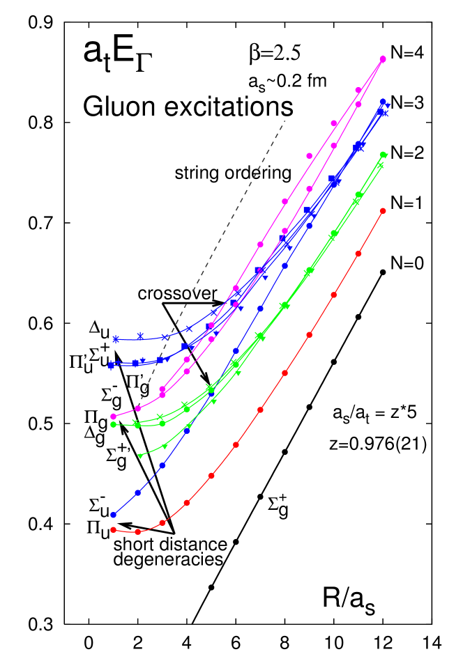
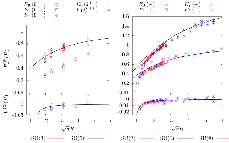
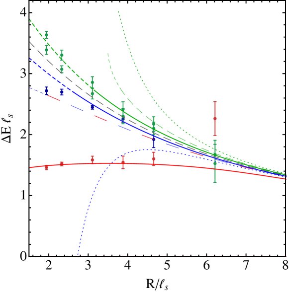
Since the first studies concerning open flux tubes in the early 80‘s [22, 23, 24, 25, 26, 27] the accuracy and reliability of lattice measurements [67, 68, 69, 70, 71, 72, 73, 74, 75, 76, 77, 78, 79, 80, 81, 82, 83, 84, 85, 86, 87, 88, 89, 90, 31, 91, 92, 93, 94, 95, 96] in 3 and 4D SU($N$) gauge theories has steadily improved, together with much better control over systematic uncertainties. High accuracy measurements of large loops have become available by the introduction of the multilevel algorithm [101], which has since been used extensively for studies of open flux tube spectra [102, 103, 104, 105, 106, 107, 108, 109, 110, 111, 112, 113]. Similar studies have also been performed in 3D U(1) [114, 62] and 3D Z₂ [115, 116, 117, 118, 119, 120, 42] gauge theories. Measurement of the energy levels of closed flux tubes have started only little later [121, 122, 123, 124, 125, 126, 127, 128, 129, 130, 131, 132, 133, 134]. We show a collection of results for the lowest energy levels of open and closed flux tubes in figures 1 and 2, respectively.

Figure 1: Right: Results for the spectrum of the open flux tube in 4D SU(3) gauge theory from 92. States are labeled by the projection of angular momentum $J$ on the string axis ($\Sigma,\Pi,\Delta$ for $J=0,1,2$), parity $P$ (subscripts $g,u$ for 1,-1) and charge conjugation $C$ (superscript +,-). The study used anisotropic lattices with lattice spacings $a_{s}$ (spatial) and $a_{t}$ (temporal). Left: Results for the spectrum of the open flux tube in 3D SU($N=2,3,5$) gauge theories from 111, 113, 135 ($\beta=5.0,\,20.0$ and 54.0, respectively) and SU(2) from 106, 109 (gray symbols; $\beta=7.5$) versus $\sqrt{\sigma}R$. We have rescaled the energies such that the leading order expansion of the LC energy levels is equal to $n$ (see 111). The states are classified according to $(CP)$. The lower panel shows a blow-up of the groundstate energies. The solid lines correspond to the LC spectrum.

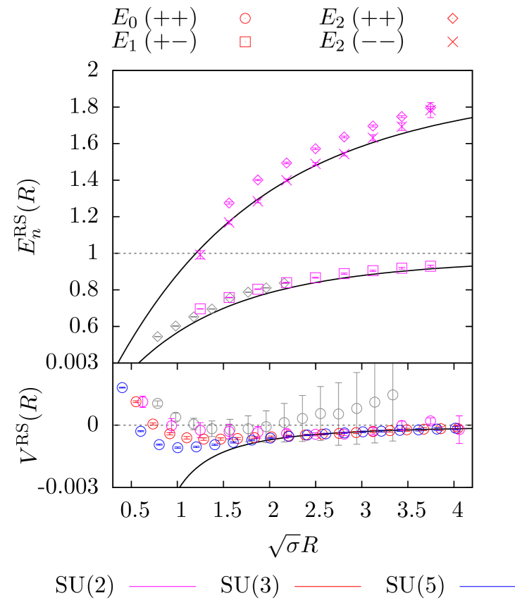
To briefly summarize the main findings: For (most of) the energy levels the data shows a remarkable agreement with the full LC predictions down to small values of $\sqrt{\sigma}R\sim 1$, rather than with its expansion in powers of $R^{-1}$, independently of the number of dimensions and the gauge group.[56] Typically, agreement with the string states is seen starting from $R\approx 0.5$ fm for the groundstate up to 2 fm for the excited states, increasing with the excitation level. The convergence to the LC spectrum appears to be enhanced when going to larger values of $N$. These observations are in full agreement with the discussion of the EST in sec. 2 and 3 and are basically independent of the lattice spacing and thus should hold in the continuum. With ever increasing accuracy, deviations from the LC spectrum become visible, once more in agreement with the EST. Some of those deviations in 4D SU($N$) gauge theories, however, are not in agreement with the the spectrum in eq. (7) and could be signs for the expected massive modes on the flux tube.

Figure 2: As figure 1 (right) for the energy levels of the closed flux tube in 4D SU($N=3,5$) (left), $\beta=6.0625$ and $17.63$, and 3D SU($N=2,6,8$) (right) ($\beta=16,171$ and $306$) gauge theories from [132, 134] versus $\sqrt{\sigma}R$. We have included states with $q=0$, set $n=(N_{L}+N_{R})/2$ and rescaled the energies as in figure 1. The states in 4D are classified by $(J^{CP})$ and in 3D by $(P)$.

4.1.2 Corrections to the LC spectrum for open strings

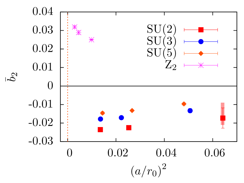
Concerning the comparison between lattice results and the EST, the open string channel is advantageous because the first correction not fixed in terms of the string tension is of $O(R^{-4})$ (compared to $O(R^{-7})$ for closed strings) and only depends on one free parameter $\bar{b}_{2}=\sqrt{\sigma^{3}}b_{2}$. The comparison to the boundary corrections is conveniently done in the 3D case and the associated coefficient $\bar{b}_{2}$ has first been extracted from the excited states in SU(2) gauge theories [111] and later from the groundstate in Z₂ [42] and in SU($N$) gauge theories for $N=2,3$ [113] ($N=4,5,6$ are in preparation [135]) at several lattice spacings. Including the boundary correction, the EST can describe the groundstate data down to about 0.4 fm and is in qualitative agreement with the excited states [111, 42]. In fact, by leaving the exponent of the correction term free, it can be shown that it takes a value of 4 down to $R\approx 0.4$ fm [135]. In figure 3, we collect the results for $\bar{b}_{2}$ versus the squared lattice spacing. The plot illustrates the non-universality of $\bar{b}_{2}$. Interestingly, it appears to become larger with increasing $N$, possibly tending towards zero for $N\to\infty$, and is positive for Z₂ gauge theory, where, however, $\bar{b}_{2}$ does not show a perfect scaling towards the continuum. From the open string groundstate in 3D U(1) gauge theory, also the rigidity contribution was extracted[62], thanks to an enhancement of $\alpha$ towards the continuum. This is not expected for SU($N$) and indeed, a positive deviation from the LC spectrum is visible for short strings, while the rigidity term gives a negative Coulomb-like contribution at small values of $\sqrt{\sigma/\alpha}R$.[60]

Figure 3: Left: Results for the boundary coefficient $\bar{b}_{2}$ obtained from the groundstate energies for $N=2$ and 3 [113, 135], preliminary results for $N=5$ [135], and results from Z₂ gauge theory [42]. The red band is the result for SU(2) extracted from excited states [111]. Right: Comparison of the energy differences to the groundstate of the closed flux tubes in 4D SU(3) from [132], with the predictions from TBA (solid lines), including the worldsheet axion, taken from [55]. Scalar, pseudoscalar and spin 2 states are shown in blue, red and green, respectively. The dashed lines correspond to the EST prediction from TBA without the axion, the dashed gray line is the LC prediction and the dotted lines are the LO and NLO orders in the $R^{-1}$ expansion. Here $\ell_{s}=\sqrt{\sigma}^{-1}$.

In 4D, such an analysis is still missing. The spectrum [91, 92, 94] shows a strong rearrangement of energy levels from short distance [93] to long distance (string) degeneracies. The spectrum graduates in states that show a fast convergence to the string states and those with an anomalously slow approach, such as the $\Sigma_{u}^{-}$ ($J^{CP}=0^{--}$) state and possibly also the states ${\Sigma^{\prime}}_{g}^{-}$ and $\Sigma_{g}^{-}$ (similar states have been found for closed flux tubes), which possibly receive contributions from massive modes [95, 132, 55, 56]. Note, that the 4D energies from Morningstar:1998da,Juge:2002br,Juge:2004xr typically overshoot the LC predictions in the large $R$ limit, which could be a sign for contaminations from excited states (e.g. Majumdar:2002mr,Brandt:2010bw,Athenodorou:2010cs) and a continuum limit is still missing.

4.1.3 Corrections to the LC spectrum for closed strings

For closed flux tubes, the corrections to the LC spectrum for the groundstate and excited states in 3D start at $O(R^{-7})$ and are thus harder to detect. Interestingly, all of them appear to be negative, in contrast to the positive corrections in the open case. For 4D the correction to excited states is universal and of $O(R^{-5})$. There is one state with $J^{P}=0^{-}$, which deviates from the string energy levels and thus qualifies as a massive excitation. Leaving this state aside, an analysis of the corrections to the LC energy levels, has been performed for 4D [132] (mostly for $N=3$) and 3D [133, 134] (for $N=2,3,4,5,6$ and 8). For the groundstate, the results in general show good agreement with the EST predictions, leading to an exponent of -7 or -9 (at most -5) for the corrections to the LC spectrum with $N\geq 3$.

For the excited states in 3D a simple $R^{-7}$ correction is basically ruled out when fitting the data down to $R\sqrt{\sigma}\approx 4.5-5.0$ [133]. It is likely that the radius of convergence, $R_{C}$, of the derivative expansion in the full EST increases with the excitation level (similar to the one of the LC spectrum). An analysis with an heuristic resummed correction[133] yields $R_{C}$ of the order of $R_{C}$ of the LC spectrum. The TBA analysis, which corresponds to a more convergent expansion, obtains good fits and possibly some hints of a massive resonance.[56] For 4D, a simple $R^{-5}$ correction down to $R_{C}$ of the LC spectrum is not ruled out. Nonetheless, a similar increase of the deviations to the LC spectrum are seen with increasing excitation level. For closed flux tubes there are also states with non-zero longitudinal momentum, $q\neq 0$. The lattice results for those states agree with the above findings and basically consistent with the LC predictions. [132, 133, 134]

Looking at the state with $J^{P}=0^{-}$, both a simple heuristic analysis,[132] and the TBA method,[55, 56] show agreement of the data with a massive mode contribution. In particular, the latter explicitly identifies the worldsheet axion and shows excellent agreement with this state and the next excited state in this channel. The $0^{-}$ state with $q=1$ shows the same behaviour as the associated $q=0$ state. However, the next excited state in the $q=1$, $0^{-}$-channel behaves differently, basically following the LC predictions. It would be interesting to see whether the TBA analysis can explain the behaviour of this state, too.

Figure 4: Left: Flux tube profile at the midpoint in 3D SU(2) from 136 for $R\approx 1.4$ fm. The $y$ axis shows the expectation value of the Polyakov loop correlator in $x_{1}$ direction correlated with a plaquette in $(x_{1},x_{2})$ direction versus the transverse displacement in lattice units ($a\approx 0.07$ fm). The solid line is a fit to a Gaussian with correction terms (see eq. (20) in 136). Right: Flux tube width versus its length in lattice units, again from 136, including a logarithmic fit.

4.2 Width of the flux tube

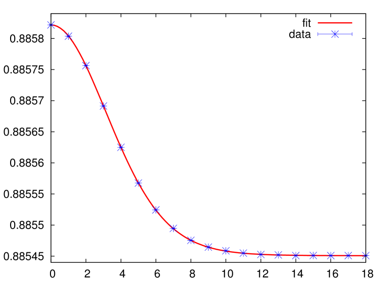
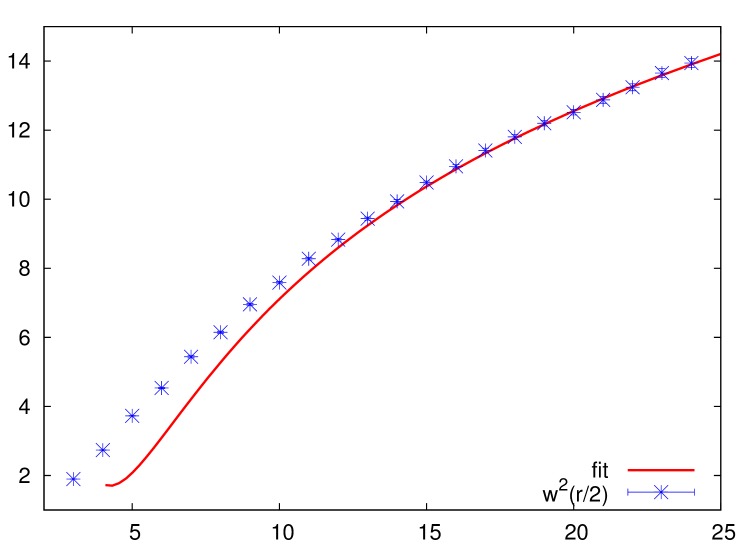
Another observable to investigate the range of validity of the EST is the flux tube profile. Studies of the profile have been performed in SU($N$) [137, 138, 139, 140, 141, 142, 143, 144, 145, 146, 86, 147, 148, 149, 150, 151, 152, 153, 154, 155, 156, 157, 158, 159, 160, 161, 136, 162, 163, 164], U(1) [165, 166, 104, 167] and Z₂ [168, 63] gauge theories and confirmed the formation of a tube-like object. Most studies have compared the profile to the predictions from the dual-superconductor model only, whose discussion is beyond the scope of this review. Initial studies [140, 141, 142] comparing to the EST, saw agreement starting from around $R\approx 0.8$ fm [86], yet, without being able to clearly identify the logarithmic broadening with increasing $R$. The latter has first been confirmed in Z₂ gauge theory [168, 63]. Similar studies in 3D SU(2) [136] and U(1) [167] and 4D SU(3) gauge theory [163] only became available recently. These studies show the logarithmic broadening of the string with $R$ and evidence for the Gaussian shape for flux tubes with $R\gtrsim 1.3$ fm. Higher orders could potentially increase the range of agreement. The results for the profile, including a Gaussian fit with EST inspired corrections [66], and the width from Gliozzi:2010zv, together with a logarithmic fit, are shown in figure 4. The study from Cardoso:2013lla focuses on 4D SU(3) and has gone the next step, trying to identify signs of a mixture of the vortex and string pictures in the profile. They fitted the profile to a convolution of a Gaussian with an exponential decrease and found a good description of the data for distances between 0.4 and 1.4 fm. The associated penetration length remains constant (at 0.22 fm) with $R$, in agreement with the dual superconductor picture, while the squared width increases logarithmically. Note, that both studies still lack a continuum extrapolation. In 3D U(1) [167], the width increases logarithmically, but the tail of the profile does not show a Gaussian shape. It would be interesting to see whether a combined vortex/string analysis also works for this high precision case.

5 Summary and perspectives

In this review, we have summarized the current knowledge about the theoretical foundation of EST for confining flux tubes and the associated predictions, together with comparisons to simulations in lattice QCD. In sec. 2 and 3, we have accumulated the new theoretical insights of the last few years in a homogeneous presentation of the EST. As shown in sec. 4, on one hand predicted deviations from the LC spectrum are in good agreement with lattice results. On the other hand, the TBA approach has allowed a solid interpretation of anomalous data in 4D in terms of a massive pseudoscalar mode. For the width of the flux tube, simulations show good agreement with the EST predictions starting from around 1 to 1.3 fm.

Despite the good agreement, there are several open questions. To begin with, it would be interesting to improve on the precision for the excited states in 3D and to reliably perform the analyses concerning corrections to the spectrum for 4D. In particular, the contribution of the axion to the open string spectrum has not been computed and a general understanding of other possible massive modes is lacking. Concerning the profile, the competition between the exponential and the Gaussian tail highlights the need for more theoretical control over the simple idea of the flux tube as a vortex with stringy fluctuations on top. [163]. One more ripple in the consolidated understanding of the EST is provided by the contribution of the rigidity term to the observables, which accounts for some features of the spectrum in U(1) gauge theory and may appear in other gauge theories, too. It is crucial to confirm these effects via an explicitly Lorentz invariant computation. On a more speculative level, the availability of first principle computations of the effective action in holographic setup[29, 169, 170, 171, 172] fuels the hope that one might, in turn, extract from the data useful information about the holographic dual of Yang-Mills theories. Finally, it would be interesting to gain more insight about modifications coming from the finite masses of ‘static’ quarks and the presence of sea quarks.

There are some issues related to flux tubes and the EST that we could not discuss due to length constraints. This concerns signatures of the EST at finite temperature [173, 174, 175] and the behaviour of the width in this regime [176, 177, 178, 179]. One can also study flux tubes in different representations [180, 181, 134], so called $k$-strings, baryonic boundstates [182, 183, 184] or the interface free energy in 3D Z2 gauge theory [185, 186]. These studies typically observe rather good agreement with the EST and massive modes have also been observed for $k$-strings [181, 134]. There are also other aspects of the potential which have not been discussed (see Greensite:2003bk,Bali:2000gf, for instance).

Acknowledgements

We acknowledge very enlightening discussions and correspondence with A. Athenodorou, M. Caselle, F. Cuteri, R. Flauger, D. Gaiotto, P. Majumdar and M. Panero. Research at Perimeter Institute is supported by the Government of Canada through Industry Canada and by the Province of Ontario through the Ministry of Research & Innovation. BB receives funding by the DFG via SFB/TRR 55 and the Emmy Noether Programme EN 1064/2-1.

References

- [1] J. Greensite, Prog. Part. Nucl. Phys. 51, 1 (2003), arXiv:hep-lat/0301023 [hep-lat], 10.1016/S0146-6410(03)90012-3.
- [2] G. S. Bali, Phys. Rept. 343, 1 (2001), arXiv:hep-ph/0001312 [hep-ph], 10.1016/S0370-1573(00)00079-X.
- [3] T. Goto, Prog. Theor. Phys. 46, 1560 (1971), 10.1143/PTP.46.1560.
- [4] P. Goddard, J. Goldstone, C. Rebbi and C. B. Thorn, Nucl. Phys. B56, 109 (1973), 10.1016/0550-3213(73)90223-X.
- [5] K. G. Wilson, Phys. Rev. D10, 2445 (1974), 10.1103/PhysRevD.10.2445, [,45(1974)].
- [6] J. B. Kogut and L. Susskind, Phys. Rev. D11, 395 (1975), 10.1103/PhysRevD.11.395.
- [7] N. Isgur and J. E. Paton, Phys. Rev. D31, 2910 (1985), 10.1103/PhysRevD.31.2910.
- [8] Y. Nambu, Phys. Lett. B80, 372 (1979), 10.1016/0370-2693(79)91193-6.
- [9] M. Luscher, K. Symanzik and P. Weisz, Nucl. Phys. B173, 365 (1980), 10.1016/0550-3213(80)90009-7.
- [10] A. M. Polyakov, Nucl. Phys. B164, 171 (1980), 10.1016/0550-3213(80)90507-6.
- [11] M. Baker, J. S. Ball and F. Zachariasen, Phys. Rept. 209, 73 (1991), 10.1016/0370-1573(91)90123-4.
- [12] H. B. Nielsen and P. Olesen, Nucl. Phys. B61, 45 (1973), 10.1016/0550-3213(73)90350-7.
- [13] Y. Nambu, Phys. Rev. D10, 4262 (1974), 10.1103/PhysRevD.10.4262.
- [14] S. Mandelstam, Phys. Rept. 23, 245 (1976), 10.1016/0370-1573(76)90043-0.
- [15] G. ’t Hooft, Nucl. Phys. B153, 141 (1979), 10.1016/0550-3213(79)90595-9.
- [16] M. Luscher, G. Munster and P. Weisz, Nucl. Phys. B180, 1 (1981), 10.1016/0550-3213(81)90151-6.
- [17] M. Luscher, Nucl. Phys. B180, 317 (1981), 10.1016/0550-3213(81)90423-5.
- [18] M. Luscher and P. Weisz, JHEP 07, 014 (2004), arXiv:hep-th/0406205 [hep-th], 10.1088/1126-6708/2004/07/014.
- [19] J. Polchinski and A. Strominger, Phys. Rev. Lett. 67, 1681 (1991), 10.1103/PhysRevLett.67.1681.
- [20] S. Dubovsky, R. Flauger and V. Gorbenko, JHEP 09, 044 (2012), arXiv:1203.1054 [hep-th], 10.1007/JHEP09(2012)044.
- [21] O. Aharony and Z. Komargodski, JHEP 05, 118 (2013), arXiv:1302.6257 [hep-th], 10.1007/JHEP05(2013)118.
- [22] C. B. Lang and C. Rebbi, Phys. Lett. B115, 137 (1982), 10.1016/0370-2693(82)90813-9, [,322(1982)].
- [23] L. A. Griffiths, C. Michael and P. E. L. Rakow, Phys. Lett. B129, 351 (1983), 10.1016/0370-2693(83)90680-9.
- [24] J. D. Stack, Phys. Rev. D29, 1213 (1984), 10.1103/PhysRevD.29.1213.
- [25] N. A. Campbell, C. Michael and P. E. L. Rakow, Phys. Lett. B139, 288 (1984), 10.1016/0370-2693(84)91082-7.
- [26] N. A. Campbell, L. A. Griffiths, C. Michael and P. E. L. Rakow, Phys. Lett. B142, 291 (1984), 10.1016/0370-2693(84)91200-0.
- [27] P. de Forcrand, G. Schierholz, H. Schneider and M. Teper, Phys. Lett. B160, 137 (1985), 10.1016/0370-2693(85)91480-7.
- [28] E. T. Akhmedov, M. N. Chernodub, M. I. Polikarpov and M. A. Zubkov, Phys. Rev. D53, 2087 (1996), arXiv:hep-th/9505070 [hep-th], 10.1103/PhysRevD.53.2087.
- [29] O. Aharony and E. Karzbrun, JHEP 06, 012 (2009), arXiv:0903.1927 [hep-th], 10.1088/1126-6708/2009/06/012.
- [30] O. Aharony and M. Field, JHEP 01, 065 (2011), arXiv:1008.2636 [hep-th], 10.1007/JHEP01(2011)065.
- [31] S. Necco and R. Sommer, Nucl. Phys. B622, 328 (2002), arXiv:hep-lat/0108008 [hep-lat], 10.1016/S0550-3213(01)00582-X.
- [32] I. Low and A. V. Manohar, Phys. Rev. Lett. 88, 101602 (2002), arXiv:hep-th/0110285 [hep-th], 10.1103/PhysRevLett.88.101602.
- [33] J. D. Cohn and V. Periwal, Nucl. Phys. B395, 119 (1993), arXiv:hep-th/9205026 [hep-th], 10.1016/0550-3213(93)90210-G.
- [34] H. B. Meyer, JHEP 05, 066 (2006), arXiv:hep-th/0602281 [hep-th], 10.1088/1126-6708/2006/05/066.
- [35] S. R. Coleman, J. Wess and B. Zumino, Phys. Rev. 177, 2239 (1969), 10.1103/PhysRev.177.2239.
- [36] C. G. Callan, Jr., S. R. Coleman, J. Wess and B. Zumino, Phys. Rev. 177, 2247 (1969), 10.1103/PhysRev.177.2247.
- [37] D. V. Volkov, Fiz. Elem. Chast. Atom. Yadra 4, 3 (1973).
- [38] O. Aharony and M. Dodelson, JHEP 02, 008 (2012), arXiv:1111.5758 [hep-th], 10.1007/JHEP02(2012)008.
- [39] F. Gliozzi and M. Meineri, JHEP 08, 056 (2012), arXiv:1207.2912 [hep-th], 10.1007/JHEP08(2012)056.
- [40] P. Cooper, Phys. Rev. D88, 025047 (2013), arXiv:1303.0743 [hep-th], 10.1103/PhysRevD.88.025047.
- [41] J. Gomis, K. Kamimura and J. M. Pons, Nucl. Phys. B871, 420 (2013), arXiv:1205.1385 [hep-th], 10.1016/j.nuclphysb.2013.02.018.
- [42] M. Billo, M. Caselle, F. Gliozzi, M. Meineri and R. Pellegrini, JHEP 05, 130 (2012), arXiv:1202.1984 [hep-th], 10.1007/JHEP05(2012)130.
- [43] L. Mezincescu and P. K. Townsend, Phys. Rev. Lett. 105, 191601 (2010), arXiv:1008.2334 [hep-th], 10.1103/PhysRevLett.105.191601.
- [44] J. F. Arvis, Phys. Lett. B127, 106 (1983), 10.1016/0370-2693(83)91640-4.
- [45] J. Polchinski, String theory. Vol. 1: An introduction to the bosonic string (Cambridge University Press, 2007).
- [46] N. D. Hari Dass and P. Matlock, Indian J. Phys. 88, 965 (2014), arXiv:0709.1765 [hep-th], 10.1007/s12648-014-0493-7.
- [47] M. Natsuume, Phys. Rev. D48, 835 (1993), arXiv:hep-th/9206062 [hep-th], 10.1103/PhysRevD.48.835.
- [48] A. M. Polyakov, Phys. Lett. B103, 207 (1981), 10.1016/0370-2693(81)90743-7.
- [49] S. Hellerman, S. Maeda, J. Maltz and I. Swanson, JHEP 09, 183 (2014), arXiv:1405.6197 [hep-th], 10.1007/JHEP09(2014)183.
- [50] O. Aharony, M. Field and N. Klinghoffer, JHEP 04, 048 (2012), arXiv:1111.5757 [hep-th], 10.1007/JHEP04(2012)048.
- [51] O. Aharony and N. Klinghoffer, JHEP 12, 058 (2010), arXiv:1008.2648 [hep-th], 10.1007/JHEP12(2010)058.
- [52] J. M. Drummond (2004), arXiv:hep-th/0411017 [hep-th].
- [53] N. D. Hari Dass and P. Matlock (2006), arXiv:hep-th/0606265 [hep-th].
- [54] S. Dubovsky, R. Flauger and V. Gorbenko, JHEP 09, 133 (2012), arXiv:1205.6805 [hep-th], 10.1007/JHEP09(2012)133.
- [55] S. Dubovsky, R. Flauger and V. Gorbenko, Phys. Rev. Lett. 111, 062006 (2013), arXiv:1301.2325 [hep-th], 10.1103/PhysRevLett.111.062006.
- [56] S. Dubovsky, R. Flauger and V. Gorbenko, J. Exp. Theor. Phys. 120, 399 (2015), arXiv:1404.0037 [hep-th], 10.1134/S1063776115030188.
- [57] M. Caselle, D. Fioravanti, F. Gliozzi and R. Tateo, JHEP 07, 071 (2013), arXiv:1305.1278 [hep-th], 10.1007/JHEP07(2013)071.
- [58] S. Dubovsky and V. Gorbenko (2015), arXiv:1511.01908 [hep-th].
- [59] A. M. Polyakov, Nucl. Phys. B268, 406 (1986), 10.1016/0550-3213(86)90162-8.
- [60] G. German and H. Kleinert, Phys. Rev. D40, 1108 (1989), 10.1103/PhysRevD.40.1108.
- [61] J. Ambjørn, Y. Makeenko and A. Sedrakyan, Phys. Rev. D89, 106010 (2014), arXiv:1403.0893 [hep-th], 10.1103/PhysRevD.89.106010.
- [62] M. Caselle, M. Panero, R. Pellegrini and D. Vadacchino, JHEP 01, 105 (2015), arXiv:1406.5127 [hep-lat], 10.1007/JHEP01(2015)105.
- [63] M. Caselle, F. Gliozzi, U. Magnea and S. Vinti, Nucl. Phys. B460, 397 (1996), arXiv:hep-lat/9510019 [hep-lat], 10.1016/0550-3213(95)00639-7.
- [64] N. D. Mermin and H. Wagner, Phys. Rev. Lett. 17, 1133 (1966), 10.1103/PhysRevLett.17.1133.
- [65] S. R. Coleman, Commun. Math. Phys. 31, 259 (1973), 10.1007/BF01646487.
- [66] F. Gliozzi, M. Pepe and U. J. Wiese, JHEP 11, 053 (2010), arXiv:1006.2252 [hep-lat], 10.1007/JHEP11(2010)053.
- [67] S. W. Otto and J. D. Stack, Phys. Rev. Lett. 52, 2328 (1984), 10.1103/PhysRevLett.52.2328.
- [68] A. Hasenfratz, P. Hasenfratz, U. M. Heller and F. Karsch, Z. Phys. C25, 191 (1984), 10.1007/BF01557479.
- [69] D. Barkai, K. J. M. Moriarty and C. Rebbi, Phys. Rev. D30, 1293 (1984), 10.1103/PhysRevD.30.1293.
- [70] J. Ambjorn, P. Olesen and C. Peterson, Nucl. Phys. B244, 262 (1984), 10.1016/0550-3213(84)90193-7.
- [71] R. Sommer and K. Schilling, Z. Phys. C29, 95 (1985), 10.1007/BF01571386.
- [72] A. Huntley and C. Michael, Nucl. Phys. B270, 123 (1986), 10.1016/0550-3213(86)90548-1.
- [73] F. Gutbrod, Z. Phys. C30, 585 (1986), 10.1007/BF01571807.
- [74] S. Itoh, Y. Iwasaki, Y. Oyanagi and T. Yoshie, Nucl. Phys. B274, 33 (1986), 10.1016/0550-3213(86)90616-4.
- [75] M. Flensburg, A. Irback and C. Peterson, Z. Phys. C36, 629 (1987), 10.1007/BF01630599.
- [76] N. A. Campbell, A. Huntley and C. Michael, Nucl. Phys. B306, 51 (1988), 10.1016/0550-3213(88)90170-8.
- [77] J. Hoek, Z. Phys. C35, 369 (1987), 10.1007/BF01570774.
- [78] I. J. Ford, R. H. Dalitz and J. Hoek, Phys. Lett. B208, 286 (1988), 10.1016/0370-2693(88)90431-5.
- [79] S. Perantonis, A. Huntley and C. Michael, Nucl. Phys. B326, 544 (1989), 10.1016/0550-3213(89)90141-7.
- [80] R. D. Mawhinney, Phys. Rev. D41, 3209 (1990), 10.1103/PhysRevD.41.3209.
- [81] S. Perantonis and C. Michael, Nucl. Phys. B347, 854 (1990), 10.1016/0550-3213(90)90386-R.
- [82] C. Michael and S. J. Perantonis, J. Phys. G18, 1725 (1992), 10.1088/0954-3899/18/11/005.
- [83] UKQCD Collaboration (S. P. Booth, D. S. Henty, A. Hulsebos, A. C. Irving, C. Michael and P. W. Stephenson), Phys. Lett. B294, 385 (1992), arXiv:hep-lat/9209008 [hep-lat], 10.1016/0370-2693(92)91538-K.
- [84] G. S. Bali and K. Schilling, Phys. Rev. D46, 2636 (1992), 10.1103/PhysRevD.46.2636.
- [85] G. S. Bali and K. Schilling, Phys. Rev. D47, 661 (1993), arXiv:hep-lat/9208028 [hep-lat], 10.1103/PhysRevD.47.661.
- [86] G. S. Bali, K. Schilling and C. Schlichter, Phys. Rev. D51, 5165 (1995), arXiv:hep-lat/9409005 [hep-lat], 10.1103/PhysRevD.51.5165.
- [87] Y. Iwasaki, K. Kanaya, T. Kaneko and T. Yoshie, Phys. Rev. D56, 151 (1997), arXiv:hep-lat/9610023 [hep-lat], 10.1103/PhysRevD.56.151.
- [88] G. S. Bali, K. Schilling and A. Wachter, Phys. Rev. D56, 2566 (1997), arXiv:hep-lat/9703019 [hep-lat], 10.1103/PhysRevD.56.2566.
- [89] B. Beinlich, F. Karsch, E. Laermann and A. Peikert, Eur. Phys. J. C6, 133 (1999), arXiv:hep-lat/9707023 [hep-lat], 10.1007/s100520050326.
- [90] R. G. Edwards, U. M. Heller and T. R. Klassen, Nucl. Phys. B517, 377 (1998), arXiv:hep-lat/9711003 [hep-lat], 10.1016/S0550-3213(98)80003-5.
- [91] C. J. Morningstar, K. J. Juge and J. Kuti, Nucl. Phys. Proc. Suppl. 73, 590 (1999), arXiv:hep-lat/9809098 [hep-lat], 10.1016/S0920-5632(99)85147-0.
- [92] K. J. Juge, J. Kuti and C. Morningstar, Phys. Rev. Lett. 90, 161601 (2003), arXiv:hep-lat/0207004 [hep-lat], 10.1103/PhysRevLett.90.161601.
- [93] G. S. Bali and A. Pineda, Phys. Rev. D69, 094001 (2004), arXiv:hep-ph/0310130 [hep-ph], 10.1103/PhysRevD.69.094001.
- [94] K. J. Juge, J. Kuti and C. Morningstar, QCD string formation and the Casimir energy, in Color confinement and hadrons in quantum chromodynamics. Proceedings, International Conference, Confinement 2003, Wako, Japan, July 21-24, 2003, (2004), pp. 233–248. arXiv:hep-lat/0401032 [hep-lat].
- [95] J. Kuti, PoS LAT2005, 001 (2006), arXiv:hep-lat/0511023 [hep-lat], [PoSJHW2005,009(2006)].
- [96] R. Lohmayer and H. Neuberger, JHEP 08, 102 (2012), arXiv:1206.4015 [hep-lat], 10.1007/JHEP08(2012)102.
- [97] M. Falcioni, M. L. Paciello, G. Parisi and B. Taglienti, Nucl. Phys. B251, 624 (1985), 10.1016/0550-3213(85)90280-9.
- [98] A. Hasenfratz and F. Knechtli, Phys. Rev. D64, 034504 (2001), arXiv:hep-lat/0103029 [hep-lat], 10.1103/PhysRevD.64.034504.
- [99] C. Michael and I. Teasdale, Nucl. Phys. B215, 433 (1983), 10.1016/0550-3213(83)90674-0.
- [100] B. Blossier, M. Della Morte, G. von Hippel, T. Mendes and R. Sommer, JHEP 04, 094 (2009), arXiv:0902.1265 [hep-lat], 10.1088/1126-6708/2009/04/094.
- [101] M. Luscher and P. Weisz, JHEP 09, 010 (2001), arXiv:hep-lat/0108014 [hep-lat], 10.1088/1126-6708/2001/09/010.
- [102] M. Luscher and P. Weisz, JHEP 07, 049 (2002), arXiv:hep-lat/0207003 [hep-lat], 10.1088/1126-6708/2002/07/049.
- [103] P. Majumdar, Nucl. Phys. B664, 213 (2003), arXiv:hep-lat/0211038 [hep-lat], 10.1016/S0550-3213(03)00447-4.
- [104] Y. Koma, M. Koma and P. Majumdar, Nucl. Phys. B692, 209 (2004), arXiv:hep-lat/0311016 [hep-lat], 10.1016/j.nuclphysb.2004.05.024.
- [105] M. Caselle, M. Pepe and A. Rago, JHEP 10, 005 (2004), arXiv:hep-lat/0406008 [hep-lat], 10.1088/1126-6708/2004/10/005.
- [106] P. Majumdar (2004), arXiv:hep-lat/0406037 [hep-lat].
- [107] H. B. Meyer, Nucl. Phys. B758, 204 (2006), arXiv:hep-lat/0607015 [hep-lat], 10.1016/j.nuclphysb.2006.09.027.
- [108] N. D. Hari Dass and P. Majumdar, JHEP 10, 020 (2006), arXiv:hep-lat/0608024 [hep-lat], 10.1088/1126-6708/2006/10/020.
- [109] N. D. Hari Dass and P. Majumdar, Phys. Lett. B658, 273 (2008), arXiv:hep-lat/0702019 [HEP-LAT], 10.1016/j.physletb.2007.08.097.
- [110] B. B. Brandt and P. Majumdar, Phys. Lett. B682, 253 (2009), arXiv:0905.4195 [hep-lat], 10.1016/j.physletb.2009.11.010.
- [111] B. B. Brandt, JHEP 02, 040 (2011), arXiv:1010.3625 [hep-lat], 10.1007/JHEP02(2011)040.
- [112] A. Mykkanen, JHEP 12, 069 (2012), arXiv:1209.2372 [hep-lat], 10.1007/JHEP12(2012)069.
- [113] B. B. Brandt, PoS EPS-HEP2013, 540 (2013), arXiv:1308.4993 [hep-lat].
- [114] M. Panero, Nucl. Phys. Proc. Suppl. 140, 665 (2005), arXiv:hep-lat/0408002 [hep-lat], 10.1016/j.nuclphysbps.2004.11.203, [,665(2004)].
- [115] M. Caselle, R. Fiore, F. Gliozzi, M. Hasenbusch and P. Provero, Nucl. Phys. B486, 245 (1997), arXiv:hep-lat/9609041 [hep-lat], 10.1016/S0550-3213(96)00672-4.
- [116] M. Caselle, M. Hasenbusch and M. Panero, JHEP 01, 057 (2003), arXiv:hep-lat/0211012 [hep-lat], 10.1088/1126-6708/2003/01/057.
- [117] M. Caselle, M. Hasenbusch and M. Panero, JHEP 05, 032 (2004), arXiv:hep-lat/0403004 [hep-lat], 10.1088/1126-6708/2004/05/032.
- [118] M. Caselle, M. Hasenbusch and M. Panero, JHEP 01, 076 (2006), arXiv:hep-lat/0510107 [hep-lat], 10.1088/1126-6708/2006/01/076.
- [119] M. Caselle and M. Zago, Eur. Phys. J. C71, 1658 (2011), arXiv:1012.1254 [hep-lat], 10.1140/epjc/s10052-011-1658-6.
- [120] M. Billo, M. Caselle and R. Pellegrini, JHEP 01, 104 (2012), arXiv:1107.4356 [hep-th], 10.1007/JHEP01(2012)104, 10.1007/JHEP04(2013)097, [Erratum: JHEP04,097(2013)].
- [121] C. Michael, J. Phys. G13, 1001 (1987), 10.1088/0305-4616/13/8/007.
- [122] C. Michael, G. A. Tickle and M. J. Teper, Phys. Lett. B207, 313 (1988), 10.1016/0370-2693(88)90582-5.
- [123] C. Michael, Phys. Lett. B232, 247 (1989), 10.1016/0370-2693(89)91695-X.
- [124] M. Teper, Phys. Lett. B311, 223 (1993), 10.1016/0370-2693(93)90559-Z.
- [125] UKQCD Collaboration (C. Michael and P. W. Stephenson), Phys. Rev. D50, 4634 (1994), arXiv:hep-lat/9403004 [hep-lat], 10.1103/PhysRevD.50.4634.
- [126] M. J. Teper, Phys. Rev. D59, 014512 (1999), arXiv:hep-lat/9804008 [hep-lat], 10.1103/PhysRevD.59.014512.
- [127] B. Lucini and M. Teper, JHEP 06, 050 (2001), arXiv:hep-lat/0103027 [hep-lat], 10.1088/1126-6708/2001/06/050.
- [128] B. Lucini and M. Teper, Phys. Rev. D64, 105019 (2001), arXiv:hep-lat/0107007 [hep-lat], 10.1103/PhysRevD.64.105019.
- [129] B. Lucini and M. Teper, Phys. Rev. D66, 097502 (2002), arXiv:hep-lat/0206027 [hep-lat], 10.1103/PhysRevD.66.097502.
- [130] K. J. Juge, J. Kuti, F. Maresca, C. Morningstar and M. J. Peardon, Nucl. Phys. Proc. Suppl. 129, 703 (2004), arXiv:hep-lat/0309180 [hep-lat], 10.1016/S0920-5632(03)02686-0, [,703(2003)].
- [131] A. Athenodorou, B. Bringoltz and M. Teper, Phys. Lett. B656, 132 (2007), arXiv:0709.0693 [hep-lat], 10.1016/j.physletb.2007.09.045.
- [132] A. Athenodorou, B. Bringoltz and M. Teper, JHEP 02, 030 (2011), arXiv:1007.4720 [hep-lat], 10.1007/JHEP02(2011)030.
- [133] A. Athenodorou, B. Bringoltz and M. Teper, JHEP 05, 042 (2011), arXiv:1103.5854 [hep-lat], 10.1007/JHEP05(2011)042.
- [134] A. Athenodorou and M. Teper (2016), arXiv:1602.07634 [hep-lat].
- [135] B. B. Brandt, in preparation (2016).
- [136] F. Gliozzi, M. Pepe and U. J. Wiese, Phys. Rev. Lett. 104, 232001 (2010), arXiv:1002.4888 [hep-lat], 10.1103/PhysRevLett.104.232001.
- [137] M. Fukugita and T. Niuya, Phys. Lett. B132, 374 (1983), 10.1016/0370-2693(83)90329-5.
- [138] J. W. Flower and S. W. Otto, Phys. Lett. B160, 128 (1985), 10.1016/0370-2693(85)91478-9.
- [139] J. Wosiek and R. W. Haymaker, Phys. Rev. D36, 3297 (1987), 10.1103/PhysRevD.36.3297.
- [140] R. Sommer, Nucl. Phys. B291, 673 (1987), 10.1016/0550-3213(87)90490-1.
- [141] A. Di Giacomo, M. Maggiore and S. Olejnik, Phys. Lett. B236, 199 (1990), 10.1016/0370-2693(90)90828-T.
- [142] A. Di Giacomo, M. Maggiore and S. Olejnik, Nucl. Phys. B347, 441 (1990), 10.1016/0550-3213(90)90567-W.
- [143] P. Cea and L. Cosmai, Nuovo Cim. A107, 541 (1994), arXiv:hep-lat/9210030 [hep-lat], 10.1007/BF02768788.
- [144] V. Singh, D. A. Browne and R. W. Haymaker, Phys. Lett. B306, 115 (1993), arXiv:hep-lat/9301004 [hep-lat], 10.1016/0370-2693(93)91146-E.
- [145] H. D. Trottier and R. M. Woloshyn, Phys. Rev. D48, 2290 (1993), arXiv:hep-lat/9303008 [hep-lat], 10.1103/PhysRevD.48.2290.
- [146] Y. Matsubara, S. Ejiri and T. Suzuki, Nucl. Phys. Proc. Suppl. 34, 176 (1994), arXiv:hep-lat/9311061 [hep-lat], 10.1016/0920-5632(94)90337-9.
- [147] R. W. Haymaker, V. Singh, Y.-C. Peng and J. Wosiek, Phys. Rev. D53, 389 (1996), arXiv:hep-lat/9406021 [hep-lat], 10.1103/PhysRevD.53.389.
- [148] P. Cea and L. Cosmai, Phys. Lett. B349, 343 (1995), arXiv:hep-lat/9404017 [hep-lat], 10.1016/0370-2693(95)00299-Z.
- [149] H. D. Trottier, Phys. Lett. B357, 193 (1995), arXiv:hep-lat/9503017 [hep-lat], 10.1016/0370-2693(95)00902-W.
- [150] P. Cea and L. Cosmai, Phys. Rev. D52, 5152 (1995), arXiv:hep-lat/9504008 [hep-lat], 10.1103/PhysRevD.52.5152.
- [151] A. M. Green, C. Michael and P. S. Spencer, Phys. Rev. D55, 1216 (1997), arXiv:hep-lat/9610011 [hep-lat], 10.1103/PhysRevD.55.1216.
- [152] G. S. Bali, C. Schlichter and K. Schilling, Prog. Theor. Phys. Suppl. 131, 645 (1998), arXiv:hep-lat/9802005 [hep-lat], 10.1143/PTPS.131.645.
- [153] F. V. Gubarev, E.-M. Ilgenfritz, M. I. Polikarpov and T. Suzuki, Phys. Lett. B468, 134 (1999), arXiv:hep-lat/9909099 [hep-lat], 10.1016/S0370-2693(99)01208-3.
- [154] Y. Koma, M. Koma, E.-M. Ilgenfritz, T. Suzuki and M. I. Polikarpov, Phys. Rev. D68, 094018 (2003), arXiv:hep-lat/0302006 [hep-lat], 10.1103/PhysRevD.68.094018.
- [155] Y. Koma, M. Koma, E.-M. Ilgenfritz and T. Suzuki, Phys. Rev. D68, 114504 (2003), arXiv:hep-lat/0308008 [hep-lat], 10.1103/PhysRevD.68.114504.
- [156] R. W. Haymaker and T. Matsuki, Phys. Rev. D75, 014501 (2007), arXiv:hep-lat/0505019 [hep-lat], 10.1103/PhysRevD.75.014501.
- [157] M. N. Chernodub, K. Ishiguro, Y. Mori, Y. Nakamura, M. I. Polikarpov, T. Sekido, T. Suzuki and V. I. Zakharov, Phys. Rev. D72, 074505 (2005), arXiv:hep-lat/0508004 [hep-lat], 10.1103/PhysRevD.72.074505.
- [158] A. D’Alessandro, M. D’Elia and L. Tagliacozzo, Nucl. Phys. B774, 168 (2007), arXiv:hep-lat/0607014 [hep-lat], 10.1016/j.nuclphysb.2007.03.037.
- [159] T. Sekido, K. Ishiguro, Y. Koma, Y. Mori and T. Suzuki, Phys. Rev. D76, 031501 (2007), arXiv:hep-lat/0703002 [HEP-LAT], 10.1103/PhysRevD.76.031501.
- [160] T. Suzuki, M. Hasegawa, K. Ishiguro, Y. Koma and T. Sekido, Phys. Rev. D80, 054504 (2009), arXiv:0907.0583 [hep-lat], 10.1103/PhysRevD.80.054504.
- [161] M. S. Cardaci, P. Cea, L. Cosmai, R. Falcone and A. Papa, Phys. Rev. D83, 014502 (2011), arXiv:1011.5803 [hep-lat], 10.1103/PhysRevD.83.014502.
- [162] P. Cea, L. Cosmai and A. Papa, Phys. Rev. D86, 054501 (2012), arXiv:1208.1362 [hep-lat], 10.1103/PhysRevD.86.054501.
- [163] N. Cardoso, M. Cardoso and P. Bicudo, Phys. Rev. D88, 054504 (2013), arXiv:1302.3633 [hep-lat], 10.1103/PhysRevD.88.054504.
- [164] P. Cea, L. Cosmai, F. Cuteri and A. Papa, Phys. Rev. D89, 094505 (2014), arXiv:1404.1172 [hep-lat], 10.1103/PhysRevD.89.094505.
- [165] C. Peterson and L. Skold, Nucl. Phys. B255, 365 (1985), 10.1016/0550-3213(85)90141-5.
- [166] M. Zach, M. Faber and P. Skala, Phys. Rev. D57, 123 (1998), arXiv:hep-lat/9705019 [hep-lat], 10.1103/PhysRevD.57.123.
- [167] M. Caselle, M. Panero and D. Vadacchino (2016), arXiv:1601.07455 [hep-lat].
- [168] M. Hasenbusch and K. Pinn, Physica A192, 342 (1993), arXiv:hep-lat/9209013 [hep-lat], 10.1016/0378-4371(93)90043-4.
- [169] U. Kol and J. Sonnenschein, JHEP 05, 111 (2011), arXiv:1012.5974 [hep-th], 10.1007/JHEP05(2011)111.
- [170] V. Vyas (2010), arXiv:1004.2679 [hep-th].
- [171] V. Vyas, Phys. Rev. D87, 045026 (2013), arXiv:1209.0883 [hep-th], 10.1103/PhysRevD.87.045026.
- [172] D. Giataganas and N. Irges, JHEP 05, 105 (2015), arXiv:1502.05083 [hep-th], 10.1007/JHEP05(2015)105.
- [173] P. Giudice, F. Gliozzi and S. Lottini, JHEP 03, 104 (2009), arXiv:0901.0748 [hep-lat], 10.1088/1126-6708/2009/03/104.
- [174] M. Caselle, A. Feo, M. Panero and R. Pellegrini, JHEP 04, 020 (2011), arXiv:1102.0723 [hep-lat], 10.1007/JHEP04(2011)020.
- [175] M. Caselle, A. Nada and M. Panero, JHEP 07, 143 (2015), arXiv:1505.01106 [hep-lat], 10.1007/JHEP07(2015)143.
- [176] F. Gliozzi, M. Pepe and U. J. Wiese, JHEP 01, 057 (2011), arXiv:1010.1373 [hep-lat], 10.1007/JHEP01(2011)057.
- [177] A. S. Bakry, D. B. Leinweber, P. J. Moran, A. Sternbeck and A. G. Williams, Phys. Rev. D82, 094503 (2010), arXiv:1004.0782 [hep-lat], 10.1103/PhysRevD.82.094503.
- [178] M. Caselle and P. Grinza, JHEP 11, 174 (2012), arXiv:1207.6523 [hep-th], 10.1007/JHEP11(2012)174.
- [179] P. Cea, L. Cosmai, F. Cuteri and A. Papa (2015), arXiv:1511.01783 [hep-lat].
- [180] M. Pepe and U. J. Wiese, Phys. Rev. Lett. 102, 191601 (2009), arXiv:0901.2510 [hep-lat], 10.1103/PhysRevLett.102.191601.
- [181] A. Athenodorou and M. Teper, JHEP 06, 053 (2013), arXiv:1303.5946 [hep-lat], 10.1007/JHEP06(2013)053.
- [182] P. de Forcrand and O. Jahn, Nucl. Phys. A755, 475 (2005), arXiv:hep-ph/0502039 [hep-ph], 10.1016/j.nuclphysa.2005.03.127.
- [183] M. Pfeuffer, G. S. Bali and M. Panero, Phys. Rev. D79, 025022 (2009), arXiv:0810.1649 [hep-th], 10.1103/PhysRevD.79.025022.
- [184] A. S. Bakry, X. Chen and P.-M. Zhang, Phys. Rev. D91, 114506 (2015), arXiv:1412.3568 [hep-lat], 10.1103/PhysRevD.91.114506.
- [185] M. Caselle, M. Hasenbusch and M. Panero, JHEP 03, 084 (2006), arXiv:hep-lat/0601023 [hep-lat], 10.1088/1126-6708/2006/03/084.
- [186] M. Caselle, M. Hasenbusch and M. Panero, JHEP 09, 117 (2007), arXiv:0707.0055 [hep-lat], 10.1088/1126-6708/2007/09/117.