Electron-phonon interactions from first principles
Abstract
This article reviews the theory of electron-phonon interactions in solids from the point of view of ab initio calculations. While the electron-phonon interaction has been studied for almost a century, predictive non-empirical calculations have become feasible only during the past two decades. Today it is possible to calculate from first principles many materials properties related to the electron-phonon interaction, including the critical temperature of conventional superconductors, the carrier mobility in semiconductors, the temperature dependence of optical spectra in direct and indirect-gap semiconductors, the relaxation rates of photoexcited carriers, the electron mass renormalization in angle-resolved photoelectron spectra, and the non-adiabatic corrections to phonon dispersion relations. Here we review the theoretical and computational framework underlying modern electron-phonon calculations from first principles, as well as landmark investigations of the electron-phonon interaction in real materials. In the first part of the article we summarize the elementary theory of electron-phonon interactions and their calculations based on density-functional theory. In the second part we discuss a general field-theoretic formulation of the electron-phonon problem, and establish the connection with practical first-principles calculations. In the third part we review a number of recent investigations of electron-phonon interactions in the areas of vibrational spectroscopy, photoelectron spectroscopy, optical spectroscopy, transport, and superconductivity.
I Introduction
The interaction between fermions and bosons is one of the cornerstones of many-particle physics. It is therefore unsurprising that, despite being one of the most thoroughly studied chapters of solid state physics, the interaction between electrons and phonons in solids continues to attract unrelenting attention.
Electron-phonon interactions (EPIs) are ubiquitous in condensed matter and materials physics. For example, they underpin the temperature dependence of the electrical resistivity in metals and the carrier mobility in semiconductors, they give rise to conventional superconductivity, and contribute to optical absorption in indirect-gap semiconductors. In addition, EPIs enable the thermalization of hot carriers, determine the temperature dependence of electron energy bands in solids, and distort band structures and phonon dispersion relations of metals, leading to characteristic kinks and Kohn anomalies in photoemission and Raman/neutron spectra, respectively. EPIs also play a role in the areas of spintronics and quantum information, for example by coupling lattice and spin degrees of freedom in electromagnons, or by modulating the lifetimes of electron spins in color centers.
Given the fundamental and practical importance of electron-phonon interactions, it is perhaps surprising that the majority of theoretical studies in this area still rely on semi-empirical model Hamiltonians, especially in times when ab initio calculations have become pervasive in every area of condensed matter and materials physics. The reason for this lag can be found in the complexity of electron-phonon calculations: while density functional theory (DFT) calculations of total energies and structural properties were already well established in the early 1980s Martin (2004), systematic ab initio calculations of EPIs had to wait for the development of density functional perturbation theory (DFPT) for lattice dynamics between the late 1980s and the mid 1990s Baroni et al. (1987); Gonze et al. (1992); Savrasov (1992).
Despite this delayed start, the past two decades have witnessed tremendous progress in this area, and new exciting applications are becoming accessible as first-principles techniques for studying EPIs catch up with more established DFT methods. These advances are driving the evolution from qualitative and descriptive theories of electron-phonon effects in model solids to quantitative and predictive theories of real materials. As the methodology for calculating EPIs from first principles is rapidly reaching maturity, it appears that the time is ripe for reviewing this vast, complex and fascinating landscape.
One of the most authoritative reviews on the theory of EPIs is the classic book by Grimvall (1981). This monumental work represents an unmissable reference for the specialist. However, as this book pre-dates the rise of ab initio computational methods based on DFT, it inevitably misses the most recent developments in this area. The present article constitutes an attempt at filling this gap by reflecting on what DFT calculations can contribute to the study of electron-phonon physics. In addition, this article is also an opportunity to establish a unified conceptual and mathematical framework in this incredibly diverse landscape, shed light on the key approximations, and identify some of the challenges and opportunities ahead.
As emphasized by the title ‘Electron-phonon interactions from first principles’, the aim of this article is to review the ab initio theory of EPIs and to survey modern advances in ab initio calculations of EPIs. The reader interested in the fundamentals of electron-phonon physics or in theoretical developments relating to model Hamiltonians is referred to the outstanding monographs by Ziman (1960), Grimvall (1981), Schrieffer (1983), Mahan (1993), and Alexandrov and Devreese (2010).
Among significant recent advances that are covered in this review we mention the zero-point renormalization and the temperature dependence of electronic band structures; the calculation of phonon-assisted optical absorption spectra; the electron mass renormalization and the kinks in angle-resolved photoemission spectra; the thermalization of hot carriers in semiconductors; the calculation of phonon-limited mobility; the development of efficient computational techniques for calculating EPIs; and efforts to improve the predictive power of EPI calculations by going beyond standard density functional theory.
The review is organized as follows: Sec. II provides an historical perspective on the development of theories of the EPI, from early semi-empirical approaches to modern first-principles calculations. In Sec. III we examine the various components of DFT calculations of EPIs in solids, and set the formalism which will be used throughout this article. Section IV provides a synthesis of the most advanced field-theoretic approaches employed to study EPIs, and Sec. V makes the link between the most general formalism and DFT calculations for real materials. In this section the reader will find a number of expressions which are useful for practical implementations. Section VI reviews advanced computational techniques for performing calculations of EPIs efficiently and accurately, such as Wannier interpolation and Fermi surface harmonics. Here we also discuss recent progress in the study of electron-phonon couplings in polar semiconductors. In Sec. VII we discuss recent calculations of phonons beyond the adiabatic Born-Oppenheimer approximation. Section VIII reviews calculations of EPIs in the context of photoelectron spectroscopy. Section IX focuses on the optical properties of semiconductors and insulators, in particular the temperature dependence of the band structure and phonon-assisted optical processes. In Sec. X we review calculations on the effects of EPIs on carrier dynamics and transport, including carrier thermalization rates and mobilities. Section XI discusses EPI calculations in the area of phonon-mediated superconductivity. Attempts at improving the accuracy and predictive power of ab initio EPI calculations by using more sophisticated electronic structure methods are discussed in Sec. XII. Finally in Sec. XIII we highlight the most pressing challenges in the study of EPIs from first principles, and we present our conclusions. We leave to the appendices some notational remarks and more technical discussions.
II Historical development
The notion of ‘electron-phonon interactions’ is as old as the quantum theory of solids. In fact in the very same work where Bloch (1929) discussed the formal solutions of the Schrödinger equation in periodic potentials, Sec. V begins with the all-telling title: “The interaction of the electrons and the elastic waves of the lattice”. In this work the first quantum theory of the temperature-dependent electrical resistivity of metals was developed. It took only a few years for Bloch’s ‘elastic waves’ to be replaced by the brand-name ‘phonon’ by Frenkel (1932), thus establishing a tradition that continues unaltered almost a century later Walker and Slack (1970).
In order to discuss the early approaches to the electron-phonon problem, it is useful to state right from the start the standard form of the Hamiltonian describing a coupled electron-phonon system:
| (1) | |||||
In this expression the first line describes the separate electron and phonon subsystems using the usual second-quantized formalism, while the second line specifies the mutual coupling between electrons and phonons to first order in the atomic displacements Mahan (1993). Here is the single-particle eigenvalue of an electron with crystal momentum in the band , is the frequency of a lattice vibration with crystal momentum in the branch , and () are the associated fermionic (bosonic) creation/destruction operators. is the number of unit cells in the Born-von Kármán supercell (see Appendix A). The third and fourth lines of Eq. (II) describe the electron-phonon coupling Hamiltonian to second order in the atomic displacements. This contribution is rarely found in the early literature (hence the square brackets), but it plays an important role in the theory of temperature-dependent band structures (Sec. V.2.1). The matrix elements and measure the strength of the coupling between the electron and the phonon subsystems, and have physical dimensions of an energy. Here the superscript ‘DW’ stands for Debye-Waller, and relates to the Debye-Waller self-energy to be discussed in Sec. V.2.2. Complete details as well as a derivation of Eq. (II) will be provided in Sec. III.
The formal simplicity of Eq. (II) conceals some important difficulties that one faces when attempting to use this equation for predictive calculations. For example, the electronic Hamiltonian relies on the assumption that the system under consideration can be described in terms of well-defined quasi-particle excitations. Similarly, the phonon term is meaningful only within the harmonic and the adiabatic approximations. More importantly, Eq. (II) does not provide us with any prescription for determining the numerical parameters , , , and .
In a sense the history of the study of electron-phonon interactions is really the history of how to calculate the parameters entering Eq. (II) using procedures that can be at once rigorous, reliable, and practical. As it will become clear in Sec. IV, despite enormous progress in this area, some conceptual difficulties still remain.
II.1 Early approaches to the electron-phonon interaction
II.1.1 Metals
A clear account of the theory of EPIs until the late 1950s is given by Ziman (1960). In the following we highlight only those aspects that are relevant to the subsequent discussion in this article.
Early studies of electron-phonon interactions in solids were motivated by the quest for a quantum theory of the electrical resistivity in metals Hoddeson and Baym (1980). The common denominator of most early approaches is that the electronic excitations in Eq. (II) were described using the free electron gas model, , being the electron mass and the Fermi energy; the lattice vibrations were described as acoustic waves using the Debye model, , being the speed of sound in the solid. Both approximations were reasonable given that the systems of interest included almost exclusively elemental metals, and primarily monovalent alkali and noble metals Mott and Jones (1936). While these approximations were fairly straightforward, it was considerably more challenging to determine the EPI matrix elements using realistic approximations.
The very first expression of the electron-phonon matrix element was derived by Bloch (1929); using contemporary notation it can be written as:
| (2) |
Here is the mass of the -th nucleus, and is the polarization of the acoustic wave corresponding to the wavevector and mode . The term represents a unit-cell average of the ‘effective’ potential experienced by the electrons in the crystal. Equation (2) was meant to describe the scattering from an initial electronic state with wavevector to a final state with wavevector , via an acoustic phonon of wavevector and frequency . The formula was developed for free electron metals, and neglects so-called ‘umklapp’ (folding) processes, i.e. scattering events whereby goes into with being a reciprocal lattice vector. A derivation of Eq. (2) is provided in Sec. III.2.5. In order to determine Bloch (1929) argued that the crystal may be described as a continuous deformable medium. Starting from this assumption he reached the conclusion that the average potential can be approximated as ( is the Bohr radius). Even though Bloch’s matrix element is no longer in use, this model provides helpful insight into the nature of EPIs in monovalent metals. For example the so-called ‘polarization factor’ in Eq. (2), , shows that (in the absence of umklapp processes) only longitudinal sound waves scatter electrons.
Nordheim (1931) proposed a refinement of Bloch’s model whereby the average potential in Eq. (2) is replaced by the Fourier component of the ionic Coulomb potential (see Sec. III.2.5). The key assumption underlying this model is that the effective potential experienced by the electrons is simply the sum of the individual bare ionic potentials of each nucleus. When a nucleus is displaced from its equilibrium position, the corresponding potential also shifts rigidly. This is the so-called the ‘rigid-ion’ approximation.
The main difficulty that arises with the rigid-ion model is that the Fourier transform of the Coulomb potential diverges as for ; this leads to unrealistically strong EPIs. In order to circumvent this difficulty Mott and Jones (1936) proposed to truncate the ionic potential at the boundary of the Wigner-Seitz unit cell of the crystal. This choice represents the first attempt at including the electronic screening of the nuclear potential in a rudimentary form. In practice Mott and Jones (1936) calculated the Fourier transform of by restricting the integration over a Wigner-Seitz cell; the resulting potential is no longer singular at long wavelengths. A detailed discussion of this model can be found in Ziman (1960).
Despite some initial successes in the study of the electrical conductivity of metals, the descriptive power of these early models was undermined by the complete neglect of the electronic response to the ionic displacements. The first attempt at describing the effect of the electronic screening was made by Bardeen (1937). In his model the average potential in Eq. (2) is replaced by:
| (3) |
where is the Lindhard function Mahan (1993):
| (4) |
Here and are the Thomas-Fermi screening wavevector and the Fermi wavevector, respectively, and . A derivation of Bardeen’s model is provided in Sec. III.2.5. Since for , the sigularity of the electron-nuclei potential is removed in Bardeen’s matrix element. The work of Bardeen (1937) can be considered as a precursor of modern ab initio approaches, insofar the calculation of the matrix element was carried out using a self-consistent field method within the linearized Hartree theory. This strategy is similar in spirit to modern DFPT calculations.
The key qualitative difference between the approach of Bardeen (1937) and modern techniques lies in the neglect of exchange and correlation effects in the screening. A possible route to overcome this limitation was proposed by Bardeen and Pines (1955). In this work the authors considered the role of a screened exchange interaction in the electron-phonon problem (see Appendix B of their work), however the mathematical complexity of the formalism prevented further progress along this direction. Similar efforts were undertaken by Hone (1960), and a more detailed account of the early approximations to exchange and correlation can be found in Grimvall (1981).
The most interesting aspect of the work by Bardeen and Pines (1955), as well as previous work along the same lines by Nakajima (1954), is that for the first time the electron-phonon problem was addressed using a field-theoretic approach.
One interesting feature in the theory of Bardeen and Pines is that their field-theoretic formulation naturally leads to a retarded electron-phonon vertex: the effective potential experienced by electrons upon the displacement of nuclei depends on how fast this displacement takes place. In this approach the effective potential in Eq. (2) is replaced by the dynamically screened potential:
| (5) |
Here is the frequency-dependent Lindhard function Mahan (1993), and the effect of electronic screening is evaluated at the phonon frequency, . Somewhat surprisingly, this development was not followed up in the literature on ab initio calculations of EPIs.
II.1.2 Semiconductors
While the investigation of electron-phonon effects was initially restricted to monovalent metals, the formal developments were soon extended to the case of more complex systems such as semiconductors. Carriers in semiconductors are typically confined within a narrow energy range near the band extrema; consequently it is expected that the dominant electron-phonon scattering mechanisms will involve long-wavelength phonons (). This concept was formalized by Shockley and Bardeen (1950); Bardeen and Shockley (1950), laying the foundations of the ‘deformation-potential’ method.
In the deformation potential approach it is assumed that the atomic displacements can be described by long-wavelength acoustic waves, and these can be related in turn to the elastic strain of the crystal. Using concepts from the effective mass theory, Bardeen and Shockley showed that in this approximation the potential in Eq. (2) can be replaced by:
| (6) |
where represents the volume of the unit cell, and the electron eigenvalues correspond to the valence or conduction band extrema. The derivation of this result can be found in Appendix B of Bardeen and Shockley (1950). The deformation potentials were obtained empirically; for example Bardeen and Shockley determined these values for the band extrema of silicon by fitting mobility data. More complex scenarios such as anisotropic constant-energy surfaces in semiconductors were subsequently addressed by considering the effects of shear deformations Dumke (1956). While the concept of deformation potentials has become a classic in semiconductor physics, this method relies on a semi-empirical approach and lacks predictive power.
II.1.3 Ionic crystals
A class of materials that played an important role in the development of the theory of EPIs is that of ionic crystals. The qualitative difference between ionic solids and the systems discussed in Secs. II.1.1-II.1.2 is that the atomic displacements can generate long-ranged electric fields; these fields provide a new scattering channel for electrons and holes.
The theory of polar electron-phonon coupling started with the investigation of the electron mean free path in ionic crystals, in search for a theoretical model of dielectric breakdown in insulators Fröhlich (1937); Fröhlich and Mott (1939). The central idea of these models is that in insulators the density of free carriers is very low, therefore it is sensible to consider a single electron interacting with the polarization field of the ionic lattice.
The Fröhlich model is similar in spirit to the contemporary work of Bardeen (1937) for metals. The main difference is that Fröhlich considered the screening arising from the dielectric polarization of an insulating crystal, while Bardeen considered the screening arising from the response of the Fermi sea.
Fröhlich et al. (1950) showed that in the case of isotropic ionic crystals the effective potential appearing in Eq. (2) must be replaced by:
| (7) |
In this expression is the electron charge, is the dielectric permittivity of vacuum, and are the static and the high-frequency relative permittivities, respectively. This result is derived in Sec. VI.1.3. Using Eqs. (7) and (2) we see that when the matrix element diverges as at long wavelengths. This singular behavior can lead to very strong EPIs, and provides the physical basis for the phenomenon of electron self-trapping in polarons (Pekar, 1946; Emin, 2013). The initial studies in this area were rapidly followed by more refined approaches based on field-theoretic methods Lee et al. (1953). A comprehensive discussion of the various models can be found in the original review article by Fröhlich (1954).
II.2 The pseudopotential method
The approximations underpinning the models discussed in Sec. II.1 become inadequate when one tries to study EPIs for elements across the periodic table. This and other limitations stimulated the development of the pseudopotential method, starting in the late 1950s with the work of Phillips and Kleinman (1959). The theory of pseudopotentials is too vast to be summarized in a few lines, and the reader is referred to Chapter 11 of Martin (2004) for a thorough discussion. Here we only highlight the aspects that are relevant to the calculation of EPIs.
The genesis of the pseudopotential method is linked with the question on how the valence electrons of metals could be described using the electron gas model, even though the orthogonality to the core states imposes rapid fluctuations of the valence wavefunctions near the atomic cores. In order to address this question, it is useful to go through the key steps of the orthogonalized planewaves method Herring (1940). In this method one considers planewaves for the wavevector , and projects out the component belonging the Hilbert subspace spanned by core electrons. This is done by defining , where the represent the core states of all atoms in the system. The functions are by construction orthogonal to core states, therefore they can be used to expand the valence electron wavefunctions using only a few basis elements: . In the language of pseudopotential theory is referred to as the ‘all-electron’ wavefunction, while the function is referred to as the ‘pseudo’ wavefunction. The all-electron and the pseudo wavefunctions are simply related as follows:
| (8) |
Here we used a modern notation borrowed from the projector-augmented wave (PAW) method of Blöchl (1994). By construction, the pseudo-wavefunction does not exhibit rapid fluctuations near the atomic cores. The projector operator is now used to rewrite the single-particle Schrödinger equation for the all-electron wavefunction (e.g. the Kohn-Sham equations) in terms of the pseudo-wavefunctions. Using and Eq. (8) we have:
| (9) |
which is a generalized eigenvalue problem. By replacing the definition of given above one finds Phillips and Kleinman (1959):
| (10) |
with and being the eigenvalue of a core electron. Clearly the additional potential is strongly repulsive and is localized near the atomic cores. Cohen and Heine (1961) showed that this extra potential largely cancels the attractive potential of the nuclei. This is the reason why valence electrons in metals behave almost like free electrons.
The practical consequence of these developments is that it is possible to define smooth effective ‘pseudo-potentials’ for systematic band structure calculations, whose form factors include only a few Fourier components (Phillips, 1958; Heine and Abarenkov, 1964; Animalu and Heine, 1965; Cohen and Bergstresser, 1966).
The use of pseudopotentials in electron-phonon calculations started with the works of Sham (1961); Sham and Ziman (1963). Sham (1961) showed that, if the pseudopotential can be described by a local function, then the electron-phonon matrix element can be calculated by replacing the all-electron potentials and wavefunctions by the corresponding pseudo-potentials and pseudo-wavefunctions. In this approach the pseudo-potentials move around rigidly with the ionic cores, therefore we are dealing effectively with an improved version of the rigid-ion approximation discussed in Sec. II.1.
The pseudopotential method was employed by Shuey (1965) in order to calculate the electron-phonon matrix elements in germanium. Shortly afterwards many calculations of electron-phonon interactions based on the pseudopotential method appeared in the literature, including work on the resistivity of metals Carbotte and Dynes (1967); Dynes and Carbotte (1968); Hayman and Carbotte (1971); Kaveh and Wiser (1972), the electron mass-enhancement in metals (Ashcroft and Wilkins, 1965; Grimvall, 1969; Allen and Cohen, 1970; Allen and Lee, 1972; Allen, 1972a) the superconducting transition temperatures within the McMillan formalism (Allen et al., 1968; Allen and Cohen, 1969), the mobility of semiconductors Ralph (1970), and the temperature dependence of semiconductor band structures Allen and Cardona (1981, 1983). These calculations were mostly based on phonon dispersion relations extracted from neutron scattering data, and the results were in reasonable agreement with experiment. It seems fair to say that the pseudopotential method enabled the evolution from qualitative to quantitative calculations of electron-phonon interactions.
Before proceeding we note that, although Eqs. (8) and (9) were introduced starting from the method of orthogonalized planewaves, there exists considerable freedom in the choice of the operator . In practice can be chosen so as to make as smooth as possible, while retaining information on the all-electron wavefunctions near the ionic cores. This was achieved by the PAW method of Blöchl (1994). Broadly speaking it is also possible to re-interpret the historical development of the pseudopotential method as the evolution of the projector . In fact Blöchl showed how the most popular pseudopotential methods (Hamann et al., 1979; Bachelet et al., 1982; Troullier and Martins, 1991; Vanderbilt, 1990) can be derived from the PAW method under specific approximations.
II.3 Ab initio self-consistent field calculations
Predictive calculations of EPIs became possible with the development of ab initio DFT techniques. The key advantage of DFT methods is the possibility of calculating electron band structures, phonon dispersion relations, and electron-phonon matrix elements entirely from first principles. Historically, DFT started with the works of Hohenberg and Kohn (1964); Kohn and Sham (1965). However, its widespread use had to wait for the development of accurate parametrizations of the exchange and correlation energy of the electron gas (Hedin and Lundqvist, 1971; von Barth and Hedin, 1972; Gunnarsson et al., 1974; Ceperley and Alder, 1980; Perdew and Zunger, 1981). An introduction to DFT techniques can be found in the books by Parr and Yang (1994, advanced), Martin (2004, intermediate), and Giustino (2014, elementary).
The first calculation of electron-phonon interactions using DFT was carried out by Dacorogna et al. (1985b) using a ‘frozen-phonon’ approach (see Sec. III.2.3). In this work the authors computed electron bands, phonon dispersions, and electron-phonon matrix elements of Al entirely from first principles. Quoting from the original manuscript: “This calculation is ab initio since only information about the Al atom, i.e. the atomic number and atomic mass, is used as input”. Dacorogna et al. calculated the so-called electron-phonon coupling strength for several phonon branches and momenta throughout the Brillouin zone, as well as the phonon linewidths arising from the EPI (see Secs. VII and XI.1). The average coupling strength was found to be in good agreement with that extracted from the superconducting transition temperature. In the approach of Chang et al. (1985); Dacorogna et al. (1985a, b); Lam et al. (1986) the electron-phonon matrix element was calculated using:
| (11) |
with and being the Bloch-periodic components of the Kohn-Sham electron wavefunctions, being the phonon-induced variation of the self-consistent potential experienced by the electrons, and the integral extending over one unit cell. Equation (11) will be discussed in Sec. III.2.2. The scattering potential was calculated by explicitly taking into account the re-arrangement of the electronic charge following a small displacement of the nuclei. The inclusion of the self-consistent response of the electrons constitutes a considerable step forward beyond the rigid-ion approximation of Sec. II.2.
The next and most recent step in the evolution of electron-phonon calculations came with the development of DFPT for lattice dynamics Baroni et al. (1987); Gonze et al. (1992); Savrasov (1992). In contrast to frozen-phonon calculations, which may require large supercells, DFPT enables the calculations of vibrational frequencies and eigenmodes at arbitrary wavevectors in the Brillouin zone. This innovation was critical in the context of electron-phonon physics, since the calculation of many physical quantities requires the evaluation of nontrivial integrals over the Brillouin zone. The first calculations of EPIs using DPFT were reported by Savrasov et al. (1994), Liu and Quong (1996), Mauri et al. (1996), and Bauer et al. (1998). They calculated the electrical resistivity, thermal conductivity, mass enhancement and superconducting critical temperature of a number of elemental metals (e.g. Al, Au, Cu, Mo, Nb, Pb, Pd, Ta, V, and Te), and reported good agreement with experiment.
By the late 1990s most of the basic ingredients required for the ab initio calculation of EPIs were available; subsequent studies focused on using these techniques for calculating a variety of materials properties, and on improving the efficiency and accuracy of the methodology. The most recent advances will be reviewed in Secs. VI-XII.
III Electron-phonon interaction in density-functional theory
In this section we review the basic formalism underlying the calculation of EPIs using DFT, and we establish the link with the Hamiltonian in Eq. (II). We start by introducing the standard formalism for lattice vibrations, and the electron-phonon coupling Hamiltonian. Then we briefly summarize established methods of DFPT for calculating electron-phonon matrix elements. For the time being we describe electrons and phonons as separate subsystems; a rigorous theoretical framework for addressing the coupled electron-phonon system will be discussed in Sec. IV.
III.1 Lattice vibrations in crystals
The formalism for studying lattice dynamics in crystals is covered in many excellent textbooks such as (Born and Huang, 1954; Ziman, 1960; Kittel, 1963; Ashcroft and Mermin, 1976; Kittel, 1976). Here we introduce the notation and summarize those aspects which will be useful for subsequent discussions in this section and in Secs. IV and V.
We consider nuclei or ions in the unit cell. The position vector and Cartesian coordinates of the nucleus in the primitive unit cell are denoted by and , respectively. We describe the infinitely extended solid using Born-von Kármán (BvK) boundary conditions. In this approach, periodic boundary conditions are applied to a large supercell which contains unit cells, identified by the direct lattice vectors , with . The position of the nucleus belonging to the unit cell is indicated by . The Bloch wavevectors are taken to define a uniform grid of points in one unit cell of the reciprocal lattice, and the vectors of the reciprocal lattice are indicated by . In Appendix A we provide additional details on the notation, and we state the Fourier transforms between direct and reciprocal lattice.
Using standard DFT techniques it is possible to calculate the total potential energy of electrons and nuclei in the BvK supercell. This quantity is denoted as , where the braces are a short-hand notation for the coordinates of all the ions. The total potential energy refers to electrons in their ground state, with the nuclei being represented as classical particles clamped at the coordinates . Every DFT software package available today provides the quantity as a standard output.
In order to study lattice vibrations, one begins by making the harmonic approximation. Accordingly, the total potential energy is expanded to second order in the displacements of the ions in the BvK supercell away from their equilibrium positions :
| (12) |
where denotes the total energy calculated for the ions in their equilibrium positions, and the derivatives are evaluated for the equilibrium structure. The second derivatives of the total energy with respect to the nuclear coordinates define the matrix of ‘interatomic force constants’:
| (13) |
The Fourier transform of the interatomic force constants yields the ‘dynamical matrix’ Maradudin and Vosko (1968):
| (14) |
where is the mass of the -th ion. The superscript ‘dm’ is there to distinguish this quantity from the many-body phonon propagators and that will be introduced in Sec. IV.2. The dynamical matrix is Hermitian and therefore admits real eigenvalues, which we denote as :
| (15) |
In classical mechanics, each corresponds to the vibrational frequency of an independent harmonic oscillator. The hermiticity of the dynamical matrix allows us to choose the eigenvectors to be orthonormal for each :
| (16) | |||||
| (17) |
Here the index runs from 1 to . The column vectors for a given are called the ‘normal modes of vibration’ or the ‘polarization’ of the vibration wave. The following relations can be derived from Eq. (14):
| (18) |
These relations between normal modes carry a degree of arbitrariness in the choice of phases; here we have chosen to follow the same phase convention as Maradudin and Vosko (1968).
Using Eqs. (12) and (13) the Hamiltonian for nuclei considered as quantum particles can be written as:
| (19) |
where the ground-state energy has been omitted and the last term is the kinetic energy operator. The Hamiltonian in the above expression corresponds to the energy of an entire BvK supercell. Equation (19) relies on two approximations: (i) the harmonic approximation, which coincides with the truncation of Eq. (12) to second order in the displacements; and (ii) the Born-Oppenheimer adiabatic approximation. This latter approximation is made when one calculates the interatomic force constants with the electrons in their ground state. The scope and validity of the adiabatic approximation will be discussed in detail in Sec. V.1.1. We note incidentally that, strictly speaking, the Born-Oppenheimer approximation does not need to be invoked were one to use the generalization of DFT to multicomponent systems introduced by Kreibich and Gross (2001); Kreibich et al. (2008).
For practical purposes it is convenient to rewrite Eq. (19) by introducing the quanta of lattice vibrations. This is accomplished by defining the standard creation () and destruction () operators for each phonon of energy and polarization . This operation is not entirely trivial and is described in detail in Appendix B. The formal definition of the ladder operators is given in Eqs. (226)-(227). These operators obey the commutation relations and , where is the Kronecker symbol. From these relations we know that the quanta of the harmonic oscillations in crystals obey Bose-Einstein statistics. In Appendix B it is shown that the atomic displacements can be expressed in terms of the ladder operators as follows:
| (20) |
with being the ‘zero-point’ displacement amplitude:
| (21) |
Here is an arbitrary reference mass which is introduced to ensure that has the dimensions of a length and is similar in magnitude to . Typically is chosen to be the proton mass.
Using Eqs. (13)-(21) the nuclear Hamiltonian can be written in terms of independent harmonic oscillators as follows:
| (22) |
where the sum is over all wavevectors. The ground-state wavefunction of this Hamiltonian is a product of Gaussians, and all other states can be generated by acting on the ground state with the operators . In the case of there are three normal modes for which . For these modes, which correspond to global translations of the crystal, the zero-point displacement is not defined. Throughout this article it is assumed that these modes are skipped in summations containing zero-point amplitudes. A detailed derivation of Eq. (22) and a discussion of the eigenstates of are provided in Appendix B.
III.2 Electron-phonon coupling Hamiltonian
Having outlined the standard formalism for addressing lattice vibrations in crystals, we now proceed to make the connection between DFT calculations and the remaining terms of Eq. (II). The electronic band structure and electron-phonon matrix elements are almost invariably calculated by using the Kohn-Sham (KS) Hamiltonian Hohenberg and Kohn (1964); Kohn and Sham (1965). A justification for these choices will be provided in Sec. V; for now we limit ourselves to outline the key elements of practical calculations.
III.2.1 Kohn-Sham Hamiltonian
Let us denote the Kohn-Sham eigenfunctions by , and use to indicate both the wavevector and spin. We shall restrict ourselves to systems with collinear spins. The KS eigenfunctions satisfy the equation , with the Hamiltonian given by:
| (23) |
Here the potential is the sum of the nuclear (or ionic) contribution , the Hartree electronic screening , and the exchange and correlation potential Martin (2004):
| (24) |
The potentials appearing in Eq. (24) are defined as follows. The electron-nuclei potential energy is given by:
| (25) |
where is the interaction between an electron and the nucleus located at the center of the reference frame, and denotes a lattice vector of the BvK supercell. In the case of all-electron DFT calculations, is the Coulomb interaction:
| (26) |
where is the atomic number of the nucleus . In the case of pseudopotential implementations is a function that goes as in Eq. (26) at large , but remains finite at . Furthermore the nuclear charge is replaced by the ionic charge, that is the difference between the nuclear charge and the number of core electrons described by the pseudopotential. In all modern pseudopotential implementations is nonlocal due to the separation of the angular momentum channels Martin (2004). However, since this nonlocality is short-ranged and is inconsequential in the following discussion, it will be ignored here in order to maintain a light notation. The Hartree term is obtained from the electron density, :
| (27) |
where the integral extends over the supercell. The exchange and correlation potential is the functional derivative of the exchange and correlation energy with respect to the electron density Kohn and Sham (1965):
| (28) |
The eigenfunctions of can be expressed in the Bloch form:
| (29) |
with a lattice-periodic function. The wavefunction is taken to be normalized to one in the supercell, while the periodic part is normalized to one in the crystal unit cell. The electron density is , where indicates occupied states. In order to determine and the Kohn-Sham equations are solved self-consistently. This requires one to start from a reasonable guess for the electron density (for example a superposition of atomic electron densities), calculate the potentials in Eq. (24), and determine the solutions of the KS Hamiltonian in Eq. (23). The electron density is re-calculated using these solutions, and the cycle is repeated until convergence.
In order to establish the link with Eq. (II), we can regard the KS Hamiltonian as an effective one-body operator, and make the transition to a second-quantized formalism by using the standard prescription Merzbacher (1998):
| (30) |
This expression is useful for performing formal manipulations in the study of coupled electron-phonon systems. However, Eq. (30) implicitly introduces the drastic approximation that the electronic system can be described in terms of sharp quasiparticle excitations. A field-theoretic approach that does not rely on any such approximation is discussed in Sec. IV.
III.2.2 Electron-phonon coupling Hamiltonian to first- and second-order in the atomic displacements
Within the DFT Kohn-Sham formalism, the coupling Hamiltonian appearing in the second line of Eq. (II) is obtained by expanding the Kohn-Sham effective potential in terms of the nuclear displacements from their equilibrium positions . The potential to first order in the displacements is:
| (31) |
This expression can be rewritten into normal mode coordinates using Eq. (20):
| (32) |
having defined:
| (33) | |||||
| (34) | |||||
| (35) |
From the last expression we see that and are lattice-periodic functions. The transition to second quantization is performed as in Eq. (30) Merzbacher (1998):
| (36) |
where the brakets indicate an integral over the supercell. After using Eqs. (29), (32)-(35), and (213) we have:
| (37) |
where the electron-phonon matrix element is given by:
| (38) |
Here the subscript ‘uc’ indicates that the integral is carried out within one unit cell of the crystal. The coupling Hamiltonian in Eq. (37) yields the energy of an entire supercell. In the case of the three translational modes at we set the matrix elements to zero, as a consequence of the acoustic sum rule (see discussion in Sec.IX.1.1).
Taken together, Eqs. (22), (30), and (37) constitute the starting point of most first-principles calculations of electron-phonon interactions. It remains to be seen how one calculates the electron-phonon matrix elements ; the most common procedures are described in Sec. III.2.3.
Before proceeding, we discuss briefly the second-order coupling Hamiltonian which appears in the third and fourth lines of Eq. (II). The rationale for incorporating this extra term is that the expansion of the Kohn-Sham potential to first order in the atomic displacements, Eq. (31), is somewhat inconsistent with the choice of expanding the total potential energy in Eq. (12) to second order in the atomic displacements. This aspect was discussed by Allen and Heine (1976) and Allen (1978). In order to obtain an electron-phonon coupling Hamiltonian including terms of second-order in the displacements, we must include the second derivatives of the Kohn-Sham potential in Eq. (31), and follow the same steps which led to Eq. (37). By calling the extra term we have:
| (39) | |||||
where
| (40) |
The second-order coupling Hamiltonian in Eq. (39) is considerably more involved than its first-order counterpart; the increased complexity partly explains why in the literature this term has largely been ignored. So far the Hamiltonian has only been described using an approximation based on first-order perturbation theory Allen and Heine (1976). In this special case, the only terms in Eq. (39) that can modify the electron excitation spectrum are those with . The corresponding energy shift is , with being the number of phonons in each mode. We will come back to this point in Sec. IX.1.1.
III.2.3 Calculation of electron-phonon matrix elements using density-functional perturbation theory
In this section we review how the scattering potential appearing in Eq. (38) is calculated in first-principles approaches. The most intuitive approach is to evaluate the derivatives appearing in Eq. (35) by using finite atomic displacements in a supercell:
| (41) |
In this expression is a small displacement of the order of the zero-point amplitude ( 0.1 Å), and the atom in the unit cell is displaced along the direction . The first calculations of electron-phonon interactions within DFT employed a variant of this ‘supercell approach’ whereby all atoms are displaced according to a chosen vibrational eigenmode Chang et al. (1985); Dacorogna et al. (1985a, b); Lam et al. (1986); this strategy is usually referred to as the ‘frozen-phonon’ method.
One disadvantage of the frozen-phonon method is that the supercell may become impractically large when evaluating matrix elements corresponding to long-wavelength phonons. This difficulty can be circumvented by using DFPT Baroni et al. (1987); Gonze et al. (1992); Savrasov (1992). The main strength of DFPT is that the scattering potential in Eq. (38) is obtained by performing calculations within a single unit cell. Since the computational workload of standard (non linear-scaling) DFT calculations scales as the cube of the number of electrons, the saving afforded by DFPT over the frozen-phonon method is proportional to , and typically corresponds to a factor .
In the DFPT approach of Baroni et al. (2001) one calculates the lattice-periodic scattering potential defined by Eq. (35). By differentiating Eq. (24) via Eq. (35) this potential is written as:
| (42) |
The variation of the ionic potential is obtained from Eqs. (25) and (35). The result is conveniently expressed in reciprocal space:
| (43) |
where the convention for the Fourier transform is , and is the volume of the unit cell. In order to keep the presentation as general as possible we avoid indicating explicitly the non-locality of which arises in pseudopotential implementations. The adaptation of this equation and the following ones to the case of nonlocal pseudopotentials, ultrasoft pseudopotentials, and the projector-augmented wave method can be found in Giannozzi et al. (1991), Dal Corso et al. (1997), and Audouze et al. (2006), respectively. The variation of the Hartree and exchange-correlation contributions to the Kohn-Sham potential is obtained from the self-consistent charge density response to the perturbation in Eq. (43). After a few manipulations using Eqs. (27) and (35) one obtains:
| (44) |
where is the Fourier transform of the Coulomb potential. For the exchange and correlation potential we use Eq. (28) and the Taylor expansion of a functional to find:
| (45) |
where indicates the standard exchange and correlation kernel, which is the second-order functional derivative of the exchange and correlation energy with respect to the electron density Hohenberg and Kohn (1964):
| (46) |
In the case of the local density approximation (LDA) to DFT the exchange and correlation kernel reduces to a local function Parr and Yang (1994), and Eq. (45) is more conveniently evaluated in real space. Today DFPT calculations can be performed using one of several exchange and correlation kernels. The effect of the kernel on the calculation of lattice-dynamical properties of solids has been analyzed in several works, see for example Dal Corso (2013); He et al. (2014). The formal structure of the DFPT equations discussed in this section remains unchanged if we replace the DFT kernel in Eq. (46) by more sophisticated versions. For example both DFPT calculations based on Hubbard-corrected DFT Floris et al. (2011) and DFPT coupled with dynamical mean-field theory Savrasov and Kotliar (2003) have been demonstrated.
It should be noted that in Eqs. (45)-(46) we are implicitly assuming a spin-unpolarized system. The adaptation of these equations as well as the other DFPT equations to the most general case of non-collinear spin systems can be found in Dal Corso (2007); Verstraete et al. (2008); Dal Corso (2008).
From Eqs. (44) and (45) we see that the evaluation of goes through the calculation of the variation of the electron density induced by the perturbation . Within DFPT such a variation is obtained by evaluating the change of the Kohn-Sham wavefunctions to first order in perturbation theory. After inspection of the perturbed Hamiltonian it becomes evident that the wavefunction change must be of the form , with a lattice-periodic function. Using this observation the first-order variation of the Kohn-Sham equations can be written as a Sternheimer equation Sternheimer (1954):
| (47) |
with . In this equation the index indicates an occupied state. For one needs also to consider a shift of the energy eigenvalues which introduces an additional term on the right-hand side of Eq. (47). In practice this term is canceled by the use of the projectors described in Eq. (48) below, unless one is dealing with metallic systems. This aspect is discussed in detail by de Gironcoli (1995) and Baroni et al. (2001). The principal advantage of Eq. (47) over standard perturbation theory is that it does not involve unoccupied electronic states.
A practical problem arises when attempting to solve Eq. (47): the linear system on the left-hand side is ill-conditioned owing to small eigenvalues corresponding to ; furthermore in the case of accidental degeneracies, , the system becomes singular. In order to make the system non-singular Giannozzi et al. (1991) noted that the variation of the electron density only involves the component of belonging to the unoccupied manifold of Kohn-Sham states. As a consequence, what is really needed is only , having denoted by the projector over the occupied states with wavevector . The equation for this ‘trimmed’ wavefunction variation is simply obtained by projecting both side of Eq. (47) onto , and noting that and do commute:
| (48) |
At this point it is possible to remove all small or null eigenvalues of the operator on the left-hand side by adding a term to the Hamiltonian. This term has no effect on the wavefunction variation, since by construction. The operator is made non-singular by choosing the parameter larger than the valence bandwidth Baroni et al. (2001). From the wavefunction variation obtained by solving Eq. (48), it is now possible to construct the density response associated with the wavevector :
| (49) |
For simplicity a spin-degenerate system has been assumed (a factor of 2 is implicitly included in the sum over ), and time-reversal symmetry has been used in order to make the expression more compact (yielding the factor of 2 on the right-hand side).
In practical DFPT calculations, Eq. (48) is solved using an iterative procedure which is similar to standard DFT total energy calculations. One sets the starting perturbation to be equal to the electron-nuclei potential in Eq. (43). By solving Eq. (48) for each occupied state and each wavevector using standard linear algebra techniques, one obtains the induced density in Eq. (49). The new density is now used to construct the variations of the Hartree and exchange-correlation potentials in Eqs. (44) and (45). These induced potentials are added to the electron-nuclei potential, yielding a ‘screened’ perturbation in Eq. (48). The cycle is repeated until the change of between two successive cycles is smaller than a set tolerance.
It can be shown that the screened perturbation described in this section is also the key ingredient required for calculating the interatomic force constants in Eq. (13) Baroni et al. (2001). As a practical consequence, every software implementation that supports DFPT calculations already contains all the information necessary for evaluating the electron-phonon matrix elements .
All the quantities introduced in this section can equivalently be calculated using an alternative, variational formulation of density-functional perturbation theory (Gonze et al., 1992; Gonze, 1995a, 1997; Gonze and Lee, 1997). A thorough discussion of the connection between the Sternheimer approach and the variational approach to DFPT is provided by Gonze (1995b).
The second-order matrix elements given by Eq. (40) involve the second derivative of the Kohn-Sham potential with respect to the nuclear displacements. The evaluation of these quantities would require the solution of second-order Sternheimer equations for the second variations of the Kohn-Sham wavefunctions. The general structure of second-order Sternheimer equations can be found in Sec. IV.H of Gonze (1995b). Since these calculations are rather involved, most practical implementations employ an approximation whereby the Debye-Waller matrix elements are expressed in terms of products of the standard matrix elements . Such an alternative formulation was developed by Allen and Heine (1976) and Allen and Cardona (1981), and will be discussed in Sec. IX.1.1. All recent ab initio calculations of electron-phonon interactions based on DFPT employed this latter approach.111 See for example Marini (2008); Giustino et al. (2010); Gonze et al. (2011); Cannuccia and Marini (2013); Poncé et al. (2014a); Poncé et al. (2014b); Antonius et al. (2014); Kawai et al. (2014); Poncé et al. (2015).
III.2.4 The dielectric approach
Besides the DFPT method described in the previous section, it is also possible to calculate the screened perturbation using the so-called ‘dielectric approach’ Pick et al. (1970); Quong and Klein (1992). This latter approach did not find as widespread an application as those of Baroni et al. (1987); Gonze et al. (1992); Savrasov (1992), but it is useful to establish a link between DFT calculations of electron-phonon matrix elements and the field-theoretic formulation to be discussed in Sec. IV.
For consistency with Sec. III.2.3, we derive the key expressions of the dielectric approach starting from DFPT. To this aim we expand the variation of the wavefunction using the complete set of states (with referring to both occupied and empty Kohn-Sham states). Then we replace this expansion inside Eq. (48), project onto an arbitrary conduction state, and insert the result in Eq. (49). After taking into account time-reversal symmetry, these steps lead to the following result:
| (50) |
having defined:
| (51) | |||||
In this expression and are the occupations of each state, and the indices run over all bands. A factor of 2 for the spin degeneracy is implicitly included in the sum over . The quantity in Eq. (51) is the lattice-periodic component for the wavevector of the ‘independent-electron polarizability’ (Adler, 1962; Wiser, 1963; Pick et al., 1970; Quong and Klein, 1992).
For ease of notation we can write Eq. (50) in symbolic form as . Using the same symbolic notation it is also possible to formally rewrite Eqs. (42), (44), and (45) as follows:
| (52) |
from which one obtains:
| (53) |
having defined the dielectric matrix:
| (54) |
The superscript ‘H’ refers to the Hartree and exchange and correlation components of the screening. In the language of many-body perturbation theory is referred to as the ‘test electron’ dielectric matrix, hinting at the fact that the electron density redistribution in response to a perturbation arises both from classical electrostatics (the Hartree term ) and from quantum effects (the exchange and correlation term ). If we neglect the kernel in this expression, then we obtain the ‘test charge’ dielectric matrix, which is most commonly known as the dielectric matrix in the random-phase approximation (RPA) Pines and Bohm (1952):
| (55) |
The symbolic expressions outlined here remain almost unchanged when using a reciprocal-space representation. As an example, Eq. (55) becomes simply:
| (56) |
Taken together Eqs. (38) and (53) show that the calculation of electron-phonon matrix elements using DFPT is equivalent to screening the bare electron-nucleus interaction using ; in this case we say that the screening is described at the ‘RPA+’ level of approximation.
At this point it is worth to point out that so far we only considered the screening of static perturbations: in fact was implicitly taken to be frequency-independent. Physically this choice corresponds to describing phonons as quasi-static perturbations, so that at each set of instantaneous atomic positions during a vibration cycle, the electrons have enough time to re-adjust and reach their ground state. This is a statement of the adiabatic approximation Born and Oppenheimer (1927). The importance of retardation effects in the electron-phonon problem was already recognized in the early work of Bardeen and Pines (1955), but the first ab initio calculations of these effects appeared much later (see Lazzeri and Mauri, 2006). The formal framework required to incorporate retardation in the study of EPIs will be presented in Sec. IV.
III.2.5 Connection with early formulations
For completeness, we illustrate the link between electron-phonon matrix elements obtained within DFPT (Sec. III.2.3) and the early approaches of Bloch (1929) and Bardeen (1937) (Sec. II.1).
The Bloch matrix element can be derived as follows. We assume that the scattering potential is unscreened and corresponds to the bare pseudopotentials in Eq. (43); that there is only one atom at the origin of the unit cell; and the Kohn-Sham wavefunctions can be approximated by free electrons, . In the last expression, the subscript in is used in order to stress the one-to-one correspondence between the reciprocal lattice vectors and the energy bands of the free electron gas in the reduced zone scheme. Using these approximations in Eqs. (21), (34), (38), and (43), we find:
| (57) | |||||
By further neglecting umklapp processes () the previous result becomes (Grimvall, 1981, Sec. 3.4):
| (58) |
The expression obtained by Bloch (1929) and reproduced in Eq. (2) is simply obtained by replacing with the effective potential .
The Bardeen matrix element is more elaborate and can be derived as follows. We describe the screening of the bare ionic potential within the RPA approximation, and determine the dielectric matrix by replacing the Kohn-Sham wavefunctions by free electrons. Using and in Eq. (51), the polarizability reduces to:
| (59) |
where is the function defined below Eq. (4). The derivation of this result requires making the transition from the first Brillouin zone to the extended zone scheme. If we use Eq. (59) inside Eq. (56), neglect the exchange and correlation kernel, and use the Fourier transform of the Coulomb potential, we find:
| (60) |
where the Thomas-Fermi screening length is given by . Equation (60) is the well-known Lindhard dielectric matrix, and the diagonal matrix elements are the same as in Eq. (4) (see Mahan, 1993, and Giuliani and Vignale, 2005, for in-depth discussions of the Lindhard function). By following the same steps that led to Eq. (58), replacing the bare ionic potential by its screened counterpart, and using Eq. (53) with instead of , we obtain:
| (61) |
Here we considered only one atom at the center of the unit cell, and we neglected umklapp processes. This is essentially the result derived by Bardeen (1937) and reproduced in Eq. (3).
IV Field-theoretic approach to the electron-phonon interaction
In Sec. III we discussed how the materials parameters entering the electron-phonon Hamiltonian in Eq. (II), namely , , and , can be calculated from first principles using DFT and DFPT. Today the formalism and techniques described in Sec. III constitute de facto the standard tool in quantitative studies of electron-phonon interactions in solids (see Secs. VII-XII).
However, it should be noted that the DFT approach to EPIs does not rest on strong theoretical foundations. For one, the evaluation of the EPI matrix elements via Eq. (38) relies on the assumption that the interaction between electrons and nuclei is governed by the effective Kohn-Sham potential; therefore we can expect the matrix elements to be sensitive to the exchange and correlation functional (see Sec. XII). Furthermore, the very definition of phonons starting from Eq. (12) relies on the Born-Oppenheimer approximation, and one might ask whether this choice is accurate enough in metals and narrow-gap semiconductors (see Sec. VII). Finally, if one were to go beyond the Born-Oppenheimer approximation, then it would seem sensible to also incorporate retardation effects in the calculation of the EPI matrix elements.
On top of these practical points, and at a more fundamental level, we expect that the electron-phonon interaction will modify both the electronic structure and the lattice dynamics of a solid, and these modifications will in turn affect the coupling between electrons and phonons. It is therefore clear that a complete theory of interacting electrons and phonons must be self-consistent. In order to address these issues it is necessary to formulate the electron-phonon problem using a rigorous and general theory of interacting electrons and phonons in solids.
The most systematic and elegant approach is based on quantum field theory Schwinger (1951), and is tightly connected with the development of the method Hedin (1965). The first attempts in this direction were from Nakajima (1954), Bardeen and Pines (1955), Migdal (1958), and Engelsberg and Schrieffer (1963). However, from the point of view of the present article, these works are of limited usefulness since they were mostly developed around the homogeneous electron gas.
A completely general formulation of the problem, which seamlessly applies to metals, semiconductors, and insulators, was first provided by Baym (1961) and subsequently by Hedin and Lundqvist (1969). The formalism developed in these articles constitutes today the most complete theory of the electron-phonon problem. In fact, many aspects of this formalism are yet to be explored within the context of ab initio calculations. After these seminal works several authors contributed to clarifying various aspects of the many-body theory of the coupled electron-phonon system, including Keating (1968), Gillis (1970), Sjölander and Johnson (1965), Maksimov (1976), Vogl (1976), and more recently van Leeuwen (2004); Marini et al. (2015). In particular, van Leeuwen focused on the issues of translational and rotational invariance of the resulting theory, while Marini et al. analyzed the connection between many-body perturbation theory approaches and DFT calculations.
Since the mathematical notation of the original articles is obsolete and rather difficult to follow, in Secs. IV.1-IV.4 we cover the theory in some detail using contemporary notation. The following derivations can be found across the works of Kato et al. (1960), Baym (1961), Hedin and Lundqvist (1969), and Maksimov (1976). Here we provide a synthesis of these contributions using a unified notation, and we fill the gaps wherever it is necessary. The presentation requires some familiarity with field operators (see for example Merzbacher, 1998 for a succinct introduction).
IV.1 Operators and distinguishability
The starting point for studying EPIs using a field-theoretic approach is to define the Fock space and the field operators for electrons and nuclei. In the case of electrons the choice is unambiguous, since any many-body state can be represented as a linear combination of Slater determinants constructed using a basis of single-particle wavefunctions. In the case of nuclei the situation is slightly more ambiguous: in principle we might proceed in a very general way by choosing to focus on the nuclei as our quantum particles, as opposed to their displacements from equilibrium. In practice this choice leads to a dead end for two reasons. Firstly, the quantum statistics of nuclei would be dependent on their spin, therefore we would end up with an unwieldy mix of fermions and bosons depending on the solid. Secondly, the notion of ‘indistinguishable’ particles, which is central to second quantization, does not apply to nuclei in solids (at least in thermodynamic equilibrium and far from a solid-liquid phase transition). In fact, in many cases we can directly label the nuclei, for example by means of experimental probes such as scanning tunneling microscopy and electron diffraction. In order to avoid these issues, it is best to study the electron-phonon problem by considering (i) indistinguishable electrons, for which it is convenient to use second-quantized operators; (ii) distinguishable nuclei, for which it is best to use first quantization in the displacements; (iii) indistinguishable phonons, resulting from the quantization of the nuclear displacements; in this latter case the distinction between first and second quantization is irrelevant. These aspects are briefly mentioned by Baym (1961) and Maksimov (1976).
With these choices, the dynamical variables of the problem are the electronic field operators (discussed below) and the nuclear displacements from equilibrium (discussed in Sec. IV.3). In this theory the equilibrium coordinates of the nuclei are regarded as external parameters, and are to be obtained for example from crystallography or DFT calculations. Throughout this section, we limit ourselves to consider equilibrium Green’s functions at zero temperature. As a result, all expectation values will be evaluated for the electron-nuclei ground state . The extension of the main results to finite temperature is presented in Sec. V. We will not specify how to obtain the ground state, since the following discussion is independent on the precise shape of this state. In order to derive expressions that are useful for first-principles calculations, at the very end the ground state will be approximated using standard DFT wavefunctions and phonons (see Sec. V).
The electronic field creation/destruction operators are denoted by /, where the variable indicates both the position and the spin label . These operators obey the anti-commutation relations Merzbacher (1998): , . The most general non-relativistic Hamiltonian for a system of coupled electrons and nuclei can be written as:
| (62) |
where each term will be introduced hereafter. The electron kinetic energy is:
| (63) |
with being the electron mass, and the integrals denoting the sum over spin and the integration over space, . The electron-electron interaction is:
| (64) |
where the electron particle density operator is given by , and where is the Coulomb interaction between two particles of charge . In Eqs. (63) and (64) the integrals are over the entire crystal. This corresponds to considering a supercell of infinite size (therefore the lattice vectors of the supercell drop out) and a dense sampling of wavevectors in the Brillouin zone. This choice is useful in order to maintain the formalism as light as possible. Accordingly, all sums over are replaced using , where the integral is over the Brillouin zone of volume . Similarly the closure relations in Eq. (213) are replaced by: and . The nuclear kinetic energy operator is the same as the last term in Eq. (19). Using the same notation as in Sec. III the nucleus-nucleus interaction energy is:
| (65) |
Here denotes the classical equilibrium position of each nucleus, and the displacement operators will later be expressed in terms of the ladder operators from Appendix B. The electron-nucleus interaction energy is:
| (66) |
where the nuclear charge density operator is given by:
| (67) |
Here the density operators are expressed in units of the electron charge, so that the expectation value of the total charge density is with .
We underline the asymmetry between Eqs. (64) and (65): in the case of electrons one considers the electrostatic energy of a continuous distribution of charge, and the unphysical self-interaction is removed by the Dirac delta; whereas in the case of nuclei, the particles are distinguishable therefore one has to take into account all pairwise interactions individually.
IV.2 Electron Green’s function
IV.2.1 Equation of motion and self-energy
In this section we focus on the electrons. By combining Eqs. (62)-(66) and using the anti-commutation relations for the field operators one finds the standard expression:
| (68) | |||||
where the nuclear potential is given by:
| (69) |
In order to study the excitation spectrum of the many-body Hamiltonian at equilibrium we need to determine the time-ordered one-electron Green’s function (Kato et al., 1960; Fetter and Walecka, 2003). At zero temperature this function is defined as:
| (70) |
where is Wick’s time-ordering operator for fermions, and ensures that the times of the subsequent operators increase towards the left. The formal definition of the Wick operator is: , where is the Heaviside function. Based on this definition we see that for the Green’s function in Eq. (70) corresponds to the scalar product between the initial state and the final state . This product is precisely the probability amplitude for finding an electron in the position at the time , after having introduced an electron in at an earlier time . In the case the situation is reversed and the Green’s function describes the propagation of a hole created in the system at the time .
In order to determine we need to establish an equation of motion for the field operators. This can be done by describing the time-dependence of the operators within the Heisenberg picture:
| (71) |
where was defined in Eq. (68). From this definition it follows immediately:
| (72) |
By combining Eqs. (68) and (72) and using the anti-commutation relations for the field operators one obtains:
| (73) |
where the time-dependence in is to be understood in the Heisenberg sense, as in Eq. (71). This equation of motion allows us to write the corresponding equation for the electron Green’s function in Eq. (70):
| (74) |
Here , the brakets are a short-hand notation for , and the additional term is discussed below. In order to obtain Eq. (IV.2.1) we used once again the anti-commutation relations, and we noted that the derivative of the Heaviside function is a Dirac delta.
The new term which appeared in Eq. (IV.2.1) is a scalar electric potential which couples to both electronic and nuclear charges. This potential has been introduced in order to perturb the system via the additional Hamiltonian . The physical idea behind this choice is to use in order to induce forced oscillations in the system. When the system resonates with the perturbation we know that the resonant frequency must correspond to a free oscillation, that is a many-body eigenmode. From a formal point of view, the potential is introduced in order to exploit Schwinger’s functional derivative technique (Kato, 1960, Appendix II) and is set to zero at the end of the derivation.
One complication arising from the introduction of in Eq. (IV.2.1) is that the time evolution in Eq. (71) is no longer valid, since the perturbed Hamiltonian now depends on the time variable. The way around this complication is to switch from the Heisenberg picture to the interaction picture. This change amounts to replacing the exponentials in Eq. (71) by the time-ordered Dyson series (Fetter and Walecka, 2003, p. 57). Since this would lead to an overlong derivation, we prefer to leave this aspect aside and refer the reader to Aryasetiawan and Gunnarsson (1998) for a more comprehensive discussion.
In order to write Eq. (IV.2.1) in a manageable form, we use the identity Kato et al. (1960):
| (75) |
In this and the following expressions denotes the functional derivative with respect to , and should not be confused with the Dirac delta functions . Equation (75) is proven by Kato et al. (1960, Appendix II) and by Hedin and Lundqvist (1969, Appendix B.a). After identifying and with and , respectively, Eq. (IV.2.1) becomes:
| (76) |
where is a positive infinitesimal arising from the time-ordering, and is the total potential acting on the electronic and nuclear charges, averaged over the many-body quantum state :
| (77) |
Equation (IV.2.1) was first derived by Kato et al. (1960). In order to avoid a proliferation of variables, it is common practice to replace the letters by integer numbers, using the convention or , or , , and so on. Using this convention the last two equations become:
| (78) |
and
| (79) |
In these expressions the spin labels are implied for the Green’s function and for the Dirac delta.
At this point, a set of self-consistent equations for coupled electrons and phonons can be generated by eliminating the functional derivative in Eq. (IV.2.1). For this purpose one first relates the total screened electrostatic potential to the external potential by introducing the inverse dielectric matrix as a functional derivative:
| (80) |
The function is the many-body counterpart of the dielectric matrix discussed in Sec. III.2.4. The form given by Eq. (80) is the most general field-theoretic formulation for a system of interacting electrons and nuclei.
The next step is to rewrite inside Eq. (IV.2.1) in terms of the inverse Green’s function, . By using the fact that and the rule for the functional derivative of a product Kadanoff and Baym (1962) one obtains:
| (81) |
In order to eliminate any explicit reference to we can express the functional derivative on the right-hand side using the chain rule for functional differentiation Kadanoff and Baym (1962):
| (82) |
It is customary to call ‘vertex’ the three-point quantity defined by:
| (83) |
By combining Eqs. (IV.2.1) and (80)-(83) one finds:
| (84) |
having introduced the so-called ‘electron self-energy’ :
| (85) |
which in turn contains the ‘screened Coulomb interaction’ , defined as:
| (86) |
The last equality can be obtained by observing that after Eq. (75), therefore .
Now, by inverting Eq. (IV.2.1) and using Eq. (83), we can express the vertex in terms of and :
| (87) |
The derivation of this result is rather lengthy: it requires the use of the chain rule, in symbols , as well as Eq. (81) with and instead of and , respectively.
Equations (IV.2.1)-(87) form a nonlinear system of equations for the electron Green’s function, , the electron self-energy, , the total screened Coulomb interaction, , and the vertex, . In order to close the loop it remains to specify the relation between and the other quantities. The next section is devoted to this aspect.
IV.2.2 The screened Coulomb interaction
An equation for the screened Coulomb interaction can be found by combining Eqs. (79), (80), and (86):
| (88) |
By defining the ‘polarization propagator’ as:
| (89) |
the previous expression takes the usual form Hedin (1965):
| (90) |
This result can be combined with Eq. (86) in order to express the dielectric matrix in terms of the polarization:
| (91) |
We now consider the special case whereby the nuclei are regarded as classical point charges clamped to their equilibrium positions. In this situation, the variation of the charge density in Eq. (89) corresponds to the re-distribution of the electronic charge in response to the perturbation . In order to describe this special case it is convenient to introduce a new polarization propagator, , associated with the electronic response only:
| (92) |
The last equality in this expression is obtained by using Eq. (81) with instead of , together with Eq. (83), and by considering that the electron density is related to the Green’s function via the relation:
| (93) |
In conjunction with it is natural to define the Coulomb interaction screened by the electronic polarization only:
| (94) |
as well as the associated dielectric matrix, in analogy with Eq. (91):
| (95) |
Taken together, Eqs. (IV.2.1)-(87) with replaced by constitute the well-known Hedin’s equations for a system of interacting electrons when the nuclei are clamped to their equilibrium positions Hedin (1965).
In order to go back to the most general case whereby the nuclei are not clamped to their equilibrium positions, one has to describe the re-adjustment of both electronic and nuclear charge. To this aim we combine Eq. (80), (86), (88), (92), (94), and (95). The result is:
| (96) |
An explicit expression for can be obtained using the following reasoning. We go into the details since this is a delicate passage. Equation (75) provides a recipe for evaluating the variation of any operator with respect to a potential which couples to the total charge density operator via . Therefore we can replace in Eq. (75) by to obtain:
| (97) |
In addition, if we introduce a second perturbation, , which couples only to the nuclear charges, we can repeat the same reasoning as in Eq. (97) after replacing by and by :
| (98) |
The comparison between Eqs. (97) and (98) yields:
| (99) |
This can be restated by using the chain rule, :
| (100) |
The variation on the right-hand side can be expressed as in Eq. (98):
| (101) |
and since this can also be rewritten as:
| (102) |
having defined:
| (103) |
This quantity is called the ‘density-density correlation function’ for the nuclei. Finally, we can combine Eqs. (96), (99), (100), and (103) to obtain:
| (104) |
where is the nuclear contribution to the screened Coulomb interaction, and is given by:
| (105) |
This important result was derived first by Hedin and Lundqvist (1969).
IV.2.3 Nuclear contribution to the screened Coulomb interaction
In view of the forthcoming discussion, it is useful to derive a more explicit expression for the screened interaction in Eq. (105). Here we follow Baym (1961); Maksimov (1976). The Taylor expansion of the Dirac delta to second order in the displacement reads:
| (106) |
where is a short-hand notation for the second-order derivative . The above expression derives from the Fourier representation of the Dirac delta. Using Eq. (106) inside (67) we deduce:
| (107) | |||||
where is the density of nuclear point charges at the classical equilibrium positions . After taking into account the time evolution in the Heisenberg picture as in Eq. (71), we can replace this expansion inside Eq. (103) to obtain:
| (108) |
On the right-hand side we introduced the ‘displacement-displacement correlation function’:
| (109) |
If we insert the last two equations in Eq. (105) we find:
| (110) |
In this expression is the bare Coulomb potential of a nucleus or its ionic pseudo-potential.
At this point of the derivation, Hedin and Lundqvist introduce the approximation that the electronic dielectric matrix in Eq. (IV.2.3) can be replaced by its static counterpart. This choice implies the Born-Oppenheimer adiabatic approximation. In view of maintaining the formalism as general as possible, we prefer to keep retardation effects, following the earlier works by Bardeen and Pines (1955) and Baym (1961). We will come back to this aspect in Secs. V.1.3 and V.2.2.
We stress that the sole approximation used until this point is to truncate the density operator for the nuclei to the second order in the atomic displacements. This is the standard harmonic approximation. Apart from this approximation, which is useful to express in a tractable form, no other assumptions are made. Gillis (1970) proposed a generalization of the results by Baym (1961) which does not use the harmonic approximation. However, the resulting formalism is exceedingly complex, and has not been followed up.
IV.3 Phonon Green’s function
In order to complete the set of self-consistent many-body equations for the coupled electron-phonon system, it remains to specify a prescription for calculating the displacement-displacement correlation function, . This function is seldom referred to as the ‘phonon Green’s function’, even though stricly speaking this name should be reserved for the quantity which will be discussed in Sec. V.1.1. In the following we describe the procedure originally devised by Baym (1961), and subsequently analyzed by Keating (1968), Hedin and Lundqvist (1969), Gillis (1970), and Maksimov (1976).
The starting point is the equation of motion for the displacement operators . In analogy with Eq. (72) we have: . Since we are considering the harmonic approximation and we expect the nuclei to oscillate around their equilibrium positions, it is convenient to aim for an expression resembling Newton’s equation. This can be done by taking the time-derivative of the equation of motion:
| (111) |
After evaluating the commutators using Eqs. (62)-(66) and performing the derivatives with respect to the nuclear displacements by means of Eq. (106), we obtain (the steps are laborious but straightforward):
| (112) |
Here is the total charge density of electrons and nuclei, except for the contribution of the nucleus in the unit cell . In the second line indicates that the derivatives are taken with respect to the variable . At this point, we can use the functional derivative technique as in Sec. IV.2 in order to determine an expression involving the displacement-displacement correlation function from Eq. (109). Here, instead of using as in Sec. IV.2.2 for the nuclear density, it is convenient to work with the individual displacements, and introduce a third perturbation . The extra terms have the meaning of external forces acting on the nuclei. Using this perturbation, it is possible to write the displacement-displacement correlation function in a manner similar to Eq. (101):
| (113) |
This result was derived by Baym (1961) using a finite-temperature formalism. As in the case of the electron Green’s function in Sec. IV.2, it can only be obtained by working in the interaction picture, and by taking into account the explicit time-dependence of the Hamiltonian . Also in the present case, we omit these details for the sake of conciseness.
If we take the expectation value of Eq. (IV.3) in the ground state, after having added the new force term , and carry out the functional derivative with respect to , we obtain:
| (114) |
where the sum over the Cartesian directions is implied. The derivation of this result is rather cumbersome and involves the following considerations: (i) the Dirac deltas in the first line come from the force terms added to the Hamiltonian; (ii) within the Harmonic approximation the expectation value can be replaced by Baym (1961); (iii) the expectation value can be set to zero, because at the end of the derivation one sets hence the expectation values of the displacements vanish. We note that Hedin and Lundqvist (1969) omitted the last line of Eq. (IV.3) in their derivation, but this term was correctly included by Baym (1961) and Maksimov (1976).
The remaining functional derivative in Eq. (IV.3) can be expressed in terms of the nuclear charge density using the same strategy which led to Eq. (100). The result is:
| (115) | |||||
By inserting this result inside Eq. (IV.3) and using the expansion in Eq. (107), we finally obtain the equation of motion for the displacement-displacement correlation function:
| (116) |
The quantity in this expression is called the ‘phonon self-energy’ and is given by:
| (117) | |||||
The derivation of Eq. (117) is nontrivial and is not found consistently in the literature; it requires converting the derivatives with respect to the position variables , into derivatives with respect to the nuclear coordinates; integrating by parts in order to re-arrange the derivatives with respect to and ; invoking the harmonic approximation; and considering that, after setting the forces and the field at the end, the expectation value does not depend on time. The term in the third line of Eq. (117) is what Baym (1961) called the ‘static force’, since it arises from the forces experienced by the nuclei in their equilibrium configuration.
In order to simplify Eq. (117) it is convenient to move from the time to the frequency domain. We use the following convention for the Fourier transform of a function : . Since we are considering equilibrium properties in absence of time-dependent external potentials, the time variables enter in the above quantities only as differences Abrikosov et al. (1975); for example . As a consequence, Eq. (116) is rewritten as:
| (118) |
| Eq. | Description | Expression |
| (93) | Electronic charge density | |
| (122) | Nuclear charge density | |
| (79) | Total electrostatic potential | |
| (IV.2.1) | Equation of motion, electrons | |
| (118) | Equation of motion, nuclei | |
| (85) | Electron self-energy | |
| (94) | Screened Coulomb, electrons | |
| (92) | Electronic polarization | |
| (95) | Electronic dielectric matrix | |
| (87) | Vertex | |
| (IV.2.3) | Screened Coulomb, nuclei | |
| (121) | Phonon self-energy | |
whereas the phonon self-energy in the frequency-domain at equilibrium reads:
| (119) |
The second line in this expression is conveniently rewritten by making use of the acoustic sum rule. This sum rule is well-known in the theory of lattice dynamics of crystals Born and Huang (1954), and can be generalized to the case of many-body Green’s function approaches as follows Hedin and Lundqvist (1969):
| (120) |
This relation was first derived by Baym (1961) by imposing the condition that the nuclei in the crystal must remain near their equilibrium positions due to fictitious restoring forces. Physically this condition corresponds to considering a crystal which is held fixed in the laboratory reference frame. In this approach, the crystal cannot translate or rotate as a whole. Similar relations were derived by Sjölander and Johnson (1965) and Gillis (1970).
If we combine Eqs. (119) and (120), perform integrations by parts, and carry out the integrations in and we obtain:
| (121) |
which fulfils the sum rule in Eq. (120).
Eqs. (118) and (121) completely define the nuclear dynamics in the harmonic approximation. After obtaining the displacement-displacement correlation function by solving this set of equations, it is possible to construct the expectation value of the nuclear density using Eqs. (107) and (109):
| (122) |
We should emphasize that, according to Eq. (121), the coupling of the nuclear displacements to the electrons is completely defined by the electronic dielectric matrix through . Similarly, the nuclei affect the electronic structure via the dielectric matrix which enters in Eq. (IV.2.3) and via the nuclear density inside in Eq. (79). From these considerations it should be clear that the electronic dielectric matrix plays an absolutely central role in the the field-theoretic approach to the electron-phonon problem.
IV.4 Hedin-Baym equations
Apart from making use of the harmonic approximation, the set of equations given by Eqs. (79), (IV.2.1), (85), (87), (92), (93), (94), (95), (IV.2.3), (118), (121), and (122) describe the coupled electron-phonon system entirely from first principles. This set of equations can be regarded as the most sophisticated description of interacting electrons and phonons available today. Since the self-consistent equations for the electrons were originally derived by Hedin (1965), and those for the nuclei were derived first by Baym (1961), we will refer to the complete set as the Hedin-Baym equations. Given the importance of these relations, we summarize them schematically in Table 1. The standard Hedin’s equations for interacting electrons in the potential of clamped nuclei Hedin (1965) are immediately recovered from the Hedin-Baym equations by setting to zero the displacement-displacement correlation function of the nuclei, .
Table 1 provides a closed set of self-consistent equations whose solution yields the Green’s functions of a fully-interacting electron-phonon system, within the harmonic approximation. We stress that these relations are fundamentally different from diagrammatic approaches. In fact, here the coupled electron-phonon system is not addressed using Feynman-Dyson perturbation theory as it was done for example by Keating (1968). Instead, in Table 1, electrons and phonons are described non-perturbatively by means of a coupled set of nonlinear equations for the exact propagators. In particular we emphasize that this approach does not require the Born-Oppenheimer adiabatic approximation, and therefore it encompasses insulators, intrinsic as well as doped semiconductors, metals, and superconductors.
Almost every property related to electron-phonon interactions in solids that can be calculated today from first principles can be derived from these equations. Examples to be discussed in Secs. V-X include the renormalization of the Fermi velocity, the band gap renormalization in semiconductors and insulators, the non-adiabatic corrections to vibrational frequencies, the Frölich interaction, and the lifetimes of electrons and phonons. The generalization of these results to the case of finite temperature should also be able to describe phonon-mediated superconductivity, although this phenomenon is best addressed by studying directly the propagation of Cooper pairs (see Sec. XI).
Baym’s theory can in principle be extended to go beyond the harmonic approximation Gillis (1970). However, the mathematical complexity of the resulting formalism is formidable, due to the appearance of many additional terms which are neglected in the harmonic approximation.
V From a many-body formalism to practical calculations
The Hedin-Baym equations summarized in Table 1 define a rigorous formalism for studying interacting electrons and phonons in metals, semiconductors, and insulators entirely from first principles. However, a direct numerical solution of these equations for real materials is currently out of reach, and approximations are needed for practical calculations. The following sections establish the connection between the Hedin-Baym equations and standard expressions which are currently in use in ab initio calculations of electron-phonon interactions.
V.1 Effects of the electron-phonon interaction on phonons
V.1.1 Phonons in the Born-Oppenheimer adiabatic approximation
The vibrational eigenmodes of the nuclei can be identified with the resonances of the displacement-displacement correlation function in the frequency domain. If we denote by the diagonal matrix having the nuclear masses along its diagonal, then the formal solution of Eq. (118) can be written as:
| (123) |
where is the matrix with elements . The resonant frequencies of the system correspond to the solutions of the nonlinear equations:
| (124) |
where is an eigenvalue of , parametric in the variable .
As expected, the study of lattice vibrations within a field-theoretic framework resembles the standard eigenvalue problem reviewed in Sec. III.1. In particular, the matrix represents the many-body counterpart of the matrix of interatomic force constants introduced in Eq. (13). However, despite its formal simplicity, Eq. (124) conceals the full wealth of information associated with the many-body electronic screening via Eq. (121). In fact, the phonon self-energy is generally complex and frequency-dependent. Therefore we can expect to find roots of Eq. (124) outside of the real frequency axis, as well as multiple roots for the same ‘eigenmode’.
The link between Eq. (124) and phonon calculations by means of DFT is established by noting that DFT relies on the Born-Oppenheimer adiabatic approximation. In the adiabatic approximation the nuclei are considered immobile during characteristic electronic timescales. Formally, this approximation is introduced by setting in Eq. (121) Keating (1968). In practice, this assumption corresponds to stating that can be replaced by in the frequency range of the vibrational excitations. Obviously this is not always the case, and important exceptions will be discussed in Sec. V.1.2.
In order to see more clearly the connection with the formalism discussed in Sec. III.1, we partition the phonon self-energy into ‘adiabatic’ and ‘non-adiabatic’ contributions:
| (125) |
with . As we will see below, the adiabatic term will be taken to describe ‘non-interacting’ phonons, and the non-adiabatic self-energy will be used to describe the effects of electron-phonon interactions.
In the early literature it is common to find a different partitioning, whereby the non-interacting system is defined by the bare interatomic force constants, corresponding to nuclei in the absence of electrons Grimvall (1981). This alternative choice is not useful in modern calculations, because the resulting non-interacting phonon dispersions are very different from the fully-interacting dispersions. The present choice of using instead adiabatic phonons as the non-interacting system, is more convenient in the context of modern ab initio techniques, since calculations of adiabatic phonon spectra are routinely performed within DFPT.
In the remainder of this section we concentrate on the adiabatic term, and we defer the discussion of the non-adiabatic self-energy to Sec. V.1.2. Using Eq. (121), we can rewrite the adiabatic self-energy as follows:
| (126) |
In this expression is the nucleus-nucleus interaction energy from Eq. (65), is the electron-nuclei interaction from Eq. (25), and all the derivatives are taken at the equilibrium coordinates. The derivation of Eq. (126) requires the use of the identity:
| (127) |
This identity follows from the same reasoning leading to Eq. (100), after considering an external potential which modifies the position of the nucleus in the cell . Equation (126) can be recast in a familiar form by exploiting the acoustic sum rule in Eq. (120). Indeed after a few tedious but straightforward manipulations we obtain:
| (128) |
In this form, one can see that the adiabatic self-energy gives precisely the interatomic force constants that we would obtain using the Born-Oppenheimer approximation and the Hellman-Feynman theorem, compare Eq. (128) for example with Baroni et al. (2001, p. 517).
The difference between the in Eq. (128) and the in Eq. (13) is that, in the former case, the electron density response to atomic displacements is governed by the exact many-body dielectric matrix and electron density , as shown by Eqs. (127) and (128). As a result, corresponds to force constants and electron density dressed by all many-body interactions of the system (both electron-electron and electron-phonon interactions). In contrast, when the force constants in Eq. (13) are calculated using DFT, the electron density response to an atomic displacement is evaluated using the RPA+ screening, that is from Sec. III.2.4, and the ground-state electron density is calculated at clamped nuclei.
The use of the adiabatic approximation in the study of phonons carries the important advantage that the many-body force constants form a real and symmetric matrix. This can be seen by rewriting Eq. (121) for , and using the relation which follows from the property (see Sec. IV.2). Since is real and symmetric, all its eigenvalues are guaranteed to be real. In this approximation, the excitations of the lattice correspond to sharp resonances in the displacement-displacement correlation function , and it is meaningful to talk about phonons as long-lived excitations of the system. In fact these excitations are infinitely long-lived in the harmonic approximation. In practical calculations, the many-body is invariably replaced by the DFT interatomic force constants, and in this case the agreement of the calculated phonon frequencies with experiment is excellent in most cases. Illustrative examples can be found among others in (Yin and Cohen, 1982; Giannozzi et al., 1991; Dal Corso et al., 1993; Lee et al., 1994; Kresse et al., 1995; Dal Corso and de Gironcoli, 2000; Bungaro et al., 2000; Karki et al., 2000; Baroni et al., 2001; Díaz-Sánchez et al., 2007; Dal Corso, 2013).
The most obvious criticism to the adiabatic approximation is that, in the case of metals, the assumption is inadequate. This can intuitively be understood by recalling that the dielectric function of the homogeneous electron gas diverges when Mahan (1993). In practical calculations, this divergence is connected with vanishing denominators in Eq. (51) for . An approximate, yet very successful strategy for overcoming this problem, is to replace the occupation numbers in Eq. (51) by smoothing functions such as the Fermi-Dirac distribution, and to describe the singular terms analytically de Gironcoli (1995). Most first-principles calculations of phonon dispersion relations in metals have been carried out using this strategy. Improvements upon this strategy will be discussed in Sec. V.1.2.
The adiabatic approximation leads naturally to the definition of an ‘adiabatic’ propagator , which can be obtained from Eq. (123) after replacing the phonon self-energy by its static limit:
| (129) |
Now, if we identify with the interatomic force constant in Eq. (13), we can obtain an explicit expression for the adiabatic phonon propagator in terms of the eigenmodes and eigenfrequencies introduced in Sec. III.1. To this end we invert Eq. (129) using Eqs. (14)-(17), and recall that the dynamical matrix is Hermitian and obeys the relation Maradudin and Vosko (1968). After tedious but straightforward steps we find:
| (130) |
with the definition:
| (131) |
This result suggests that, as expected, the propagator should take a simple form in the eigenmodes representation. In fact, by using the inverse transform of Eq. (131) we have: with
| (132) |
This result can alternatively be obtained starting from the ladder operators of Appendix B. In fact, after using Eqs. (20), (109), and (131) we find:
| (133) |
An explicit evaluation of the right-hand side using the Heisenberg time evolution generated by the phonon Hamiltonian in Eq. (22) yields precisely Eq. (132), with the added advantage that it is easier to keep track of the time-ordering. The result is:
| (134) |
with a positive real infinitesimal. This alternative approach is very common in textbooks, see for example Schrieffer (1983) and Schäfer and Wegener (2002). However, it does not carry general validity in a field-theoretic framework since it rests on the adiabatic approximation.
V.1.2 Phonons beyond the adiabatic approximation
In order to go beyond the adiabatic approximation, it is necessary to determine the complete propagator in Eq. (123). Formally this can be done by combining Eqs. (123) and (125) to obtain the following Dyson-like equation:
| (135) |
In this form it is apparent that the non-adiabatic phonon self-energy ‘dresses’ the non-interacting phonons obtained within the adiabatic approximation, as shown schematically in Fig. 1(a). It is convenient to rewrite the Dyson equation in such a way as to show more clearly the poles of the propagator. Using Eqs. (131)-(132) we find:

| (136) |
where and are obtained using the transform of Eq. (131) and its inverse, respectively.
From Eq. (136) we see that the non-adiabatic self-energy modifies the adiabatic phonon spectrum in four distinct ways: (i) the real part of the diagonal elements shifts the adiabatic frequencies; (ii) the imaginary part introduces spectral broadening; (iii) the off-diagonal elements of introduce a coupling between the adiabatic vibrational eigenmodes; (iv) the frequency-dependence of might lead to multiple poles for the same mode , thereby introducing new structures in the phonon spectrum.
Today it is relatively common to calculate phonon linewidths arising from electron-phonon interactions Allen (1972b); Bauer et al. (1998). Recently it has also become possible to study the frequency renormalization due to non-adiabatic effects Saitta et al. (2008); Calandra et al. (2010).
The possibility of observing new features in vibrational spectra arising from the EPI has not been studied from first principles, but the underlying phenomenology should be similar to that of plasmon satellites in photoelectron spectra (see Sec. V.2.6). Generally speaking we expect satellites whenever exhibits dynamical structure close to vibrational frequencies. This can happen, for example, in the case of degenerate polar semicondutors, when phonon and plasmon energies are in resonance. In these cases, phonons and plasmons can combine into ‘coupled plasmon-phonon modes’ Richter (1984), which are the electronic analogue of photon polaritons (Yu and Cardona, 2010, p. 295). This phenomenon was predicted theoretically Varga (1965), and subsequently confirmed by Raman measurements on GaAs Mooradian and Wright (1966). We speculate that it should be possible to obtain coupled plasmon-phonon modes from the frequency-dependence of the phonon self-energy in Eq. (136); it would be interesting to perform first-principles calculations in order to shed light on these aspects.
In practical calculations the non-adiabatic corrections to the adiabatic phonon spectrum are evaluated from Eq. (136) using first-order perturbation theory, by retaining only the diagonal elements of . If we denote the complex zeros of by , in the case of non-degenerate eigenmodes Eq. (136) gives:
| (137) |
therefore:
| (138) | |||||
| (139) |
Apart from the small term in the second line, these expressions are identical to those provided by Allen (1972b) and Grimvall (1981). Since non-adiabatic corrections are usually small as compared to the adiabatic phonon frequencies, the above expressions are often simplified further by using the additional approximations and , leading to and . In these forms it becomes evident that the real part of the self-energy shifts the adiabatic phonon frequencies, and the imaginary part is responsible for the spectral broadening of the resonances. Using these expressions in Eq. (136) and going back to the time domain, it is seen that, as a result of the EPI, phonons acquire a finite lifetime given by .
V.1.3 Expressions for the phonon self-energy used in ab initio calculations
In the literature on electron-phonon interactions, the phonon self-energy is almost invariably expressed in terms of an electron-phonon vertex and the electron Green’s function as in symbolic notation, see for example Grimvall (1981, p. 195). While this has become common practice also in ab initio calculations, the origin of this choice is not entirely transparent. One could derive the above expression directly from Eq. (II), using standard Green’s function techniques. However, this procedure does not answer the key question on how to calculate the electron-phonon matrix elements .
Closer inspection of the theory reveals that this is a rather nontrivial point. In fact, on the one hand, a straightforward expansion of the second-quantized Hamiltonian of Eq. (68) in terms of the nuclear coordinates leads to ‘bare’ electron-phonon matrix elements, , which contain the bare Coulomb interaction between electrons and nuclei. On the other hand, if we go back to Sec. III.2.2, we see that the electron-phonon matrix elements in DFT are ‘dressed’ by the self-consistent response of the electrons. The difference between bare and dressed vertex is not only quantitative, but also qualitative: for example in metals the bare vertex is long-ranged, while the screened vertex is short-ranged.
The relation between bare and dressed electron-phonon vertices and the derivation of explicit expressions for the phonon self-energy have been discussed by many authors, see for example Scalapino (1969); Rickayzen (1980). In short the argument is that the lowest-order Feynman diagram starting and ending with a phonon line must contain precisely two bare electron-phonon vertices, as shown in Fig. 1(b). By construction this diagram corresponds to having . In order to make the transition from the bare vertex to the dressed vertex it is necessary to collect together all the proper electronic polarization diagrams around the vertex. However, these steps have been carried out only for the homogeneous electron gas Scalapino (1969); Rickayzen (1980). In the following we show how the dressed electron-phonon vertex emerges from a non-perturbative analysis based on the Hedin-Baym equations.
The non-adiabatic phonon self-energy introduced in Sec. V.1.2 can be written explicitly by combining Eqs. (119) and (125):
| (140) |
Using the Dyson equation for the screened Coulomb interaction, it can be seen that this expression does indeed contain electron-phonon matrix elements. In fact, by inserting Eq. (94) into Eq. (140) we find terms like , and the electron-phonon matrix elements will arise from taking the gradients of and , respectively. By working in the eigenmodes representation via Eq. (131), after lengthy manipulations this procedure yields:
| (141) | |||||
where we introduced electron-phonon ‘coupling functions’ as follows. The bare coupling is defined as:
| (142) |
where is the potential of the nuclei from Eq. (25); in practical calculations this quantity is replaced by the usual ionic pseudo-potentials. The meaning of the variation is the same as in Eqs. (33)-(35). The dressed couplings and are defined as Hedin and Lundqvist (1969):
| (143) | |||||
| (144) |
Since the dielectric matrix is real at , we have the simple relation . In order to derive Eq. (141) it is best to carry out the algebra in the time domain. We emphasize that the result expressed by Eq. (141) is non-perturbative, and relies solely on the harmonic approximation.
Equation (141) is in agreement with the standard result for the homogeneous electron gas Scalapino (1969). The same expression was also obtained by Keating (1968) using a detailed diagrammatic analysis. Keating’s diagrammatic representation of the self-energy is shown in Fig. 1(c), and can be obtained from Eq. (141) by noting that, in symbolic notation, from Eq. (92), therefore . For completeness we also show in Fig. 1(d) a diagrammatic representation of the dressed electron-phonon coupling function as given by Eq. (144). This representation is obtained by observing that , , and , therefore .
In view of practical first-principles calculations it is useful to have a simplified expression for the non-adiabatic phonon self-energy in Eq. (141). To this aim we make the following approximations:
- (i)
-
(ii)
The fully-interacting electron Green’s function is replaced by its non-interacting counterpart, using the Kohn-Sham eigenstates/eigenvalues evaluated with the nuclei held in their equilibrium positions;
- (iii)
-
(iv)
The frequency-dependence of the screened electron-phonon coupling defined in Eq. (144) is neglected: . This approximation is ubiquitous in the literature but it is never mentioned explicitly;
-
(v)
For notational simplicity, we consider a spin-degenerate system with time-reversal symmetry; this simplification is easily removed.
Using these assumptions we can rewrite the component of Eq. (141) for as:
| (145) |
We note that the components of the phonon self-energy for vanish due to the periodicity of the crystalline lattice. In Eq. (145) the sums run over all the Kohn-Sham states, with occupations , and is a real positive infinitesimal. In this case we indicate explicitly the factor of 2 arising from the spin degeneracy. The matrix element is the same as in Eq. (38), and it is precisely the quantity calculated by most linear-response codes. The matrix element is obtained from by replacing the variation of the Kohn-Sham potential by the corresponding variation of the ionic (pseudo)potentials. The field-theoretic phonon self-energy given by Eq. (145) is in agreement with the expression derived by Calandra et al. (2010) starting from time-dependent density-functional perturbation theory.
The presence of both the bare electron-phonon matrix element and the screened matrix element in Eq. (145) has not been fully appreciated in the literature, and most ab initio calculations employ an approximate self-energy whereby is replaced by . The replacement of the bare matrix elements by their screened counterparts in the phonon self-energy goes a long way back, and can be found already in the seminal work by Allen (1972b). As a result many investigators (including the author) calculated phonon lifetimes using the following expression Grimvall (1981):
| (146) | |||||
This is obtained from Eq. (145) by taking the imaginary part and by making the replacement . While Eq. (146) can be derived from the Fermi golden rule in a independent-particle approximation (see Albers et al., 1976, Appendix B), the choice of the electron-phonon matrix elements is somewhat arbitrary. In future calculations of the phonon self-energy it will be important to assess the importance of using the correct vertex structure, that is replacing by in Eq. (146).
In general, the effects of the non-adiabatic self-energy on the phonon spectrum are expected to be significant only in the case of metals and small-gap semiconductors. In fact, by combining Eqs. (138), (139), and (145) it is seen that can be large only when occupied and empty single-particle states are separated by an energy of the order of the characteristic phonon energy. In such a case, we can expect a shift of the adiabatic phonon frequencies, and a concomitant broadening of the lines. A clear illustration of these effects was provided by Maksimov and Shulga (1996), who analyzed a simplified model of a metal with linear bands near the Fermi level.
Calculations of phonon linewidths based on Eq. (146) have been reported by several authors222See for example Butler et al., 1979; Bauer et al., 1998; Shukla et al., 2003; Lazzeri et al., 2006; Park et al., 2008a; Giustino et al., 2007a; Heid et al., 2010. and have become commonplace in first-principles studies of electron-phonon physics. On the other hand, calculations of the non-adiabatic phonon frequencies using Eq. (145) have only been reported in (Lazzeri and Mauri, 2006; Piscanec et al., 2007; Caudal et al., 2007; Saitta et al., 2008; Calandra et al., 2010), using the approximation that the bare vertex can be replaced by the screened vertex . Examples of such calculations will be reviewed in Sec. VII.
Equation (145) suggests several avenues worth exploring in the future: firstly, the use of the bare vertex should not pose a challenge in practical calculations, since this quantity is already being calculated in linear-response DFT codes. Testing the impact of the bare vertex on phonon linewidths and frequency renormalizations will be important. Secondly, Eq. (145) contains off-diagonal couplings, which are usually ignored. It will be interesting to check the effect of using the complete matrix self-energy. Thirdly, the dynamical structure of the self-energy may contain interesting information, such as for example spectral satellites and coupled phonon-plasmon modes. Lastly, the move from Eq. (141) to Eq. (145) involves the approximation that the frequency-dependence of the electron-phonon matrix elements can be neglected. The validity of this approximation is uncertain, and there are no reference ab initio calculations on this. However, we note that frequency-dependent electron-phonon matrix elements have been employed systematically in theoretical models of doped semiconductors (Mahan, 1993, Sec. 6.3).
Before closing this section we note that the formalism discussed here is based on zero-temperature Green’s functions. In order to extend the present results to finite temperature it is necessary to repeat all derivations using the Matsubara representation, and then perform the analytic continuation of the self-energy to the real frequency axis. Detailed derivations can be found in Baym (1961) and Gillis (1970), and will not be repeated here. Fortunately it turns out that Eq. (145) can be extended to finite temperature by simply replacing the occupation factors and by the corresponding Fermi-Dirac distributions.333Throughout this article, when and have the meaning of Fermi-Dirac and Bose-Einstein distributions, respectively, they are defined as follows: with and being the Fermi energy; with .
V.2 Effects of the electron-phonon interaction on electrons
V.2.1 Electron self-energy: Fan-Migdal and Debye-Waller terms
In Sec. V.1 we discussed the link between the Hedin-Baym equations summarized in Table 1 and ab initio calculations of phonons. We first identified a Hermitian eigenvalue problem for the vibrational frequencies via the adiabatic approximation, and then we improved upon this description by means of a non-adiabatic self-energy. In this section, we adopt a similar strategy in order to discuss electronic excitation energies: first we identify an approximation to the Hedin-Baym equations which does not include any electron-phonon interactions, and then we introduce an electron self-energy to incorporate such interactions.
The single most common approximation in first-principles electronic structure calculations is to describe nuclei as classical particles clamped in their equilibrium positions. Within this approximation the expectation value of the nuclear charge density operator in Eq. (67), , is replaced by the first term in Eq. (107), . From Eq. (122) we see that this approximation formally corresponds to setting to zero the displacement-displacement correlation function of the nuclei. This observation suggests that, in order to unambiguously single out electron-phonon interactions in the Hedin-Baym equations, we need to define a non-interacting problem by setting , and identify the electron-phonon interaction with the remainder. In the following, we write an equation of motion for the electrons analogous to Eq. (IV.2.1), except with the nuclei clamped in their equilibrium positions; then we use a Dyson-like equation to recover the fully-interacting electron Green’s function.
The equation of motion for the electron Green’s function at clamped nuclei, which we denote as , reads:
| (147) |
Here the potential differs from its counterpart of Eq. (79) in that the total density of electrons and nuclei, , is replaced by the density calculated at clamped nuclei, :
| (148) |
where we defined:
| (149) |
The term in Eq. (V.2.1) represents the electronic part of Hedin’s self-energy in Eq. (85), evaluated at clamped nuclei:
| (150) |
In this expression, the vertex and the screened Coulomb interaction are both evaluated via the Hedin-Baym equations at clamped nuclei. Equations (V.2.1)-(150) lead directly to the well-known Hedin’s equations Hedin (1965). Hedin’s equations and the associated method at clamped nuclei are addressed in a number of excellent reviews (Hedin and Lundqvist, 1969; Hybertsen and Louie, 1986; Aryasetiawan and Gunnarsson, 1998; Onida et al., 2002) hence they will not be discussed here.
In order to recover the complete Hedin-Baym equation of motion, Eq. (IV.2.1), starting from Eqs. (V.2.1)-(150), it is sufficient to introduce the Dyson equation:
| (151) |
together with the electron self-energy arising from electron-phonon interactions:
| (152) |
where we have defined:
| (153) | |||||
| (154) | |||||
| (155) |
We emphasize that Eqs. (V.2.1)-(155) are just an alternative formulation of the Hedin-Baym equations in Table 1. The advantage of this formulation is that it better reflects standard practice, whereby the DFT equations and the quasiparticle corrections are evaluated at clamped nuclei. Equations (V.2.1)-(155) are formally exact within the harmonic approximation.
A schematic representation of the Dyson equation for the electron Green’s function and the decomposition of the electron self-energy are given in Fig. 2. The self-energy contribution in Eq. (153) is a dynamic correction to the electronic excitation energies, and is analogous to the self-energy at clamped nuclei. Indeed, in the same way as the correlation part of the standard self-energy describes the effect of the dynamic electronic polarization upon the addition of electrons or holes to the system, the term in Eq. (153) describes the effect of the dynamic polarization of the lattice.

In the semiconductors community, the self-energy obtained from Eq. (153) by setting is commonly referred to as the Fan self-energy (Fan, 1951; Allen and Heine, 1976; Allen and Cardona, 1981; Cardona, 2001). In the metals and superconductors communities, the same term is traditionally referred to as the self-energy in the Migdal approximation (Migdal, 1958; Engelsberg and Schrieffer, 1963; Scalapino, 1969; Schrieffer, 1983). By extension we refer to the self-energy in Eq. (153) as the ‘Fan-Migdal’ (FM) self-energy.
The static term in Eq. (154) corresponds to the difference between the self-consistent potential calculated for the fully-interacting system, and the same potential evaluated with the nuclei clamped in their equilibrium positions, . Intuitively this term corresponds to a time-independent correction to the ‘crystal potential’ that arises from the fuzziness of the nuclear charge density around the equilibrium nuclear positions. This term is similar to the one appearing in the study of the temperature dependence of X-ray diffraction and neutron diffraction spectra (Mermin, 1966; Ashcroft and Mermin, 1966), and is commonly referred to as the Debye-Waller (DW) term (Antonc̆ík, 1955; Walter et al., 1970; Cardona and Thewalt, 2005). Hedin and Lundqvist (1969) did not include this term in their classic work, however this contribution was discussed by Allen and Heine (1976; see also Allen, 1978).
The last term Eq. (152), , is the correction to the standard Hedin self-energy arising from the fact that the fully-interacting electron Green’s function and density are slightly different from those evaluated at clamped nuclei, owing to the electron-phonon interaction. The magnitude of this term corresponds to a fraction of the quasiparticle corrections at clamped nuclei. Since has never been investigated so far, we will not discuss this term further.
V.2.2 Expressions for the electron self-energy used in ab initio calculations
A complete self-consistent solution of Eqs. (V.2.1)-(155) from first principles is not possible at present, and one has to replace the various entries of Eq. (152) by the best approximations available. In practice, one resorts to either DFT or to calculations; recent progress will be reviewed in Secs. VIII and IX.
Using Eqs. (IV.2.3), (130)-(131), and (144) we can rewrite the Fan-Migdal self-energy as follows:
| (156) |
This shows that the Fan-Migdal self-energy is, in symbolic notation, of the type ; a graphical representation of this term is given in Fig. 2(c). In order to make the last expression amenable to ab initio calculations, it is common to make the following approximations, which are similar to those introduced earlier for the phonon self-energy:
-
(i)
The vertex is set to ;
-
(ii)
The fully-interacting electron Green’s function is replaced by the Kohn-Sham Green’s function evaluated at clamped nuclei;
-
(iii)
The fully-interacting phonon propagator is replaced by the adiabatic propagator from Eq. (134);
-
(iv)
The screened electron-phonon vertex is evaluated using the RPA+ electronic screening from a DFT calculation;
-
(v)
The frequency dependence of the electron-phonon coupling is neglected, .
After using these approximations in Eq. (156), we obtain the following result for the matrix elements of the Fan-Migdal self-energy in the basis of Kohn-Sham states:
| (157) |
Here for occupied Kohn-Sham states and 0 otherwise, and the matrix element is obtained from Eq. (38). As for the phonon self-energy in Eq. (145), also in this case the components of the electron self-energy for vanish due to the periodicity of the lattice. The result in Eq. (157) is obtained by closing the contour of the frequency integration in the upper complex plane, owing to the in the exponential of Eq. (156). The infinitesimals inside the electron and phonon propagators, which reflect the time-ordering, are crucial to obtain the correct result Schrieffer (1983). The spin label is omitted in Eq. (157) since this contribution to the self-energy is diagonal in the spin indices.
The result above is only valid at zero temperature. The extension to finite temperature requires going through the Matsubara representation, and then continuing the self-energy from the imaginary axis to the real axis. The procedure is described in many textbooks, see for example Sec. 3.5 of Mahan (1993). The result is that at finite temperature the square brackets of Eq. (157) are to be modified as follows:
| (158) |
where and are now Fermi-Dirac and Bose-Einstein distribution functions, respectively (see footnote 3). The change of sign in the imaginary infinitesimal on the second fraction has to do with the fact that in the Matsubara formalism the analytic continuation from the imaginary frequency axis to the real axis through the upper complex plane leads to the so-called retarded self-energy, that is a self-energy with all poles below the real axis Abrikosov et al. (1975); Mahan (1993).
The Debye-Waller term in Eq. (154) can also be written in a form which is convenient for practical calculations, by expanding the total density operator to second order in the atomic displacements. Using Eqs. (79) and (109) we find:
| (159) |
In order to arrive at this result, it is necessary to make the additional approximation that the electronic field operators and the operators for the nuclear displacements are uncorrelated, that is , and similarly for the second power of the displacements. This requirement was noticed by Gillis (1970), and is trivially satisfied if we describe phonons within the adiabatic approximation of Sec. V.1.1. Equation (159) motivates the diagrammatic representation of the Debye-Waller self-energy shown in Fig. 2(d), whereby the phonon line begins and ends at the same time point. We note that Eq. (159) involves the variation of the screened potential ; this result, which we here derived starting from Schwinger’s functional derivative technique, is also obtained when starting from a perturbative diagrammatic analysis Marini et al. (2015). The Debye-Waller self-energy can be simplified further if we make use of the following approximations, in the same spirit as for the Fan-Migdal self-energy:
-
(vi)
The fully-interacting phonon propagator is replaced by the adiabatic propagator from Eq. (134);
-
(vii)
The total many-body potential of Eq. (79) is replaced by the Kohn-Sham potential evaluated at clamped nuclei. Strictly speaking, the Kohn-Sham effective potential includes also contributions from exchange and correlation, which in the Hedin-Baym equations are all contained in the electron self-energy. However, the present discussion holds unchanged if we add any local and frequency-independent potential to in Eq. (IV.2.1), while removing the same potential from the self-energy Keating (1968).
Using these simplifications together with Eqs. (130) and (131), we can write the in the basis of Kohn-Sham eigenstates as follows:
| (160) |
where the Debye-Waller matrix element is obtained from Eq. (40), and the presence of only the diagonal terms is a result of the Kronecker delta in Eq. (132). In going from Eq. (159) to Eq. (160) the frequency integration is performed by using Eq. (134), after closing the contour in the lower half plane. The resulting expression is diagonal in the spin indices.
The expression for the Debye-Waller term in Eq. (160) is only valid at zero temperature. In this case the extension to finite temperature is immediate since the self-energy does not involve the electron Green’s function, hence we only need to evaluate the canonical average of Eq. (133) at equal times. The result is that Eq. (160) is simply to be modified as follows:
| (161) |
with being the Bose-Einstein occupations (see footnote 3).
The Debye-Waller contribution to the electron self-energy is almost invariably ignored in the literature on metals and superconductors, but it is well-known in the theory of temperature-dependent band structures of semiconductors (Allen and Heine, 1976; Allen and Cardona, 1981; Marini, 2008; Giustino et al., 2010; Poncé et al., 2015). Neglecting in metals is partly justified by the fact that this term is frequency-independent, therefore it is expected to be a slowly-varying function over each Fermi surface sheet. A detailed first-principles analysis of this aspect is currently lacking.
V.2.3 Temperature-dependence of electronic band structures
Once determined the electron self-energy as in Sec. V.2.2 it is possible to study the modification of the electronic structure induced by the EPI. To this aim it is convenient to rewrite Eq. (151) in the basis of Kohn-Sham eigenstates:
| (162) |
Assuming that the electronic structure problem at clamped nuclei has been solved using DFT or DFT+ calculations, the Green’s function can be written in terms of simple poles at the Kohn-Sham or quasiparticle eigenvalues Hedin and Lundqvist (1969). In this case Eq. (162) reduces to:
| (163) |
where with the upper/lower sign corresponding to occupied/unoccupied states. The spin indices are omitted since these self-energy contributions do not mix states with opposite spin.
In order to gain insight into the effects of the electron-phonon interaction, we start from the drastic approximation that only leads to a small shift of the quasiparticle poles, from the ‘non-interacting’ energies to the renormalized energies . In this approximation, the fully interacting Green’s function is expressed as a sum of simple poles, given by the zeros of Eq. (163):
| (164) | |||||
| (165) |
As in the case of vibrational frequencies in Eq. (137), we are considering for simplicity non-degenerate electronic states, and making the assumption that the off-diagonal elements of the self-energy with can be neglected. In more general situations the right-hand side of Eq. (163) needs to be to diagonalized, or alternatively the off-diagonal terms need to be treated perturbatively. The energies obtained from Eq. (164) yield the band structure renormalized by the EPIs, to be discussed below. The imaginary part in Eq. (165) is connected with the quasiparticle lifetimes and will be discussed in Sec. V.2.4.
Equation (164) is to be solved self-consistently for and . When Eq. (164) is used in combination with the standard approximations to the Fan-Migdal and Debye-Waller self-energies given by Eqs. (157) and (160), the result that one obtains is equivalent to describing electron-phonon couplings to second order in Brillouin-Wigner perturbation theory Mahan (1993). Similarly one recovers the more basic Rayleigh-Schrödinger perturbation theory by making the replacements and in Eq. (164).
By combining Eqs. (157)-(158), (160)-(161), and (164), we obtain the temperature-dependent ‘band structure renormalization’ arising from the EPI:
| (166) | |||||
For practical calculations it is important to bear in mind that this result rests on the approximations (i)-(vii) introduced at p. V.2.2, as well as the harmonic approximation.
The theory of temperature-dependent band structures developed by Allen and Heine (1976) makes two additional approximations on top of Eq. (166): Brillouin-Wigner perturbation theory is replaced by Rayleigh-Schrödinger perturbation theory; and the phonon energies in the denominators are neglected. Using these additional approximations Eq. (166) becomes:
| (167) | |||||
which is referred to as the ‘adiabatic Allen-Heine formula’. By setting the Bose-Einstein factors vanish and we have the so-called ‘zero-point renormalization’ of the energy bands, . This is the modification of the electronic energies evaluated at clamped nuclei, which arises from the zero-point fluctuations of the atoms around their equilibrium sites.
An expression that is essentially identical to Eq. (167) can also be obtained directly from Eq. (II) using second-order Raleigh-Schrödinger perturbation theory in Fock space, following the same lines as in (Kittel, 1963, p. 134). A detailed derivation of the formalism starting from Eq. (II) was given by Chakraborty and Allen (1978).
Historically, the Allen-Heine theory Allen and Heine (1976) was developed by starting from a straightforward perturbation theory expansion of the electron energies in terms of the atomic displacements within the adiabatic approximation, followed by a canonical average of the displacements using Bose-Einstein statistics. It is reassuring that, after making a few well-defined approximations, a field-theoretic method leads to the same result.
Equation (167) was employed in many semi-empirical calculations.444 See for example the works of Allen and Cardona (1981, 1983), Lautenschlager et al. (1985), Gopalan et al. (1987), Zollner et al. (1992), Olguín et al. (2002). Detailed reviews of early calculations and comparison to experiments can be found in Cardona (2001); Cardona and Thewalt (2005); Cardona (2005). More recently, this expression was used in the context of first-principles DFT calculations by Marini (2008) and Giustino et al. (2010). DFT calculations of band structure renormalization based on Eqs. (166) or (167) are becoming increasingly popular, and the latest developments will be reviewed in Sec. IX.1.1.
The nature of the band structure renormalization by electron-phonon interactions can be understood at a qualitative level by considering a drastically simplified model, consisting of a semiconductor with parabolic and nondegenerate valence and conduction bands, with the band extrema coupled to all other states by a dispersionless phonon mode of frequency . If the Debye-Waller matrix elements are much smaller than the Fan-Migdal matrix elements, then the dominant contributions to Eq. (167) arise from denominators such as , where the upper/lower sign is for the valence/conduction band, and are the effective masses. As a result the temperature dependence of the band gap will take the form:
| (168) |
where is the gap at clamped nuclei, and is the zero-point correction. The negative sign in the last expression arises from the opposite curvatures of the valence and conduction bands. In this example the band gap decreases with temperature: this is a well known effect in semiconductor physics, and is often referred to as the ‘Varshni effect’ Varshni (1967). The first measurements of such effects were performed by Becker and Fan (1949), and stimulated the development of the first theory of temperature-dependent band gaps Fan (1951). A schematic illustration of this qualitative model is provided in Fig. 3(a). The redshift of the gap as a function of temperature is seen in many albeit not all semiconductors. For example, copper halides Göbel et al. (1998) and lead halide perovskites D’Innocenzo et al. (2014) exhibit an ‘inverse Varshni’ effect, that is a blueshift of the gap with temperature; in addition some chalcopyrites exhibit a non-monotonic temperature dependence of the band gap Bhosale et al. (2012). We also point out that the qualitative model shown in Fig. 3(a) does not take into account the subtle temperature-dependence of the band gap renormalization at very low temperature. These effects were recently investigated by Allen and Nery (2017).
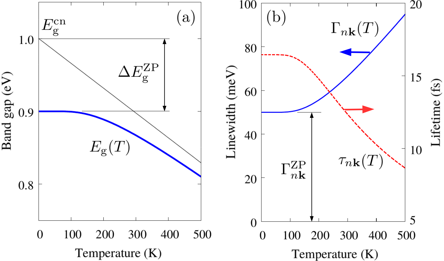
V.2.4 Carrier lifetimes
While the real part of the poles in Eq. (164) describes the energy level renormalization induced by the electron-phonon coupling, the imaginary part in Eq. (165) carries information on the spectral broadening, which will be discussed in Sec. (V.2.5), and on quasiparticle lifetimes, which we discuss below.
After transforming from Eq. (163) into the time domain it is seen that, for an electron or hole added to the system at time in the state , the probability amplitude to persist in the same state decreases as . Using Eqs. (157) and (165) it can be seen that for an electron added to the system and for a hole. Therefore the average time spent by the particle in the state is .
A popular expression for the electron and hole lifetimes is obtained by making the replacement in Eq. (157), and by taking the absolute value of the imaginary part. We find:
| (169) |
A more accurate expression is discussed after Eq. (174) in the next section. The extension of the above result to finite temperature is obtained by taking the absolute value of the imaginary part of Eq. (158):
| (170) |
We emphasize the change of sign in the third line, resulting from the analytic continuation to the retarded self-energy. Equation (170) coincides with the expression that one would obtain by using the standard Fermi golden rule Grimvall (1981). The intuitive interpretation of this result is that the quasiparticle lifetime is reduced by processes of phonon emission and absorption, corresponding to the second and third lines of Eq. (170), respectively. We note that in deriving Eq. (170) we did not consider the Debye-Waller self-energy; this is because the diagonal matrix elements of are purely real, hence they do not contribute to the quasiparticle widths Lautenschlager et al. (1986). Ab initio calculations of carrier lifetimes using Eq. (170) were first reported by Eiguren et al. (2002, 2003a). These applications and more recent developments will be reviewed in Sec. X.1.
If we evaluate Eq. (170) for the same simplified model introduced for the temperature renormalization, and we neglect the phonon energy in the Dirac delta functions, we obtain where is the linewidth at . The dependence of the linewidth and the corresponding lifetime on temperature for this model are shown in Fig. 3(b). This trend is typical in semiconductors Lautenschlager et al. (1987b, a).
V.2.5 Kinks and satellites
In many cases of interest, the use of Brillouin-Wigner perturbation theory as given by Eqs. (164)-(165) is not sufficient to provide an adequate description of EPIs, and it becomes necessary to go back to the complete Dyson equation, Eq. (163). Generally speaking a direct solution of the Dyson equation is important in all those cases where the electronic energy scales are comparable to phonon energies, namely in metals (including superconductors), narrow-gap semiconductors, and doped semiconductors. In order to study these systems, it is convenient to introduce an auxiliary function called the ‘spectral density function’, or simply spectral function.
In its simplest version the spectral function is defined as Abrikosov et al. (1975); Mahan (1993):
| (171) |
where the superscript ‘ret’ stands for ‘retarded’, and simply indicates that all poles of the Green’s function in the upper complex plane must be replaced by their complex conjugate. The spectral function is positive definite and carries the meaning of a ‘many-body momentum-resolved density of states’ Abrikosov et al. (1975). This is precisely the function that is probed by angle-resolved photoelectron spectroscopy experiments or ARPES Damascelli et al. (2003). Using Eq. (163) the spectral function can be rewritten as:
| (172) |
In order to obtain the correct spectral function, it is important to use the retarded self-energy. This is done by using Eq. (158) for the Fan-Migdal term, while the static Debye-Waller term remains unchanged.
It is often convenient to approximate the spectral function as a sum of quasiparticle peaks. To this aim, one performs a linear expansion of Eq. (172) around each quasiparticle energy , to obtain:
| (173) |
This is a sum of Lorentzians with strength and width . Here the ‘quasiparticle strength’ is defined as the homonymous quantity appearing in calculations Hedin and Lundqvist (1969):
| (174) |
The result expressed by Eq. (173) shows that, in a rigorous field-theoretic approach, the quasiparticle broadening and lifetime given by Eqs. (169) and (170) should be renormalized by and , respectively, and should be evaluated using the quasiparticle energy instead of . This result can also be derived from Eq. (165) by performing a Taylor expansion of the self-energy along the imaginary axis and using the Cauchy-Riemann conditions.
In order to illustrate the typical features of the spectral function, we consider a model system characterized by one parabolic conduction band. The occupied electronic states couple to all states within an energy cutoff via a dispersionless phonon mode and a constant electron-phonon matrix element. A simplified version of this model was discussed by Engelsberg and Schrieffer (1963) by considering a constant density of electronic states. By evaluating the spectral function in Eq. (172) using the Fan-Migdal self-energy and neglecting the Debye-Waller term, we obtain the results shown in Fig. 4 for two sets of parameters.
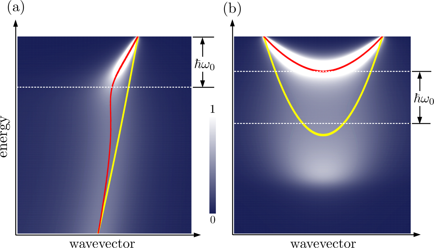
In Fig. 4(a) the Fermi energy is much larger than the characteristic phonon energy. This case is representative of a metallic system with electron bands nearly linear around the Fermi level. Here the electron-phonon interaction leads to (i) a reduction of the band velocity in proximity of the Fermi level, and (ii) a broadening of the spectral function beyond the phonon energy . A detailed analysis of these features for a slightly simpler model system, including a discussion of the analytic properties of the Green’s function, can be found in the work by Engelsberg and Schrieffer.
The solid line (red/dark gray) in Fig. 4(a) shows the renormalized band structure obtained from Brillouin-Wigner perturbation theory, Eq. (164). We see that these solutions track the maxima of the spectral function . The renormalized bands exhibit a characteristic ‘S-shape’ near the Fermi level, corresponding to multiple solutions of Eq. (164) for the same wavevector . Starting from the late 1990s such S-shaped energy-momentum dispersion curves have been observed in a number of ARPES experiments, and have become known in the literature as the ‘photoemission kink’ Valla et al. (1999a). First-principles calculations of kinks were first reported by Eiguren et al. (2003a); Giustino et al. (2008), and will be reviewed in Sec. VIII.
In Fig. 4(b) the Fermi energy is comparable to the characteristic phonon energy. This case is representative of a degenerately doped semiconductor close to a conduction band minimum. Here the electron-phonon interaction leads to two distinct spectral features: (i) a parabolic band with a heavier mass, which is well described by the Brillouin-Wigner solutions (solid line, red/dark gray), and (ii) a polaron satellite that is visible further down. In this example, it is clear that Eq. (164) is unable to describe the satellite, and that the spectral function carries qualitatively new information about the system. Polaron satellites resembling Fig. 4(b) have been observed in ARPES experiments on doped oxides (Moser et al., 2013; Chen et al., 2015; Cancellieri et al., 2016; Wang et al., 2016) and recently calculated from first principles Verdi et al. (2016).
V.2.6 Model Hamiltonians, polarons, and the cumulant expansion
At the end of this section it is worth mentioning complementary non first-principles approaches for studying the effects of EPIs on the electronic properties of solids. Model EPI Hamiltonians can be derived from Eq. (II) by choosing a priori explicit expressions for the electron band energies, the vibrational frequencies, and the coupling matrix elements. Examples of model Hamiltonians are those of Fröhlich (1954), Holstein (1959), Su, Schrieffer, and Heeger (1979), the Hubbard-Holstein model Berger et al. (1995), the Peierls-Hubbard model Campbell et al. (1984), the ‘-’ Holstein model Rösch and Gunnarsson (2004), and the Su-Schrieffer-Heeger-Holstein model Perroni et al. (2004). These models involve the tight-binding approximation, the Einstein phonon spectrum, and electron-phonon couplings to first order in the atomic displacements. Using these model Hamiltonians it is possible to go beyond the approximations introduced in Sec. V.2.2, and obtain non-perturbative solutions by means of canonical Lang-Firsov transformations, path-integral methods, exact diagonalization, variational or quantum Monte Carlo techniques Alexandrov (2008); Alexandrov and Devreese (2010). These models have been used extensively to explore many aspects of polaron physics, for example the ground-state energy of polarons (weak or strong coupling), their spatial extent (large or small polarons), and transport properties (band-like or hopping-like).
Given the considerable body of literature on model EPI Hamiltonians, it is natural to ask whether one could bring ab initio calculations of EPIs to a similar level of sophistication. The main limitation of current first-principles approaches is that, given the complexity of the calculations, the electron self-energies are evaluated using the bare propagators, as in Eq. (157). As a consequence, higher-order interaction diagrams beyond the Migdal approximation Migdal (1958) are omitted altogether.
A promising avenue for going beyond the Migdal approximation consists of introducing higher-order diagrams via the ‘cumulant expansion’ approach (Hedin and Lundqvist, 1969; Langreth, 1970; Aryasetiawan et al., 1996). In the cumulant expansion method, instead of calculating the electron Green’s function via a Dyson equation, one evaluates the time evolution of the Green’s function by formulating the problem in the interaction picture, in symbols: Aryasetiawan et al. (1996). The distinctive advantage of this approach is that the ‘cumulant’ can be obtained from a low-order self-energy, for example the Fan-Migdal self-energy in Eq. (157), and the exponential ‘resummation’ automatically generates higher-order diagrams (Mahan, 1993, pag. 523). Detailed discussions of the cumulant expansion formalism are given by Zhou et al. (2015) and Gumhalter et al. (2016).
The cumulant method provides an interesting point of contact between ab initio and model Hamiltonian approaches. In fact, the cumulant expansion is closely related to the ‘momentum average approximation’ introduced by Berciu (2006) for studying the Green’s function of the Holstein polaron.
The cumulant expansion has proven successful in ab initio calculations of electron-electron interactions, in particular valence band satellites in semiconductors (Kheifets et al., 2003; Guzzo et al., 2011, 2012, 2014; Lischner et al., 2013; Kas et al., 2014; Caruso et al., 2015, 2015b). In the context of EPIs, the ab initio cumulant expansion method has been applied to elemental metals by Story et al. (2014), and to the ARPES spectra of -doped TiO2 by Verdi et al. (2016). In the latter work the cumulant method correctly reproduced the polaron satellites observed in the experiments of Moser et al. (2013).
The study of polarons using ab initio many-body techniques is yet to begin, however a first calculation of the spectral function of Fröhlich polarons and an approximate polaron wavefunction have recently been reported by Verdi et al. (2016).
VI Efficient calculations of matrix elements and their integrals
The study of EPIs from first principles requires evaluating Brillouin-zone integrals of functions that exhibit strong fluctuations. This requirement can be appreciated by inspecting Eqs. (145) and (157): there the denominators become large whenever the difference between two electronic eigenvalues approaches a phonon energy. As a result, while in DFT total energy calculations the Brillouin zone is typically discretized using meshes of the order of 101010 points, the numerical convergence of EPI calculations requires much finer grids, sometimes with as many as wavevectors Giustino et al. (2007a); Poncé et al. (2015). Determining vibrational frequencies and perturbations for such a large number of wavevectors is a prohibitive task, since every calculation is roughly as expensive as one total energy minimization.
These difficulties stimulated the development of specialized numerical techniques for making calculations of EPIs affordable. In the following sections two such techniques are reviewed: electron-phonon Wannier interpolation and Fermi-surface harmonics.
VI.1 Wannier interpolation
VI.1.1 Maximally-localized Wannier functions
In addition to the standard description of electrons in solids in terms of Bloch waves, as in Eq. (29), it is possible to adopt an alternative point of view whereby electrons are described as linear combinations of localized orbitals called ‘Wannier functions’ Wannier (1937). The most general relation between Wannier functions and Bloch waves can be written as follows. One considers electron bands with eigenfunctions , where the index is restricted to a set of bands that are separated from all other bands by finite energy gaps above and below. These bands are referred to as ‘composite energy bands’ Marzari and Vanderbilt (1997). Wannier functions are defined as:
| (175) |
where is a unitary matrix in the indices and . From this definition and Eq. (213) it follows that Wannier functions are normalized in the supercell, . Furthermore, since is lattice-periodic, Wannier functions have the property . The inverse transformation of Eq. (175) is obtained by using the unitary character of together with Eq. (213):
| (176) |
The unitary matrix is completely arbitrary, therefore there exists considerable freedom in the construction of Wannier functions. For example by requiring that one can make Wannier functions real-valued. Marzari and Vanderbilt exploited this degree of freedom to construct Wannier functions that are maximally localized.
A comprehensive and up-to-date review of the theory and applications of maximally-localized Wannier functions (MLWFs) is given by Marzari et al. (2012). Here we only recall that, in order to minimize the spatial extent of a function in a periodic solid, one needs to use a modified definition of the position operator, since the standard position operator is unbounded in an infinite crystal. This procedure is now well-established and it is linked to the development of the modern theory of dielectric polarization King-Smith and Vanderbilt (1993); Resta (1994). Nowadays it is possible to determine MLWFs routinely Mostofi et al. (2008). The original algorithm of Marzari and Vanderbilt (1997) was also extended to deal with situations where a composite set of bands cannot be identified. This happens notably in metals for electronic states near the Fermi energy. For these cases, Souza et al. (2001) developed a band ‘disentanglement’ procedure, which extracts a subset of composite bands out of a larger set of states.
For the purposes of the present article, the most important property of MLWFs is that they are exponentially localized in insulators, in the sense that for large , with real parameters. This property was demonstrated in one spatial dimension by Kohn (1959a) and He and Vanderbilt (2001), and in two and three dimensions by Brouder et al. (2007), under the condition that the system exhibits time-reversal symmetry. In the case of metallic systems, no exponential localization is expected. However, the Wannier functions obtained in metals using the disentanglement procedure of Souza et al. (2001) are typically highly localized.
MLWFs are usually comparable in size to atomic orbitals, and this makes them ideally suited for Slater-Koster interpolation of band structures, as shown by Souza et al. (2001). This concept was successfully employed in a number of applications requiring accurate calculations of band velocities, effective masses, density of states, Brillouin-zone integrals, and transport coefficients (Wang et al., 2006; Yates et al., 2007; Wang et al., 2007; Pizzi et al., 2014).
VI.1.2 Interpolation of electron-phonon matrix elements
Wannier functions were introduced in the study of EPIs by Giustino et al. (2007b, a). The starting point is the definition of the electron-phonon matrix element in the Wannier representation:555 We note that has dimensions of energy by length, at variance with Eq. (38). For consistency here we use a definition that differs from that given in Giustino et al. (2007a) by a factor ; this factor is inconsequential.
| (177) |
where the subscript ‘sc’ indicates that the integral is over the BvK supercell. The relation between these quantities and the standard EPI matrix elements is found by replacing Eq. (176) inside Eq. (38), and using Eqs. (34)-(35) Giustino et al. (2007a):
| (178) |
where we defined and are the vibrational eigenmodes of Eq. (15). The inverse relation is:
| (179) |
with . The last two equations define a generalized Fourier transform of the electron-phonon matrix elements between reciprocal space and real space. In Eq. (179) we have and to indicate that the BvK supercells for electronic band structures and phonon dispersions may not coincide.
If the quantity decays rapidly as a function of and , then only a small number of matrix elements in the Wannier representation will be sufficient to generate anywhere in the Brillouin zone by means of Eq. (178). The dependence of the matrix elements on and can be analyzed by considering the following bound: . The first term guarantees that the matrix element decays in the variable at least as fast as MLWFs. As a result the worst case scenario corresponds to the choice . In this case, the matrix element decays with the variable at the same rate as the screened electric dipole potential generated by the atomic displacement . In non-polar semiconductors and insulators, owing to the analytical properties of the dielectric matrix Pick et al. (1970), this potential decays at least as fast as a quadrupole, that is . As a result, all matrix elements in reciprocal space are finite for Vogl (1976) and hence amenable to interpolation. In the case of metals the asymptotic trend of is dictated by Fermi-surface nesting, leading to Friedel oscillations that decay as (Fetter and Walecka, 2003, pp. 175–180). These oscillations are connected to the Kohn anomalies in the phonon dispersion relations Kohn (1959b). In practical calculations, Friedel oscillations are usually not an issue since they are suppressed by the numerical smearing of the Fermi-Dirac occupations, and a Yukawa-type exponential decay is recovered. The case of polar materials is more subtle and will be discussed in Sec. VI.1.3. Figure 5 illustrates the spatial decay of as a function of and for the prototypical case of diamond.
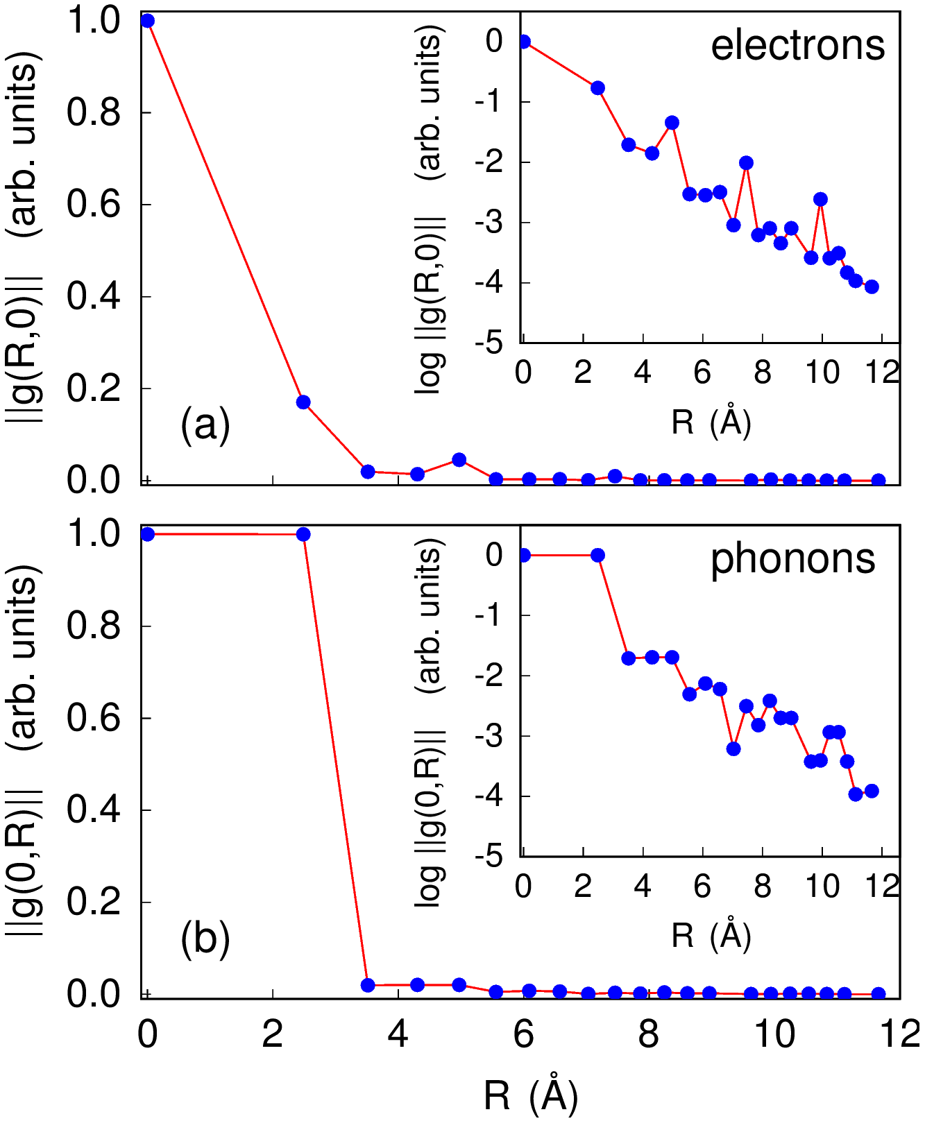
The interpolation strategy is entirely analogous to standard techniques for generating phonon dispersion relations using the interatomic force constants Gonze and Lee (1997): one first determines matrix elements in the Bloch representation using DFPT on a corse grid in the Brillouin zone, as in Sec. III.2.3. Then MLWFs are determined using the procedures of Marzari and Vanderbilt (1997); Souza et al. (2001). This yields the rotation matrices to be used in Eq. (179). The Fourier transform to real space is performed via Eq. (179). At this point, one assumes that matrix elements outside of the Wigner-Seitz supercell defined by the coarse Brillouin-zone grid can be neglected, and uses Eq. (178) in order to obtain the matrix elements on very fine grids. The last step requires the knowledge of the rotation matrices also on the fine grids; these matrices are obtained from the Wannier interpolation of the band structures, as described by Souza et al. (2001). The operation is computationally inexpensive and enables the calculation of millions of electron-phonon matrix elements. The procedure can now be applied routinely Noffsinger et al. (2010); Poncé et al. (2016). Figure 6 shows the matrix elements obtained using this method, as compared to explicit DFPT calculations.
Wannier interpolation of electron-phonon matrix elements was successfully employed in a number of applications, ranging from metal and superconductors to semiconductors and nanoscale systems.666 See for example (Park et al., 2007; Giustino et al., 2008; Park et al., 2008b; Noffsinger et al., 2009, 2010; Calandra et al., 2010; Giustino et al., 2010; Vukmirović et al., 2012; Noffsinger et al., 2012; Margine and Giustino, 2013, 2014; Park et al., 2014; Bernardi et al., 2014; Verdi and Giustino, 2015; Sjakste et al., 2015; Bernardi et al., 2015).
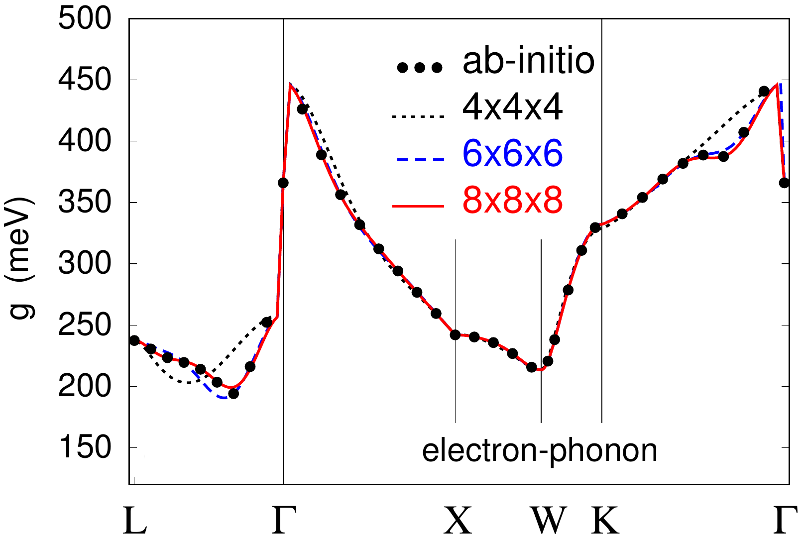
VI.1.3 Electron-phonon matrix elements in polar materials
In the case of polar materials, that is systems exhibiting nonzero Born effective charges Pick et al. (1970), the interpolation scheme discussed in Sec. VI.1.2 breaks down. In fact, in these systems the dominant contribution to the potential in Eq. (177) is a dipole, which decays as . As a consequence some of the matrix elements in reciprocal space diverge as for , and cannot be interpolated straightforwardly from a coarse grid to a fine grid. Physically this singularity corresponds to the ‘Fröhlich electron-phonon coupling’ Fröhlich (1954).
The adaptation of the Wannier interpolation method to the case of polar materials was recently given by Sjakste et al. (2015) and by Verdi and Giustino (2015). In both works the basic idea is to separate the matrix elements into a short-range contribution, , which is amenable to standard Wannier interpolation, and a long-range contribution, , which is singular and is dealt with analytically. The strategy is analogous to that in use for calculating LO-TO splittings in polar materials Gonze and Lee (1997). The starting point is to define the long-range component of the matrix elements by considering the potential generated by the Born charges of all the atoms, when displaced according to a given vibrational eigenmode. The derivation relies on standard electrostatics and can be found in Verdi and Giustino (2015):
In this expression and denote the Born effective charge tensors and the electronic permittivity tensor (that is, the permittivity evaluated at clamped nuclei). This expression is the generalization of Fröhlich’s model to the case of anisotropic crystalline lattices and multiple phonon modes Fröhlich (1954). The result can be derived alternatively using the analytical properties of the dielectric matrix Pick et al. (1970) as discussed by Vogl (1976).
In order to perform Wannier interpolation, one subtracts Eq. (VI.1.3) from the matrix elements computed on a coarse grid, interpolates the remainig short-range part, and then adds back Eq. (VI.1.3) on the fine grid. This process requires the interpolation of the brakets in the second line of Eq. (VI.1.3). Verdi and Giustino showed that, for small , these brakets can be interpolated via the relation , where the rotation matrices are obtained as usual from the procedure of Marzari and Vanderbilt (1997); Souza et al. (2001).777 Eq. (4) of Verdi and Giustino (2015) misses a factor ; this factor needs to be retained in order to correctly describe the acoustic modes near . In practical calculations the -vector sum in Eq. (VI.1.3) is restricted to small via the cutoff function ; the results are independent of the choice of the cutoff parameter . Figure 7 shows an example of Wannier interpolation for the prototypical polar semiconductor TiO2: it is seen that the singularity is correctly captured by the modified interpolation method.
At the end of this section, we mention that other interpolation schemes are equally possible (Eiguren and Ambrosch-Draxl, 2008b; Prendergast and Louie, 2009; Agapito et al., 2013; Gunst et al., 2016). For example Eiguren and Ambrosch-Draxl (2008b) proposed to interpolate only the local component of , while calculating explicitly the nonlocal part of the perturbation as well as the Kohn-Sham wavefunctions in the Bloch representation. Furthermore, Eq. (178) remains unchanged if MLWFs are replaced by a basis of localized atomic orbitals, and all the concepts discussed in this section remain valid. An interpolation scheme using local orbitals was recently demonstrated by Gunst et al. (2016).
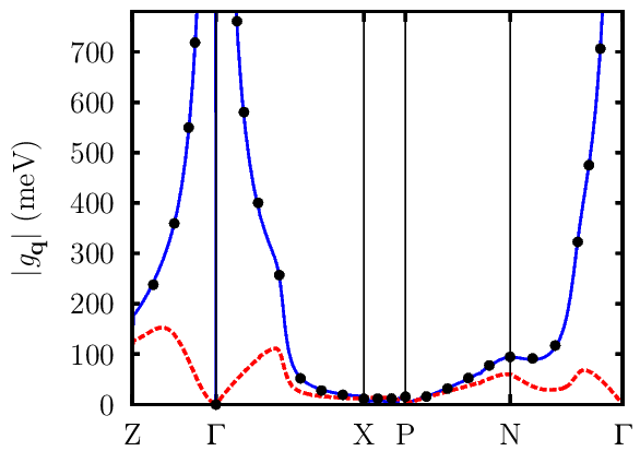
VI.2 Fermi surface harmonics
In the study of metallic systems, one is often interested in describing EPIs only for electronic states in the vicinity of the Fermi surface. In these cases, besides the Wannier interpolation discussed in Secs. VI.1.2-VI.1.3, it is possible to perform efficient calculations using ‘Fermi-surface harmonics’ (FSH). FSHs were introduced by Allen (1976) and recently revisited by Eiguren and Gurtubay (2014).
The basic idea underlying FSHs is to replace expensive three-dimensional Brillouin-zone integrals by inexpensive one-dimensional integrals in the energy variable. To this aim, Allen (1976) proposed to expand functions of the band index and wavevector , say , in products of pairs of functions, one depending on the energy, , and one depending on the wavevector, :
| (181) |
In this expression, the Fermi-surface harmonics (to be defined below) are constructed so as to obey the following orthogonality condition:
| (182) |
where is the density of states. Using Eqs. (181)-(182) one finds:
| (183) |
Allen showed that in the FSH representation a linear system of the kind transforms into . Linear systems of this kind are common in the solution of the Boltzmann transport equation (Sec. X) and the Eliashberg equations for the superconducting gap (Sec. XI.2). If one could perform the expansion using only a few harmonics, then the transformation would be advantageous, since the integrals over the wavevectors would have been absorbed in the expansion coefficients.
In the original proposal of Allen, the harmonics were defined as polynomials in the band velocities, however the completeness of the basis set was not established. In a recent work, Eiguren and Gurtubay (2014) proposed to construct these functions as eigenstates of a modified Helmholtz equation:
| (184) |
where is the band velocity for states at the Fermi surface, and is the eigenvalue for the harmonic . The new definition in Eq. (184) maintains the properties of the original FSHs, and carries the added advantage that the basis set is complete. In this case the subscript in labels the eigenstates of the Helmholtz equation. Eiguren and Gurtubay demonstrated the construction of ‘Helmholtz FSHs’ for prototypical metals such as Cu, Li, and MgB2.
VII Non-adiabatic vibrational frequencies and linewidths
As discussed in Secs. V.1.2-V.1.3, the electron-phonon interaction can lead to a renormalization of the adiabatic vibrational frequencies and to a broadening of the spectral lines.
The first ab initio investigations of the effects of the non-adiabatic renormalization of phonon frequencies were reported by Lazzeri and Mauri (2006) and Pisana et al. (2007). In these works the authors concentrated on the phonon of graphene, which is found at the wavenumber cm-1 at room temperature ( is the speed of light). This phonon corresponds to an in-plane C–C stretching vibration with , and has been studied extensively via Raman spectroscopy. In the graphene literature this mode is referred to as the ‘Raman band’. Figure 8 shows a comparison between calculated and measured phonon frequencies, as a function of doping, from Pisana et al. (2007). The calculations were performed (i) within the adiabatic approximation and (ii) by including the non-adiabatic frequency renormalization using Eq. (145).888 In the works reviewed in this section the authors used Eq. (145) with the bare matrix elements replaced by the screened matrix elements . All calculations were performed within DFT, using either the LDA or gradient-corrected DFT functionals. From Fig. 8 we see that the adiabatic theory is unable to reproduce the experimental data. On the contrary, the calculations including non-adiabatic effects nicely follow the measured Raman shift. This is a clear example of the limits of the adiabatic Born-Oppenheimer approximation and a demonstration of the importance of the phonon self-energy in Eq. (145).

The fact that the adiabatic approximation is inadequate for the phonon of doped graphene should have been expected from the discussion on p. V.1.3. In fact, graphene is a zero-gap semiconductor, therefore electrons residing in the vicinity of the Dirac points can make ‘virtual’ transitions with and energies comparable to that of the mode. As a result, the condition underlying the adiabatic approximation, , does not hold in this case.
The importance of non-adiabatic effects was confirmed also in the case of metallic single-walled carbon nanotubes (Piscanec et al., 2007; Caudal et al., 2007). In these works, the authors studied the phonon dispersion relations in the vicinity of , and they found that the difference between adiabatic and non-adiabatic dispersions is concentrated around the zone center. This finding is consistent with earlier models of non-adiabatic effects. In fact Maksimov and Shulga (1996) showed that, for metals with linear electron bands crossing the Fermi level, is only significant for wavevectors , where is the phonon energy and the Fermi velocity. This result can be derived from Eq. (145).
In the previous examples, the non-adiabatic renormalization of the vibrational frequencies is measurable but very small, typically of the order of 1% of the corresponding adiabatic frequencies. Saitta et al. (2008) considered the question as to whether one could find materials exhibiting large non-adiabatic renormalizations, and considered several graphite intercalation compounds, namely LiC6, LiC12, KC8, KC24, RbC8, CaC6, SrC6, BaC6, as well as other metallic systems such as MgB2, Mg, and Ti. In order to calculate the non-adiabatic renormalization at a reduced computational cost, the real part of the phonon self-energy was approximated as follows: , where stands for the average taken over the wavevectors in the Brillouin zone, and is the density of states at the Fermi level. This expression can be derived from Eq. (145) by replacing the bare matrix elements by their screened counterparts, and by neglecting the ‘interband’ contributions in the sum. Figure 9 shows a comparison between vibrational frequencies from experiment and those calculated with or without including the non-adiabatic self-energy. It is clear that the non-adiabatic frequencies are in much better agreement with experiment than the corresponding adiabatic calculations. Furthermore, in these compounds the renormalization can reach values as large as 300 cm-1. In contrast to this, the renormalization in Mg and Ti was found to be of only a few wavenumbers in cm-1.
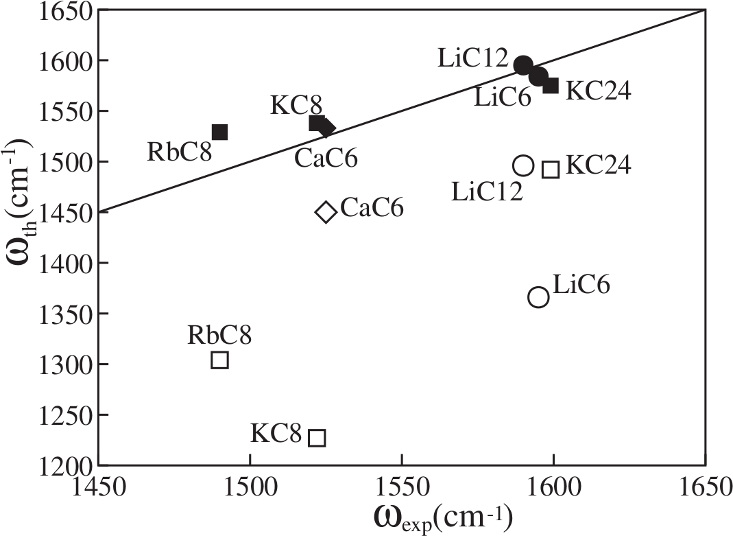
The case of MgB2 proved more puzzling: here the calculated non-adiabatic frequency is 761 cm-1, while experiments reported 600 cm-1. In order to explain this discrepancy, Saitta et al. reasoned that a more accurate calculation would require taking into account the relaxation time of the electrons, as pointed out by Maksimov and Shulga (1996). This would act so as to partly wash out non-adiabatic effects. In the field-theoretic language of Sec. V, this observation corresponds to stating that when one approximates the dressed electron propagator in Fig. 2(c) using the non-interacting Kohn-Sham Green’s function, one should include at the very least the effects of finite electron lifetimes (due to electron-electron, electron-impurity, and electron-phonon scattering), for example via the imaginary part of Eq. (157).
The calculations discussed so far in this section addressed the non-adiabatic renormalization of zone-center phonons. The generalization to calculations of complete phonon dispersions was made by Calandra et al. (2010). In their work, Calandra et al. employed Wannier interpolation (see Sec. VI) in order to calculate the non-adiabatic phonon self-energy of Eq. (145) throughout the Brillouin zone. Figure 10 shows a comparison between the standard DFPT phonon dispersion relations of CaC6 and the dispersions obtained after incorporating the non-adiabatic self-energy. It is seen that also in this case non-adiabatic effects are most pronounced at small , and can be as large as 7% of the adiabatic frequency.
In their work Calandra et al. approximated the bare matrix element appearing in Eq. (145) by the screened matrix element . This replacement was justified by reasoning that the error is of second-order in the induced electron density, hence it should be negligible.

The broadening of vibrational spectra arising from the electron-phonon interaction is almost invariably calculated from first principles using Eq. (146). Since the integration of the Dirac delta is computationally costly, it is common to rewrite that equation by neglecting the phonon energy in the delta function and by taking the low-temperature limit, as proposed by Allen (1972b):
| (185) |
where is the Fermi energy. Oddly enough, this is a sort of adiabatic approximation to the non-adiabatic theory. The main advantage is that this expression is positive definite, hence easier to converge numerically as compared to the complete expression in Eq. (146). The disadvantages are that the temperature dependence is lost, and that one cannot resolve fine features on the scale of a phonon energy. There exists a vast literature on first-principles calculations of phonon linewidths using Eq. (185), mostly in connection with electron-phonon superconductors.999 See for example early frozen-phonon calculations (Dacorogna et al., 1985b; Chang and Cohen, 1986; Lam et al., 1986) and more recent DFPT calculations (Savrasov et al., 1994; Bauer et al., 1998; Shukla et al., 2003; Heid et al., 2010). Earlier calculations not based on DFT are reviewed by Grimvall (1981). Equation (185) is now implemented in several large software projects Giannozzi et al. (2009); Gonze et al. (2009), and it is used routinely.
Phonon linewidths range from very small values such as 1 meV in Nb Bauer et al. (1998) to large values such as 30 meV in MgB2 Shukla et al. (2003). The agreement between calculations and neutron scattering or Raman measurements is usually reasonable.
Calculations of phonon linewidths using the more accurate expression in Eq. (146) are computationally more demanding and have been reported less extensively in the literature.101010 See for example the works of Lazzeri et al. (2006); Giustino et al. (2007a); Bonini et al. (2007); Park et al. (2008a).
So far we considered the effect of EPIs on the frequencies and lifetimes of vibrational excitations in solids. Another important phenomenon which modifies frequencies and lifetimes is anharmonicity. Anharmonic effects result from third and higher-order terms in the Taylor expansion of the total potential energy in the atomic displacements (Sec. III.1). These effects can be interpreted as additional interactions that couple the oscillators of the harmonic lattice; for example, third-order anharmonic effects reduce phonon lifetimes via energy up- or down-conversion processes involving three phonons.
Anharmonic effects can be described using a many-body field-theoretic formalism Cowley (1963), in complete analogy with the theory of EPIs discussed in Sec. IV. The calculation of anharmonic effects from first principles goes through the evaluation of third- and fourth-order derivatives of the total potential energy in the adiabatic approximation. Third-order coefficients are routinely computed using DFPT (Debernardi et al., 1995; Deinzer et al., 2003; Lazzeri et al., 2003; Broido et al., 2007; Bonini et al., 2007). In thoses cases where the harmonic approximation fails completely, ‘self-consistent phonon’ techniques can be employed Hooton (1955); Koehler (1966); recent implementations and calculations can be found in Errea et al. (2011, 2014), Hellman et al. (2011, 2013); Monserrat et al. (2013).
VIII Electron-phonon interactions in photoelectron spectroscopy
In Sec. V.2.5 we have seen how the electron-phonon interaction in metals can lead to band structure ‘kinks’ near the Fermi energy. This is illustrated by the model calculation in Fig. 4(a). The experimental investigation of these features started in the late 1990s, following the development of high-resolution angle-resolved photoelectron spectroscopy (ARPES). Since in ARPES only the component of the photoelectron momentum parallel to the sample surface is conserved Damascelli et al. (2003), complete energy vs. wavevector dispersion relations can be measured directly only for 2D or quasi-2D materials. Accordingly, the first observations of kinks were reported for the surface states of elemental metals111111Valla et al. (1999a); Hengsberger et al. (1999) and for the CuO2 planes of copper oxide superconductors.121212Valla et al. (1999b), Lanzara et al. (2001), Johnson et al. (2001). Ab initio calculations of ARPES kinks can be performed by using the diagonal part of the Fan-Migdal self-energy (the Debye-Waller self-energy will be discussed at the end of this section). To this aim, it is common to rewrite Eqs. (157)-(158) at finite temperature using a spectral representation:
| (186) |
Here the function is the so-called the ‘Eliashberg function’ and is defined as:
| (187) | |||||
This quantity is positive, temperature-independent, and contains all the materials-specific parameters. Physically it is proportional to the scattering rate of an electron in the state into any electronic state at the energy , by emitting or absorbing any one phonon of energy . One complication related to the Eliashberg function is that in the literature many variants of Eq. (187) can be found, each stemming from specific approximations; some of these expressions are summarized by Grimvall (1981, pp. 107–109).
The first ab initio calculations of the phonon-induced electron self-energies and photoemission kinks were reported by Eiguren et al. (2003a) for the surface state of the Be(0001) surface. Since the evaluation of Eqs. (186) and (187) is computationally demanding, Eiguren et al. employed simplified expressions which involve three approximations: (i) the Eliashberg function is replaced by its isotropic average, ; (ii) phonon energies are neglected next to electron energies (as in the adiabatic approximation), and (iii) particle-hole symmetry is assumed. Using these approximations the imaginary part of the Fan-Migdal self-energy becomes:
| (188) |
where the average of the self-energy is defined as for the Eliashberg function. The real part of the self-energy can be found starting from the same approximations, and is given by Grimvall (1981).

Figure 11 shows the self-energy of the surface state at the Be(0001) surface calculated by Eiguren et al. (2003a) using Eq. (VIII). The imaginary part resembles a step-function, with an onset around the energy threshold for phonon emission by a hole (40–80 meV in this case). At a qualitative level, this trend can be rationalized by replacing the Eliashberg function in Eq. (VIII) by a Dirac delta at a characteristic phonon energy . In this case, the hole self-energy becomes proportional to . At this is precisely a step function with onset at . The real part of the self-energy vanishes for , with being the largest phonon frequency. This can be seen in Fig. 11(b), and is a consequence of the approximation of particle-hole symmetry. Eiguren et al. also determined the renormalization of the surface state band structure arising from electron-phonon interactions, using Eq. (164); this is shown in the inset of Fig. 11(a). Overall the calculations of Eiguren et al. (2003a) showed good agreement with photoelectron spectroscopy experiments, both in the shape and magnitude of the self-energy LaShell et al. (2000).
In addition to the above calculations, several studies of the electron-phonon self-energy at metal surfaces were reported, namely for the Cu(111) and Ag(111) surfaces Eiguren et al. (2002), the Al(100), Ag(111), Cu(111), and Au(111) surfaces Eiguren et al. (2003b), and the W(110) surface Eiguren and Ambrosch-Draxl (2008a). Building on these studies, Eiguren et al. (2009) performed a detailed analysis of the self-consistent solutions of the complex Dyson equation for the quasiparticle energies, Eq. (164)-(165), and illustrated the key concepts in the cases of the W(110) surface and for the phonon-mediated superconductor MgB2.
Equation (VIII) or closely-related approximations were also employed in the study of electron and hole lifetimes in bulk Be Sklyadneva et al. (2005), Pb Sklyadneva et al. (2006), and Mg Leonardo et al. (2007); the photoemission kink in YBa2Cu3O7 Heid et al. (2008); and the spectral function of Ca-intercalated graphite Sanna et al. (2012).
In the case of complex systems the validity of the approximations (i)–(iii) leading to Eq. (VIII) is not warranted, and a direct calculation of the Fan-Migdal self-energy using Eqs. (186) and (187) is necessary. Calculations of the complete self-energy were reported by Park et al. (2007) for graphene, by Giustino et al. (2008) for the high-temperature superconductor La1-xSrxCu2O4, and by Margine et al. (2016) for Ca-intercalated bilayer graphene. Figure 12 shows the calculated self-energy and spectral function of graphene calculated by Park et al. (2007, 2009). The structure of the self-energy is similar to that shown in Fig. 11, with one important exception: does not vanish a few phonon energies away from the Fermi level, but tends instead towards a linear asymptote. Calandra and Mauri (2007) performed a combined ab initio/analytical study of the effects of the electron-phonon interaction on the electron bands of graphene and obtained very similar results. A linear asymptote in the real-part of the self-energy is a general feature of systems which do not exhibit particle-hole symmetry. For another example see the work on copper oxides by Giustino et al. (2008).
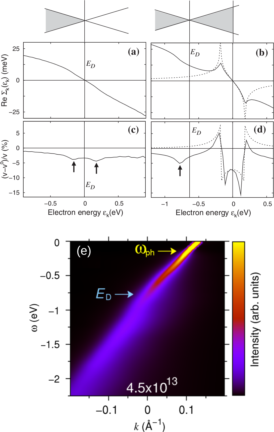
Using the Fan-Migdal self-energy, it is possible to calculate the renormalization of the band velocity induced by the electron-phonon interaction. Let us denote by the DFT band velocity and the band velocity after including electron-phonon interactions. Using Eq. (164) with we find that these two quantities are simply related by , where is the quasiparticle strength of Eq. (174), and is the ‘mass enhancement parameter’ or ‘electron-phonon coupling strength’ Grimvall (1981):
| (189) |
In the study of EPIs in metals, the coupling strength is of significant interest since it is related to the superconducting transition temperature of phonon-mediated superconductors (see Secs. VIII.1 and XI).
The velocity renormalization in graphene calculated using Eq. (189) is shown in Fig. 12(c) and (d), while a calculation of the complete spectral function is shown in Fig. 12(e). Here the characteristic photoemission kink is visible between 150–200 meV but it is not very pronounced, since in this case Park et al. (2009). These results are in good agreement with measured photoelectron spectra Bostwick et al. (2007); Zhou et al. (2007).
Incidentally, we remark that in the analysis of ARPES data it is common to extract the coupling strength directly from the ratio of the band velocities above and below the electron-phonon kink. However, this procedure is subject to a significant uncertainty, since the ‘bare’ velocity is not known and must be approximated by fitting the fully-interacting dispersions using ad hoc models. For example, in the vicinity of Van Hove singularities this procedure leads to a significant overestimation of the electron-phonon coupling strength (Park et al., 2008b; Bianchi et al., 2010).
In addition to photoemission kinks, recent ARPES measurements revealed the existence of polaron satellites in doped oxides, namely TiO2 Moser et al. (2013) and SrTiO3 Chen et al. (2015); Cancellieri et al. (2016); Wang et al. (2016). The phenomenology is similar to what was discussed in relation to Fig. 4(b). The first theoretical studies along this direction were reported by Story et al. (2014), who applied the cumulant expansion approach to the case of the electron-phonon self-energy; by Antonius et al. (2015) who identified satellites in the spectral functions of LiF and MgO; and by Verdi et al. (2016), who calculated the ARPES spectra of -doped TiO2.
At the end of this section, it is worth coming back to the Debye-Waller self-energy. So far we only discussed the Fan-Migdal self-energy, starting from Eq. (186), and we ignored the Debye-Waller self-energy appearing in Eq. (152). This omission reflects the fact that, in the literature on electron-phonon interactions in metals, the DW term has always been disregarded. In order to rationalize this approximation, we rewrite the DW self-energy as follows, by combining Eqs. (160) and (40):
| (190) |
with . The subscript ‘uc’ indicates that the integral is over one unit cell. From Eq. (190) we see that acts like a static local potential; indeed the first calculations including DW effects were performed by directly modifying the ionic pseudopotentials Antonc̆ík (1955); Walter et al. (1970). From Eq. (190) we also see that the only variation in the DW self-energy comes from the Bloch amplitudes . Let us consider the limiting situation of the homogeneous electron gas. In this case (Sec. III.2.5), therefore is a constant, independent of . This behavior should be contrasted with the Fan-Migdal self-energy, which exhibits significant structure near the Fermi energy, as it can be seen in Fig. 4.
In more realistic situations, such as doped semiconductors, perturbation theory Kittel (1963) can be used to show that varies smoothly as a function of within the same band. In contrast with this scenario, exhibits large variations across different bands. This carries important consequences for the calculation of temperature-dependent band gaps (Sec. IX.1.1).
VIII.0.1 Electron mass enhancement in metals
We now come back to the mass enhancement parameter introduced in Eq. (189), since this quantity played a central role in the development of the theory of EPIs in metals.
The notion of ‘mass enhancement’ becomes clear when we consider a parabolic band as in the model calculations of Fig. 4. Near the Fermi surface the non-interacting dispersions are given by , where is a wavevector on the Fermi surface, and the electron velocity is . After taking into account the EPI, the electron velocity is renormalized to . Since the magnitude of the Fermi momentum is unchanged (see caption of Fig. 4) this renormalization can be interpreted as an effective increase of the band mass from to . This reasoning holds for metals with parabolic bands and for doped semiconductors near band extrema, and does not take into account the Debye-Waller self-energy.
The electron mass enhancement is reflected into the increase of the heat capacity of metals at low temperature. In fact, below the Debye temperature the electronic contribution to the heat capacity dominates over the lattice contribution Kittel (1976). Since the heat capacity is proportional to the density of states at the Fermi level, and the density of states is inversely proportional to the band velocity, it follows that the heat capacity is directly proportional to the electron mass. This property can be used as a means to determine the strength of the electron-phonon coupling in simple metals from specific heat measurements Grimvall (1975).
The general theory of the effects of electron-phonon interactions on the heat capacity and other thermodynamic functions was developed by Eliashberg (1963), Prange and Kadanoff (1964), and Grimvall (1969). A field-theoretic analysis of the effect of EPIs on thermodynamic functions was developed by Eliashberg (1963) starting from the identities of Luttinger and Ward (1960) in the zero-temperature limit. Eliashberg’s analysis was subsequently extended to all temperatures by Grimvall (1969). Here we only quote Grimvall’s result relating the electronic entropy to the Fan-Migdal self-energy of Sec. V.2.1:
| (191) |
In order to derive this relation, Grimvall started by expressing the thermodynamic potential of the coupled electron-phonon system in terms of the electron and phonon propagators and self-energies, and identified the electronic contribution by neglecting terms of order as well as electron-electron interactions (Grimvall, 1969, Appendix).
Below the Debye temperature, an explicit expression for the entropy in Eq. (191) can be obtained by noting that the function is nonvanishing only for ; in this range Eq. (189) yields , therefore the integration in Eq. (191) can be carried out explicitly. As a result, the low-temperature heat capacity can be written as:
| (192) |
If we ignore the EPI by setting , this expression reduces to the standard textbook result for the free electron gas Kittel (1976). At high temperature Eq. (192) is no longer valid, and one has to evaluate the integral in Eq. (191) using the complete frequency-dependent FM self-energy. The main result of this procedure is that at high temperature the electronic heat capacity is no longer renormalized by EPIs. A detailed discussion of this aspect is provided by Grimvall (1969; 1981).
IX Electron-phonon effects in the optical properties of semiconductors
IX.1 Temperature dependence of band gaps and band structures
IX.1.1 Perturbative calculations based on the Allen-Heine theory
In Sec. V.2.3 we discussed how the electron-phonon interaction induces a ‘renormalization’ of the electronic energy levels, and thereby gives rise to ‘temperature-dependent band structures’. These effects have been studied in detail using the Fan-Midgal and the Debye-Waller self-energies, either via the Raleigh-Schrödinger approximation to Eq. (166), or via its adiabatic counterpart given by Eq. (167).
Equation (167) was first employed in a number of calculations based on empirical pseudopotentials, following the seminal work of Allen and Heine (1976). The key references can be found on p. 4, footnote. Allen and Cardona (1981) offer a clear introduction to the basic theory, a discussion of the computational methodology, as well as an historical perspective on earlier calculations.
The evaluation of the Debye-Waller contribution to the self-energy requires the calculation of the second-order variations of the Kohn-Sham potential with respect to the ionic displacements, Eq. (40). From a computational standpoint, this is challenging because one would have to use second-order DFPT, as discussed at the end of Sec. III.2.3. In order to avoid this complication, it is common practice to recast all second-order derivatives as products of first-order derivatives. This strategy was introduced by Allen and Heine in the case of monoatomic crystals, and extended to polyatomic unit cells by Allen and Cardona. The key observation behind this approach is that one can impose translational invariance of the theory to second order in the nuclear displacements. Specifically, the variation of the Kohn-Sham eigenvalues ensuing an arbitrary displacement of the nuclei should not change if all nuclei are further displaced by the same amount. Using time-independent perturbation theory, this condition yields the following two sum rules:
| (193) | |||
| (194) |
Here is a short-hand notation for and similarly for the second derivative; the primed summation indicates that eigenstates such that are skipped. The first sum rule is equivalent to stating that the electron-phonon matrix elements associated with the three translational modes at must vanish; this is an alternative formulation of the ‘acoustic sum rule’. The second sum rule, Eq. (194), suggests to express the matrix elements of the second derivatives of the potential in terms of first-order derivatives. However, Eq. (194) cannot be used as it stands, since it involves a sum of matrix elements on the left-hand side. In order to proceed, Allen and Heine employed the ‘rigid-ion’ approximation, whereby is written as a sum of atom-centered contributions (see Sec. II.1.1). Under this approximation all the terms on the left-hand side of Eq. (194) are neglected, and an explicit expression for is obtained.
In view of practical DFT implementations, Giustino et al. (2010) used the sum rule in Eq. (194) in order to rewrite the Debye-Waller self-energy as follows:
| (195) |
Here is an ‘effective’ matrix element, and it is obtained from the standard DFPT matrix elements by means of inexpensive matrix multiplications:
| (196) | |||||
| (197) | |||||
| (198) |
In the case of the three translational modes at , these definitions are replaced by , see the discussion at the end of p. B. The derivation of Eqs. (195)-(198) requires using Eqs. (20), (33)-(35), and (38), as well as taking the canonical average over the adiabatic nuclear quantum states.
Equation (195) involves a summation over unoccupied Kohn-Sham states, and so does the Fan-Migdal self-energy in Eq. (167). The numerical convergence of these sums is challenging, since one needs to evaluate a very large number of unoccupied electronic states. To address this issue, Gonze et al. (2011) developed a procedure whereby only a subset of unoccupied states is required, along the lines of the DFPT equations of Sec. III.2.3.
The first ab initio calculations using the formalism of Allen and Heine were reported by Marini (2008), who investigated the temperature dependence of the optical absorption spectrum of silicon and boron nitride. In this work Marini included excitonic effects by combining the Bethe-Salpeter formalism Onida et al. (2002) with the Allen-Heine theory, and obtained good agreement with experiments by calculating the direct absorption peaks using DFT/LDA phonons and matrix elements (indirect optical absorption will be discussed in Sec. IX.2).
The second application of the Allen-Heine theory using DFT/LDA was reported by Giustino et al. (2010) for the case of diamond. Here the authors investigated the temperature dependence of the direct band gap of diamond, and found that the Fan-Migdal and the Debye-Waller self-energies are of comparable magnitude. The calculations captured the characteristic Varshni effect (Fig. 3), and were able to reproduce the measured redshift of the band gap in the temperature range 80-800 K. These calculations were based on the adiabatic version of the Allen-Heine theory, and employed Eqs. (196)-(198) for the Debye-Waller self-energy. The calculations by Giustino et al. confirmed the large ( eV) zero-point renormalization of the direct gap of diamond predicted by Zollner et al. (1992) using the empirical pseudopotential method.
The unusually large zero-point correction to the electronic structure of diamond stimulated further work on this system: Cannuccia and Marini (2011, 2012) calculated the gap renormalization in diamond by employing both the adiabatic version of the Allen-Heine theory, as well as the non-adiabatic Green’s function approach, as described in Sec. V.2.5. Their calculations confirmed the large zero-point renormalization, and showed that the adiabatic theory underestimates the effect to some extent. Cannuccia and Marini (2012; 2013) also analyzed the quasiparticle renormalization and the spectral function.
Antonius et al. (2014) revisited the electron-phonon interaction in diamond by assessing the reliability of the rigid-ion approximation and the importance of many-body quasiparticle corrections to the DFT/LDA band structure. The main findings were that the rigid-ion approximation introduces a very small error in diamond, of the order of 10 meV, while quasiparticle corrections can increase the electron-phonon renormalization of the band gap by as much as 200 meV. The temperature dependence of the band gap of diamond calculated by Antonius et al. is shown in Fig. 13.
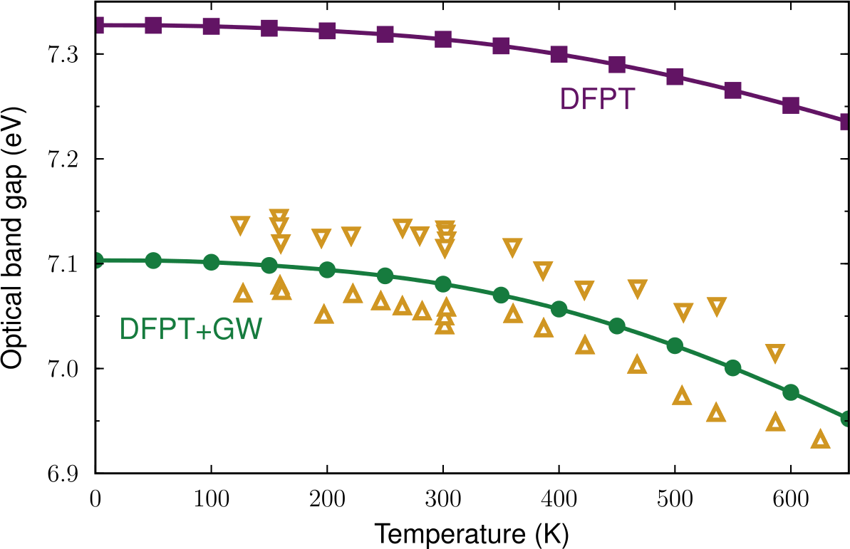
Further work on diamond was reported by Poncé et al. (2014b), who compared ab initio calculations based on the Allen-Heine theory with explicit frozen-phonon calculations (Sec. IX.1.2). The corrections to the rigid-ion approximation were found to be smaller than 4 meV in all cases considered. Poncé et al. (2014b, a) also reported a detailed assessment of the accuracy of the various levels of approximation in the calculation of the zero-point renormalization of energy levels, as well as a thorough comparison between the results of different first-principles implementations.
The electron-phonon renormalization of band structures was also investigated in a number of other systems. For example Kawai et al. (2014) studied zinc-blend GaN by combining the Allen-Heine theory with the Bethe-Salpeter approach. Poncé et al. (2015) investigated silicon, diamond, BN, -AlN, and -AlN using both the adiabatic version of the Allen-Heine theory and the non-adiabatic Green’s function method of Eqs. (157)-(158). Friedrich et al. (2015) investigated the zero-point renormalization in LiNbO3 using the adiabatic Allen-Heine theory. Villegas et al. (2016) studied the anomalous temperature dependence of the band gap of black phosphorous. Antonius et al. (2015) investigated diamond, BN, LiF, and MgO, focusing on the dynamical aspects and the spectral function (see Sec. VIII). The works by Poncé et al. (2015); Antonius et al. (2015) were the first to report complete band structures at finite temperature.
In Poncé et al. (2015) the authors paid special attention to the numerical convergence of the self-energy integrals with respect to the limit of the broadening parameter; they noted that in the case of polar crystals the adiabatic correction to the electron energies of band extrema, as given by Eq. (167), diverges in the limit of dense Brillouin-zone sampling. This behavior stems from the polar singularity in the electron-phonon matrix elements, Eq. (VI.1.3). In fact, near band extrema the bands are approximately parabolic, and the integrand in the adiabatic Fan-Migdal self-energy goes as for , while the volume element goes only as . This problem can be avoided by first performing the integration over in principal value, without neglecting phonon frequencies, and then taking the limit so as to recover the adiabatic approximation (Fan, 1951, Sec. IV); in this way the adiabatic approximation can still be employed without incurring into a singularity in the calculations. A practical strategy to correctly perform the principal value integration in first-principles calculations was recently proposed by Nery and Allen (2016); here the authors treat the singularity via an explicity analytic integration near . The complications arising in polar materials can also be avoided at once by using directly the more accurate expression in Eq. (166) based on Brillouin-Wigner perturbation theory, or even better by calculating the spectral functions as in Kawai et al. (2014); Antonius et al. (2015). In particular, Eq. (166) shows that in more accurate approaches the infinitesimal should be replaced by the finite physical linewidth .
Although temperature-dependent band structures of polar materials were recently reported Kawai et al. (2014); Poncé et al. (2015); Antonius et al. (2015), the specific role of the Fröhlich coupling discussed in Sec. VI.1.3 received only little attention so far. The only ab initio investigations which specifically addressed the role of polar couplings in this context are from Botti and Marques (2013) and Nery and Allen (2016). In order to understand the strategy of Botti and Marques, we refer to the Hedin-Baym equations in Sec. IV.2.1. Botti and Marques proposed that, instead of splitting the screened Coulomb interaction into electronic and nuclear contributions as in Eq. (104), one could try to directly calculate the screened Coulomb interaction including the lattice screening, as in Eqs. (85) and (86). In order to make the calculations tractable, Botti and Marques evaluated the total dielectric matrices using a simplified model based on the Lyddane-Sachs-Teller relations. The resulting formalism combines calculations and experimentally measured LO-TO splittings. The zero-point renormalization of the band gaps calculated by Botti and Marques for LiF, LiCl, NaCl, and MgO were all eV. This is an interesting result and deserves further investigation. We note incidentally that the Allen-Heine theory and that of Botti and Marques can both be derived from the Hedin-Baym equations. Therefore the approach of Botti and Marques should effectively correspond to calculating the Fan-Migdal self-energy by retaining only the long-range part of the polar electron-phonon matrix elements. In the case of the work by Nery and Allen (2016), the authors reported a Fröhlich contribution to the zero-point renormalization of the band gap of GaN of 45 meV, to be compared with the total renormalization arising from all modes of 150 meV.
IX.1.2 Non-perturbative adiabatic calculations
An alternative approach to the calculation of temperature-dependent band structures consists of avoiding perturbation theory and electron-phonon matrix elements altogether, and replacing the entire methodology discussed in Sec. IX.1.1 by straightforward finite-differences calculations. To see how this alternative strategy works we perform a Taylor expansion of the Kohn-Sham eigenvalues to second order in the atomic displacements , and then average the result on a nuclear wavefunction identified by the quantum numbers . After using Eq. (20) one obtains:
| (199) |
where we used the formal definition , and the variations are the same as in Eqs. (33)-(35). The nuclear wavefunctions are obtained from the ground-state in Eq. (223) by applying the ladder operators, as discussed in Appendix B. The above expression can be generalized to finite temperature by considering a canonical average over all possible nuclear states. The result maintains the same form as in Eq. (199), except that we now have the Bose-Einstein occupations (see footnote 3). Equation (199) is precisely the conceptual starting point of the Allen-Heine theory of temperature-dependent band structures, and appeared for the first time in Allen and Cardona (1981). If the variations are calculated in second-order perturbation theory, one obtains precisely the formalism of Allen and Heine.
It has been proposed that the coefficients could alternatively be obtained from the derivatives of the vibrational frequencies with respect to the electronic occupations, Allen and Hui (1980); King-Smith et al. (1989); Poncé et al. (2014b). A formal derivation of the link between these alternative approaches can be found in (Allen and Hui, 1980, Appendix; the authors refer to this as Brooks’ theorem). Incidentally, the first ab initio calculation of temperature-dependent band gaps relied on this approach King-Smith et al. (1989).
Most commonly, the coefficients in Eq. (199) are evaluated using frozen-phonon supercell calculations, via the second derivative of the eigenvalue with respect to collective atomic displacements along the vibrational eigenmodes . This approach was employed by Capaz et al. (2005) to study the temperature dependence of the band gaps in carbon nanotubes (within a tight-binding model), and by Han and Bester (2013) to obtain the zero-point renormalization and temperature dependence of the gaps of silicon and diamond quantum dots. Recent examples include works on diamond, silicon, SiC Monserrat and Needs (2014), as well as CsSnI3 Patrick et al. (2015).
Frozen-phonon supercell calculations based on Eq. (199) carry the advantage that the rigid-ion approximation, which is necessary to obtain Eqs. (195)-(198), is no longer required. Therefore this approach is more accurate in principle. In practice, however, the calculations are challenging as they require large supercells, and the derivatives must be evaluated for every vibrational mode of the supercell. Several computational strategies were developed to tackle this challenge. Patrick and Giustino (2013) proposed to perform the averages leading to Eq. (199) via importance-sampling Monte Carlo integration. Monserrat (2016b) described a constrained Monte Carlo scheme which improves the variance of the Monte Carlo estimator. Recently Zacharias and Giustino (2016) showed that it is possible to perform these calculations more efficiently by replacing the stochastic sampling by a suitable choice of an ‘optimum’ configuration; the result becomes exact in the thermodynamic limit of large supercells. In order to reduce the computational cost associated with the use of large supercells, Lloyd-Williams and Monserrat (2015) introduced ‘non-diagonal’ supercells, which allow one to access phonon wavevectors belonging to a uniform grid of points using supercells containing only unit cells.
The merit of these non-perturbative approaches is that they treat explicitly the nuclear wavefunctions, and enable exploring effects which go beyond the Allen-Heine theory. For example Monserrat et al. (2013, 2014, 2015) and Engel et al. (2015) were able to investigate effects beyond the harmonic approximations in several systems, such as LiH, LiD, high-pressure He, molecular crystals of CH4, NH3, H2O, HF, as well as Ice. In all these cases the authors found large zero-point effects on the band gaps.
Finally, we mention that the calculation of electronic properties at finite temperature via the Allen-Heine theory and its variants is closely related to what one would obtain using path-integral molecular dynamics simulations Della Sala et al. (2004); Ramírez et al. (2006, 2008), or even classical molecular dynamics simulations at high enough temperatures Franceschetti (2007).
IX.2 Phonon-assisted optical absorption
In addition to modifying the electron energy levels in solids, the electron-phonon interaction plays an important role in the optical properties of semiconductors and insulators, as it is responsible for phonon-assisted optical transitions. Phonon-assisted processes could be analyzed by considering the many-body electronic screening function in Eq. (95), by using the electron Green’s function dressed by the electron-phonon self-energy as in Eq. (151). Since this would require us a lengthy detour, here we simply reproduce the standard result of second-order time-dependent perturbation theory Bassani and Parravicini (1975); Ridley (1993):
| (200) |
In this expression is the absorption coefficient for visible light, e is the photon polarization, are the matrix elements of the electron velocity operator, and is the real part of the refractive index. The two denominators in the second line corresponds to indirect processes whereby a photon is absorbed and a phonon is absorbed or emitted (left), and processes whereby a phonon is absorbed or emitted, and subsequently a photon is absorbed (right). The above expression relies on the electric dipole approximation and is therefore valid for photon energies up to a few electronvolts. The theory leading to Eq. (200) was originally developed by Hall, Bardeen, and Blatt (1954).
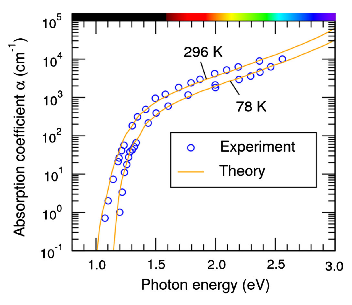
The first ab initio calculation employing Eq. (200) was reported by Noffsinger et al. (2012) for the prototypical case of silicon. The authors employed DFT for computing phonons and electron-phonon matrix elements, and the method for the quasiparticle band structures. The sampling of the Brillouin zone was achieved by means of the interpolation strategy described in Sec. VI. Figure 14 shows that the calculations by Noffsinger et al. are in very good agreement with experiment throughout the energy range of indirect absorption.
Further work along similar lines was reported by Kioupakis et al. (2010), who calculated the indirect optical absorption by free carriers in GaN; and Peelaers et al. (2015), who studied the indirect absorption by free carriers in the transparent conducting oxide SnO2. Recently, the ab initio theory of phonon-assisted absorption was also extended to the case of indirect Auger recombination by Kioupakis et al. (2015).
One limitation of the theory by Hall et al. is that the indirect absorption onset is independent of temperature. This is seen by noting that the Dirac delta functions in Eq. (200) contain the band structure energies at clamped nuclei. The generalization to incorporate temperature-dependent band structures as discussed in Sec. IX.1.1 is nontrivial. Patrick and Giustino (2014); Zacharias and Giustino (2016) showed that the electron-phonon renormalization of the band structure modifies the energies of real transitions but leaves unchanged the energies of virtual transitions; in other words the Allen-Heine renormalization should be incorporated only in the Dirac delta functions and in the first denominator in Eq. (200). In order to avoid these complications at once, Zacharias et al. (2015) developed an alternative approach which relies on the ‘semiclassical’ approximation of Williams (1951) and Lax (1952). In this approximation, the initial states in the optical transitions are described quantum-mechanically, and the final states are replaced by a quasiclassical continuum. In the formulation of Zacharias et al. the imaginary part of the temperature-dependent dielectric function takes the form:
| (201) |
where denotes the imaginary part of the dielectric function at clamped nuclei, and the expectation values have the same meaning as in Eq. (199). is the energy of the quantum nuclear state specified by the quantum number and is the canonical partition function. Zacharias et al. demonstrated that this approach provides an adiabatic approximation to Eq. (200), and seamlessly includes the temperature dependence of the electronic structure within the Allen-Heine theory. Using techniques similar to those of Sec. IX.1.2, the authors calculated the indirect optical absorption lineshape of silicon at various temperatures and obtained very good agreement with experiment. These results were recently extended to the temperature-dependent optical spectra of diamond and gallium arsenide by Zacharias and Giustino (2016).
X Carrier dynamics and transport
X.1 Electron linewidths and lifetimes
In Sec. V.2.4 we have seen how the Fan-Migdal self-energy can be used in order to evaluate the quasiparticle lifetimes (or equivalently linewidths) resulting from the electron-phonon interaction. The first ab initio calculations of this kind were reported by Eiguren et al. (2002, 2003a) in the study of the decay of metal surface states, and by Sklyadneva et al. (2005, 2006) and Leonardo et al. (2007) in the study of electron lifetimes of elemental metals. Some of these calculations and the underlying approximations were reviewed in Sec. VIII. Calculations of quasiparticle linewidths were also employed to study the temperature-dependent broadening of the optical spectra in semiconductors. For example Giustino et al. (2010) and Poncé et al. (2015) investigated the broadening of the direct absorption edge of diamond and silicon, respectively. In both cases good agreement with experiment was obtained. More recently, the same approach was employed to study the broadening of photoluminescence peaks in lead-iodide perovskites Wright et al. (2016). In this case, it was found that the standard Fermi golden rule expression, Eq. (170), significantly overestimates the experimental data. The agreement with experiment is restored by taking into account the quasiparticle renormalization ; see discussion following Eq. (174).
While these works were primarily concerned with the broadening of the spectral lines in photoemission or optical experiments, Eq. (170) can also be used to study carrier lifetimes in time-resolved experiments. The first ab initio study in this direction was reported from Sjakste et al. (2007), who investigated the thermalization of hot electrons in GaAs and the exciton lifetimes in GaP. In the case of GaAs, Sjakste et al. found thermalization rates in quantitative agreement with time-resolved luminescence and transient optical absorption measurements. Work along similar lines was also reported for the intervalley scattering times in Ge Tyuterev et al. (2011). Recently, the thermalization rates of hot electrons in GaAs were revisited by Bernardi et al. (2015). The authors employed Eq. (170) and the Wannier interpolation technique described in Sec. VI in order to finely sample the electron-phonon scattering processes near the bottom of the conduction band, see Fig. 15. Based on these calculations they were able to interpret transient absorption measurements in terms of the carrier lifetimes within each valley. Another interesting application of Eq. (170) was reported by Bernardi et al. (2014), who investigated the rate of hot carrier thermalization in silicon, within the context of photovoltaics applications.
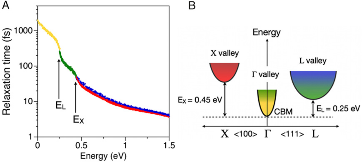
Very recently Sangalli and Marini (2015a, b) employed the lifetimes calculated using Eq. (170) in order to study carrier dynamics in silicon in real time. Strictly speaking, these developments lie outside of the scope of equilibrium Green’s functions discussed in Sec. IV, and require concepts based on non-equilibrium Green’s functions Kadanoff and Baym (1962). However, the basic ingredients of the electron-phonon calculations remain unchanged.
In all calculations discussed in this section, the electron-phonon matrix elements were obtained within DFT. However, in order to accurately describe electron-phonon scattering near band extrema Bernardi et al. (2014, 2015) and Wright et al. (2016) employed quasiparticle band structures. This is important in order to obtain accurate band effective masses, which affect the carrier lifetimes via the density of states.
X.2 Phonon-limited mobility
The carrier lifetimes of Eq. (170) are also useful in the calculation of electrical mobility, conductivity, and resistivity, within the context of the semiclassical model of electron dynamics in solids Ashcroft and Mermin (1976). In the semiclassical model, one describes the electronic response to an external perturbation by taking the fermionic occupations to represent the probability density function in the phase space defined by the unperturbed band structure. The probabilities are then determined using a standard Boltzmann equation. A comprehensive discussion of these methods can be found in the classic book of Ziman (1960).
Here we only touch upon the key result which is needed in ab initio calculations of electrical conductivity. In the semiclassical model, the electrical current is calculated as . In the absence of external fields and thermal gradients, the occupations reduce to the standard Fermi-Dirac occupations at equilibrium, , and the current vanishes identically. Upon introducing an electric field , the electrons respond by adjusting their occupations. In this model it is assumed that the variation is so small that the electronic density is essentially the same as in the unperturbed system. The modified occupations can be calculated using the linearized Boltzmann transport equation Ziman (1960):
| (202) |
where the kernel is defined as:
| (203) |
The left-hand side of Eq. (202) represents the collisionless term of the Boltzmann equation, that is the change in occupations due to the particle drift under the electric field. The right-hand side represents the change of occupations resulting from electrons scattered in or out of the state by phonon emission or absorption. The rates in Eq. (203) are simply derived from Fermi’s golden rule Grimvall (1981). By solving Eq. (202) self-consistently for all it is possible to calculate the current, and from there the conductivity. The connection with the carrier lifetimes of Eq. (170) is obtained within the so-called ‘energy relaxation time approximation’. In this approximation the incoming electrons are neglected in Eq. (202), that is the last term in the second line is ignored. As a result the entire right-hand side of the equation simplifies to .
The direct solution of Eq. (202) is computationally challenging, and fully ab initio calculations were reported only very recently by Li (2015) for Si, MoS2, and Al, and by Fiorentini and Bonini (2016) for -doped Si. Figure 16 shows that the mobility of -type silicon calculated by Li is in good agreement with experiment. The theory overestimates the measured values to some extent, and this might have to do with the limitations of the DFT matrix elements (see Sec. XII). In addition to the carrier mobility, Fiorentini and Bonini employed the ab initio Boltzmann formalism to calculate thermoelectric properties, such as the Lorenz number and the Seebeck coefficient.
The first ab initio calculation of mobility was reported by Restrepo et al. (2009) for the case of silicon, within the energy relaxation time approximation. Other recent calculations using various approximations to Eq. (202) focused on silicon (Wang et al., 2011; Liao et al., 2015), graphene (Borysenko et al., 2010; Park et al., 2014; Sohier et al., 2014; Restrepo et al., 2014; Gunst et al., 2016; Kim et al., 2016), MoS2 (Kaasbjerg et al., 2012; Li et al., 2013; Restrepo et al., 2014; Gunst et al., 2016), silicene (Li et al., 2013; Gunst et al., 2016), SrTiO3 and KTiO3 (Himmetoglu et al., 2014; Himmetoglu and Janotti, 2016).
Ab initio calculations of the resistivity of metals are less challenging than for semiconductors, and started appearing already with the work of Bauer et al. (1998). Most calculations on metals are based on Ziman’s resistivity formula, see Grimvall (1981, p. 210). An interesting recent example can be found in the work by Xu and Verstraete (2014) on the transport coefficients of lithium. We also highlight related work on phonon-limited transport in organic crystals (Hannewald and Bobbert, 2004a, 2004b; Ortmann et al., 2009; Vukmirović et al., 2012).

XI Phonon-mediated superconductors
The last application of ab initio calculations of EPIs that we will consider is the study of phonon-mediated superconductivity Schrieffer (1983). This research field is so vast that any attempt at covering it in a few pages would not make justice to the subject. For this reason, it was decided to limit the discussion to those novel theoretical and methodological developments which are aiming at fully predictive calculations, namely the ‘anisotropic Migdal-Eliashberg theory’ (Sec. XI.2), and the ‘density functional theory for superconductors’ (Sec. XI.3). For completeness, in Sec. XI.1 we also summarize the most popular equations employed in the study of phonon-mediated superconductors. All calculations described in this section were performed at the DFT level.
XI.1 McMillan/Allen-Dynes formula
Most ab initio calculations on phonon-mediated superconductors rely on a semi-empirical expression for the critical temperature, first introduced by McMillan (1968) and then refined by Allen and Dynes (1975):
| (204) |
Here is the superconducting critical temperature, is a ‘logarithmic’ average of the phonon frequencies Allen and Dynes (1975), is the electron-phonon ‘coupling strength’, and is a parameter describing the Coulomb repulsion. The functional form of Eq. (204) was derived by McMillan by determining an approximate solution of the Eliashberg gap equations (see Sec. XI.2). and are calculated from the isotropic version of the Eliashberg function in Eq. (187) as follows (McMillan, 1968; Allen and Dynes, 1975; Grimvall, 1981; Allen and Mitrovic, 1982):
| (205) | |||||
| (206) | |||||
| (207) |
where is the density of states at the Fermi level and the matrix elements are the same as in Eq. (38). The remaining parameter Morel and Anderson (1962) is obtained as , where is the characteristic plasma energy of the system, the largest phonon energy, and is the average electron-electron Coulomb repulsion across the Fermi surface. More specifically: , where denotes a double average over the Fermi surface, and , with being the screened Coulomb interaction of Sec. IV.2.2 (Lee et al., 1995; Lee and Chang, 1996).
The coupling strength is related to the mass enhancement parameter discussed in Sec. VIII.0.1. The main difference between and is that the former represents an average over the Fermi surface, while the latter refers to the Fermi velocity renormalization of a specific electron band. While these quantities are related, they do not coincide and hence cannot be used interchangeably.
Equations (204)-(207) involve a number of approximations. For example, it is assumed that the superconductor is isotropic and exhibits a single superconducting gap. Furthermore, almost invariably the effective Coulomb potential is treated as an adjustable parameter, on the grounds that it should be in the range . This procedure introduces a large uncertainty in the determination of , especially at moderate coupling strengths.
XI.2 Anisotropic Migdal-Eliashberg theory
A first-principles approach to the calculation of the superconducting critical temperature is provided by the anisotropic Migdal-Eliashberg theory (Migdal, 1958; Eliashberg, 1960). This is a field-theoretic approach to the superconducting pairing, formulated in the language of finite-temperature Green’s functions. At variance with the Hedin-Baym equations of Table 1, the Migdal-Eliashberg theory is best developed within the Nambu-Gor’kov formalism (Gor’kov, 1958; Nambu, 1960), which enables describing the propagation of electron quasiparticles and of superconducting Cooper pairs on the same footing Scalapino (1969); Schrieffer (1983). A comprehensive presentation of the Migdal-Eliashberg theory is provided by Allen and Mitrovic (1982). Their article served as the starting point of current first-principles implementations of the theory.
In the Migdal-Eliashberg theory, one solves the two coupled equations:
| (208) | |||
| (209) |
where stands for . In these equations, is the absolute temperature, is the quasiparticle renormalization function, and is analogous to in Eq. (189). the superconducting gap function. The functions and are determined along the imaginary frequency axis, at the fermion Matsubara frequencies with an integer. The anisotropic and frequency-dependent generalization of Eq. (206) to be used in the Migdal-Eliashberg equations is:
| (210) |
with . Equations (208)-(209) are to be solved self-consistently for each temperature . The superconducting critical temperature is then obtained as the highest temperature for which a nontrivial solution is obtained, that is a solution with . From the superconducting gap along the imaginary axis it is then possible to obtain the gap at real frequencies by analytic continuation Marsiglio et al. (1988), and from there one can compute various thermodynamic functions.
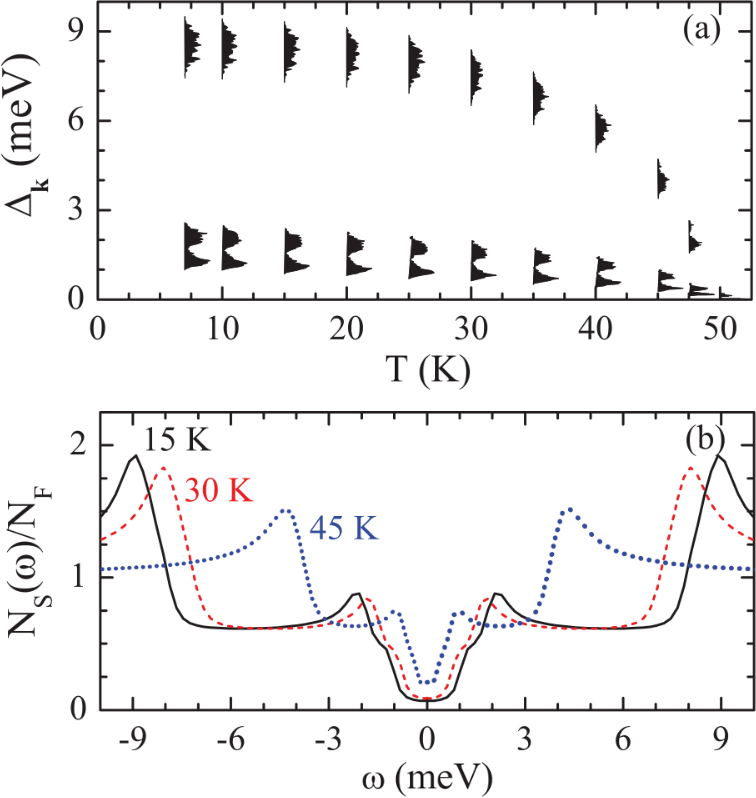
The first ab initio implementation of the anisotropic Migdal-Eliashberg theory was reported by Choi et al. (2002b, a) and Choi et al. (2003) in a study of the superconducting properties of MgB2. The authors succeeded to explain the anomalous heat capacity of MgB2 in terms of two distinct superconducting gaps, and obtained a in good agreement with experiment. These calculations were later extended to MgB2 under pressure Choi et al. (2009a) and other hypothetical borides Choi et al. (2009b). Margine and Giustino (2013) demonstrated an implementation of the Migdal-Eliashberg theory based on the Wannier interpolation scheme of Sec. VI, and reported applications to Pb and MgB2. The superconducting gap and superconducting density of states of MgB2 calculated by Margine and Giustino are shown in Fig. 17. In all these calculations, the Coulomb repulsion was described empirically via , and this partly accounts for the slight discrepancy between the calculated of 50 K and the experimental of 39 K Nagamatsu et al. (2001). Additional calculations based on the anisotropic Migdal-Eliashberg theory include a study of doped graphene Margine and Giustino (2014), as well as investigations of Li-decorated monolayer graphene Zheng and Margine (2016) and Ca-intercalated bilayer graphene Margine et al. (2016). In this latter work the authors incorporated Coulomb interactions from first principles, after calculating via the screened Coulomb interaction in the random-phase approximation. The calculated -8 K was in reasonable agreement with the experimental value of 4 K Ichinokura et al. (2016). The Migdal-Eliashberg theory has also been extended to describe the superconducting state as a function of applied magnetic field; a complete ab initio implementation was successfully demonstrated with an application to MgB2 Aperis et al. (2015). Very recently Sano et al. (2016) performed ab initio Migdal-Eliashberg calculations including retardation effects on high-pressure sulfur hydrides, obtaining good agreement with experiment. Interestingly in this work the authors also checked the effect of the zero-point renormalization of the electron bands within the Allen-Heine theory, and found that it accounts for a change in of up to 20 K.
XI.3 Density functional theory for superconductors
Another promising ab initio approach to the calculation of the superconducting critical temperature is the density functional theory for superconductors Lüders et al. (2005); Marques et al. (2005). The starting point of this approach is a generalization of the Hohenberg-Kohn theorem Hohenberg and Kohn (1964) to a system described by three densities: the electron density in the normal state, the density of superconducting pairs, and the nuclear density. Based on this premise, Lüders et al. mapped the fully-interacting system into an equivalent Kohn-Sham system Kohn and Sham (1965) of non-interacting nuclei and non-interacting, yet superconducting, electrons. The resulting Kohn-Sham equations for the electrons take the form of Bogoliubov-de Gennes equations Bogoliubov (1958), whereby electrons are paired by an effective gap function .
In its simplest formulation, the density functional theory for superconductors determines the expectation value of the pairing field over Kohn-Sham eigenstates, , using the following gap equation:
where . In this expression, the kernel contains information about the phonon-mediated pairing interaction and the Coulomb repulsion between electrons, , and contains information about the electron-phonon interaction. More specifically, and are evaluated starting from the electron-phonon matrix elements and the DFT electron band structure and phonon dispersions, as in the Migdal-Eliashberg theory. is approximated using the screened Coulomb interaction introduced below Eq. (207). Complete expressions for and can be found in Marques et al. (2005).

Equation (XI.3) is reminiscent of the gap equation in the Bardeen-Cooper-Schrieffer (BCS) theory Schrieffer (1983), with the difference that the ab initio kernel replaces the model interaction of the BCS theory, and the function introduces quasiparticle renormalization as in the Migdal-Eliashberg theory, see Eq. (208). At variance with the Migdal-Eliashberg theory, the gap function in the density functional theory for superconductors does not carry an explicity frequency dependence. Nevertheless, retardation effects are fully included through the dependence of the kernels and on the electron bands and the phonon dispersions. An important advantage of this theory is that the Coulomb potential is not required, since the electron-electron repulsion is seamlessly taken into account by means of the kernel .
The density functional theory for superconductors was successfully employed to study the superconducting properties of MgB2 Floris et al. (2005), Li, K, and Al under pressure Profeta et al. (2006); Sanna et al. (2006), Pb Floris et al. (2007), Ca-intercalated graphite Sanna et al. (2007), high-pressure hydrogen Cudazzo et al. (2008, 2010), CaBeSi Bersier et al. (2009), layered nitrides Akashi et al. (2012), alkali-doped fullerides Akashi and Arita (2013b), compressed sulfur hydrides Akashi et al. (2015), and intercalated layered carbides, silicides, and germanides Flores-Livas and Sanna (2015).
An interesting recent development of the theory was the determination of the superconducting order parameter in real space, Linscheid et al. (2015b). In the density functional theory for superconductors, the order parameter is obtained from the superconducting gap using the relation . Figure 18 shows the order parameter calculated by Linscheid et al. for both MgB2 and hole-doped graphane Savini et al. (2010). The plots show Friedel-like oscillations of the superconducting density as a function of the relative coordinates between two paired electrons.
XII Electron-phonon interactions beyond the local density approximation to DFT
The calculations of electron-phonon interactions reviewed in Sec. VII-XI have in common the fact that most investigations used the local density approximation to DFT or a generalized gradient approximation (GGA) such as the PBE functional Perdew et al. (1996a). Although the LDA and the GGA do represent the workhorse of electron-phonon calculations from first principles, there is growing evidence that these choices can lead to an underestimation of the electron-phonon coupling strength. At a conceptual level we can understand this point by rewriting the electron-phonon matrix element after combining Eqs. (38) and (142), (143):
| (212) |
In DFT the many-body dielectric matrix appearing in this expression is replaced by the RPA screening from Eq. (54). Given the DFT band gap problem, we expect to overestimate the screening, thereby leading to matrix elements which are underestimated to some extent.
Several groups investigated this point on quantitative grounds. Zhang et al. (2007) studied the electron-phonon coupling in a model copper oxide superconductor, CaCuO2. By calculating the vibrational frequencies of the half-breathing Cu-O stretching mode, the authors established that the local spin-density approximation (LSDA) yields phonons which are too soft (65.3 meV) as compared to experiment (80.1 meV). In contrast, the introduction of Hubbard corrections in a LSDA scheme restored agreement with experiment (80.9 meV). Since the electron-phonon matrix elements are connected to the phonon frequencies via the phonon self-energy, Eq. (145), a corresponding underestimation of the matrix elements can be expected. These results were supported by the work of Floris et al. (2011), who developed DFPT within LSDA, and applied their formalism to the phonon dispersions of antiferromagnetic MnO and NiO. Here the authors found that the DFT underestimates measured LO energies by as much as 15 meV in MnO, while the use of LSDA leads to good agreement with experiment. Related work was reported by Hong et al. (2012), who investigated the multiferroic perovskites CaMnO3, SrMnO3, BaMnO3, LaCrO3, LaFeO3, and the double perovskite La2CrFeO6. Here the authors calculated the variation of the vibrational frequencies between the ferromagnetic and the antiferromagnetic phases of these compounds as a function of the Hubbard parameter, and compared DFT calculations with hybrid-functional calculations.
Lazzeri et al. (2008) investigated the effect of quasiparticle corrections on the electron-phonon coupling of graphene and graphite, for the phonon at and the phonon at . They evaluated the intraband electron-phonon matrix elements using a frozen-phonon approach, noting that represents precisely the shift of the Kohn-Sham energy upon displacing the atoms according to the -th phonon eigenmode at . Lazzeri et al. found that the matrix elements increase by almost 40% from DFT to . The values led to slopes in the phonon dispersions near in very good agreement with inelastic X-ray scattering data Grüneis et al. (2009b). Similar results, albeit less dramatic, were obtained by Grüneis et al. (2009a) for the potassium-intercalated graphite KC8.
Laflamme Janssen et al. (2010) studied the electron-phonon coupling in the C60 molecule as a model for superconducting alkali-doped fullerides. They employed the PBE0 hybrid functional Perdew et al. (1996b) with a fraction of exact exchange %, and obtained an enhancement of the total coupling strength of 42% as compared to PBE. This work was followed up by Faber et al. (2011), who used the approximation and obtained a similar enhancement of 48%. We also point out an earlier work by Saito (2002) based on the B3LYP functional, reporting similar results.
Yin et al. (2013) investigated the effects of using the approximation and the HSE hybrid functional Heyd et al. (2003) on the electron-phonon coupling in the superconducting bismuthates Ba1-xKxBiO3 and chloronitrides -ZrNCl, as well as MgB2. In the case of Ba1-xKxBiO3 the authors obtained a three-fold increase in the coupling strength from PBE to HSE. This enhancement brought the critical temperature calculated using Eq. (204) to 31 K, very close to the experimental value of 32 K. Similarly, in the case of -ZrNCl, Yin et al. obtained a 50% increase of , bringing the calculated critical temperature, 18 K, close to the experimental value of 16 K. Instead, in the case of MgB2, they noticed only a slight increase of the electron-phonon coupling as compared to the standard LDA.
Another application of hybrid functionals to the study of EPIs was reported by Komelj and Krakauer (2015). Here the authors investigated the sensitivity of the superconducting critical temperature of the H3S phase of sulfur hydride to the exchange and correlation functional. They found that the PBE0 functional enhances the critical temperature by up to 25% as compared to PBE, bringing from 201-217 K to 253-270 K (the spread in values is related to the choice of the parameter ).
Mandal et al. (2014) reported work on the superconductor FeSe based on dynamical mean-field theory (DMFT). In this case DMFT yielded a three-fold enhancement of the coupling strength for selected modes.
As already mentioned in Sec. IX.1.1, Antonius et al. (2014) performed calculations of the electron-phonon coupling in diamond using a frozen-phonon approach. They found that quasiparticle corrections lead to a uniform enhancement of the electron-phonon matrix elements. The net effect is an increase of the zero-point renormalization of the band gap by 40% as compared to standard LDA calculations. Monserrat (2016a) confirmed this result and found a correction of comparable magnitude in the case of silicon. However, Monserrat also found that the corrections to the zero-point band gap renormalization of LiF, MgO, and TiO2 are very small (5% of the PBE value), therefore at present it is not possible to draw general conclusions.
Finally, we mention that Faber et al. (2015) examined possible strategies for systematically incorporating corrections in electron-phonon calculations. By using diamond, graphene, and C60 as test cases, the authors showed that a ‘constant screening’ approximation is able to reproduce complete results with an error below 10% at reduced computational cost. This approximation amounts to evaluating the variation of the Green’s function in a frozen-phonon calculation, while retaining the screened Coulomb interaction of the unperturbed ground state.
All these recent developments point to the need of moving beyond local exchange and correlation functionals in the study of electron-phonon interactions from first principles. In the future, it will be important to devise accurate computational methods for calculating not only the intraband electron-phonon matrix elements (as in the frozen-phonon method) but also matrix elements between all states and for scattering across the entire Brillouin zone.
For the sake of completeness we emphasize that the underestimation of the EPI matrix elements by semilocal DFT functionals does not propagate in the same way into different materials properties. This is readily understood by examining two fundamental quantities, the Allen-Heine renormalization of electron bands, Eq. (167), and the adiabatic phonon frequencies, as obtained from Eqs. (126) and (127). In the former case the electronic screening enters as ; in the latter case the screening contributes through a term which scales with . As a result, in the hypothetical case of a semiconductor for which DFT underestimated the electronic permittivity by 20%, we would have an error of 40% in the energy renormalization, and of 10% in the phonon frequencies. This example is an oversimplification of the problem, but it shows that different properties relating to the EPI could be affected to a very different degree by the inherent limitations of DFT functionals.
XIII Conclusions
The study of electron-phonon interactions has a long and distinguished history, but it is only during the past two decades that quantitative and predictive calculations have become possible. First-principles calculations of electron-phonon couplings are finding an unprecedented variety of applications in many areas of condensed matter and materials physics, from spectroscopy to transport, from metals to semiconductors and superconductors. In this article we discussed the standard DFT formalism for performing calculations of electron-phonon interactions, we showed how most equations can be derived from a field-theoretic framework using a few well-defined approximations, and we reviewed recent applications of the theory to many materials of current interest.
As calculation methods improve relentlessly and quantitative comparisons between theory and experiment become increasingly refined, new and more complex questions arise. Much is still left to do, both in the fundamental theory of electron-phonon interactions, and in the development of more accurate and more efficient computational methods.
For one, we are still using theories where the coupling matrix elements are calculated using the adiabatic local density approximation to DFT. The need for moving beyond standard DFT and beyond the adiabatic approximation can hardly be overemphasized. Progress is being made on the incorporation of nonlocal corrections into electron-phonon matrix elements, for example using hybrid functionals or techniques, but very little is known about retardation effects. It is expected that such effects may be important in the study of heavily doped oxides and semiconductors, both in their normal and superconducting states (Mahan, 1993, Sec. 6.3.A), but ab initio investigations are currently missing. This is truly uncharted territory and a systematic effort in this direction is warranted.
In this article we emphasized that it is possible to formulate a compact, unified theory of electron-phonon interactions starting from a fully ab initio field-theoretic approach. The only assumption which is absolutely crucial to the theory is the harmonic approximation. Abandoning the harmonic approximation leads to the appearance of several new terms in the equations, and the resulting formalism becomes considerably more complex than in Table 1. Despite these difficulties, given the importance of anharmonic effects in many systems of current interest, extending the theory to the case of anharmonic phonons and multi-phonon interactions constitutes a pressing challenge. Ab initio investigations of anharmonic effects on the temperature dependence of band gaps have recently been reported (Monserrat et al., 2013; Antonius et al., 2015). Since these studies rely on non-perturbative adiabatic calculations in supercells, it would be highly desirable to establish a clear formal connection of these methods with the rigorous field-theoretic approach of Sec. IV. Along the same line, it would be important to clarify the relation between many-body approaches, adiabatic supercells calculations, and more traditional classical or path-integral molecular dynamics simulations.
The study of electron-phonon interactions has long been dominated by Fröhlich-like Hamiltonians, whereby the electron-phonon coupling is retained only to linear order in the atomic displacements. This is the case for all the model Hamiltonians mentioned in Sec. V.2.6. It is now clear that quadratic couplings, leading to the Debye-Waller contributions in the optical spectra of semiconductors, are by no means negligible and should be investigated more systematically. For example, in the current literature it is invariably assumed that Debye-Waller contributions are negligible in metals near the Fermi surface; while this is probably the case for the simplest elemental metals, what happens in the case of multiple Fermi-surface sheets is far from clear, and should be tested by direct calculations.
The identification of the correct matrix elements to be calculated is not always a trivial task, as it was discussed for the case of the non-adiabatic phonon self-energy. In the future it will be important to pay attention to these aspects, especially in view of detailed comparison with experiment. For now, the issue on whether the phonon self-energy arising from EPIs should be calculated using bare or screened EPI matrix elements (Sec. VII) is to be considered an open question, and calls for further investigation.
The theory and applications reviewed in this article focused on non-magnetic systems. The rationale for this choice is that a complete many-body theory of electron-phonon interactions for magnetic systems is not available yet. Recent investigations of spin-phonon couplings were conducted by assuming that the spin and the vibrational degrees of freedom can be decoupled, as in the Born-Oppenheimer approximation. Under this assumption it is possible to investigate how the spin configuration responds to a frozen phonon, or alternatively how the vibrational frequencies depend on the spin configuration (see for example Chan et al., 2007; Łażewski et al., 2010; Lee and Rabe, 2011; Cao et al., 2015). In all these cases it would be desirable to employ a more rigorous many-body theory of spin-phonon interactions. The Hedin-Baym equations discussed in Sec. IV maintain their validity in the case of spin-polarized systems, provided collinear spins are assumed. In more general situations, where it is important to consider noncollinear spins, external magnetic perturbations, or spin-dependent interactions such as spin-orbit and Rashba-Dresselhaus couplings, it becomes necessary to generalize the equations in Table 1. Although such a generalization has not been reported yet, the work of Aryasetiawan and Biermann (2008) constitutes a promising starting point. In that work the Schwinger functional derivative technique (see Sec. IV.2.1) was used to extend Hedin’s equations at clamped nuclei to systems containing spin-dependent interactions. Generalizing Aryasetiawan and Biermann’s work to incorporate nuclear vibrations will be important for the study of electron-phonon interactions in many systems of current interest, from multifunctional materials to topological quantum matter.
At this time it is not possible to predict how this fast-moving field will evolve over the years to come. However, the impressive progress made during the past decade gives us confidence that this interesting research area will continue to thrive, and will keep surprising us with fascinating challenges and exciting new opportunities.
Acknowledgements.
I am indebted with Samuel Poncé, Carla Verdi, and Marios Zacharias for a critical reading of the manuscript, and with many colleagues who have kindly provided feedback on the arXiv preprint version of this article. This article is the result of many stimulating discussions with friends and colleagues over the last few years. I would like to thank in particular Philip Allen, Stefano Baroni, Lilia Boeri, Nicola Bonini, Fabio Caruso, Hyoung Joon Choi, Marvin Cohen, Michel Côté, Andrea Dal Corso, Claudia Draxl, Asier Eiguren, Giulia Galli, Paolo Giannozzi, Stefano de Gironcoli, Xavier Gonze, Göran Grimvall, Eberhard Gross, Branko Gumhalter, Sohrab Ismail-Beigi, Emmanuil Kioupakis, Georg Kresse, Steven Louie, Roxana Margine, Andrea Marini, Miguel Marques, Nicola Marzari, Takashi Miyake, Bartomeu Monserrat, Jeffrey Neaton, Richard Needs, Jesse Noffsinger, Cheol-Hwan Park, Christopher Patrick, Warren Pickett, Samuel Poncé, Paolo Radaelli, Lucia Reining, John Rehr, Patrick Rinke, Angel Rubio, Matthias Scheffler, Young-Woo Son, Alexander Tkatchenko, Chris Van de Walle, Carla Verdi, Matthieu Verstraete, and Marios Zacharias. I also would like to thank Marco Bernardi, Asier Eiguren, Xavier Gonze, Eberhard Gross, Wu Li, Steven Louie, and Francesco Mauri for kindly allowing me to reproduce their figures. This work was supported by the Leverhulme Trust (Grant RL-2012-001), the Graphene Flagship (Horizon 2020 grant no. 696656-GrapheneCore1), and the UK Engineering and Physical Sciences Research Council (Grants No. EP/J009857/1 and No. EP/M020517/1).Appendix A Born-von Kármán boundary conditions
In this Appendix we provide more details on the notation related to the Born-von Kármán boundary conditions used throughout this article. The crystalline unit cell is defined by the primitive lattice vectors with , and the -th unit cell is identified by the vector with integers between 0 and . The BvK supercell contains unit cells. The primitive vectors of the reciprocal lattice are denoted by , and fulfil the duality condition . We consider Bloch wavevectors belonging to a uniform grid in one unit cell of the reciprocal lattice: with being integers between 0 and . This grid contains the same number of -vectors as the number of unit cells in the BvK supercell. From these definitions the standard sum rules follow:
| (213) |
If is a reciprocal-lattice vector, the replacement of any of the -vectors by in these expressions and in all expressions presented in this article is inconsequential, since . Similarly any replacement of by where is a lattice vectors of the BvK supercell is inconsequential. Owing to these properties we are at liberty to replace the -grid defined above with a Wigner-Seitz grid, i.e. the first Brillouin zone, and the supercell with a Wigner-Seitz supercell. These choices are useful for practical calculations in order to exploit the symmetry operations of the crystal, and to truncate the interatomic force constants, given by Eq. (13), outside a Wigner-Seitz supercell.
Appendix B Ladder operators in extended systems
In this Appendix we describe the construction of the phonon ladder operators , and derive the phonon Hamiltonian given by Eq. (22). We show how the definition of the ladder operators depends on the behavior of the wavevector under inversion.
The normal modes introduced in Eq. (15) can be used to define a linear coordinate transformation of the ionic displacements as follows:
| (214) |
Here is referred to as ‘complex normal coordinate’ Brüesch (1982). The exponential and the masses in Eq. (214) are chosen so as to obtain Eq. (22) starting from Eq. (12). Since there are degrees of freedom, and since the complex normal coordinates correspond to real variables, this coordinate transformation carries some redundancy. Indeed by combining Eqs. (18) and (214) it is seen that:
| (215) |
The inverse relation of Eq. (214) is:
| (216) |
The right-hand side is real-valued after Eqs. (18) and (215). In preparation for the transition to a quantum description of lattice vibrations, it is useful to identify independent normal coordinates. This can be done by partitioning the grid of -vectors in three sets. We call the set of vectors which are invariant under inversion, that is for some reciprocal lattice vector (including ). The center of the Brillouin zone and the centers of its faces belong to this set. The remaining vectors can be separated further in and , in such a way that all the vectors in are obtained from those in by inversion (modulo a reciprocal lattice vector). After defining , Eq. (216) can be rewritten as:
| (217) | |||||
The -vectors of the set have been grouped together with those in by taking the real part in the second line. It can be verified that in this expression there are exactly real coordinates, therefore we can choose the for in and the pairs , for in as the independent variables. These variables are referred to as ‘real normal coordinates’ Brüesch (1982).
Using Eqs. (12)-(18), (213), and (217) the nuclear Hamiltonian can be written in terms of independent harmonic oscillators in the real normal coordinates:
| (218) | |||||
where for ease of notation we performed the scaling:
| (219) | |||||
| (220) |
with being the zero-point displacement amplitude of Eq. (21). In the case of there are three normal modes for which , and the corresponding potential terms must be removed from Eq. (218).
The eigenstates of Eq. (218) are found by introducing the real ladder operators for each normal coordinate Cohen-Tannoudji et al. (1977):
| (221) |
and similarly for . With these definitions Eq. (218) becomes:
| (222) | |||||
The eigenstates of this Hamiltonian are products of simple harmonic oscillators Merzbacher (1998), and the ground state is:
| (223) |
with a normalization constant. The relations between the positions and the normal coordinates , are given by Eqs. (214), (219)-(220), and (21).
The eigenstates of can be generated by applying and to the ground state . However this approach is not entirely satisfactory, since we cannot assign separate quantum numbers to modes with wavevectors or . In order to avoid this inconvenience we observe that, for each normal mode, the first line of Eq. (218) defines an effective isotropic two-dimensional harmonic oscillator. The degenerate eigenstates of this oscillator can be combined to form eigenstates of the angular momentum; this leads to right and left circular quanta with the same energy and definite angular momentum Cohen-Tannoudji et al. (1977). This analogy motivates the consideration of the following linear combinations, for in :
| (224) | |||||
| (225) |
Since both and lower the energy of an eigenstate by the same quantum of energy , the resulting states are degenerate and their linear combinations are also eigenstates for the same eigenvalue. As a consequence we can generate all the eigenstates of the Hamiltonian by acting on the ground state with the creation operators and . In this reasoning the wavevectors belong to ; if we now consider Eqs. (215), (224), and (225) we see that formally we also have . Therefore it is natural to associate to phonons propagating along the direction .
These observations suggest replacing the real ladder operators of Eq. (221) by the complex ladder operators and for in and , respectively. In the case of in we keep the real operators . These definitions can be turned into the compact expressions:
| (226) | |||||
| (227) |
Using these operators the nuclear Hamiltonian of Eq. (218) takes the well-known form given by Eq. (22). Any eigenstate of can now be generated as . In this form we see that it is possible to assign independently a number of phonons to each wavevector and each mode . Using Eqs. (219)-(221) and (226)-(227) we also have the basic identity:
| (228) |
By combining this last expression with Eq. (216) we obtain Eq. (20).
References
- Abrikosov et al. (1975) Abrikosov, A A, L. P. Gor’kov, and I. E. Dzyaloshinski (1975), Methods of Quantum Field Theory in Statistical Physics (Dover).
- Adler (1962) Adler, S L (1962), “Quantum theory of the dielectric constant in real solids,” Phys. Rev. 126, 413–420.
- Agapito et al. (2013) Agapito, L A, A. Ferretti, A. Calzolari, S. Curtarolo, and M. Buongiorno Nardelli (2013), “Effective and accurate representation of extended Bloch states on finite Hilbert spaces,” Phys. Rev. B 88, 165127.
- Akashi and Arita (2013a) Akashi, R, and R. Arita (2013a), “Development of density-functional theory for a plasmon-assisted superconducting state: Application to lithium under high pressures,” Phys. Rev. Lett. 111, 057006.
- Akashi and Arita (2013b) Akashi, R, and R. Arita (2013b), “Nonempirical study of superconductivity in alkali-doped fullerides based on density functional theory for superconductors,” Phys. Rev. B 88, 054510.
- Akashi et al. (2015) Akashi, R, M. Kawamura, S. Tsuneyuki, Y. Nomura, and R. Arita (2015), “First-principles study of the pressure and crystal-structure dependences of the superconducting transition temperature in compressed sulfur hydrides,” Phys. Rev. B 91, 224513.
- Akashi et al. (2012) Akashi, R, K. Nakamura, R. Arita, and M. Imada (2012), “High-temperature superconductivity in layered nitrides -LiNCl ( Ti, Zr, Hf): Insights from density functional theory for superconductors,” Phys. Rev. B 86, 054513.
- Albers et al. (1976) Albers, R C, L. Bohlin, M. Roy, and J. W. Wilkins (1976), “Normal and umklapp phonon decay rates due to phonon-phonon and electron-phonon scattering in potassium at low temperatures,” Phys. Rev. B 13, 768–786.
- Alexandrov (2008) Alexandrov, A S (2008), Polarons in advanced materials (Springer).
- Alexandrov and Devreese (2010) Alexandrov, A S, and J. T. Devreese (2010), Advances in polaron physics (Springer).
- Allen (1972a) Allen, P B (1972a), “Electron-phonon coupling and pseudopotentials: The mass enhancements of the noble metals,” Phys. Rev. B 5, 3857–3862.
- Allen (1972b) Allen, P B (1972b), “Neutron spectroscopy of superconductors,” Phys. Rev. B 6, 2577–2579.
- Allen (1976) Allen, P B (1976), “Fermi-surface harmonics: A general method for nonspherical problems. application to Boltzmann and Eliashberg equations,” Phys. Rev. B 13, 1416–1427.
- Allen (1978) Allen, P B (1978), “Solids with thermal or static disorder. I. one-electron properties,” Phys. Rev. B 18, 5217–5224.
- Allen and Cardona (1981) Allen, P B, and M. Cardona (1981), “Theory of the temperature dependence of the direct gap of germanium,” Phys. Rev. B 23, 1495–1505.
- Allen and Cardona (1983) Allen, P B, and M. Cardona (1983), “Temperature dependence of the direct gap of Si and Ge,” Phys. Rev. B 27, 4760–4769.
- Allen and Cohen (1969) Allen, P B, and M. L. Cohen (1969), “Pseudopotential calculation of the mass enhancement and superconducting transition temperature of simple metals,” Phys. Rev. 187, 525–538.
- Allen and Cohen (1970) Allen, P B, and M. L. Cohen (1970), “Calculation of the temperature dependence of the electron-phonon mass enhancement,” Phys. Rev. B 1, 1329–1336.
- Allen et al. (1968) Allen, P B, M. L. Cohen, L. M. Falicov, and R. V. Kasowski (1968), “Superconductivity and band structure from a single pseudopotential: Zinc and cadmium,” Phys. Rev. Lett. 21, 1794–1796.
- Allen and Dynes (1975) Allen, P B, and R. C. Dynes (1975), “Transition temperature of strong-coupled superconductors reanalyzed,” Phys. Rev. B 12, 905–922.
- Allen and Heine (1976) Allen, P B, and V. Heine (1976), “Theory of the temperature dependence of electronic band structures,” J. Phys. C 9, 2305.
- Allen and Hui (1980) Allen, P B, and J. C. K. Hui (1980), “Thermodynamics of solids: Corrections from electron-phonon interactions,” Z. Phys. B 37, 33–38.
- Allen and Lee (1972) Allen, P B, and M. J. G. Lee (1972), “Phase-shift pseudopotentials and the electron-phonon interaction: Theory and results for alkali metals,” Phys. Rev. B 5, 3848–3857.
- Allen and Mitrovic (1982) Allen, P B, and B. Mitrovic (1982), Theory of Superconducting , edited by F. Seitz, D. Turnbull, and H. Ehrenreich, Solid State Physics, Vol. 37 (Academic).
- Allen and Nery (2017) Allen, P B, and J. P. Nery (2017), “Low-temperature semiconductor band-gap thermal shifts: shifts from ordinary acoustic and from piezoacoustic coupling,” Phys. Rev. B 95, 035211.
- Animalu and Heine (1965) Animalu, A O E, and V. Heine (1965), “The screened model potential for 25 elements,” Phil. Mag. 12, 1249–1270.
- Antonc̆ík (1955) Antonc̆ík, E (1955), “On the theory of temperature shift of the absorption curve in non-polar crystals,” Czech. J. Phys. 5, 449–461.
- Antonius et al. (2014) Antonius, G, S. Poncé, P. Boulanger, M. Côté, and X. Gonze (2014), “Many-body effects on the zero-point renormalization of the band structure,” Phys. Rev. Lett. 112, 215501.
- Antonius et al. (2015) Antonius, G, S. Poncé, E. Lantagne-Hurtubise, G. Auclair, X. Gonze, and M. Côté (2015), “Dynamical and anharmonic effects on the electron-phonon coupling and the zero-point renormalization of the electronic structure,” Phys. Rev. B 92, 085137.
- Aperis et al. (2015) Aperis, A, P. Maldonado, and P. M. Oppeneer (2015), “Ab initio theory of magnetic-field-induced odd-frequency two-band superconductivity in mgb2,” Phys. Rev. B 92, 054516.
- Aryasetiawan and Biermann (2008) Aryasetiawan, F, and S. Biermann (2008), “Generalized hedin’s equations for quantum many-body systems with spin-dependent interactions,” Phys. Rev. Lett. 100, 116402.
- Aryasetiawan and Gunnarsson (1998) Aryasetiawan, F, and O. Gunnarsson (1998), “The method,” Rep. Prog. Phys. 61, 237.
- Aryasetiawan et al. (1996) Aryasetiawan, F, L. Hedin, and K. Karlsson (1996), “Multiple plasmon satellites in Na and Al spectral functions from ab initio cumulant expansion,” Phys. Rev. Lett. 77, 2268–2271.
- Ashcroft and Mermin (1976) Ashcroft, N W, and N. D. Mermin (1976), Solid state physics (Harcourt, New York).
- Ashcroft and Wilkins (1965) Ashcroft, N W, and J. W. Wilkins (1965), “Low temperature electronic specific heat of simple metals,” Phys. Lett. 14, 285–287.
- Audouze et al. (2006) Audouze, C, F. Jollet, M. Torrent, and X. Gonze (2006), “Projector augmented-wave approach to density-functional perturbation theory,” Phys. Rev. B 73, 235101.
- Bachelet et al. (1982) Bachelet, G B, D. R. Hamann, and M. Schlüter (1982), “Pseudopotentials that work: From H to Pu,” Phys. Rev. B 26, 4199–4228.
- Bardeen (1937) Bardeen, J (1937), “Conductivity of monovalent metals,” Phys. Rev. 52, 688–697.
- Bardeen and Pines (1955) Bardeen, J, and D. Pines (1955), “Electron-phonon interaction in metals,” Phys. Rev. 99, 1140–1150.
- Bardeen and Shockley (1950) Bardeen, J, and W. Shockley (1950), “Deformation potentials and mobilities in non-polar crystals,” Phys. Rev. 80, 72–80.
- Baroni et al. (1987) Baroni, S, P. Giannozzi, and A. Testa (1987), “Green’s-function approach to linear response in solids,” Phys. Rev. Lett. 58, 1861–1864.
- Baroni et al. (2001) Baroni, S, S. de Gironcoli, A. Dal Corso, and P. Giannozzi (2001), “Phonons and related crystal properties from density-functional perturbation theory,” Rev. Mod. Phys. 73, 515–562.
- von Barth and Hedin (1972) von Barth, U, and L. Hedin (1972), “A local exchange-correlation potential for the spin polarized case. I,” J. Phys. C 5, 1629.
- Bassani and Parravicini (1975) Bassani, G F, and G. P. Parravicini (1975), Electronic states and optical transitions in solids (Pergamon).
- Bauer et al. (1998) Bauer, R, A. Schmid, P. Pavone, and D. Strauch (1998), “Electron-phonon coupling in the metallic elements Al, Au, Na, and Nb: A first-principles study,” Phys. Rev. B 57, 11276–11282.
- Baym (1961) Baym, G (1961), “Field-theoretic approach to the properties of the solid state,” Ann. Phys. 14, 1–42.
- Becker and Fan (1949) Becker, M, and H. Y. Fan (1949), “Optical properties of semiconductors. III. infra-red transmission of silicon,” Phys. Rev. 76, 1531–1532.
- Berciu (2006) Berciu, M (2006), “Green’s function of a dressed particle,” Phys. Rev. Lett. 97, 036402.
- Berger et al. (1995) Berger, E, P. Valášek, and W. von der Linden (1995), “Two-dimensional Hubbard-Holstein model,” Phys. Rev. B 52, 4806–4814.
- Bernardi et al. (2014) Bernardi, M, D. Vigil-Fowler, J. Lischner, J. B. Neaton, and S. G. Louie (2014), “Ab initio study of hot carriers in the first picosecond after sunlight absorption in silicon,” Phys. Rev. Lett. 112, 257402.
- Bernardi et al. (2015) Bernardi, M, D. Vigil-Fowler, C. S. Ong, J. B. Neaton, and S. G. Louie (2015), “Ab initio study of hot electrons in GaAs,” Proc. Natl. Acad. Sci. 112, 5291–5296.
- Bersier et al. (2009) Bersier, C, A. Floris, A. Sanna, G. Profeta, A. Continenza, E. K. U. Gross, and S. Massidda (2009), “Electronic, vibrational, and superconducting properties of CaBeSi: First-principles calculations,” Phys. Rev. B 79, 104503.
- Bhosale et al. (2012) Bhosale, J, A. K. Ramdas, A. Burger, A. Muñoz, A. H. Romero, M. Cardona, R. Lauck, and R. K. Kremer (2012), “Temperature dependence of band gaps in semiconductors: Electron-phonon interaction,” Phys. Rev. B 86, 195208.
- Bianchi et al. (2010) Bianchi, M, E. D. L. Rienks, S. Lizzit, A. Baraldi, R. Balog, L. Hornekær, and Ph. Hofmann (2010), “Electron-phonon coupling in potassium-doped graphene: Angle-resolved photoemission spectroscopy,” Phys. Rev. B 81, 041403.
- Bloch (1929) Bloch, F (1929), “Über die Quantenmechanik der Elektronen in Kristallgittern,” Z. Phys. 52, 555–600.
- Blöchl (1994) Blöchl, P E (1994), “Projector augmented-wave method,” Phys. Rev. B 50, 17953–17979.
- Bogoliubov (1958) Bogoliubov, N N (1958), “A new method in the theory of superconductivity. I,” Sov. Phys. JETP 7, 41–46.
- Bonini et al. (2007) Bonini, N, M. Lazzeri, N. Marzari, and F. Mauri (2007), “Phonon anharmonicities in graphite and graphene,” Phys. Rev. Lett. 99, 176802.
- Born and Huang (1954) Born, M, and K. Huang (1954), Dynamical Theory of Crystal Lattices (Clarendon).
- Born and Oppenheimer (1927) Born, M, and R. Oppenheimer (1927), “Zur Quantentheorie der Molekeln,” Ann. Phys. 389, 457–484.
- Borysenko et al. (2010) Borysenko, K M, J. T. Mullen, E. A. Barry, S. Paul, Y. G. Semenov, J. M. Zavada, M. Buongiorno Nardelli, and K. W. Kim (2010), “First-principles analysis of electron-phonon interactions in graphene,” Phys. Rev. B 81, 121412.
- Bostwick et al. (2007) Bostwick, A, T. Ohta, T. Seyller, K. Horn, and E. Rotenberg (2007), “Quasiparticle dynamics in graphene,” Nat. Phys. 3, 36–40.
- Botti and Marques (2013) Botti, S, and M. A. L. Marques (2013), “Strong renormalization of the electronic band gap due to lattice polarization in the formalism,” Phys. Rev. Lett. 110, 226404.
- Broido et al. (2007) Broido, D A, M. Malorny, G. Birner, N. Mingo, and D. A. Stewart (2007), “Intrinsic lattice thermal conductivity of semiconductors from first principles,” Appl. Phys. Lett. 91, 231922.
- Brouder et al. (2007) Brouder, C, G. Panati, M. Calandra, C. Mourougane, and N. Marzari (2007), “Exponential localization of Wannier functions in insulators,” Phys. Rev. Lett. 98, 046402.
- Brüesch (1982) Brüesch, P (1982), Phonons, Theory and Experiments, v. 1 (Springer-Verlag).
- Bungaro et al. (2000) Bungaro, C, K. Rapcewicz, and J. Bernholc (2000), “Ab initio phonon dispersions of wurtzite AlN, GaN, and InN,” Phys. Rev. B 61, 6720–6725.
- Butler et al. (1979) Butler, W H, F. J. Pinski, and P. B. Allen (1979), “Phonon linewidths and electron-phonon interaction in Nb,” Phys. Rev. B 19, 3708–3721.
- Calandra and Mauri (2007) Calandra, M, and F. Mauri (2007), “Electron-phonon coupling and electron self-energy in electron-doped graphene: Calculation of angular-resolved photoemission spectra,” Phys. Rev. B 76, 205411.
- Calandra et al. (2010) Calandra, M, G. Profeta, and F. Mauri (2010), “Adiabatic and nonadiabatic phonon dispersion in a Wannier function approach,” Phys. Rev. B 82, 165111.
- Campbell et al. (1984) Campbell, D K, T. A. DeGrand, and S. Mazumdar (1984), “Soliton energetics in Peierls-Hubbard models,” Phys. Rev. Lett. 52, 1717–1720.
- Cancellieri et al. (2016) Cancellieri, C, A. S. Mishchenko, U. Aschauer, A. Filippetti, C. Faber, O. S. Barišić, V. A. Rogalev, T. Schmitt, N. Nagaosa, and V. N. Strocov (2016), “Polaronic metal state at the LaAlO3/SrTiO3 interface,” Nat. Commun. 7, 10386.
- Cannuccia and Marini (2011) Cannuccia, E, and A. Marini (2011), “Effect of the quantum zero-point atomic motion on the optical and electronic properties of diamond and trans-polyacetylene,” Phys. Rev. Lett. 107, 255501.
- Cannuccia and Marini (2012) Cannuccia, E, and A. Marini (2012), “Zero point motion effect on the electronic properties of diamond, trans-polyacetylene and polyethylene,” Eur. Phys. J. B 85, 320.
- Cannuccia and Marini (2013) Cannuccia, E, and A. Marini (2013), “Ab initio study of the effects induced by the electron-phonon scattering in carbon based nanostructures,” arXiv1304.0072 .
- Cao et al. (2015) Cao, K, F. Giustino, and P. G. Radaelli (2015), “Theory of electromagnons in CuO,” Phys. Rev. Lett. 114, 197201.
- Capaz et al. (2005) Capaz, R B, C. D. Spataru, P. Tangney, M. L. Cohen, and S. G. Louie (2005), “Temperature dependence of the band gap of semiconducting carbon nanotubes,” Phys. Rev. Lett. 94, 036801.
- Carbotte and Dynes (1967) Carbotte, J P, and R. C. Dynes (1967), “Resistivity of solid aluminum,” Phys. Lett. A 25, 532–533.
- Cardona (2001) Cardona, M (2001), “Renormalization of the optical response of semiconductors by electron-phonon interaction,” Phys. Status Solidi A 188, 1209–1232.
- Cardona (2005) Cardona, M (2005), “Electron-phonon interaction in tetrahedral semiconductors,” Solid State Commun. 133, 3–18.
- Cardona and Thewalt (2005) Cardona, M, and M. L. W. Thewalt (2005), “Isotope effects on the optical spectra of semiconductors,” Rev. Mod. Phys. 77, 1173–1224.
- Caruso and Giustino (2015) Caruso, F, and F. Giustino (2015), “Spectral fingerprints of electron-plasmon coupling,” Phys. Rev. B 92, 045123.
- Caruso et al. (2015) Caruso, F, H. Lambert, and F. Giustino (2015), “Band structures of plasmonic polarons,” Phys. Rev. Lett. 114, 146404.
- Caudal et al. (2007) Caudal, N, A. M. Saitta, M. Lazzeri, and F. Mauri (2007), “Kohn anomalies and nonadiabaticity in doped carbon nanotubes,” Phys. Rev. B 75, 115423.
- Ceperley and Alder (1980) Ceperley, D M, and B. J. Alder (1980), “Ground state of the electron gas by a stochastic method,” Phys. Rev. Lett. 45, 566–569.
- Chakraborty and Allen (1978) Chakraborty, B, and P. B. Allen (1978), “Theory of temperature dependence of optical properties of solids,” J. Phys. C 11, L9.
- Chan et al. (2007) Chan, K T, J. D. Sau, P. Zhang, and M. L. Cohen (2007), “Ab initio calculations of phonon splitting in antiferromagnetic ZnCr2O4,” Phys. Rev. B 75, 054304.
- Chang and Cohen (1986) Chang, K J, and M. L. Cohen (1986), “Electron-phonon interactions and superconductivity in Si, Ge, and Sn,” Phys. Rev. B 34, 4552–4557.
- Chang et al. (1985) Chang, K J, M. M. Dacorogna, M. L. Cohen, J. M. Mignot, G. Chouteau, and G. Martinez (1985), “Superconductivity in high-pressure metallic phases of Si,” Phys. Rev. Lett. 54, 2375–2378.
- Chen et al. (2015) Chen, C, J. Avila, E. Frantzeskakis, A. Levy, and M. C Asensio (2015), “Observation of a two-dimensional liquid of Fröhlich polarons at the bare SrTiO3 surface,” Nat. Commun. 6, 8585.
- Choi et al. (2003) Choi, H J, M. L. Cohen, and S. G. Louie (2003), “Anisotropic Eliashberg theory of MgB2: , isotope effects, superconducting energy gaps, quasiparticles, and specific heat,” Physica C 385, 66–74.
- Choi et al. (2009a) Choi, H J, S. G. Louie, and M. L. Cohen (2009a), “Anisotropic Eliashberg theory for superconductivity in compressed and doped ,” Phys. Rev. B 79, 094518.
- Choi et al. (2009b) Choi, H J, S. G. Louie, and M. L. Cohen (2009b), “Prediction of superconducting properties of using anisotropic Eliashberg theory,” Phys. Rev. B 80, 064503.
- Choi et al. (2002a) Choi, H J, D. Roundy, H. Sun, M. L. Cohen, and S. G. Louie (2002a), “First-principles calculation of the superconducting transition in MgB2 within the anisotropic Eliashberg formalism,” Phys. Rev. B 66, 020513.
- Choi et al. (2002b) Choi, H J, D. Roundy, H. Sun, M. L. Cohen, and S. G. Louie (2002b), “The origin of the anomalous superconducting properties of MgB2,” Nature 418, 758–760.
- Cohen and Heine (1961) Cohen, M H, and V. Heine (1961), “Cancellation of kinetic and potential energy in atoms, molecules, and solids,” Phys. Rev. 122, 1821–1826.
- Cohen and Bergstresser (1966) Cohen, M L, and T. K. Bergstresser (1966), “Band structures and pseudopotential form factors for fourteen semiconductors of the diamond and zinc-blende structures,” Phys. Rev. 141, 789–796.
- Cohen-Tannoudji et al. (1977) Cohen-Tannoudji, C, B. Diu, and F. Laloe (1977), Quantum Mechanics, v. 1 (Wiley).
- Cowley (1963) Cowley, R A (1963), “The lattice dynamics of an anharmonic crystal,” Adv. Phys. 12, 421–480.
- Cudazzo et al. (2008) Cudazzo, P, G. Profeta, A. Sanna, A. Floris, A. Continenza, S. Massidda, and E. K. U. Gross (2008), “Ab Initio description of high-temperature superconductivity in dense molecular hydrogen,” Phys. Rev. Lett. 100, 257001.
- Cudazzo et al. (2010) Cudazzo, P, G. Profeta, A. Sanna, A. Floris, A. Continenza, S. Massidda, and E. K. U. Gross (2010), “Electron-phonon interaction and superconductivity in metallic molecular hydrogen. II. superconductivity under pressure,” Phys. Rev. B 81, 134506.
- Dacorogna et al. (1985a) Dacorogna, M M, K. J. Chang, and M. L. Cohen (1985a), “Pressure increase of the electron-phonon interaction in superconducting hexagonal silicon,” Phys. Rev. B 32, 1853–1855.
- Dacorogna et al. (1985b) Dacorogna, M M, M. L. Cohen, and P. K. Lam (1985b), “Self-consistent calculation of the q dependence of the electron-phonon coupling in aluminum,” Phys. Rev. Lett. 55, 837–840.
- Dal Corso (2007) Dal Corso, A (2007), “Density functional perturbation theory for lattice dynamics with fully relativistic ultrasoft pseudopotentials: Application to fcc-Pt and fcc-Au,” Phys. Rev. B 76, 054308.
- Dal Corso (2008) Dal Corso, A (2008), “Ab initio phonon dispersions of face centered cubic Pb: effects of spin-orbit coupling,” J. Phys.: Condens. Matter 20, 445202.
- Dal Corso (2013) Dal Corso, A (2013), “Ab initio phonon dispersions of transition and noble metals: effects of the exchange and correlation functional,” J. Phys.: Condens. Matter 25, 145401.
- Dal Corso et al. (1993) Dal Corso, A, S. Baroni, R. Resta, and S. de Gironcoli (1993), “Ab initio calculation of phonon dispersions in II-VI semiconductors,” Phys. Rev. B 47, 3588–3592.
- Dal Corso and de Gironcoli (2000) Dal Corso, A, and S. de Gironcoli (2000), “Ab initio phonon dispersions of Fe and Ni,” Phys. Rev. B 62, 273–277.
- Dal Corso et al. (1997) Dal Corso, A, A. Pasquarello, and A. Baldereschi (1997), “Density-functional perturbation theory for lattice dynamics with ultrasoft pseudopotentials,” Phys. Rev. B 56, R11369–R11372.
- Damascelli et al. (2003) Damascelli, A, Z. Hussain, and Z.-X. Shen (2003), “Angle-resolved photoemission studies of the cuprate superconductors,” Rev. Mod. Phys. 75, 473–541.
- Debernardi et al. (1995) Debernardi, A, S. Baroni, and E. Molinari (1995), “Anharmonic phonon lifetimes in semiconductors from density-functional perturbation theory,” Phys. Rev. Lett. 75, 1819–1822.
- Deinzer et al. (2003) Deinzer, G, G. Birner, and D. Strauch (2003), “Ab initio calculation of the linewidth of various phonon modes in germanium and silicon,” Phys. Rev. B 67, 144304.
- Della Sala et al. (2004) Della Sala, F, R. Rousseau, A. Görling, and D. Marx (2004), “Quantum and thermal fluctuation effects on the photoabsorption spectra of clusters,” Phys. Rev. Lett. 92, 183401.
- Díaz-Sánchez et al. (2007) Díaz-Sánchez, L E, A. H. Romero, and X. Gonze (2007), “Phonon band structure and interatomic force constants for bismuth: Crucial role of spin-orbit interaction,” Phys. Rev. B 76, 104302.
- D’Innocenzo et al. (2014) D’Innocenzo, V, G. Grancini, M. J. P. Alcocer, A. R. S. Kandada, S. D. Stranks, M. M. Lee, G. Lanzani, H. J. Snaith, and A. Petrozza (2014), “Excitons versus free charges in organo-lead tri-halide perovskites,” Nat. Commun. 5, 3586.
- Dumke (1956) Dumke, W P (1956), “Deformation potential theory for -type Ge,” Phys. Rev. 101, 531–536.
- Dynes and Carbotte (1968) Dynes, R C, and J. P. Carbotte (1968), “Phonon-limited resistivity of some simple metals,” Phys. Rev. 175, 913–919.
- Eiguren and Ambrosch-Draxl (2008a) Eiguren, A, and C. Ambrosch-Draxl (2008a), “Complex quasiparticle band structure induced by electron-phonon interaction: Band splitting in the surface,” Phys. Rev. Lett. 101, 036402.
- Eiguren and Ambrosch-Draxl (2008b) Eiguren, A, and C. Ambrosch-Draxl (2008b), “Wannier interpolation scheme for phonon-induced potentials: Application to bulk MgB2, W, and the h-covered W(110) surface,” Phys. Rev. B 78, 045124.
- Eiguren et al. (2009) Eiguren, A, C. Ambrosch-Draxl, and P. M. Echenique (2009), “Self-consistently renormalized quasiparticles under the electron-phonon interaction,” Phys. Rev. B 79, 245103.
- Eiguren et al. (2003a) Eiguren, A, S. de Gironcoli, E. V. Chulkov, P. M. Echenique, and E. Tosatti (2003a), “Electron-phonon interaction at the Be(0001) surface,” Phys. Rev. Lett. 91, 166803.
- Eiguren and Gurtubay (2014) Eiguren, A, and I. G. Gurtubay (2014), “Helmholtz Fermi surface harmonics: an efficient approach for treating anisotropic problems involving Fermi surface integrals,” New J. Phys. 16, 063014.
- Eiguren et al. (2003b) Eiguren, A, B. Hellsing, E. V. Chulkov, and P. M. Echenique (2003b), “Phonon-mediated decay of metal surface states,” Phys. Rev. B 67, 235423.
- Eiguren et al. (2002) Eiguren, A, B. Hellsing, F. Reinert, G. Nicolay, E. V. Chulkov, V. M. Silkin, S. Hüfner, and P. M. Echenique (2002), “Role of bulk and surface phonons in the decay of metal surface states,” Phys. Rev. Lett. 88, 066805.
- Eliashberg (1960) Eliashberg, G M (1960), “Interactions between electrons and lattice vibrations in a superconductor,” Sov. Phys. JETP 11, 696–702.
- Eliashberg (1963) Eliashberg, G M (1963), “The low temperature specific heat of metals,” Sov. Phys. JETP 16, 780–781.
- Emin (2013) Emin, D (2013), Polarons (Cambridge University Press).
- Engel et al. (2015) Engel, E A, B. Monserrat, and R. J. Needs (2015), “Vibrational renormalisation of the electronic band gap in hexagonal and cubic ice,” J. Chem. Phys. 143, 244708.
- Engelsberg and Schrieffer (1963) Engelsberg, S, and J. R. Schrieffer (1963), “Coupled electron-phonon system,” Phys. Rev. 131, 993–1008.
- Errea et al. (2014) Errea, I, M. Calandra, and F. Mauri (2014), “Anharmonic free energies and phonon dispersions from the stochastic self-consistent harmonic approximation: Application to platinum and palladium hydrides,” Phys. Rev. B 89, 064302.
- Errea et al. (2011) Errea, I, B. Rousseau, and A. Bergara (2011), “Anharmonic stabilization of the high-pressure simple cubic phase of calcium,” Phys. Rev. Lett. 106, 165501.
- Faber et al. (2015) Faber, C, P. Boulanger, C. Attaccalite, E. Cannuccia, I. Duchemin, T. Deutsch, and X. Blase (2015), “Exploring approximations to the self-energy ionic gradients,” Phys. Rev. B 91, 155109.
- Faber et al. (2011) Faber, C, J. Laflamme Janssen, M. Côté, E. Runge, and X. Blase (2011), “Electron-phonon coupling in the C60 fullerene within the many-body approach,” Phys. Rev. B 84, 155104.
- Fan (1951) Fan, H Y (1951), “Temperature dependence of the energy gap in semiconductors,” Phys. Rev. 82, 900–905.
- Fetter and Walecka (2003) Fetter, A L, and J. D. Walecka (2003), Quantum theory of many-particle systems (Dover Publications).
- Fiorentini and Bonini (2016) Fiorentini, M, and N. Bonini (2016), “Thermoelectric coefficients of -doped silicon from first principles via the solution of the Boltzmann transport equation,” Phys. Rev. B 94, 085204.
- Flores-Livas and Sanna (2015) Flores-Livas, J A, and A. Sanna (2015), “Superconductivity in intercalated group-IV honeycomb structures,” Phys. Rev. B 91, 054508.
- Floris et al. (2011) Floris, A, S. de Gironcoli, E. K. U. Gross, and M. Cococcioni (2011), “Vibrational properties of MnO and NiO from DFT-based density functional perturbation theory,” Phys. Rev. B 84, 161102.
- Floris et al. (2005) Floris, A, G. Profeta, N. N. Lathiotakis, M. Lüders, M. A. L. Marques, C. Franchini, E. K. U. Gross, A. Continenza, and S. Massidda (2005), “Superconducting properties of from first principles,” Phys. Rev. Lett. 94, 037004.
- Floris et al. (2007) Floris, A, A. Sanna, S. Massidda, and E. K. U. Gross (2007), “Two-band superconductivity in Pb from ab initio calculations,” Phys. Rev. B 75, 054508.
- Franceschetti (2007) Franceschetti, A (2007), “First-principles calculations of the temperature dependence of the band gap of Si nanocrystals,” Phys. Rev. B 76, 161301.
- Frenkel (1932) Frenkel, J (1932), Wave Mechanics: Elementary Theory (Oxford University Press).
- Friedrich et al. (2015) Friedrich, M, A. Riefer, S. Sanna, W. G. Schmidt, and A. Schindlmayr (2015), “Phonon dispersion and zero-point renormalization of LiNbO3 from density-functional perturbation theory,” J. Phys. Condens. Matter 27, 385402.
- Fröhlich (1937) Fröhlich, H (1937), “Theory of electrical breakdown in ionic crystals,” Proc. R. Soc. A 160, 230–241.
- Fröhlich (1954) Fröhlich, H (1954), “Electrons in lattice fields,” Adv. Phys. 3, 325–361.
- Fröhlich and Mott (1939) Fröhlich, H, and N. F. Mott (1939), “The mean free path of electrons in polar crystals,” Proc. R. Soc. A 171, 496–504.
- Fröhlich et al. (1950) Fröhlich, H, H. Pelzer, and S. Zienau (1950), “Properties of slow electrons in polar materials,” Phil. Mag. 41, 221–242.
- Giannozzi et al. (1991) Giannozzi, P, S. de Gironcoli, P. Pavone, and S. Baroni (1991), “Ab initio calculation of phonon dispersions in semiconductors,” Phys. Rev. B 43, 7231–7242.
- Giannozzi et al. (2009) Giannozzi, P, et al. (2009), “QUANTUM ESPRESSO: a modular and open-source software project for quantum simulations of materials,” J. Phys.: Condens. Matter 21, 395502.
- Gillis (1970) Gillis, N S (1970), “Self-consistent phonons and the coupled electron-phonon system,” Phys. Rev. B 1, 1872–1876.
- de Gironcoli (1995) de Gironcoli, S (1995), “Lattice dynamics of metals from density-functional perturbation theory,” Phys. Rev. B 51, 6773–6776.
- Giuliani and Vignale (2005) Giuliani, G, and G. Vignale (2005), Quantum Theory of the Electron Liquid (Cambridge University Press).
- Giustino (2014) Giustino, F (2014), Materials Modelling using Density Functional Theory (Oxford University Press).
- Giustino et al. (2007a) Giustino, F, M. L. Cohen, and S. G. Louie (2007a), “Electron-phonon interaction using Wannier functions,” Phys. Rev. B 76, 165108.
- Giustino et al. (2008) Giustino, F, M. L. Cohen, and S. G. Louie (2008), “Small phonon contribution to the photoemission kink in the copper oxide superconductors,” Nature 452, 975–978.
- Giustino et al. (2010) Giustino, F, S. G. Louie, and M. L. Cohen (2010), “Electron-phonon renormalization of the direct band gap of diamond,” Phys. Rev. Lett. 105, 265501.
- Giustino et al. (2007b) Giustino, F, J. R. Yates, I. Souza, M. L. Cohen, and S. G. Louie (2007b), “Electron-phonon interaction via electronic and lattice wannier functions: Superconductivity in boron-doped diamond reexamined,” Phys. Rev. Lett. 98, 047005.
- Göbel et al. (1998) Göbel, A, T. Ruf, M. Cardona, C. T. Lin, J. Wrzesinski, M. Steube, K. Reimann, J.-C. Merle, and M. Joucla (1998), “Effects of the isotopic composition on the fundamental gap of CuCl,” Phys. Rev. B 57, 15183–15190.
- Gonze (1995a) Gonze, X (1995a), “Perturbation expansion of variational principles at arbitrary order,” Phys. Rev. A 52, 1086–1095.
- Gonze (1995b) Gonze, X (1995b), “Adiabatic density-functional perturbation theory,” Phys. Rev. A 52, 1096–1114.
- Gonze (1997) Gonze, X (1997), “First-principles responses of solids to atomic displacements and homogeneous electric fields: Implementation of a conjugate-gradient algorithm,” Phys. Rev. B 55, 10337–10354.
- Gonze et al. (1992) Gonze, X, D. C. Allan, and M. P. Teter (1992), “Dielectric tensor, effective charges, and phonons in -quartz by variational density-functional perturbation theory,” Phys. Rev. Lett. 68, 3603–3606.
- Gonze et al. (2011) Gonze, X, P. Boulanger, and M. Côté (2011), “Theoretical approaches to the temperature and zero-point motion effects on the electronic band structure,” Ann. Phys. 523, 168–178.
- Gonze and Lee (1997) Gonze, X, and C. Lee (1997), “Dynamical matrices, Born effective charges, dielectric permittivity tensors, and interatomic force constants from density-functional perturbation theory,” Phys. Rev. B 55, 10355–10368.
- Gonze et al. (2009) Gonze, X, et al. (2009), “ABINIT: First-principles approach to material and nanosystem properties,” Comput. Phys. Commun. 180, 2582–2615.
- Gopalan et al. (1987) Gopalan, S, P. Lautenschlager, and M. Cardona (1987), “Temperature dependence of the shifts and broadenings of the critical points in GaAs,” Phys. Rev. B 35, 5577–5584.
- Gor’kov (1958) Gor’kov, L P (1958), “On the energy spectrum of superconductors,” Sov. Phys. JETP 7, 158.
- Grimvall (1969) Grimvall, G (1969), “New aspects on the electron-phonon system at finite temperatures with an application on lead and mercury,” Phys. Konden. Mater. 9, 283–299.
- Grimvall (1975) Grimvall, G (1975), “Electron-electron renormalization of the electronic heat capacity in simple metals,” Phys. Scripta 12, 337.
- Grimvall (1981) Grimvall, G (1981), The electron-phonon interaction in metals (North-Holland, Amsterdam).
- Grüneis et al. (2009a) Grüneis, A, C. Attaccalite, A. Rubio, D. V. Vyalikh, S. L. Molodtsov, J. Fink, R. Follath, W. Eberhardt, B. Büchner, and T. Pichler (2009a), “Electronic structure and electron-phonon coupling of doped graphene layers in ,” Phys. Rev. B 79, 205106.
- Grüneis et al. (2009b) Grüneis, A, J. Serrano, A. Bosak, M. Lazzeri, S. L. Molodtsov, L. Wirtz, C. Attaccalite, M. Krisch, A. Rubio, F. Mauri, and T. Pichler (2009b), “Phonon surface mapping of graphite: Disentangling quasi-degenerate phonon dispersions,” Phys. Rev. B 80, 085423.
- Gumhalter et al. (2016) Gumhalter, B, V. Kovač, F. Caruso, H. Lambert, and F. Giustino (2016), “On the combined use of GW approximation and cumulant expansion in the calculations of quasiparticle spectra: The paradigm of Si valence bands,” Phys. Rev. B 94, 035103.
- Gunnarsson et al. (1974) Gunnarsson, O, B. I. Lundqvist, and J. W. Wilkins (1974), “Contribution to the cohesive energy of simple metals: Spin-dependent effect,” Phys. Rev. B 10, 1319–1327.
- Gunst et al. (2016) Gunst, T, T. Markussen, K. Stokbro, and M. Brandbyge (2016), “First-principles method for electron-phonon coupling and electron mobility: Applications to two-dimensional materials,” Phys. Rev. B 93, 035414.
- Guzzo et al. (2012) Guzzo, M, J. J. Kas, F. Sottile, M. G. Silly, F. Sirotti, J.J . Rehr, and L. Reining (2012), “Plasmon satellites in valence-band photoemission spectroscopy,” Eur. Phys. J. B 85, 324.
- Guzzo et al. (2014) Guzzo, M, J. J. Kas, L. Sponza, C. Giorgetti, F. Sottile, D. Pierucci, M. G. Silly, F. Sirotti, J. J. Rehr, and L. Reining (2014), “Multiple satellites in materials with complex plasmon spectra: From graphite to graphene,” Phys. Rev. B 89, 085425.
- Guzzo et al. (2011) Guzzo, M, G. Lani, F. Sottile, P. Romaniello, M. Gatti, J. J. Kas, J. J. Rehr, M. G. Silly, F. Sirotti, and L. Reining (2011), “Valence electron photoemission spectrum of semiconductors: Ab initio description of multiple satellites,” Phys. Rev. Lett. 107, 166401.
- Hall et al. (1954) Hall, L H, J. Bardeen, and F. J. Blatt (1954), “Infrared absorption spectrum of germanium,” Phys. Rev. 95, 559–560.
- Hamann et al. (1979) Hamann, D R, M. Schlüter, and C. Chiang (1979), “Norm-conserving pseudopotentials,” Phys. Rev. Lett. 43, 1494–1497.
- Han and Bester (2013) Han, P, and G. Bester (2013), “Large nuclear zero-point motion effect in semiconductor nanoclusters,” Phys. Rev. B 88, 165311.
- Hannewald and Bobbert (2004a) Hannewald, K, and P. A. Bobbert (2004a), “Ab initio theory of charge-carrier conduction in ultrapure organic crystals,” Appl. Phys. Lett. 85, 1535–1537.
- Hannewald and Bobbert (2004b) Hannewald, K, and P. A. Bobbert (2004b), “Anisotropy effects in phonon-assisted charge-carrier transport in organic molecular crystals,” Phys. Rev. B 69, 075212.
- Hayman and Carbotte (1971) Hayman, B, and J. P. Carbotte (1971), “Resistivity and electron-phonon interaction in Li,” J. Phys. F 1, 828.
- He et al. (2014) He, L, F. Liu, G. Hautier, M. J. T. Oliveira, M. A. L. Marques, F. D. Vila, J. J. Rehr, G.-M. Rignanese, and A. Zhou (2014), “Accuracy of generalized gradient approximation functionals for density-functional perturbation theory calculations,” Phys. Rev. B 89, 064305.
- He and Vanderbilt (2001) He, L, and D. Vanderbilt (2001), “Exponential decay properties of Wannier functions and related quantities,” Phys. Rev. Lett. 86, 5341–5344.
- Hedin (1965) Hedin, L (1965), “New method for calculating the one-particle green’s function with application to the electron-gas problem,” Phys. Rev. 139, A796–A823.
- Hedin and Lundqvist (1971) Hedin, L, and B. I. Lundqvist (1971), “Explicit local exchange-correlation potentials,” J. Phys. C 4, 2064.
- Hedin and Lundqvist (1969) Hedin, L, and S. Lundqvist (1969), Effects of electron-electron and electron-phonon interactions on the one-electron states of solids, edited by F. Seitz, D. Turnbull, and H. Ehrenreich, Solid State Physics, Vol. 23 (Academic).
- Heid et al. (2010) Heid, R, K.-P. Bohnen, I. Yu. Sklyadneva, and E. V. Chulkov (2010), “Effect of spin-orbit coupling on the electron-phonon interaction of the superconductors Pb and Tl,” Phys. Rev. B 81, 174527.
- Heid et al. (2008) Heid, R, K.-P. Bohnen, R. Zeyher, and D. Manske (2008), “Momentum dependence of the electron-phonon coupling and self-energy effects in superconducting within the local density approximation,” Phys. Rev. Lett. 100, 137001.
- Heine and Abarenkov (1964) Heine, V, and I. Abarenkov (1964), “A new method for the electronic structure of metals,” Phil. Mag. 9, 451–465.
- Hellman et al. (2011) Hellman, O, I. A. Abrikosov, and S. I. Simak (2011), “Lattice dynamics of anharmonic solids from first principles,” Phys. Rev. B 84, 180301.
- Hellman et al. (2013) Hellman, O, P. Steneteg, I. A. Abrikosov, and S. I. Simak (2013), “Temperature dependent effective potential method for accurate free energy calculations of solids,” Phys. Rev. B 87, 104111.
- Hengsberger et al. (1999) Hengsberger, M, D. Purdie, P. Segovia, M. Garnier, and Y. Baer (1999), “Photoemission study of a strongly coupled electron-phonon system,” Phys. Rev. Lett. 83, 592–595.
- Herring (1940) Herring, C (1940), “A new method for calculating wave functions in crystals,” Phys. Rev. 57, 1169–1177.
- Heyd et al. (2003) Heyd, J, G. E. Scuseria, and M. Ernzerhof (2003), “Hybrid functionals based on a screened Coulomb potential,” J. Chem. Phys. 118 (18), 8207–8215.
- Himmetoglu and Janotti (2016) Himmetoglu, B, and A. Janotti (2016), “Transport properties of KTaO3 from first principles,” J. Phys.: Condens. Matter 28, 065502.
- Himmetoglu et al. (2014) Himmetoglu, B, A. Janotti, H. Peelaers, A. Alkauskas, and C. G. Van de Walle (2014), “First-principles study of the mobility of ,” Phys. Rev. B 90, 241204.
- Hoddeson and Baym (1980) Hoddeson, L H, and G. Baym (1980), “The development of the quantum mechanical electron theory of metals: 1900-28,” Proc. R. Soc. A 371, pp. 8–23.
- Hohenberg and Kohn (1964) Hohenberg, P, and W. Kohn (1964), “Inhomogeneous electron gas,” Phys. Rev. 136, B864–B871.
- Holstein (1959) Holstein, T (1959), “Studies of polaron motion: Part I. The molecular-crystal model,” Ann. Phys. 8, 325–342.
- Hone (1960) Hone, D (1960), “Exchange and correlation corrections to the electron-phonon interaction,” Phys. Rev. 120, 1600–1606.
- Hong et al. (2012) Hong, J, A. Stroppa, J. Íñiguez, S. Picozzi, and D. Vanderbilt (2012), “Spin-phonon coupling effects in transition-metal perovskites: A DFT+ and hybrid-functional study,” Phys. Rev. B 85, 054417.
- Hooton (1955) Hooton, D J (1955), “LI. a new treatment of anharmonicity in lattice thermodynamics: I,” Philos. Mag. 46, 422–432.
- Hybertsen and Louie (1986) Hybertsen, M S, and S. G. Louie (1986), “Electron correlation in semiconductors and insulators: Band gaps and quasiparticle energies,” Phys. Rev. B 34, 5390–5413.
- Ichinokura et al. (2016) Ichinokura, S, K. Sugawara, A. Takayama, T. Takahashi, and S. Hasegawa (2016), “Superconducting calcium-intercalated bilayer graphene,” ACS Nano 10, 2761–2765.
- Johnson et al. (2001) Johnson, P D, T. Valla, A. V. Fedorov, Z. Yusof, B. O. Wells, Q. Li, A. R. Moodenbaugh, G. D. Gu, N. Koshizuka, C. Kendziora, S. Jian, and D. G. Hinks (2001), “Doping and temperature dependence of the mass enhancement observed in the cuprate Bi2Sr2CaCu2O8+δ,” Phys. Rev. Lett. 87, 177007.
- Kaasbjerg et al. (2012) Kaasbjerg, K, K. S. Thygesen, and K. W. Jacobsen (2012), “Phonon-limited mobility in -type single-layer MoS2 from first principles,” Phys. Rev. B 85, 115317.
- Kadanoff and Baym (1962) Kadanoff, L P, and G. Baym (1962), Quantum statistical mechanics: Green’s function methods in equilibrium and nonequilibrium problems, Frontiers in physics (Benjamin).
- Karki et al. (2000) Karki, B B, R. M. Wentzcovitch, S. de Gironcoli, and S. Baroni (2000), “Ab initio lattice dynamics of MgSiO3 perovskite at high pressure,” Phys. Rev. B 62, 14750–14756.
- Kas et al. (2014) Kas, J J, J. J. Rehr, and L. Reining (2014), “Cumulant expansion of the retarded one-electron Green function,” Phys. Rev. B 90, 085112.
- Kato et al. (1960) Kato, T, T. Kobayashi, and M. Namiki (1960), “Formal theory of Green functions,” Progr. Theor. Phys. 15, 3–60.
- Kaveh and Wiser (1972) Kaveh, M, and N. Wiser (1972), “Temperature and volume dependence of the electrical resistivity of sodium and potassium,” Phys. Rev. B 6, 3648–3658.
- Kawai et al. (2014) Kawai, H, K. Yamashita, E. Cannuccia, and A. Marini (2014), “Electron-electron and electron-phonon correlation effects on the finite-temperature electronic and optical properties of zinc-blende GaN,” Phys. Rev. B 89, 085202.
- Keating (1968) Keating, P N (1968), “Dielectric screening and the phonon spectra of metallic and nonmetallic crystals,” Phys. Rev. 175, 1171–1180.
- Kheifets et al. (2003) Kheifets, A S, V. A. Sashin, M. Vos, E. Weigold, and F. Aryasetiawan (2003), “Spectral properties of quasiparticles in silicon: A test of many-body theory,” Phys. Rev. B 68, 233205.
- Kim et al. (2016) Kim, T Y, C.-H. Park, and N. Marzari (2016), “The electronic thermal conductivity of graphene,” Nano Lett. 16, 2439–2443.
- King-Smith et al. (1989) King-Smith, R D, R. J. Needs, V. Heine, and M. J. Hodgson (1989), “A first-principle calculation of the temperature dependence of the indirect band gap of silicon,” Europhys. Lett. 10, 569.
- King-Smith and Vanderbilt (1993) King-Smith, R D, and D. Vanderbilt (1993), “Theory of polarization of crystalline solids,” Phys. Rev. B 47, 1651–1654.
- Kioupakis et al. (2010) Kioupakis, E, P. Rinke, A. Schleife, F. Bechstedt, and C. G. Van de Walle (2010), “Free-carrier absorption in nitrides from first principles,” Phys. Rev. B 81, 241201.
- Kioupakis et al. (2015) Kioupakis, E, D. Steiauf, P. Rinke, K. T. Delaney, and C. G. Van de Walle (2015), “First-principles calculations of indirect auger recombination in nitride semiconductors,” Phys. Rev. B 92, 035207.
- Kittel (1963) Kittel, C (1963), Quantum theory of solids (Wiley, New York).
- Kittel (1976) Kittel, C (1976), Introduction to solid state physics, 5th ed. (Wiley, New York).
- Koehler (1966) Koehler, T R (1966), “Theory of the self-consistent harmonic approximation with application to solid neon,” Phys. Rev. Lett. 17, 89–91.
- Kohn (1959a) Kohn, W (1959a), “Analytic properties of Bloch waves and Wannier functions,” Phys. Rev. 115, 809–821.
- Kohn (1959b) Kohn, W (1959b), “Image of the fermi surface in the vibration spectrum of a metal,” Phys. Rev. Lett. 2, 393–394.
- Kohn and Sham (1965) Kohn, W, and L. J. Sham (1965), “Self-consistent equations including exchange and correlation effects,” Phys. Rev. 140, A1133–A1138.
- Komelj and Krakauer (2015) Komelj, M, and H. Krakauer (2015), “Electron-phonon coupling and exchange-correlation effects in superconducting under high pressure,” Phys. Rev. B 92, 205125.
- Kreibich and Gross (2001) Kreibich, T, and E. K. U. Gross (2001), “Multicomponent density-functional theory for electrons and nuclei,” Phys. Rev. Lett. 86, 2984–2987.
- Kreibich et al. (2008) Kreibich, T, R. van Leeuwen, and E. K. U. Gross (2008), “Multicomponent density-functional theory for electrons and nuclei,” Phys. Rev. A 78, 022501.
- Kresse et al. (1995) Kresse, G, J. Furthmüller, and J. Hafner (1995), “Ab initio force constant approach to phonon dispersion relations of diamond and graphite,” Europhys. Lett. 32, 729.
- Laflamme Janssen et al. (2010) Laflamme Janssen, J, M. Côté, S. G. Louie, and M. L. Cohen (2010), “Electron-phonon coupling in using hybrid functionals,” Phys. Rev. B 81, 073106.
- Lam et al. (1986) Lam, P K, M. M. Dacorogna, and M. L. Cohen (1986), “Self-consistent calculation of electron-phonon couplings,” Phys. Rev. B 34, 5065–5069.
- Langreth (1970) Langreth, D C (1970), “Singularities in the X-ray spectra of metals,” Phys. Rev. B 1, 471–477.
- Lanzara et al. (2001) Lanzara, A, P. V. Bogdanov, X. J. Zhou, S. A. Kellar, D. L. Feng, E. D. Lu, T. Yoshida, H. Eisaki, A. Fujimori, K. Kishio, et al. (2001), “Evidence for ubiquitous strong electron-phonon coupling in high-temperature superconductors,” Nature 412, 510–514.
- LaShell et al. (2000) LaShell, S, E. Jensen, and T. Balasubramanian (2000), “Nonquasiparticle structure in the photoemission spectra from the Be(0001) surface and determination of the electron self energy,” Phys. Rev. B 61, 2371–2374.
- Lautenschlager et al. (1985) Lautenschlager, P, P. B. Allen, and M. Cardona (1985), “Temperature dependence of band gaps in Si and Ge,” Phys. Rev. B 31, 2163–2171.
- Lautenschlager et al. (1986) Lautenschlager, P, P. B. Allen, and M. Cardona (1986), “Phonon-induced lifetime broadenings of electronic states and critical points in Si and Ge,” Phys. Rev. B 33, 5501–5511.
- Lautenschlager et al. (1987a) Lautenschlager, P, M. Garriga, S. Logothetidis, and M. Cardona (1987a), “Interband critical points of GaAs and their temperature dependence,” Phys. Rev. B 35, 9174–9189.
- Lautenschlager et al. (1987b) Lautenschlager, P, M. Garriga, L. Vina, and M. Cardona (1987b), “Temperature dependence of the dielectric function and interband critical points in silicon,” Phys. Rev. B 36, 4821–4830.
- Lax (1952) Lax, M (1952), “The Franck-Condon principle and its application to crystals,” J. Chem. Phys. 20, 1752–1760.
- Łażewski et al. (2010) Łażewski, J, P. Piekarz, J. Toboła, B. Wiendlocha, P. T. Jochym, M. Sternik, and K. Parlinski (2010), “Phonon mechanism of the magnetostructural phase transition in MnAs,” Phys. Rev. Lett. 104, 147205.
- Lazzeri et al. (2008) Lazzeri, M, C. Attaccalite, L. Wirtz, and F. Mauri (2008), “Impact of the electron-electron correlation on phonon dispersion: Failure of LDA and GGA DFT functionals in graphene and graphite,” Phys. Rev. B 78, 081406.
- Lazzeri et al. (2003) Lazzeri, M, M. Calandra, and F. Mauri (2003), “Anharmonic phonon frequency shift in MgB2,” Phys. Rev. B 68, 220509.
- Lazzeri and Mauri (2006) Lazzeri, M, and F. Mauri (2006), “Nonadiabatic Kohn anomaly in a doped graphene monolayer,” Phys. Rev. Lett. 97, 266407.
- Lazzeri et al. (2006) Lazzeri, M, S. Piscanec, F. Mauri, A. C. Ferrari, and J. Robertson (2006), “Phonon linewidths and electron-phonon coupling in graphite and nanotubes,” Phys. Rev. B 73, 155426.
- Lee et al. (1994) Lee, C, P. Ghosez, and X. Gonze (1994), “Lattice dynamics and dielectric properties of incipient ferroelectric TiO2 rutile,” Phys. Rev. B 50, 13379–13387.
- Lee and Rabe (2011) Lee, J H, and K. M. Rabe (2011), “Large spin-phonon coupling and magnetically induced phonon anisotropy in SrMO3 perovskites (M=V, Cr, Mn, Fe, Co),” Phys. Rev. B 84, 104440.
- Lee and Chang (1996) Lee, K-H, and K. J. Chang (1996), “Linear-response calculation of the Coulomb pseudopotential for Nb,” Phys. Rev. B 54, 1419–1422.
- Lee et al. (1995) Lee, K-H, K. J. Chang, and M. L. Cohen (1995), “First-principles calculations of the Coulomb pseudopotential : Application to Al,” Phys. Rev. B 52, 1425–1428.
- Lee et al. (1953) Lee, T D, F. E. Low, and D. Pines (1953), “The motion of slow electrons in a polar crystal,” Phys. Rev. 90, 297–302.
- van Leeuwen (2004) van Leeuwen, R (2004), “First-principles approach to the electron-phonon interaction,” Phys. Rev. B 69, 115110.
- Leonardo et al. (2007) Leonardo, A, I. Yu. Sklyadneva, V. M. Silkin, P. M. Echenique, and E. V. Chulkov (2007), “Ab initio calculation of the phonon-induced contribution to the electron-state linewidth on the Mg(0001) surface versus bulk Mg,” Phys. Rev. B 76, 035404.
- Li (2015) Li, W (2015), “Electrical transport limited by electron-phonon coupling from boltzmann transport equation: An ab initio study of Si, Al, and ,” Phys. Rev. B 92, 075405.
- Li et al. (2013) Li, X, J. T. Mullen, Z. Jin, K. M. Borysenko, M. Buongiorno Nardelli, and K. W. Kim (2013), “Intrinsic electrical transport properties of monolayer silicene and MoS2 from first principles,” Phys. Rev. B 87, 115418.
- Liao et al. (2015) Liao, B, B. Qiu, J. Zhou, S. Huberman, K. Esfarjani, and G. Chen (2015), “Significant reduction of lattice thermal conductivity by the electron-phonon interaction in silicon with high carrier concentrations: A first-principles study,” Phys. Rev. Lett. 114, 115901.
- Linscheid et al. (2015a) Linscheid, A, A. Sanna, F. Essenberger, and E. K. U. Gross (2015a), “Ab initio theory of superconductivity in a magnetic field. I. spin density functional theory for superconductors and eliashberg equations,” Phys. Rev. B 92, 024505.
- Linscheid et al. (2015b) Linscheid, A, A. Sanna, A. Floris, and E. K. U. Gross (2015b), “First-principles calculation of the real-space order parameter and condensation energy density in phonon-mediated superconductors,” Phys. Rev. Lett. 115, 097002.
- Linscheid et al. (2015c) Linscheid, A, A. Sanna, and E. K. U. Gross (2015c), “Ab initio theory of superconductivity in a magnetic field. II. numerical solution,” Phys. Rev. B 92, 024506.
- Lischner et al. (2013) Lischner, J, D. Vigil-Fowler, and S. G. Louie (2013), “Physical origin of satellites in photoemission of doped graphene: An ab initio plus cumulant study,” Phys. Rev. Lett. 110, 146801.
- Liu and Quong (1996) Liu, A Y, and A. A. Quong (1996), “Linear-response calculation of electron-phonon coupling parameters,” Phys. Rev. B 53, R7575–R7579.
- Lloyd-Williams and Monserrat (2015) Lloyd-Williams, J H, and B. Monserrat (2015), “Lattice dynamics and electron-phonon coupling calculations using nondiagonal supercells,” Phys. Rev. B 92, 184301.
- Lüders et al. (2005) Lüders, M, M. A. L. Marques, N. N. Lathiotakis, A. Floris, G. Profeta, L. Fast, A. Continenza, S. Massidda, and E. K. U. Gross (2005), “Ab initio theory of superconductivity. I. Density functional formalism and approximate functionals,” Phys. Rev. B 72, 024545.
- Luttinger (1960) Luttinger, J M (1960), “Fermi surface and some simple equilibrium properties of a system of interacting fermions,” Phys. Rev. 119, 1153–1163.
- Luttinger and Ward (1960) Luttinger, J M, and J. C. Ward (1960), “Ground-state energy of a many-fermion system. II,” Phys. Rev. 118, 1417–1427.
- Mahan (1993) Mahan, G D (1993), Many-Particle Physics, 2nd ed. (Plenum, New York).
- Maksimov (1976) Maksimov, E G (1976), “A self-consistent description of the electron-phonon system in metals and the problem of lattice stability,” Sov. Phys. JETP 42, 1138.
- Maksimov and Shulga (1996) Maksimov, E G, and S. V. Shulga (1996), “Nonadiabatic effects in optical phonon self-energy,” Solid State Commun. 97, 553–560.
- Mandal et al. (2014) Mandal, S, R. E. Cohen, and K. Haule (2014), “Strong pressure-dependent electron-phonon coupling in FeSe,” Phys. Rev. B 89, 220502.
- Maradudin and Vosko (1968) Maradudin, A A, and S. H. Vosko (1968), “Symmetry properties of the normal vibrations of a crystal,” Rev. Mod. Phys. 40, 1–37.
- Margine and Giustino (2013) Margine, E R, and F. Giustino (2013), “Anisotropic Migdal-Eliashberg theory using Wannier functions,” Phys. Rev. B 87, 024505.
- Margine and Giustino (2014) Margine, E R, and F. Giustino (2014), “Two-gap superconductivity in heavily -doped graphene: Ab initio Migdal-Eliashberg theory,” Phys. Rev. B 90, 014518.
- Margine et al. (2016) Margine, E R, H. Lambert, and F. Giustino (2016), “Electron-phonon interaction and pairing mechanism in superconducting Ca-intercalated bilayer graphene,” Sci. Rep. 6, 21414.
- Marini (2008) Marini, A (2008), “Ab Initio finite-temperature excitons,” Phys. Rev. Lett. 101, 106405.
- Marini et al. (2015) Marini, A, S. Poncé, and X. Gonze (2015), “Many-body perturbation theory approach to the electron-phonon interaction with density-functional theory as a starting point,” Phys. Rev. B 91, 224310.
- Marques et al. (2005) Marques, M A L, M. Lüders, N. N. Lathiotakis, G. Profeta, A. Floris, L. Fast, A. Continenza, E. K. U. Gross, and S. Massidda (2005), “Ab initio theory of superconductivity. II. Application to elemental metals,” Phys. Rev. B 72, 024546.
- Marsiglio et al. (1988) Marsiglio, F, M. Schossmann, and J. P. Carbotte (1988), “Iterative analytic continuation of the electron self-energy to the real axis,” Phys. Rev. B 37, 4965–4969.
- Martin (2004) Martin, R M (2004), Electronic structure: Basic theory and practical methods (Cambridge University Press).
- Marzari et al. (2012) Marzari, N, A. A. Mostofi, J. R. Yates, I. Souza, and D. Vanderbilt (2012), “Maximally localized Wannier functions: Theory and applications,” Rev. Mod. Phys. 84, 1419–1475.
- Marzari and Vanderbilt (1997) Marzari, N, and D. Vanderbilt (1997), “Maximally localized generalized Wannier functions for composite energy bands,” Phys. Rev. B 56, 12847–12865.
- Mauri et al. (1996) Mauri, F, O. Zakharov, S. de Gironcoli, S. G. Louie, and M. L. Cohen (1996), “Phonon softening and superconductivity in tellurium under pressure,” Phys. Rev. Lett. 77, 1151–1154.
- McMillan (1968) McMillan, W L (1968), “Transition temperature of strong-coupled superconductors,” Phys. Rev. 167, 331–344.
- Mermin (1966) Mermin, N D (1966), “A short simple evaluation of expressions of the Debye-Waller form,” J. Math. Phys. 7, 1038–1038.
- Merzbacher (1998) Merzbacher, E (1998), Quantum mechanics, 3rd ed. (Wiley, New York).
- Migdal (1958) Migdal, A B (1958), “Interaction between electrons and lattice vibrations in a normal metal,” Sov. Phys. JETP 7, 996–1001.
- Monserrat (2016a) Monserrat, B (2016a), “Correlation effects on electron-phonon coupling in semiconductors: Many-body theory along thermal lines,” Phys. Rev. B 93, 100301.
- Monserrat (2016b) Monserrat, B (2016b), “Vibrational averages along thermal lines,” Phys. Rev. B 93, 014302.
- Monserrat et al. (2013) Monserrat, B, N. D. Drummond, and R. J. Needs (2013), “Anharmonic vibrational properties in periodic systems: energy, electron-phonon coupling, and stress,” Phys. Rev. B 87, 144302.
- Monserrat et al. (2014) Monserrat, B, N. D. Drummond, C. J. Pickard, and R. J. Needs (2014), “Electron-phonon coupling and the metallization of solid helium at terapascal pressures,” Phys. Rev. Lett. 112, 055504.
- Monserrat et al. (2015) Monserrat, B, E. A. Engel, and R. J. Needs (2015), “Giant electron-phonon interactions in molecular crystals and the importance of nonquadratic coupling,” Phys. Rev. B 92, 140302.
- Monserrat and Needs (2014) Monserrat, B, and R. J. Needs (2014), “Comparing electron-phonon coupling strength in diamond, silicon, and silicon carbide: First-principles study,” Phys. Rev. B 89, 214304.
- Mooradian and Wright (1966) Mooradian, A, and G. B. Wright (1966), “Observation of the interaction of plasmons with longitudinal optical phonons in GaAs,” Phys. Rev. Lett. 16, 999–1001.
- Morel and Anderson (1962) Morel, P, and P. W. Anderson (1962), “Calculation of the superconducting state parameters with retarded electron-phonon interaction,” Phys. Rev. 125, 1263–1271.
- Moser et al. (2013) Moser, S, L. Moreschini, J. Jaćimović, O. S. Barisić, H. Berger, A. Magrez, Y. J. Chang, K. S. Kim, A. Bostwick, E. Rotenberg, L. Forró, and M. Grioni (2013), “Tunable polaronic conduction in anatase TiO2,” Phys. Rev. Lett. 110, 196403.
- Mostofi et al. (2008) Mostofi, A A, J. R. Yates, Y.-S. Lee, I. Souza, D. Vanderbilt, and N. Marzari (2008), “Wannier90: A tool for obtaining maximally-localised Wannier functions,” Comput. Phys. Commun. 178, 685–699.
- Mott and Jones (1936) Mott, N F, and H. Jones (1936), The theory of the properties of metals and alloys (Oxford University Press).
- Nagamatsu et al. (2001) Nagamatsu, J, N. Nakagawa, T. Muranaka, Y. Zenitani, and J. Akimitsu (2001), “Superconductivity at 39 K in magnesium diboride,” Nature 410, 63–64.
- Nakajima (1954) Nakajima, S (1954), Proceedings of the International Conference on Theoretical Physics at Kyoto-Tokyo (Science Council of Japan) .
- Nambu (1960) Nambu, Y (1960), “Quasi-particles and gauge invariance in the theory of superconductivity,” Phys. Rev. 117, 648–663.
- Nery and Allen (2016) Nery, J P, and P. B. Allen (2016), “Influence of fröhlich polaron coupling on renormalized electron bands in polar semiconductors: Results for zinc-blende GaN,” Phys. Rev. B 94, 115135.
- Noffsinger et al. (2009) Noffsinger, J, F. Giustino, S. G. Louie, and M. L. Cohen (2009), “Origin of superconductivity in boron-doped silicon carbide from first principles,” Phys. Rev. B 79, 104511.
- Noffsinger et al. (2010) Noffsinger, J, F. Giustino, B. D. Malone, C.-H. Park, S. G. Louie, and M. L. Cohen (2010), “EPW: A program for calculating the electron-phonon coupling using maximally localized wannier functions,” Comp. Phys. Commun. 181, 2140–2148.
- Noffsinger et al. (2012) Noffsinger, J, E. Kioupakis, C. G. Van de Walle, S. G. Louie, and M. L. Cohen (2012), “Phonon-assisted optical absorption in silicon from first principles,” Phys. Rev. Lett. 108, 167402.
- Nordheim (1931) Nordheim, L (1931), “Zur Elektronentheorie der Metalle. I,” Ann. Phys. 401, 607–640.
- Olguín et al. (2002) Olguín, D, M. Cardona, and A. Cantarero (2002), “Electron-phonon effects on the direct band gap in semiconductors: LCAO calculations,” Solid State Commun. 122, 575–589.
- Onida et al. (2002) Onida, G, L. Reining, and A. Rubio (2002), “Electronic excitations: density-functional versus many-body Green’s-function approaches,” Rev. Mod. Phys. 74, 601–659.
- Ortmann et al. (2009) Ortmann, F, F. Bechstedt, and K. Hannewald (2009), “Theory of charge transport in organic crystals: Beyond Holstein’s small-polaron model,” Phys. Rev. B 79, 235206.
- Park et al. (2014) Park, C-H, N. Bonini, T. Sohier, G. Samsonidze, B. Kozinsky, M. Calandra, F. Mauri, and N. Marzari (2014), “Electron-phonon interactions and the intrinsic electrical resistivity of graphene,” Nano Letters 14, 1113–1119.
- Park et al. (2007) Park, C-H, F. Giustino, M. L. Cohen, and S. G. Louie (2007), “Velocity renormalization and carrier lifetime in graphene from the electron-phonon interaction,” Phys. Rev. Lett. 99, 086804.
- Park et al. (2008a) Park, C-H, F. Giustino, M. L. Cohen, and S. G. Louie (2008a), “Electron-phonon interactions in graphene, bilayer graphene, and graphite,” Nano Lett. 8, 4229–4233.
- Park et al. (2008b) Park, C-H, F. Giustino, J. L. McChesney, A. Bostwick, T. Ohta, E. Rotenberg, M. L. Cohen, and S. G. Louie (2008b), “Van hove singularity and apparent anisotropy in the electron-phonon interaction in graphene,” Phys. Rev. B 77, 113410.
- Park et al. (2009) Park, C-H, F. Giustino, C. D. Spataru, M. L. Cohen, and S. G. Louie (2009), “Angle-resolved photoemission spectra of graphene from first-principles calculations,” Nano Lett. 9, 4234–4239.
- Parr and Yang (1994) Parr, R G, and W. Yang (1994), Density-functional theory of atoms and molecules (Oxford University Press).
- Patrick and Giustino (2013) Patrick, C E, and F. Giustino (2013), “Quantum nuclear dynamics in the photophysics of diamondoids,” Nat. Commun. 4, 2006.
- Patrick and Giustino (2014) Patrick, C E, and F. Giustino (2014), “Unified theory of electron-phonon renormalization and phonon-assisted optical absorption,” J. Phys.: Condens. Matter 26, 365503.
- Patrick et al. (2015) Patrick, C E, K. W. Jacobsen, and K. S. Thygesen (2015), “Anharmonic stabilization and band gap renormalization in the perovskite CsSnI3,” Phys. Rev. B 92, 201205.
- Peelaers et al. (2015) Peelaers, H, E. Kioupakis, and C. G. Van de Walle (2015), “Free-carrier absorption in transparent conducting oxides: Phonon and impurity scattering in ,” Phys. Rev. B 92, 235201.
- Pekar (1946) Pekar, S I (1946), “Autolocalization of an electron in a dielectric inertially polarizing medium,” Zh. Eksp. Teor. Fiz. 16, 335–340.
- Perdew et al. (1996a) Perdew, J P, K. Burke, and M. Ernzerhof (1996a), “Generalized gradient approximation made simple,” Phys. Rev. Lett. 77, 3865–3868.
- Perdew et al. (1996b) Perdew, J P, M. Ernzerhof, and K. Burke (1996b), “Rationale for mixing exact exchange with density functional approximations,” J. Chem. Phys. 105, 9982–9985.
- Perdew and Zunger (1981) Perdew, J P, and Alex Zunger (1981), “Self-interaction correction to density-functional approximations for many-electron systems,” Phys. Rev. B 23, 5048–5079.
- Perroni et al. (2004) Perroni, C A, E. Piegari, M. Capone, and V. Cataudella (2004), “Polaron formation for nonlocal electron-phonon coupling: A variational wave-function study,” Phys. Rev. B 69, 174301.
- Phillips (1958) Phillips, J C (1958), “Energy-band interpolation scheme based on a pseudopotential,” Phys. Rev. 112, 685–695.
- Phillips and Kleinman (1959) Phillips, J C, and L. Kleinman (1959), “New method for calculating wave functions in crystals and molecules,” Phys. Rev. 116, 287–294.
- Pick et al. (1970) Pick, R M, M. H. Cohen, and R. M. Martin (1970), “Microscopic theory of force constants in the adiabatic approximation,” Phys. Rev. B 1, 910–920.
- Pines and Bohm (1952) Pines, D, and D. Bohm (1952), “A collective description of electron interactions: II. collective vs individual particle aspects of the interactions,” Phys. Rev. 85, 338–353.
- Pisana et al. (2007) Pisana, S, M. Lazzeri, C. Casiraghi, K. S. Novoselov, A. K. Geim, A. C. Ferrari, and F. Mauri (2007), “Breakdown of the adiabatic Born-Oppenheimer approximation in graphene,” Nat. Mater. 6, 198–201.
- Piscanec et al. (2007) Piscanec, S, M. Lazzeri, J. Robertson, A. C. Ferrari, and F. Mauri (2007), “Optical phonons in carbon nanotubes: Kohn anomalies, peierls distortions, and dynamic effects,” Phys. Rev. B 75, 035427.
- Pizzi et al. (2014) Pizzi, G, D. Volja, B. Kozinsky, M. Fornari, and N. Marzari (2014), “BoltzWann: A code for the evaluation of thermoelectric and electronic transport properties with a maximally-localized Wannier functions basis,” Comput. Phys. Commun. 185, 422–429.
- Poncé et al. (2014a) Poncé, S, G. Antonius, P. Boulanger, E. Cannuccia, A. Marini, M. Côté, and X. Gonze (2014a), “Verification of first-principles codes: Comparison of total energies, phonon frequencies, electron-phonon coupling and zero-point motion correction to the gap between ABINIT and QE/Yambo,” Comp. Mat. Sci. 83, 341–348.
- Poncé et al. (2014b) Poncé, S, G. Antonius, Y. Gillet, P. Boulanger, J. Laflamme Janssen, A. Marini, M. Côté, and X. Gonze (2014b), “Temperature dependence of electronic eigenenergies in the adiabatic harmonic approximation,” Phys. Rev. B 90, 214304.
- Poncé et al. (2015) Poncé, S, Y. Gillet, J. Laflamme Janssen, A. Marini, M. Verstraete, and X. Gonze (2015), “Temperature dependence of the electronic structure of semiconductors and insulators,” J. Chem. Phys. 143, 102813.
- Poncé et al. (2016) Poncé, S, E. R. Margine, C. Verdi, and F. Giustino (2016), “EPW: Electron-phonon coupling, superconducting and transport properties using maximally localized wannier functions,” Comput. Phys. Commun. 209, 116–133.
- Prange and Kadanoff (1964) Prange, R E, and L. P. Kadanoff (1964), “Transport theory for electron-phonon interactions in metals,” Phys. Rev. 134, A566–A580.
- Prendergast and Louie (2009) Prendergast, D, and S. G. Louie (2009), “Bloch-state-based interpolation: An efficient generalization of the Shirley approach to interpolating electronic structure,” Phys. Rev. B 80, 235126.
- Profeta et al. (2006) Profeta, G, C. Franchini, N. N. Lathiotakis, A. Floris, A. Sanna, M. A. L. Marques, M. Lüders, S. Massidda, E. K. U. Gross, and A. Continenza (2006), “Superconductivity in lithium, potassium, and aluminum under extreme pressure: A first-principles study,” Phys. Rev. Lett. 96, 047003.
- Quong and Klein (1992) Quong, A A, and B. M. Klein (1992), “Self-consistent-screening calculation of interatomic force constants and phonon dispersion curves from first principles,” Phys. Rev. B 46, 10734–10737.
- Ralph (1970) Ralph, H I (1970), “Theoretical phonon limited electron mobility in silicon,” Solid State Commun. 8, 1095–1098.
- Ramírez et al. (2006) Ramírez, R, C. P. Herrero, and E. R. Hernández (2006), “Path-integral molecular dynamics simulation of diamond,” Phys. Rev. B 73, 245202.
- Ramírez et al. (2008) Ramírez, R, C. P. Herrero, E. R. Hernández, and M. Cardona (2008), “Path-integral molecular dynamics simulation of ,” Phys. Rev. B 77, 045210.
- Resta (1994) Resta, R (1994), “Macroscopic polarization in crystalline dielectrics: the geometric phase approach,” Rev. Mod. Phys. 66, 899–915.
- Restrepo et al. (2014) Restrepo, O D, K. E. Krymowski, J. Goldberger, and W. Windl (2014), “A first principles method to simulate electron mobilities in 2D materials,” New J. Phys. 16, 105009.
- Restrepo et al. (2009) Restrepo, O D, K. Varga, and S. T. Pantelides (2009), “First-principles calculations of electron mobilities in silicon: Phonon and coulomb scattering,” Appl. Phys. Lett. 94, 212103.
- Richter (1984) Richter, W (1984), “Coupled plasmon-polar phonon modes in semiconductors: Spatial dispersion and other properties,” in Polarons and Excitons in Polar Semiconductors and Ionic Crystals, Vol. 127, edited by J. T. Devreese and F. Peeters (Springer) pp. 209–243.
- Rickayzen (1980) Rickayzen, G (1980), Green’s functions and condensed matter, Techniques of physics (Academic).
- Ridley (1993) Ridley, B K (1993), Quantum Processes in Semiconductors (Clarendon).
- Rösch and Gunnarsson (2004) Rösch, O, and O. Gunnarsson (2004), “Electron-phonon interaction in the - model,” Phys. Rev. Lett. 92, 146403.
- Saito (2002) Saito, M (2002), “Electron-phonon coupling of electron- or hole-injected ,” Phys. Rev. B 65, 220508.
- Saitta et al. (2008) Saitta, A M, M. Lazzeri, M. Calandra, and F. Mauri (2008), “Giant nonadiabatic effects in layer metals: Raman spectra of intercalated graphite explained,” Phys. Rev. Lett. 100, 226401.
- Sangalli and Marini (2015a) Sangalli, D, and A. Marini (2015a), “Complete collisions approximation to the Kadanoff-Baym equation: a first-principles implementation,” J. Phys.: Conference Series 609, 012006.
- Sangalli and Marini (2015b) Sangalli, D, and A. Marini (2015b), “Ultra-fast carriers relaxation in bulk silicon following photo-excitation with a short and polarized laser pulse,” Europhys. Lett. 110, 47004.
- Sanna et al. (2006) Sanna, A, C. Franchini, A. Floris, G. Profeta, N. N. Lathiotakis, M. Lüders, M. A. L. Marques, E. K. U. Gross, A. Continenza, and S. Massidda (2006), “Ab initio prediction of pressure-induced superconductivity in potassium,” Phys. Rev. B 73, 144512.
- Sanna et al. (2012) Sanna, A, S. Pittalis, J. K. Dewhurst, M. Monni, S. Sharma, G. Ummarino, S. Massidda, and E. K. U. Gross (2012), “Phononic self-energy effects and superconductivity in CaC6,” Phys. Rev. B 85, 184514.
- Sanna et al. (2007) Sanna, A, G. Profeta, A. Floris, A. Marini, E. K. U. Gross, and S. Massidda (2007), “Anisotropic gap of superconducting : A first-principles density functional calculation,” Phys. Rev. B 75, 020511.
- Sano et al. (2016) Sano, W, T. Koretsune, T. Tadano, R. Akashi, and R. Arita (2016), “Effect of Van Hove singularities on high- superconductivity in H3S,” Phys. Rev. B 93, 094525.
- Savini et al. (2010) Savini, G, A. C. Ferrari, and F. Giustino (2010), “First-principles prediction of doped graphane as a high-temperature electron-phonon superconductor,” Phys. Rev. Lett. 105, 037002.
- Savrasov (1992) Savrasov, S Y (1992), “Linear response calculations of lattice dynamics using muffin-tin basis sets,” Phys. Rev. Lett. 69, 2819–2822.
- Savrasov and Kotliar (2003) Savrasov, S Y, and G. Kotliar (2003), “Linear response calculations of lattice dynamics in strongly correlated systems,” Phys. Rev. Lett. 90, 056401.
- Savrasov et al. (1994) Savrasov, S Y, D. Y. Savrasov, and O. K. Andersen (1994), “Linear-response calculations of electron-phonon interactions,” Phys. Rev. Lett. 72, 372–375.
- Scalapino (1969) Scalapino, D J (1969), The Electron-Phonon Interaction and Strong-Coupling Superconductors, edited by R. D. Parks, Superconductivity, Vol. 1 (Dekker).
- Schäfer and Wegener (2002) Schäfer, W, and M. Wegener (2002), Semiconductor Optics and Transport Phenomena, Advanced Texts in Physics (Springer).
- Schrieffer (1983) Schrieffer, J R (1983), Theory of Superconductivity, Advanced Book Program Series (Perseus).
- Schwinger (1951) Schwinger, J (1951), “On the Green’s functions of quantized fields. I,” Proc. Natl. Acad. Sci. USA 37, 452–455.
- Sham (1961) Sham, L J (1961), “Electron-phonon interaction by the method of pseudo-potentials,” Proc. Phys. Soc. 78, 895.
- Sham and Ziman (1963) Sham, L J, and J. M. Ziman (1963), Effects of electron-electron and electron-phonon interactions on the one-electron states of solids, edited by F. Seitz and D. Turnbull, Solid State Physics, Vol. 15 (Academic).
- Shockley and Bardeen (1950) Shockley, W, and J. Bardeen (1950), “Energy bands and mobilities in monatomic semiconductors,” Phys. Rev. 77, 407–408.
- Shuey (1965) Shuey, R T (1965), “Electron-phonon interaction for indirect interband transitions in germanium,” Phys. Rev. 139, A1675–A1684.
- Shukla et al. (2003) Shukla, A, M. Calandra, M. d’Astuto, M. Lazzeri, F. Mauri, C. Bellin, M. Krisch, J. Karpinski, S. M. Kazakov, J. Jun, D. Daghero, and K. Parlinski (2003), “Phonon dispersion and lifetimes in MgB2,” Phys. Rev. Lett. 90, 095506.
- Sjakste et al. (2015) Sjakste, J, N. Vast, M. Calandra, and F. Mauri (2015), “Wannier interpolation of the electron-phonon matrix elements in polar semiconductors: Polar-optical coupling in GaAs,” Phys. Rev. B 92, 054307.
- Sjakste et al. (2007) Sjakste, J, N. Vast, and V. Tyuterev (2007), “Ab initio method for calculating electron-phonon scattering times in semiconductors: Application to GaAs and GaP,” Phys. Rev. Lett. 99, 236405.
- Sjölander and Johnson (1965) Sjölander, A, and R Johnson (1965), Proceedings of the International Conference on Inelastic Scattering of Neutrons, Bombay, 1964 (IAEA Proceedings Series) 1, 61–76.
- Sklyadneva et al. (2005) Sklyadneva, I Yu, E. V. Chulkov, W.-D. Schöne, V. M. Silkin, R. Keyling, and P. M. Echenique (2005), “Role of electron-phonon interactions versus electron-electron interactions in the broadening mechanism of the electron and hole linewidths in bulk Be,” Phys. Rev. B 71, 174302.
- Sklyadneva et al. (2006) Sklyadneva, I Yu, A Leonardo, P M Echenique, S V Eremeev, and E V Chulkov (2006), “Electron-phonon contribution to the phonon and excited electron (hole) linewidths in bulk Pd,” J. Phys.: Condens. Matter 18, 7923.
- Sohier et al. (2014) Sohier, T, M. Calandra, C.-H. Park, N. Bonini, N. Marzari, and F. Mauri (2014), “Phonon-limited resistivity of graphene by first-principles calculations: Electron-phonon interactions, strain-induced gauge field, and boltzmann equation,” Phys. Rev. B 90, 125414.
- Souza et al. (2001) Souza, I, N. Marzari, and D. Vanderbilt (2001), “Maximally localized Wannier functions for entangled energy bands,” Phys. Rev. B 65, 035109.
- Sternheimer (1954) Sternheimer, R M (1954), “Electronic polarizabilities of ions from the Hartree-Fock wave functions,” Phys. Rev. 96, 951–968.
- Story et al. (2014) Story, S M, J. J. Kas, F. D. Vila, M. J. Verstraete, and J. J. Rehr (2014), “Cumulant expansion for phonon contributions to the electron spectral function,” Phys. Rev. B 90, 195135.
- Su et al. (1979) Su, W P, J. R. Schrieffer, and A. J. Heeger (1979), “Solitons in polyacetylene,” Phys. Rev. Lett. 42, 1698–1701.
- Troullier and Martins (1991) Troullier, N, and J. L. Martins (1991), “Efficient pseudopotentials for plane-wave calculations,” Phys. Rev. B 43, 1993–2006.
- Tyuterev et al. (2011) Tyuterev, V G, S. V. Obukhov, N. Vast, and J. Sjakste (2011), “Ab initio calculation of electron-phonon scattering time in germanium,” Phys. Rev. B 84, 035201.
- Valla et al. (1999a) Valla, T, A. V. Fedorov, P. D. Johnson, and S. L. Hulbert (1999a), “Many-body effects in angle-resolved photoemission: Quasiparticle energy and lifetime of a Mo(110) surface state,” Phys. Rev. Lett. 83, 2085–2088.
- Valla et al. (1999b) Valla, T, A. V. Fedorov, P. D. Johnson, B. O. Wells, S. L. Hulbert, Q. Li, G. D. Gu, and N. Koshizuka (1999b), “Evidence for quantum critical behavior in the optimally doped cuprate Bi2Sr2CaCu2O8+δ,” Science 285, 2110–2113.
- Vanderbilt (1990) Vanderbilt, D (1990), “Soft self-consistent pseudopotentials in a generalized eigenvalue formalism,” Phys. Rev. B 41, 7892–7895.
- Varga (1965) Varga, B B (1965), “Coupling of plasmons to polar phonons in degenerate semiconductors,” Phys. Rev. 137, A1896–A1902.
- Varshni (1967) Varshni, Y P (1967), “Temperature dependence of the energy gap in semiconductors,” Physica 34, 149–154.
- Verdi et al. (2016) Verdi, C, F. Caruso, and F. Giustino (2016), “Crossover from polaronic to fermi-liquid regime in transparent conducting oxides,” submitted .
- Verdi and Giustino (2015) Verdi, C, and F. Giustino (2015), “Fröhlich electron-phonon vertex from first principles,” Phys. Rev. Lett. 115, 176401.
- Verstraete et al. (2008) Verstraete, M J, M. Torrent, F. Jollet, Z. Gilles, and X. Gonze (2008), “Density functional perturbation theory with spin-orbit coupling: Phonon band structure of lead,” Phys. Rev. B 78, 045119.
- Villegas et al. (2016) Villegas, C E P, A. R. Rocha, and A. Marini (2016), “Anomalous temperature dependence of the band gap in black phosphorus,” Nano Lett. 16, 5095–5101.
- Vogl (1976) Vogl, P (1976), “Microscopic theory of electron-phonon interaction in insulators or semiconductors,” Phys. Rev. B 13, 694–704.
- Vukmirović et al. (2012) Vukmirović, N, C. Bruder, and V. M. Stojanović (2012), “Electron-phonon coupling in crystalline organic semiconductors: Microscopic evidence for nonpolaronic charge carriers,” Phys. Rev. Lett. 109, 126407.
- Walker and Slack (1970) Walker, C T, and G. A. Slack (1970), “Who named the ON’s?” Am. J. Phys. 38, 1380–1389.
- Walter et al. (1970) Walter, J P, R. R. L. Zucca, M. L. Cohen, and Y. R. Shen (1970), “Temperature dependence of the wavelength-modulation spectra of GaAs,” Phys. Rev. Lett. 24, 102–104.
- Wang et al. (2007) Wang, X, D. Vanderbilt, J. R. Yates, and I. Souza (2007), “Fermi-surface calculation of the anomalous hall conductivity,” Phys. Rev. B 76, 195109.
- Wang et al. (2006) Wang, X, J. R. Yates, I. Souza, and D. Vanderbilt (2006), “Ab initio calculation of the anomalous Hall conductivity by Wannier interpolation,” Phys. Rev. B 74, 195118.
- Wang et al. (2016) Wang, Z, S. M. McKeown Walker, A. Tamai, Y. Wang, Z. Ristic, F. Y. Bruno, A. de la Torre, S. Riccò, N. C. Plumb, M. Shi, et al. (2016), “Tailoring the nature and strength of electron-phonon interactions in the SrTiO3(001) 2D electron liquid,” Nat. Mater. 15, 835–839.
- Wang et al. (2011) Wang, Z, S. Wang, S. Obukhov, N. Vast, J. Sjakste, V. Tyuterev, and N. Mingo (2011), “Thermoelectric transport properties of silicon: Toward an ab initio approach,” Phys. Rev. B 83, 205208.
- Wannier (1937) Wannier, G H (1937), “The structure of electronic excitation levels in insulating crystals,” Phys. Rev. 52, 191–197.
- Williams (1951) Williams, F E (1951), “Theoretical low temperature spectra of the thallium activated potassium chloride phosphor,” Phys. Rev. 82, 281–282.
- Wiser (1963) Wiser, N (1963), “Dielectric constant with local field effects included,” Phys. Rev. 129, 62–69.
- Wright et al. (2016) Wright, A D, C. Verdi, R. L. Milot, G. E. Eperon, M. A. Pérez-Osorio, H. J. Snaith, F. Giustino, M. B. Johnston, and L. M. Herz (2016), “Electron-phonon coupling in hybrid lead halide perovskites,” Nat. Commun. 7, 11755.
- Xu and Verstraete (2014) Xu, B, and M. J. Verstraete (2014), “First principles explanation of the positive Seebeck coefficient of lithium,” Phys. Rev. Lett. 112, 196603.
- Yates et al. (2007) Yates, J R, X. Wang, D. Vanderbilt, and I. Souza (2007), “Spectral and Fermi surface properties from Wannier interpolation,” Phys. Rev. B 75, 195121.
- Yin and Cohen (1982) Yin, M T, and M. L. Cohen (1982), “Ab initio calculation of the phonon dispersion relation: Application to Si,” Phys. Rev. B 25, 4317–4320.
- Yin et al. (2013) Yin, Z P, A. Kutepov, and G. Kotliar (2013), “Correlation-enhanced electron-phonon coupling: Applications of and screened hybrid functional to bismuthates, chloronitrides, and other high- superconductors,” Phys. Rev. X 3, 021011.
- Yu and Cardona (2010) Yu, P Y, and M. Cardona (2010), Fundamentals of Semiconductors, 4th ed. (Springer).
- Zacharias and Giustino (2016) Zacharias, M, and F. Giustino (2016), “One-shot calculation of temperature-dependent optical spectra and phonon-induced band-gap renormalization,” Phys. Rev. B 94, 075125.
- Zacharias et al. (2015) Zacharias, M, C. E. Patrick, and F. Giustino (2015), “Stochastic approach to phonon-assisted optical absorption,” Phys. Rev. Lett. 115, 177401.
- Zhang et al. (2007) Zhang, P, S. G. Louie, and M. L. Cohen (2007), “Electron-phonon renormalization in cuprate superconductors,” Phys. Rev. Lett. 98, 067005.
- Zheng and Margine (2016) Zheng, J-J, and E. R. Margine (2016), “First-principles calculations of the superconducting properties in Li-decorated monolayer graphene within the anisotropic Migdal-Eliashberg formalism,” Phys. Rev. B 94, 064509.
- Zhou et al. (2015) Zhou, J S, J. J. Kas, L. Sponza, I. Reshetnyak, M. Guzzo, C. Giorgetti, M. Gatti, F. Sottile, J. J. Rehr, and L. Reining (2015), “Dynamical effects in electron spectroscopy,” J. Chem. Phys. 143, 184109.
- Zhou et al. (2007) Zhou, S Y, G.-H. Gweon, A. V. Fedorov, P. N. First, W. A. De Heer, D.-H. Lee, F. Guinea, A. H. Castro Neto, and A. Lanzara (2007), “Substrate-induced bandgap opening in epitaxial graphene,” Nat. Mater. 6, 770–775.
- Ziman (1960) Ziman, J M (1960), Electrons and phonons: the theory of transport phenomena in solids (Clarendon, Oxford).
- Zollner et al. (1992) Zollner, S, M. Cardona, and S. Gopalan (1992), “Isotope and temperature shifts of direct and indirect band gaps in diamond-type semiconductors,” Phys. Rev. B 45, 3376–3385.