Performance-Oriented Association in Large Cellular Networks
with Technology Diversity

Abstract

The development of mobile virtual network operators, where multiple wireless technologies (e.g. 3G and 4G) or operators with non-overlapping bandwidths are pooled and shared is expected to provide enhanced service with broader coverage, without incurring additional infrastructure cost. However, their emergence poses an unsolved question on how to harness such a technology and bandwidth diversity. This paper addresses one of the simplest questions in this class, namely, the issue of associating each mobile to one of those bandwidths. Intriguingly, this association issue is intrinsically distinct from those in traditional networks. We first propose a generic stochastic geometry model lending itself to analyzing a wide class of association policies exploiting various information on the network topology, e.g. received pilot powers and fading values. This model firstly paves the way for tailoring and designing an optimal association scheme to maximize any performance metric of interest (such as the probability of coverage) subject to the information known about the network. In this class of optimal association, we prove a result that the performance improves as the information known about the network increases. Secondly, this model is used to quantify the performance of any arbitrary association policy and not just the optimal association policy. We propose a simple policy called the Max-Ratio which is not-parametric, i.e. it dispenses with the statistical knowledge of base station deployments commonly used in stochastic geometry models. We also prove that this simple policy is optimal in a certain limiting regime of the wireless environment. Our analytical results are combined with simulations to compare these policies with basic schemes, which provide insights into (i) a practical compromise between performance gain and cost of estimating information and; (ii) the selection of association schemes under environments with different propagation models, i.e. path-loss exponents.

I Introduction

In traditional operated mobile networks, each user (mobile) is obliged to subscribe to a particular operator and has access to the base stations owned by the operator (or to Wi-Fi access points administered by the operator). A new paradigm known as mobile virtual network operators (MVNO) is currently reshaping the wireless service industry. The idea is to provide higher service quality and connectivity by pooling and sharing the infrastructure of multiple wireless networks. A recent remarkable entrant such as Google is testing the water in the US market under the name of “Project Fi”, whose main feature is improved coverage provided through outsourcing infrastructure from its partners, T-Mobile, Sprint and their Wi-Fi networks. In the meantime, the European Commission has been ruling favorably for MVNOs since 2006, so as to make the European wireless market more competitive [1], thereby facilitating investment in MVNOs in Europe. These virtual operators can take advantage of the hitherto impossibility to cherry-pick different network operators which use separate bandwidths, and even different wireless access technologies, for improvement of user experience. It is reported [2] that the market share of these operators, especially in mature markets, ranged from 10% (UK and USA) to 40% (Germany and Netherlands) as of 2014. However, these unprecedented diversities in terms of bandwidths and wireless technologies raise a challenging question on how to harness them in large-scale wireless networks.

In the rest of the paper, we use the terminology “technology diversity” to refer to (i) several networks operated on orthogonal bandwidths and (ii) different cellular technologies (e.g. 3G and 4G), both of which can be shared by MVNOs.

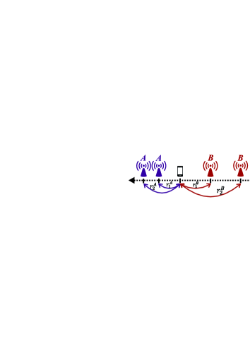
Figure 1: Motivational example with two technologies: $r_{1}^{A}<r_{1}^{B}$ and $r_{2}^{A}<r_{2}^{B}$.

Notably, the de facto standard association policy in existing wireless networks consists in associating each user equipment (UE) with the nearest base station (BS) or access point where one typical aim is to maximize the likelihood of being covered or connected. One of the main points of the present paper is that this is no longer optimal in these emerging virtual networks, as further discussed in Section I-A. The subtle distinction arising from technology diversity is illustrated in Fig. 1, where $r_{1}^{A}$ and $r_{2}^{A}$ (respectively, $r_{1}^{B}$ and $r_{2}^{B}$) denote the distances to the nearest and second-nearest BSs of technology $A$ (respectively, technology $B$) from the UE located at the origin. Also, we assume that $r_{1}^{A}<r_{1}^{B}$, i.e. the nearest BS of technology $A$ is the nearest to the UE, and there are only four BSs as shown in Fig. 1, which are identical except that they operate on different technologies (i.e. non-overlapping bandwidths). In the single technology case ($A=B$), the UE can simply associate with the BS at $r_{1}^{A}$. However, if $A\neq B$, e.g. the two technologies operate on different bandwidths, the locations of the strongest interferers, $r_{2}^{A}$ and $r_{2}^{B}$ (the second-nearest BSs), may overturn the choice of technology $A$ when the strongest interferer of technology $B$ is much farther from the UE than that of technology $A$, i.e. $r_{2}^{B}\gg r_{2}^{A}$, thus boosting the signal-to-noise-ratio (SINR) of technology $B$. In light of this example, optimal association in such networks requires sophisticated policies adaptively exploiting available information.

We can further generalize the above example and envisage a practical scenario where each UE can obtain the information about several received pilot signals of nearby BSs, as in 3G and 4G cellular networks, which can be translated into a vector of distances. In this paper, we are interested in investigating the following question.

Q: How much performance gain is achievable theoretically by tailoring the association policy and how much of it can we achieve in practice by exploiting available information?

Main Contributions: To tackle this association problem, we propose a stochastic geometry model of multi-technology wireless networks which partly builds upon [3]. This leads to a generic analytical framework lending itself to associating UEs to BSs in such a way that various performance metrics are optimized in the presence of the diversities alluded to above, and for various degrees of available information at the UE. In theoretical terms, the proposed framework paves the way for structural results on the partial ordering of optimal policy performance (see Section III) and a methodology for quantifying the performance of various association policies in a mathematically tractable manner. From the practical viewpoint, the results provide a mathematical edifice not only replacing exhaustive simulations but also usable for instance to analyze parsimonious association scheme, such as the max-ratio algorithm defined in the paper. We also prove asymptotic optimality of this pragmatic policy, which uses only the distances to the nearest and second-nearest BSs. Remarkably, all association schemes discussed in this work are underpinned by a user-centric approach leveraging the information about the network that is typically available at each UE in existing networks, thereby dispensing with any need for centralized coordination.

In the rest of the paper, after discussing the specificity of our problem with respect to previous work, we describe the notion of information exploited for the association in Sections II and III in order to characterize optimal association policies which in turn ameliorate performance indices, which are founded upon an underlying stochastic model of BSs and diverse types of information including fading values and distances to the BSs across different technologies. After establishing the optimality of the max-ratio algorithm under a limiting regime and deriving a versatile formula for computation of resulting performance in Sections IV and V, we derive tractable expressions for performance metrics of several association schemes and evaluate them in Sections VI and VII. The proofs of all the results are deferred to the Appendix.

I-A Related Work

The policy of associating each UE to the nearest BS or the BS with the strongest received power has been taken for granted in the vast literature on cell association. This is for instance the case in the stochastic geometry model of cellular networks [3]. The rationale is clear. This leads to the highest connectivity for each UE to choose the nearest BS unless it is possible to exploit the time-varying fading information, which is often unavailable in practice. Even with the recent emergence of heterogeneous wireless networks, also called HetNet, the rule is still valid in terms of coverage probability. That is, a UE is more likely to be covered if it associates with a BS whose received long-term transmission power (called pilot power) is the strongest. A stochastic geometry model to exploit this heterogeneous transmission powers of BSs belonging to multiple tiers in HetNets along with fading information has been investigated in [4].

However, from the perspective of load balancing between cells, the rule is invalid in general because each UE might be better off with a lightly-loaded cell rather than heavily-loaded one irrespective of the distances to them. In particular, in HetNet scenarios, it is important to distribute UEs to macro-cells and micro-cells so that they are equally loaded. The optimal association in the HetNet setting is inherently computationally infeasible, i.e. NP-Hard, whereas the potential gains from load-aware association schemes are much higher [5]. To tackle this problem, a few approximate or heuristic algorithms were proposed based on convex relaxations [5, 6] and non-cooperative and evolutionary games [7, 8]. Most of these algorithms are iterative in nature, requiring many rounds of messaging between UEs and BSs for their convergence.

It must be stressed that the multiple technology setting studied here is a largely unexplored territory where the validity of the standard rule to associate with the nearest BS is undermined, which is unprecedented in the literature as exemplified in Fig. 1. Lastly, while there have been considerable work adopting stochastic geometry models for analyzing given algorithms in large wireless networks, our work is a radical turnaround in the way of harnessing the model: we investigate new opportunities to tailor and design such algorithms to optimize the performance.

II Stochastic Network Model

In this paper, we consider adapting association schemes to ameliorate any performance metric in a downlink cellular network that is a function of the SINR received at a single typical UE. To this aim, we first describe a generic stochastic model of the network and define the general performance metric that is induced by an association policy of the UE of interest, which are assumed to be decoupled from those of other UEs. Note that we retain our stochastic network model in the most generic form for easier mathematical manoeuvrability of key results in Section III, which in fact holds for for a large class of point processes (PPs). For instance, the information structure $\mathcal{F}_{I}$ is simplified later in Section V.

II-A Network Model

We consider $T$ different technologies where $T$ is finite. The BS locations of technology $i\in[1,T]$ are assumed to be a realization of a homogeneous Poisson-Point Process (PPP) $\phi_{i}$ on $\mathbb{R}^{2}$ of intensity $\lambda_{i}$ independent of other PPPs. The typical user, from whose perspective we perform the analysis, is assumed to be located at the origin, without loss of generality. Denote by $r_{j}^{i}\in\mathbb{R}_{+}$ the distance to the $j$th closest point of $\phi_{i}$ to the origin, or equivalently the $j$th nearest BS, where ties are resolved arbitrarily. Hence $r^{i}_{1}$ denotes the distance to the closest point (BS) of $\phi_{i}$ from the origin.

Each BS of technology $i$ transmits at a fixed power $P_{i}$. The received power at a UE from any BS is however affected by fading effects and signal attenuation captured in the propagation model, typically through the path-loss exponent. We assume independent fading, i.e. the collection of fading coefficients $H_{j}^{i}$, which denotes the corresponding value from the $j$th nearest BS in technology $i$ to the UE, are jointly independent and identically distributed according to some distribution function. We model the propagation path loss through a non-increasing function $l_{i}(\cdot):\mathbb{R}_{+}\rightarrow\mathbb{R}_{+}$, where $i\in\{1,2,...,T\}$, i.e. the propagation model for each technology is determined by a possibly different attenuation function. Hence, the signal power received at the typical UE from the $j$th BS of technology $i$ is $P_{i}H^{i}_{j}l_{i}(r^{i}_{j})$. For mathematical brevity, we henceforth consider the point process $\phi_{i}$ of technology $i$ where each point is marked with an independent mark denoting the fading coefficient between the point (BS) to the origin (UE). We can assume that all the random variables belong to a single probability space denoted by $(\Omega,\mathcal{F},\mathbb{P})$ [9].

II-B Information at a UE

Another point at issue in this paper is the tradeoff between the cost of “information” available at UE and the performance gain attained by the association policy making use of that information. For easier presentation of results, e.g. Theorem III.1, the notion of information is encapsulated in a sigma-field $\mathcal{F}_{I}$ which is a sub-sigma algebra of the sigma-algebra $\mathcal{F}$ on which the marked point processes $\phi_{i}$ are defined. A sub-sigma algebra $\mathcal{F}^{{}^{\prime}}$ of $\mathcal{F}$ is such that $\mathcal{F}^{{}^{\prime}}\subseteq\mathcal{F}$. An example of information is $\mathcal{F}_{I}=\sigma\left(\cup_{i=1}^{T}\phi_{i}(B(0,w))\right)$, which corresponds to the sigma-field generated by the point process up to distance $w$ from the origin. In other words, the UE can estimate BS locations of different technologies $r_{j}^{i}$ such that $r_{j}^{i}\leq w$.

Notation	Brief Description
$\phi_{i}$	Point process corresponding to technology $i\in[1,T]$
$\lambda_{i}$	Intensity (density) of point process $\phi_{i}$
$p_{i}(\cdot)$	Performance function when associated with technology $i$
$\mathcal{F}_{I}$	Information available at the typical UE
$j_{i}$	$\arg\sup_{j\geq 1}\mathbb{E}[p_{i}(\text{SINR}_{0}^{i,j})|\mathcal{F}_{I}]$
$i^{*}$	The technology chosen by an association policy
$\mathcal{R}^{\pi}_{I}$	Average performance of association policy $\pi$ with $\mathcal{F}_{I}$
$\mathcal{R}^{\pi^{*}}_{I}$	Average performance of optimal policy $\pi^{*}$ with $\mathcal{F}_{I}$

TABLE I: Table of Notation

II-C Association Policies

An association policy governs the decisions on which technology and BS the typical user (who is located at the origin) should associate with. More formally, an association policy $\pi$ is a measurable mapping, i.e. $\pi:\Omega\rightarrow[1,T]\times\mathbb{N}$ which is $\mathcal{F}_{I}$ measurable. As stated before, we assume that all additional random variables needed by the policy $\pi$ are $\mathcal{F}_{I}$ measurable. The interpretation of the policy $\pi$ being $\mathcal{F}_{I}$ measurable is that a typical UE decides to choose a technology and a BS to associate with based only on the information obtainable in the network. It is important to note that while our discussion in this paper mainly revolves around optimal policies denoted by $\pi^{*}$, our methodology for the performance evaluation in Section V can be applied for any (suboptimal) policy.

II-D Performance Metrics

All performance metrics considered in this work are functions of SINR (Signal to Interference plus Noise Ratio) received at the typical UE. The SINR of the signal received at the origin from the $j$th nearest BS of technology $i$ is:

$$\text{SINR}_{0}^{i,j}=\frac{P_{i}H^{i}_{j}l_{i}(r^{i}_{j})}{N_{0}^{i}+\sum_{k\in\mathbb{N}\setminus\{j\}}P_{i}H^{i}_{k}l_{i}(r^{i}_{k})},$$

where $N_{0}^{i}$ is the thermal noise power which is a fixed constant for each technology $i\in\{1,2,...,T\}$. In order to encompass a general set of most useful performance metrics in wireless networks, the performance of different association policies are evaluated through non-decreasing functions of the SINR observed at the typical UE. Formally, let $p_{i}(\cdot):\mathbb{R}_{+}\rightarrow\mathbb{R}_{+}$ be a non-decreasing function for each $i\in\{1,2,...,T\}$ which represents the metric of interest if the typical UE associates with technology $i$. Since $\pi$ takes values in two coordinates $[1,T]\times\mathbb{N}$ (Section II-C), we divide them into separate coordinates which are denoted by $\pi(0)\in[1,T]$ and $\pi(1)\in\mathbb{N}$, respectively corresponding to the technology and BS chosen by the policy. Then the performance of the association policy $\pi$ when the information at the typical UE is quantified by $\mathcal{F}_{I}$ is then given by:

$$\mathcal{R}^{\pi}_{I}=\mathbb{E}[p_{\pi(0)}(\text{SINR}_{0}^{\pi})].$$ (1)

The subscript $I$ refers to the fact that the information present at the typical UE is $\mathcal{F}_{I}$. The performance metric $\mathcal{R}^{\pi}_{I}$ is averaged over all realizations of the BS deployments, fading variables, and any additional random variables used in the policy $\pi$.

Two well-known examples of performance metrics used in practice are coverage probability and average achievable rate. Coverage probability corresponds to setting the function $p_{i}(x)=\mathbf{1}(x\geq\beta_{i})$, which is the chance that the SINR observed at a UE from technology $i$ exceeds a threshold $\beta_{i}$. The other common performance metric of interest, average achievable rate, is defined as $p_{i}(x)=B_{i}\log_{2}(1+x)$, where the parameter $B_{i}$ is the bandwidth of technology $i$. All results on optimal association policy and performance evaluation are stated on the assumption of a general function $p_{i}(x)$.

III Optimal Association Policy

The optimal association policy denoted by $\pi^{*}$ is

$$\pi^{*}_{I}=\arg\sup_{\pi}\mathcal{R}^{\pi}_{I},$$ (2)

where the supremum is over all $\mathcal{F}_{I}$ measurable policies. From a practical point of view, the optimal association policy is the one that maximizes the performance of the typical UE among all policies having the same “information”. In this setup of optimal association, however, we always assume that the typical UE has knowledge of the densities $\lambda_{i}$ of the different technologies and the fact that they are independent PPPs although several fundamental results can be easily extended to more general point processes.

Since, we are interested in maximizing an increasing function of the SINR of the typical UE, the optimal association rule is clearly to pick the pair of technology and BS which yields the highest performance conditional on $\mathcal{F}_{I}$.

Proposition 1.

The optimal association algorithm when the information at the typical UE is given by the filtration $\mathcal{F}_{I}$ is such that

$$\begin{split}\pi^{*}_{I}(0)&=\arg\max_{i\in[1,T]}\sup_{j\geq 1}\mathbb{E}[p_{i}(\text{SINR}_{0}^{i,j})|\mathcal{F}_{I}],\\ \pi^{*}_{I}(1)&=\arg\sup_{j\geq 1}\max_{i\in[1,T]}\mathbb{E}[p_{i}(\text{SINR}_{0}^{i,j})|\mathcal{F}_{I}],\end{split}$$ (3)

where the UE must pick the technology $\pi^{*}_{I}(0)$ and the $\pi^{*}_{I}(1)$-th nearest BS to the origin in $\phi_{\pi^{*}_{I}(0)}$.

The performance of the optimal association is

$$\mathcal{R}^{\pi^{*}}_{I}=\mathbb{E}[\sup_{j\geq 1}\max_{i\in[1,T]}\mathbb{E}[p_{i}(\text{SINR}_{0}^{i,j})|\mathcal{F}_{I}]].$$ (4)

Since $[1,T]$ and $\mathbb{N}$ are countable sets, the order of the maxima in (4) does not matter. An important point to observe is that the optimal association given in (3) depends on the choice of the performance metric $\{p_{i}(\cdot)\}_{i=1}^{T}$. Hence, the optimal association rule would be potentially different if one was interested in maximizing coverage probability as opposed to maximizing rate-related metrics for instance.

III-A Ordering of the Performance of the Optimal Association

In this sub-section, we prove an intuitive theorem (Theorem III.1) stating that “more” information leads to better performance. To this aim, we need the following simple lemma.

Lemma 1.

Let $Y$ be any $\mathcal{E}$-valued R.V. and $g(\cdot):C\times\mathcal{E}\rightarrow\mathbb{R}$.

$$\mathbb{E}[\sup_{x\in C}g(x,Y)]\geq\sup_{x\in C}\mathbb{E}[g(x,Y)].$$

Theorem III.1.

If $\mathcal{F}_{I_{1}}\subseteq\mathcal{F}_{I_{2}}$, then $\mathcal{R}^{\pi^{*}}_{I_{1}}\leq\mathcal{R}^{\pi^{*}}_{I_{2}}$ where the association rule is the optimal one given in (3).

This theorem establishes a partial order on the performance of the optimal policy under different information scenarios at the UE for any performance functions $\{p_{i}(x)\}_{i=1}^{T}$.

III-B Optimal Association in the Absence of Fading Knowledge

The following lemma is quite intuitive and affirms that the optimal strategy for a UE in the absence of fading knowledge is to associate to the nearest BS of the optimal technology.

Lemma 2.

If the information $\mathcal{F}_{I}$ at the typical UE does not contain the fading random variables, then $j_{i}=\arg\sup_{j\geq 1}\mathbb{E}[p_{i}(\text{SINR}_{0}^{i,j})|\mathcal{F}_{I}]=1$ and hence $\pi^{*}_{I}(1)=j_{\pi^{*}_{I}(0)}=1$.

III-C Examples of Information

One common class of information is the “locally estimated information” which a UE may attain through measurements of (i) received long-term receive pilot signals, which can be easily converted into distances of BS, and (ii) instantaneous received signals, from which fading coefficients can be computed. For example, the knowledge of the distances to BSs no farther than $w$ from the UE is quantified through the sigma-algebra $\mathcal{F}_{w}=\sigma\left(\cup_{i=1}^{T}\mathcal{F}^{i}_{w}\right)$, where $\mathcal{F}^{i}_{w}=\sigma\left(\phi_{i}(B(0,w))\right)$ is the sigma algebra generated by the stochastic process $\phi(B(0,w))$. Furthermore, in case the UE is capable of estimating fading information, one can opt for the sigma-field generated by the marked stochastic process $\phi_{i}(B(0,w))$, denoted as $\mathcal{F}_{w}^{i,H}$, where each point (BS) is marked with a fading coefficient between the BS and the UE. Here the superscript $H$ refers to the sigma-field generated by the marked point-process.

In existing networks, the most practical example is the knowledge of the nearest $L$ BSs of each technology, denoted by $\mathbf{r}^{L}_{i}=[r^{1}_{i},..,r^{L}]$, i.e. the $L$-dimensional vector of the distances. In terms of sigma-algebra, it can be defined as $\mathcal{F}_{L}=\sigma\left(\cup_{i=1}^{T}\mathcal{F}^{i}_{L}\right)$, where $\mathcal{F}^{i}_{L}=\sigma\left(\phi_{i}(B(0,r^{L}_{i}))\right)$ is the knowledge of the $L$ nearest BS of each technology. One particularly intriguing scenario is complete information about the BS deployments, i.e. $L=\infty$. Denote by $\mathcal{F}_{\infty}$ the sigma-field for this information scenario and $\mathcal{R}^{\pi^{*}}_{\infty}$ as the performance obtained by the optimal policy knowing the entire network. Since $\mathcal{F}_{\infty}$ is the maximal element among all sub-sigma algebras of $\mathcal{F}$, it follows from Theorem III.1 that $\mathcal{R}^{\pi^{*}}_{\infty}$ is the the upper bound of all achievable performances. To strike a balance between the performance of interest and estimation cost at UE, each MVNO can evaluate $\mathcal{R}^{\pi^{*}}_{L}$ to see how much the association policy with $L$ distances stack up against the upper bound $\mathcal{R}^{\pi^{*}}_{\infty}$.

IV Max-Ratio Association Policy

While the parametric framework in Section III paves the way for designing the association policy maximizing various metrics, the optimal schemes encapsulated in (2) and (3) are amenable to tractable analysis only with the knowledge about the underlying PPPs $\phi_{i}$, i.e. their intensities $\lambda_{i}$. On the other hand, it is less conventional at the present time, if not unrealistic, to assume that the densities $\lambda_{i}$ are available at the UE in a real network. More importantly, in certain deployment scenarios, it is highly likely that the BS distribution follows a non-homogeneous point process with density (intensity) varying with the location over the network, thereby invalidating the homogeneous PPP assumption.

From the computational perspective, the optimal association can often demand substantial processing power of the UE particularly when the resulting association tailored for a specified performance metric is not simplified into a tractable closed-form expression. In this light, it is desirable to have policies that are completely oblivious to any statistical modeling assumption on the network, i.e. minimalistic policies exploiting universally available information such as distances to BSs, which can be computed from received pilot signal powers in 3G and 4G networks. To address these issues, we propose a max-ratio association policy. This policy has access to the ratio $r^{i}_{2}/r^{i}_{1}$ information for each technology $i$, i.e. the information $\mathcal{F}_{I}=\sigma\left(\cup_{i=1}^{T}r^{i}_{2}/r^{i}_{1}\right)$. The max-ratio association is formally described by

$$i^{*}=\max_{i\in[1,T]}r^{i}_{2}/r^{i}_{1},\text{ }j^{*}=1.$$

This ratio maximization implies that we place a high priority on a technology where simultaneously the distance to the nearest BS $r_{1}^{i}$ is smaller and that to the second-nearest BS $r_{2}^{i}$ is larger than other technologies. Note also that the above expression can be easily rearranged into the ratio of the received pilot powers of the nearest and second-nearest BSs when the BS transmission powers within each technology is the same. We show in Theorem IV.1 that although this policy per se is a suboptimal heuristic, it is optimal (in the sense of (3)) under a certain limiting regime of the wireless environment.

Theorem IV.1.

Let the noise powers $N^{i}_{0}=0$ for all technologies $i$ and the performance function for all technologies $p_{i}(\cdot)=p(\cdot)$ for all $i$. Consider the family of power-law path-loss functions $\{l^{(\alpha)}(\cdot)\}_{\alpha>2}$ where $l^{(\alpha)}(x)=x^{-\alpha}$. Let $k$ be any integer greater than or equal to $2$. If the information at the UE is the $k$-tuple of the nearest distances of each technology $i$ i.e. $\mathcal{F}_{I}=\sigma(\cup_{i=1}^{T}(r_{1}^{i}\cdots,r_{k}^{i}))$, then

$$\pi^{*}_{\alpha}(0)\xrightarrow[]{\alpha\rightarrow\infty}\operatornamewithlimits{arg\,max}_{i\in[1,T]}\frac{r_{2}^{i}}{r_{1}^{i}}\text{ a.s.},$$ (5)

where $\pi^{*}_{\alpha}$ is the optimal association as stated in (3). Recall $\pi^{*}_{\alpha}(1)=1$, $\forall\alpha$ from Lemma 2.

This theorem states that max-ratio association is optimal in cases where the signal is drastically attenuated (i.e. large path-loss exponents) with distance, e.g., metropolitan or indoor environments where the exponent reach values higher than 4, e.g. $\alpha\in[4,7]$. It is noteworthy that $\alpha$ at higher frequencies as in LTE networks tends to be higher (See, e.g. [10, Chapter 2.6] and references therein). In addition, another remarkable implication of this theorem is that it suffices for the asymptotic optimality to exploit the reduced information $r_{1}^{i}/r_{2}^{i}$ per technology in lieu of the given original information, i.e. $r_{1}^{i}$ and $r_{2}^{i}$. Also, any supplementary information on distances (or received pilot powers) to the third-nearest or farther BSs is superfluous and does not influence the optimality of the association. In Sections VI, we show that this association brings about surprisingly tractable expressions for key performance indices.

V Framework for Performance Analysis

In Section III, we compared the performance of the optimal association policy under different information scenarios by establishing a partial order on them without explicitly computing the performance $\mathcal{R}^{\pi}$. However, in order to quantify its impact on $\mathcal{R}^{\pi}$ without resorting to exhaustive simulations, one is also interested in its explicit expression for a given policy $\pi$, which may be an optimal policy as in Section III or a suboptimal one as in Section IV. We demonstrate how to explicitly compute $\mathcal{R}^{\pi}$ in an automatic fashion (in Theorem V.1) for any arbitrary policy $\pi$ belonging to a large class of polices, called generalized association, which constitutes another part of our contribution.

V-A Generalized Association

In the rest of the paper, we restrict our discussion to a class of association policies $\pi$ that are optimized over information with a special structure $\mathcal{F}_{I}$, incorporating what is conventionally available in cellular networks. That is, in order to answer the question posed in I, we assume that the form of information that a UE has about each technology $i$ is a vector $\mathbf{r}_{i}\in\mathbb{R}^{L}$. For instance, if the mobile is informed of the smallest two distances of each technology and their instantaneous signal powers, then $\mathbf{r}_{i}$ is a 4-dimensional vector with $2$ dimensions representing the distances and the other $2$ dimensions corresponding to the instantaneous fading powers. That is, we adopt this reduced notation as a surrogate for the sigma-algebra notation in Section III for simplicity of the exposition. Formally, we assume that the association policy $\pi=\{\pi_{i}(\cdot)\}_{i=1}^{T}$, according to which a mobile chooses a technology to associate with is given by

$$i^{*}=\arg\max_{i\in[1,T]}\pi_{i}(\mathbf{r}_{i},\lambda_{i}),$$ (6)

where $j_{i}$, the index of BS of technology $i$ to which the UE associates conditioned on selection of $i$, i.e. $i=i^{*}$, and $\mathbf{r}_{i}$ is the $L$-dimensional vector of observation for technology $i$.

It is noteworthy that when the technologies are operated on overlapping bandwidths, the above form of association may be extended to a more general form $\pi_{i}(\{\mathbf{r}_{i}\}_{i=1}^{T},\{\lambda_{i}\}_{i=1}^{T})$, where each association policy utilizes not only the information regarding technology $i$ but also that about all other technologies. Envisioning this extension is easily justifiable because the desirability of technology $i$ (represented by $\pi_{i}(\cdot)$) is affected by the interference inflicted by other technologies. However, we leave it as future work and focus our discuss onto the restricted class of information $\mathcal{F}_{I}$ in (6) which covers most interesting scenarios in case of non-overlapping frequency bandwidths.

V-B Performance Computation of the Generalized Association

For each technology $i$, we denote by $f_{i}(\mathbf{r}_{i})$ the probability density function (pdf) of the information vector $\mathbf{r}_{i}$ of technology $i$. For instance, if $L=1$ and each mobile has knowledge about the location of the nearest base-station $r_{1}^{i}$, then it follows from the property of a PPP that $f_{i}(\mathbf{r}_{i})=f_{i}(r_{1}^{i})$ is the Rayleigh distribution with parameter $1/\sqrt{2\pi\lambda_{i}}$. As for the max-ratio policy, $f_{i}(\mathbf{r}_{i})=f_{i}([r_{1}^{i},r_{2}^{i}])$ becomes the distribution of the nearest and second-nearest BSs characterized by the underlying PPP of technology $i$. We also denote by $f_{i}^{*}(\mathbf{r})$ the pdf of the vector $\mathbf{r}_{i}$ conditioned on the event that technology $i$ is selected, i.e. $i^{*}=i$.

Denote by $f_{\pi_{i}}(\cdot)$ the pdf of $\pi_{i}(\mathbf{r}_{i},\lambda_{i})$ and by $F_{\pi_{i}}(\cdot)$ the cumulative density function (cdf) of $\pi_{i}(\mathbf{r}_{i},\lambda_{i})$. To put it simply, $f_{\pi_{i}}(\cdot)$ is the cdf of a function $\pi_{i}(\cdot)$ of the given information $\mathbf{r}_{i}$ rather than that of $\mathbf{r}_{i}$ itself. For example, in case of the max-ratio policy, $f_{\pi_{i}}(\cdot)$ is the distribution of $r_{2}^{i}/r_{1}^{i}$. To prove the main theorem, we first need to delineate the interplay between the distribution of optimal technology $f_{i}^{*}(\cdot)$, its original distribution $f_{i}(\cdot)$, and the (cumulative) distribution of the association policy $F_{\pi_{i}}(\cdot)$. We have the following lemma from a direct application of Bayes’ rule and independence of the point processes $\phi_{i}$.

Lemma 3.

The probability density function $f_{i}^{*}(\mathbf{r})$ is given by

$$f^{*}_{i}(\mathbf{r})=f_{i}(\mathbf{r})\cdot\frac{1}{\mathbb{P}[i^{*}=i]}\cdot\prod_{j=1,j\neq i}^{T}F_{\pi_{j}}(\pi_{i}(\mathbf{r},\lambda_{i})).$$ (7)

The following theorem finally presents a direct method for computing the performance of any generalized association policy $\pi$. Recall that the performance of a policy $\pi$ is given by $\mathcal{R}^{\pi}_{I}=\mathbb{E}[p_{i^{*}}(\text{SINR}_{0}^{i^{*},j_{i^{*}}})]$.

Theorem V.1.

The performance of the association algorithm $\pi$ under information $\mathcal{F}_{I}$ denoted by $\mathcal{R}^{\pi}_{I}$ is given by-

$$\sum_{i=1}^{T}\int_{\mathbf{r}\in\mathbb{R}^{L}}\mathbb{E}[p_{i}(\text{SINR}_{0}^{i,j_{i}})|\mathbf{r}]f_{i}(\mathbf{r})\prod_{j=1,j\neq i}^{T}F_{\pi_{j}}(\pi_{i}(\mathbf{r},\lambda_{i}))d\mathbf{r},$$ (8)

where $\mathbb{E}[p_{i}(\text{SINR}_{0}^{i,j_{i}})|\mathbf{r}]$ corresponds to the performance obtained by associating to technology $i$ conditioned on the information about technology $i$ the UE has is the vector $\mathbf{r}$.

This theorem states that we need only two expressions, information distribution $f_{i}(\cdot)$ and policy distribution $f_{\pi_{i}}(\cdot)$, in order to derive the performance metric. As exemplified earlier, while $f_{i}(\cdot)$ is usually a simplistic expression thanks to properties of PPP, mathematical manipulability of $f_{\pi_{i}}(\cdot)$ highly relies on the complexity of the association policy.

VI Computational Examples

In this section, we leverage the results in Section V to derive several performance metrics in selected practical scenarios where the association policy utilizes information $\mathcal{F}_{I}$ restricted to a vector of distances to BSs ($\mathbf{r}_{i}$) and BS densities ($\lambda_{i}$) as shown in (6). Note however that one can directly compute the performance ($\mathcal{R}^{\pi}_{I}$ in Theorem V.1) with the probability density function of any association policy ($f_{i}(\mathbf{r})$) by exploiting Lemma 7. We show that the resulting performance expressions are mathematically tractable and lend themselves to quantifying the performance of large-scale wireless networks.

For the rest of this section, we consider two representative metrics: (i) coverage probability $p_{i}(x)=\mathbf{1}(x\geq\beta_{i})$ and (ii) average achievable rate where, to simplify the exposition, we assume the bandwidths of different technologies are the same, i.e. $p_{i}(x)=p(x)=\log_{2}(1+x)$. However, Theorem V.1 can be used to compute the performance of any arbitrary non-decreasing function $p_{i}(\cdot)$. We also assume that the fading variable $H_{j}^{i}$ is exponential, i.e. Rayleigh fading, with mean $\mu^{-1}$ and the path-loss function $l_{i}(r)=r^{-\alpha}$ for $\alpha>2$ for all $i\in[1,T]$. These assumptions have often been adopted for analysis of wireless systems [10] and espoused in stochastic geometry models [9, 11].

Let us denote by $c_{p}(j;\mathbf{r},\lambda,P,\beta)$ the coverage probability of a UE at the origin served by the $j$th nearest BS to the origin where the BSs are spatially distributed as a PPP of intensity $\lambda$. Here each BS transmits at power $P$ and we are interested in the probabilistic event that the received SINR exceeds the threshold $\beta$. The vector $\mathbf{r}$ denotes the vector of distances to BSs, based on which the association decision will be made. More formally,

$$c_{p}(j;\mathbf{r},\lambda,P,N_{0},\beta)=\mathbb{E}\left[\mathbf{1}\left(\frac{PH_{j}}{N_{0}+\sum_{k\neq j}PH_{k}}\geq\beta\right)\bigg{|}\mathbf{r}\right.]$$ (9)

Likewise, we denote by $r(j;\mathbf{r},\lambda,P)$ the expected rate received by a typical UE at the origin when it is being served by the $j$th nearest BS to the origin where the BSs are distributed as a PPP of intensity $\lambda$ and transmitting at power level $P$:

$$r(j;\mathbf{r},\lambda,P,N_{0}) =\mathbb{E}\left[\log_{2}\left(1+\frac{PH_{j}}{N_{0}+\sum_{k\neq j}PH_{k}}\right)\bigg{|}\mathbf{r}\right]$$

$$=\int_{t\geq 0}c_{p}(j;\mathbf{r},\lambda,P,N_{0},2^{t}-1)dt.$$ (10)

Therefore, once we derive an expression for the coverage probability, the average achievable rate expression follows immediately from the calculation of the simple integral in (10). In the sequel, we first compute technology-wise expressions, (9) and (10), which are in turn plugged as $p_{i}(\cdot)$ into Theorem V.1 to yield coverage probability metric $\mathcal{R}^{cp}$ and average achievable rate metric $\mathcal{R}^{r}$, respectively.

VI-A Optimal Association Policy

Recall that in the absence of knowledge of fading information, the optimal association policy is to choose technology $i^{*}$ such that:

$$i^{*} =\arg\max_{i\in[1,T]}c_{p}(1;r_{i},\lambda_{i},P_{i},N_{0}^{i},\beta_{i}),$$ (11)

$$i^{*} =\arg\max_{i\in[1,T]}r(1;r_{i},\lambda_{i},N_{0}^{i},P_{i}),$$ (12)

respectively for coverage probability and average achievable rate. Note also that it follows from Lemma 2 that it is unconditionally optimal to choose the nearest BS for each technology, i.e. $j^{*}=1$. Thus our discussion in this section is focused on the choice of technology $i$.

In this example, we investigate two cases where the UE has knowledge of the distances to the nearest $r_{1}^{i}$ or up to the second-nearest BSs $[r_{1}^{i},r_{2}^{i}]$ along with the densities of technologies $\lambda_{i}$ while being oblivious to the information about fading $H_{j}^{i}$. In comparison with the standard rule to associate with the nearest BS, this example demonstrates how our proposed framework can be used not only to design an optimal association algorithm maximizing a performance index but also to compute the resulting performance improvements arising from the additional knowledge of distances and densities. The following theorem delineates, among all technologies $i\in[1,T]$, which technology yields the best coverage probability metric.

Theorem VI.1.

If the UE has the knowledge about $r_{1}^{i}$, for all $i\in[1,T]$, the association rule (11) with the following expression maximizes the coverage probability:

$$c_{p}(1;r_{1},\lambda,P,N_{0},\beta)={\rm e}^{-\mu\beta N_{0}r_{1}^{\alpha}P^{-1}}\\ \exp\left(-2\pi\lambda\int_{u=r_{1}}^{\infty}\frac{1}{1+\beta^{-1}\left(u/r_{1}\right)^{\alpha}}udu\right).$$ (13)

If the UE has the knowledge about $r_{1}^{i}$ and $r_{2}^{i}$, for all $i\in[1,T]$, the association rule (11) with the following expression maximizes the coverage probability:

$$c_{p}\left(1;[r_{1},r_{2}],\lambda,P,N_{0},\beta\right)={\rm e}^{-\mu\beta N_{0}r^{\alpha}_{1}P^{-1}}\frac{1}{1+\beta\left(r_{1}/r_{2}\right)^{\alpha}}\\ \exp\left(-2\pi\lambda\int_{u=r_{2}}^{\infty}\frac{1}{1+\beta^{-1}\left(u/r_{1}\right)^{\alpha}}udu\right).$$ (14)

To better understand the practical implications of (13), we can consider the case where the thermal noise and threshold terms are identical, i.e. $N_{0}^{i}=N_{0}$ and $\beta_{i}=\beta$. Since both the first and second factors in the right-hand side of (13) are decreasing functions with respect to $r_{1}$, the above policy gives preference to smaller $r_{1}^{i}$ among all technologies $i\in[1,T]$, which is in line with our intuition.

However, for approximately similar values of $r_{1}^{i}$, it also reveals that the optimal policy tends to choose technology $i$ with lower density $\lambda_{i}$ because the right-hand side of (13) decreases with $\lambda$. The observation is in best agreement with our intuition again because technology $i$ with high density $\lambda_{i}$ implies that there are more interfering BSs on the average. On the other hand, the standard rule leads to higher chance of association with the technology with large $\lambda_{i}$ because the nearest BS is more likely to belong to the technologies consisting of higher number of BSs. Thus it can be deduced that in case of heterogeneous BS densities, the standard rule leads to very poor coverage performance because of its tendency to associate with the most populous technology, whereas the above equation reveals the optimality of associating with sparsely populated technology, which sheds light on the complex optimization to be carried out by MVNOs. Likewise, the optimal policy exploiting the additional information of $r_{2}^{i}$ exhibits similar tendencies in (14) while it prefers technology $i$ with larger $r_{2}^{i}$, thus pushing the strongest interference signal as far as possible.

In order to compute the optimal performance metric $\mathcal{R}^{cp}$ resulting from the association rule maximizing the coverage probability, we first need to derive the probability distribution of $c_{p}(1;r,\lambda_{i},P_{i},N_{0},\beta)$, which is in turn plugged into Theorem V.1. The CDF $F_{\pi_{i}}(y)=\mathbb{P}[c_{p}(1;r,\lambda_{i},P_{i},N_{0},\beta)\leq y]$ can be simplified into the following expression by using the fact that the nearest distance $r$ of BSs distributed as a PPP is Rayleigh distributed with parameter $\frac{1}{\sqrt{2\pi\lambda_{i}}}$.

Lemma 4.

The CDF $F_{\pi_{i}}(\cdot)$ is given by

$$F_{\pi_{i}}(y)=e^{-\ln\left(\frac{1}{y}\right)\frac{1}{2}\left(\int_{v=1}^{\infty}\frac{1}{1+\beta^{-1}\left(v\right)^{\alpha}}vdv\right)^{-1}}.$$ (15)

Finally, plugging (15) into (8), we get the following theorem on the coverage probability maximized by the optimal association policy.

Corollary 1.

The coverage probability resulting from the optimal association exploiting the knowledge of $r_{1}^{i}$ is

$$\mathcal{R}^{cp}=\sum_{i=1}^{T}\int_{\mathbf{r}\in\mathbf{R}}c_{p}(1;r,\lambda_{i},P_{i},N_{0}^{i},\beta_{i})2\pi\lambda_{i}re^{-\pi\lambda_{i}r^{2}}\\ \prod_{j=1,j\neq i}^{T}\left(\frac{1}{c_{p}(1;r,\lambda_{j},P_{j},N_{0}^{j},\beta_{j})}\right)^{-\frac{1}{2}\left(\int_{v=1}^{\infty}\frac{1}{1+(\beta_{j})^{-1}\left(v\right)^{\alpha}}vdv\right)^{-1}}.$$ (16)

VI-B Max-Ratio Association Policy

Recall that in the absence of fading information, the Max-Ratio algorithm described in Section IV is to choose technology such that $i^{*}=\max_{i\in[1,T]}{r^{i}_{2}}/{r^{i}_{1}}$ with the nearest BS in the chosen technology, i.e. $j^{*}=1$. Although we saw in Section VI-A that the density information play a crucial role in performing optimal association, we know from Theorem IV.1 that the simple non-parametric policy of Max-Ratio is optimal in the limit of large path-loss. In this section, we also show that this policy is tractable and yields expressions for key performance metrics (Corollary 19 and 20). The simplistic form of the policy distribution $F_{\pi_{i}}(\cdot)$ in the following lemma alludes to ensuing tractable results in this section.

Lemma 5.

The law $F_{\pi_{i}}(\cdot)$ for the max-ratio algorithm is:

$$F_{\pi_{i}}(x)=\mathbb{P}\left[r^{i}_{2}/r^{i}_{1}\leq x\right]=1-1/x^{2}.$$ (17)

Corollary 2.

The coverage probability performance $\mathcal{R}^{cp}$ of the max-ratio algorithm is given by

$$2\sum_{i=1}^{T}\int_{t\geq 1}c_{p}\left(1;\frac{r^{i}_{2}}{r^{i}_{1}}=t,\lambda_{i},P_{i},N_{0}^{i},\beta_{i}\right)\frac{1}{t^{3}}\left(1-\frac{1}{t^{2}}\right)^{T-1}dt,$$ (18)

where

$$c_{p}\left(1;\frac{r^{i}_{2}}{r^{i}_{1}}=t,\lambda_{i},P_{i},N_{0}^{i},\beta_{i}\right)=\\ \int_{u=0}^{\infty}c_{p}\left(1;\left[u,ut\right],\lambda_{i},P_{i},N_{0}^{i},\beta_{i}\right)2(\pi\lambda_{i})^{2}u^{3}t^{4}e^{-\lambda\pi(ut)^{2}}du,$$ (19)

where $c_{p}\left(1;\left[u,ut\right],\lambda_{i},P_{i},N_{0}^{i},\beta_{i}\right)$ is given in (14).

Since the max-ratio does not optimize a particular performance metric but merely compares the ratio $r_{2}^{i}/r_{1}^{i}$, the average achievable rate expression can be obtained directly from the integral transform in (10), which in turn is plugged into Theorem IV.1 to yield the following corollary.

Corollary 3.

The average achievable rate of the max-ratio algorithm is

$$\mathcal{R}^{r}=2\sum_{i=1}^{T}\int_{v\geq 0}\int_{t\geq 1}c_{p}\left(1;\frac{r^{i}_{2}}{r^{i}_{1}}=t,\lambda_{i},P_{i},2^{v}-1\right)\\ \frac{1}{t^{3}}\left(1-\frac{1}{t^{2}}\right)^{T-1}dtdv,$$ (20)

where $c_{p}\left(1;\frac{r^{i}_{2}}{r^{i}_{1}}=t,\lambda_{i},P_{i},2^{v}-1\right)$ is given in (19).

To get more intuition about the formula, we present the following corollary.

Theorem VI.2.

In the Interference-limited regime (i.e. $N_{0}^{i}=0$ for all $i\in[1,T]$), if the path-loss function is given by $l_{i}(r)=r^{-\alpha}$ for some $\alpha>2$ and all $i\in[1,T]$, the coverage probability and the average achievable rate of the max-ratio algorithm are respectively given by

$$\textstyle\mathcal{R}^{cp}=\left\{\begin{array}[]{ll}\displaystyle\sum_{i=1}^{T}\int_{x=0}^{1}\textstyle\frac{2(T-1)\cdot x^{3}(1-x^{2})^{T-2}}{1+\beta_{i}^{2/\alpha}\phi(\alpha,\beta_{i},x)}dx,&T\geq 2\\ \frac{1}{1+\beta_{1}^{2/\alpha}\phi(\alpha,\beta_{1},1)},&T=1\end{array}\right.,$$ (21)

$$\textstyle\mathcal{R}^{r}=\left\{\begin{array}[]{ll}\displaystyle\sum_{i=1}^{T}\int_{x=0}^{1}\int_{t\geq 0}\textstyle\frac{2(T-1)\cdot x^{3}(1-x^{2})^{T-2}}{1+(2^{t}-1)^{2/\alpha}\phi(\alpha,2^{t}-1,x)}dtdx,&T\geq 2\\ \displaystyle\int_{t\geq 0}\textstyle\frac{1}{1+(2^{t}-1)^{2/\alpha}\phi(\alpha,2^{t}-1,1)}dt,&T=1,\end{array}\right.$$ (22)

where the function $\phi$ is given by

$$\phi(\alpha,y,x)=\int_{u\geq y^{-2/\alpha}}\frac{1}{1+x^{-\alpha}u^{\alpha/2}}du.$$

Since the case $T=1$ in the above theorem corresponds to the standard rule to associate with the nearest BS in the presence of only one technology, Equations (21) and (22) reduce to much simpler expressions compared to those in the literature, e.g. Sections III-D and IV-C in the work [3]. On the other hand, as $T$ becomes larger, inside integrand in (21), the distribution $2T(T-1)x^{3}(1-x^{2})^{T-2}$ (additional $T$ cancels out the summation operation) is gradually skewed toward the origin $x=0$, around which $\phi(\alpha,\beta_{i},x)$ approaches 0. It is easy to show that the coverage probability $\mathcal{R}^{cp}$ approaches one with higher technology diversity, i.e. $T\to\infty$. Though it is not realistic to envision such a large number of technologies or operators, from which each UE can cherry-pick its optimal BS, this theorem demonstrates how much UEs potentially benefit from the multiple bandwidths or technologies pooled by MVNOs.

Contrary to the standard association which tends to pick more populous technologies (i.e. large $\lambda_{i}$), giving rise to higher number of interferers, the max-ratio policy counterbalances this pathological behavior by ensuring that the strongest interferer $r_{2}^{i}$ is located relatively further. At the same time, the overall performance of max-ratio algorithm critically relies on large path-loss constant $\alpha$, whereas with this caveat, Theorem IV.1 states that the algorithm is asymptotically optimal as $\alpha\to\infty$ for any increasing performance function $p_{i}(\cdot)=p(\cdot)$ in the interference-limited regime.

VII Simulations and Numerical Results

In this section, we provide more insights into our framework and results by performing simulations and noticing their trends. In performing the simulations, we take as performance metrics, the coverage probability with $p_{i}(x)=\mathbf{1}(x\geq\beta_{i})$ and the average rate with $p_{i}(x)=\log_{2}(1+x)$.

VII-A Diminishing Returns with Increasing Information

We first observe through simulations that the optimal association for any good class of performance metrics (made precise in the sequel) exhibits the law of diminishing returns. The term, diminishing returns, is used in the context where the additional gains or improvements in performance of optimal association reduces as the information increases. Fig. 2 shows that coverage probability with the optimal association exploiting the knowledge of the nearest $k$ BS of each technology. As we move on the x-axis, we are increasing the information known at the UE and observe that the gains saturate drastically. Remarkably, beyond learning the $2$ nearest BSs per technology, there is no tangible improvement in the coverage probability. This implies that in practice, it is sufficient for each UE to learn the nearest two BSs per technology which will yield almost all the optimal performance possible with the full information about the topology.

We present a simple argument why one would expect to see diminishing returns for any performance metric. Assume we have some “good” performance metric functions $\{p_{i}(\cdot)\}_{i=1}^{T}$, i.e. $\mathbb{E}[p_{i}(\text{SINR}^{i,j}_{0})]$ is upper-bounded for all $i\in[1,T]$ and all $j\in\mathbb{N}$. Let $\{\mathcal{F}_{n}\}_{n\in\mathbb{N}}$ be a filtration of information $\mathcal{F}$ such that i.e. $\mathcal{F}_{n}\subseteq\mathcal{F}_{n+1}\subseteq\mathcal{F}$ for all $n$. Denote by $\mathcal{F}_{\infty}$ as the limit of $\mathcal{F}_{n}$, i.e. $\mathcal{F}_{\infty}=\cup_{n\geq 1}\mathcal{F}_{n}$ and let $\mathcal{R}^{\pi^{*}}_{n}=\mathbb{E}[\sup_{j\geq 1}\max_{i\in[1,T]}\mathbb{E}[p_{i}(\text{SINR}^{i,j}_{0})||\mathcal{F}_{n}]]$ be the performance of the optimal association policy under information $\mathcal{F}_{n}$. Theorem III.1 then gives that the sequence $\{\mathcal{R}^{\pi^{*}}_{n}\}_{n\geq 1}$ is non-decreasing and $\mathcal{R}^{\pi^{*}}_{\infty}<\infty$. Any such sequence of bounded and non-decreasing numbers contains a sub-sequence $\{\mathcal{R}^{\pi^{*}}_{n_{i}}\}_{i}$ such that the gains $\Delta_{n_{i}}=R^{\pi^{*}}_{{n}_{i+1}}-R^{\pi^{*}}_{n_{i}}$ decreases with $i$. Therefore, the law of diminishing returns property holds.

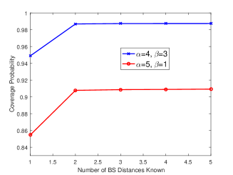
Figure 2: The diminishing returns with increasing information with $T=10$, the path-loss function $l_{i}(r)=r^{-\alpha}$, and the performance $p_{i}(x)=\mathbf{1}(x\geq\beta)$.

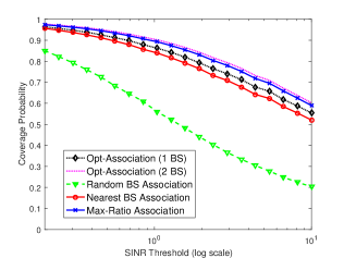
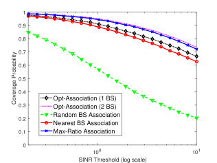
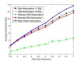
Figure 3: Comparison of various association schemes. The first two graphs on the left compare coverage probability where $l_{i}(r)=r^{-4}$ and $T=5$ for the first figure and $T=8$ for the second figure. The rightmost graph compares average achievable rate where $\alpha$ is varied on the x-axis and $l_{i}(r)=r^{-\alpha}$.

VII-B Comparison of Schemes and Technology Diversity

The first two graphs in Fig. 3 compare the coverage probability of various association schemes with path-loss exponent $\alpha=4$ for different number of technologies, $T=5$ and $T=8$. We observe in all graphs that the Max-Ratio association scheme outperforms the optimal association policy under the case when only the nearest BS distances are known. More importantly, the Max-ratio association performs almost as well as the optimal association under the knowledge of nearest $2$ BSs per technology for this typical value of path-loss exponent, not to mention that it outperforms the nearest BS association significantly, particularly when the technology diversity is higher, i.e. $T=8$.

The rightmost graph in Fig. 3 depicts the average achievable rate for path-loss exponents $\alpha\in[2.5,7]$, which empirically corroborates the statement of Theorem IV.1 that Max-Ratio is the optimal policy when nearest $k\geq 2$ BS per technology are known in the high path-loss regime. Remarkably, Max-Ratio and the optimal association with two nearest BS distances performs almost equally (indistinguishable in the graph) for $\alpha\geq 5$. That is, a simple non-parametric policy like the max-ratio performs as well as the optimal association policy in which the entire network topology is known (the best possible performance) even in the finite path-loss case. It is also noted that the random BS association, which is the only policy oblivious to technology diversity, results in poor performance in all cases. Thus it is beneficial for MVNOs to leverage the technology diversity in any possible manner by all means.

As shown in Fig. 4, the coverage probability tends to one as $T$ goes to infinity, as discussed in Section VI-B. The performance of Max-Ratio algorithm however reaches one quicker than nearest BS association. This shows that Max-Ratio exploits this diversity better than the conventional scheme to associate to the nearest BS.

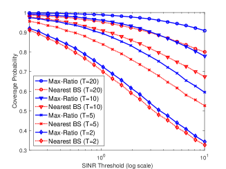
Figure 4: Coverage probability increases with technology diversity $T$.

VIII Conclusions

In this work, we explored the potential to boost the service performance of wireless networks without incurring additional infrastructure cost by capitalizing on a new form of diversity, which can be either several networks operated on orthogonal bandwidths or multiple wireless technologies pooled by some mobile virtual network operators. We proposed a generic stochastic geometry model for designing association policies proactively optimizing desired performance metrics. We also showed that the most important metrics can in turn be evaluated via a generic formula. Combined with another result characterizing the gradual increase of performance with respect to the amount of information, the framework provides a theoretical upper bound on the given metric, which can be used to determine the balance between the cost of estimating information at a mobile and the performance gain. Lastly, we devised a pragmatic association scheme exploiting only two received pilot powers, whose asymptotic optimality is established under a limiting regime of high path-loss. As shown in the simulations, this scheme can serve as an alternative to the standard rules in urban or metropolitan environments with severe signal attenuation which better exploits the new form of diversity.

IX Acknowledgements

This work was supported by an award from the Simons Foundation (# 197982) to The University of Texas at Austin.

-A Proof of Lemma 1

Proof:

We have

$$\sup_{x\in C}g(x,Y) \geq g(x,Y)\text{ }\forall x\in C,$$

and hence

$$\mathbb{E}[\sup_{x\in C}g(x,Y)]\geq\mathbb{E}[g(x,Y)]\text{ }\forall x\in C.$$ (23)

Since (23) is valid for all $x\in C$, we can pick the supremum on the RHS, i.e.

$$\mathbb{E}[\sup_{x\in C}g(x,Y)]\geq\sup_{x\in C}\mathbb{E}[g(x,Y)].$$ (24)

-B Proof of Theorem III.1

Proof:

$$\mathcal{R}^{\pi^{*}}_{I_{2}} =\mathbb{E}[\max_{i\in[1,T]}\sup_{j\geq 1}\mathbb{E}[p_{i}(\text{SINR}_{0}^{i,j})|\mathcal{F}_{I_{2}}]]$$

$$\stackrel{{\scriptstyle(a)}}{{=}}\mathbb{E}[\mathbb{E}[\max_{i\in[1,T]}\sup_{j\geq 1}\mathbb{E}[p_{i}(\text{SINR}_{0}^{i,j})|\mathcal{F}_{I_{2}}]|\mathcal{F}_{I_{1}}]]$$

$$\stackrel{{\scriptstyle(b)}}{{\geq}}\mathbb{E}[\max_{i\in[1,T]}\sup_{j\geq 1}\mathbb{E}[\mathbb{E}[p_{i}(\text{SINR}_{0}^{i,j})|\mathcal{F}_{I_{2}}]|\mathcal{F}_{I_{1}}]]$$

$$\stackrel{{\scriptstyle(c)}}{{=}}\mathbb{E}[\max_{i\in[1,T]}\sup_{j\geq 1}\mathbb{E}[p_{i}(\text{SINR}_{0}^{i,j})|\mathcal{F}_{I_{1}}]]=\mathcal{R}^{\pi^{*}}_{I_{1}}$$

where $(a)$ follows from the tower property of expectation, $(b)$ follows from Lemma 1 and $(c)$ follows from the tower property of expectation and the fact that $\mathcal{F}_{I_{1}}\subseteq\mathcal{F}_{I_{2}}$.

-C Proof of Lemma 2

Proof:

From the properties of PPP, we know that almost-surely, the distances $\{r^{i}_{k}\}_{k\geq 1}$ are distinct i.e. satisfy $r^{i}_{k}>r^{i}_{k+1}$. Denoting $S_{k}=P_{i}l_{i}(r^{i}_{k})$ for each $k\in\mathbb{N}$ (instead of representing it as $S^{i}_{k}$, we drop the $i$ in this proof for simplicity), we can write (3) as

$$j_{i} =\arg\sup_{j\geq 1}\mathbb{E}\left[p_{i}\left(\frac{S_{j}H_{j}}{N_{0}^{i}+\sum_{d\neq j}S_{d}H_{d}}\right)\bigg{|}\mathcal{F}_{I}\right]$$

$$\stackrel{{\scriptstyle(a)}}{{=}}\arg\sup_{j\geq 1}\mathbb{E}\left[\frac{S_{j}H_{j}}{N_{0}^{i}+\sum_{i\neq j}S_{i}H_{i}}\bigg{|}\mathcal{F}_{I}\right],$$

where $(a)$ follows from the fact that the function $p_{i}(\cdot)$ is non-decreasing.

$$\sup_{j\geq 1}\mathbb{E}\left[\frac{S_{j}H_{j}}{N_{0}^{i}+\sum_{d\neq j}S_{d}H_{d}}\bigg{|}\mathcal{F}_{I}\right]$$

$$=\sup_{j\geq 1}\mathbb{E}\left[\mathbb{E}\left[\frac{S_{j}H_{j}}{N_{0}^{i}+\sum_{d\neq j}S_{d}H_{d}}\bigg{|}\sigma(\mathcal{F}_{I}\cup\phi_{i})\right]\bigg{|}\mathcal{F}_{I}\right]$$

$$\leq\mathbb{E}\left[\sup_{j\geq 1}\mathbb{E}\left[\frac{S_{j}H_{j}}{N_{0}^{i}+\sum_{d\neq j}S_{d}H_{d}}\bigg{|}\sigma(\mathcal{F}_{I}\cup\phi_{i})\right]\bigg{|}\mathcal{F}_{I}\right],$$ (26)

where the inequality follows from Lemma 1. Since conditioned on $\phi_{i}$, we have $S_{k}$ deterministic and $H_{k}$ conditionally i.i.d. given $\phi_{i}$ and independent of $\mathcal{F}_{I}$, we have

$$\sup_{j\geq 1}\mathbb{E}\left[\frac{S_{j}H_{j}}{N_{0}^{i}+\sum_{d\neq j}S_{d}H_{d}}\bigg{|}\sigma(\mathcal{F}_{I}\cup\phi_{i})\right]$$

$$=\sup_{j\geq 1}\mathbb{E}\left[{S_{j}H_{j}}|\sigma(\mathcal{F}_{I}\cup\phi_{i})\right]\mathbb{E}\left[\frac{1}{N_{0}^{i}+\sum_{d\neq j}S_{d}H_{d}}\bigg{|}\sigma(\mathcal{F}_{I}\cup\phi_{i})\right]$$

$$=\sup_{j\geq 1}\mathbb{E}\left[{S_{j}H_{j}}|\phi_{i}\right]\mathbb{E}\left[\frac{1}{N_{0}^{i}+\sum_{d\neq j}S_{d}H_{d}}\bigg{|}\phi_{i}\right].$$ (27)

Thus $j=1$ achieves the supremum in (27) since $S_{k}>S_{k+1}$ and is deterministic given $\phi_{i}$. Combining this fact with (26), we have

$$\sup_{j\geq 1}\mathbb{E}\left[\frac{S_{j}H_{j}}{N_{0}^{i}+\sum_{d\neq j}S_{d}H_{d}}\bigg{|}\mathcal{F}_{I}\right]\leq\mathbb{E}\left[\frac{S_{1}H_{1}}{N_{0}^{i}+\sum_{d\geq 2}S_{d}H_{d}}\bigg{|}\mathcal{F}_{I}\right],$$ (28)

which yields that $j_{i}=1$.

-D Proof of Theorem IV.1

Proof:

For ease of notation, we denote the path-loss function as simply $l(\cdot)$ instead of $l^{(\alpha)}(\cdot)$, i.e. implicitly assume the dependence on $\alpha$ as $l(x)=x^{-\alpha}$. For each fixed $\alpha$, we have from (2)

$$\pi^{*}_{\alpha}(0)$$

$$=\operatornamewithlimits{arg\,max}_{i\in[1,T]}\mathbb{E}\left[p\left(\frac{P_{i}l(r^{i}_{1})H^{i}_{1}}{\sum_{j\geq 2}P_{i}l(r^{i}_{j})H^{i}_{j}}\right)\bigg{|}(r^{l}_{1},\cdots,r^{l}_{k})_{l=1}^{T}\right]$$

$$=\operatornamewithlimits{arg\,max}_{i\in[1,T]}\mathbb{E}\left[\frac{P_{i}l(r^{i}_{1})H^{i}_{1}}{\sum_{j\geq 2}P_{i}l(r^{i}_{j})H^{i}_{j}}\bigg{|}(r^{l}_{1},\cdots,r^{l}_{k})_{l=1}^{T}\right]$$

$$=\operatornamewithlimits{arg\,max}_{i\in[1,T]}\mathbb{E}\left[\frac{1}{\sum_{j\geq 2}\frac{l(r^{i}_{j})H^{i}_{j}}{l(r^{i}_{1})H^{i}_{1}}}\bigg{|}(r^{i}_{1},\cdots,r^{i}_{k})\right].$$ (29)

We now argue that for each technology $i$, the conditional expectation in (29) can be written as $A\frac{l(r^{i}_{1})}{l(r^{i}_{2})}-e^{(\alpha)}_{i}$ such that $e^{(\alpha)}_{i}\xrightarrow[]{\alpha\rightarrow\infty}0$ almost surely and $A$ is a positive constant independent of $i$ and $\alpha$. If we show this, then the lemma can be proved as follows:

$$\pi^{*}_{\alpha}(0) =\operatornamewithlimits{arg\,max}_{i\in[1,T]}A\frac{l(r^{i}_{1})}{l(r^{i}_{2})}-e^{(\alpha)}_{i}$$ (30)

$$\stackrel{{\scriptstyle(a)}}{{=}}\operatornamewithlimits{arg\,max}_{i\in[1,T]}A\frac{r^{i}_{2}}{r^{i}_{1}}-e^{(\alpha)}_{i}$$

$$\xrightarrow[a.s.]{\alpha\rightarrow\infty}\operatornamewithlimits{arg\,max}_{i\in[1,T]}A\frac{r^{i}_{2}}{r^{i}_{1}}=\operatornamewithlimits{arg\,max}_{i\in[1,T]}\frac{r^{i}_{2}}{r^{i}_{1}},$$ (31)

where step $(a)$ follows from the fact that $\frac{l(a)}{l(b)}=l(a/b)$ and the fact that $l(\cdot)$ is non-increasing. Since $e^{(\alpha)}_{i}$ converges to $0$ almost-surely $\forall i\in[1,T]$, a finite set, we have uniform convergence i.e. $\sup_{i\in[1,T]}e^{(\alpha)}_{i}\xrightarrow[]{\alpha\rightarrow\infty}0$ almost-surely which gives (31). In the rest of the proof, we show that (29) can be written as $A\frac{l(r^{i}_{1})}{l(r^{i}_{2})}-e^{(\alpha)}_{i}$.

Expanding on the conditional expectation in (29) using simple algebra to factor out the leading term, we get

$$\mathbb{E}\left[\frac{1}{\sum_{j\geq 2}\frac{l(r^{i}_{j})H^{i}_{j}}{l(r^{i}_{1})H^{i}_{1}}}\bigg{|}(r^{i}_{1},..,r^{i}_{k})\right]\stackrel{{\scriptstyle(b)}}{{=}}\frac{l(r^{i}_{1})}{l(r^{i}_{2})}\mathbb{E}\left[\frac{H^{i}_{1}}{H^{i}_{2}}\bigg{|}(r^{i}_{1},..,r^{i}_{k})\right]-\\ \frac{l(r^{i}_{1})}{l(r^{i}_{2})}\mathbb{E}\left[\frac{H^{i}_{1}}{H^{i}_{2}}\left(\frac{Q^{(\alpha)}_{i}}{1+Q^{(\alpha)}_{i}}\right)\bigg{|}(r^{i}_{1},\cdots,r^{i}_{k})\right],$$ (32)

where $Q^{(\alpha)}_{i}=\sum_{j\geq 3}\frac{l(r^{i}_{j})H^{i}_{j}}{l(r^{i}_{2})H^{i}_{2}}$. Step $(b)$ follows from the fact that $H^{i}_{j}$ are i.i.d. random-variables. Indeed (32) resembles (30) with the constant $A=\mathbb{E}\left[\frac{H^{i}_{2}}{H^{i}_{1}}\right]$ (which is independent of $i$ and $\alpha$). It thus remains to prove that the second term (which is the error $e^{(\alpha)}_{i}$) in (32) goes to $0$ almost surely as $\alpha$ goes to infinity.

From Campbell’s Theorem, we know that

$$\mathbb{E}[Q^{(\alpha)}_{i}|(r^{i}_{1},\cdots,r^{i}_{k}),H^{i}_{2}]=\frac{\mathbb{E}[H]\sum_{z=3}^{k}l(r^{i}_{z})}{H^{i}_{2}l(r^{i}_{2})}+\\ \frac{\mathbb{E}[H]}{H^{i}_{2}l(r^{i}_{2})}2\pi\lambda_{i}\int_{u\geq r^{i}_{k}}l(u)udu.$$ (33)

with the notation that $\sum_{z=a}^{b}\cdot=0$ if $b<a$. Furthermore, since $l(x)=x^{-\alpha}$, we have $\frac{1}{l(\epsilon)}\int_{u\geq\epsilon}l(u)udu$ goes to $0$ as $\alpha$ goes to $\infty$ for every $\epsilon>0$. Thus, we have from (33) and the fact that for a homogeneous PPP of positive intensity $\lambda_{i}$, $r^{i}_{j}>r^{i}_{j+1}$ a.s. $\forall j\in\mathbb{N}$, we get

$$\lim_{\alpha\rightarrow\infty}\mathbb{E}[Q^{(\alpha)}_{i}|(r^{i}_{1},\cdots,r^{i}_{k}),H^{i}_{2}]=0\text{ a.s.}$$ (34)

Note that we needed to invoke Campbell’s theorem, since we need to conclude about a sum of infinite random variables involved in the definition of $Q^{(\alpha)}$. Thus,

$$e^{(\alpha)}_{i} =\frac{l(r^{i}_{1})}{l(r^{i}_{2})}\mathbb{E}\left[\frac{H^{i}_{1}}{H^{i}_{2}}\left(\frac{Q^{(\alpha)}_{i}}{1+Q^{(\alpha)}_{i}}\right)\bigg{|}(r^{i}_{1},\cdots,r^{i}_{k})\right]$$

$$\leq\frac{l(r^{i}_{1})}{l(r^{i}_{2})}\mathbb{E}\left[\frac{H^{i}_{1}}{H^{i}_{2}}\mathbb{E}[Q^{(\alpha)}_{i}|(r^{i}_{1},\cdots,r^{i}_{k}),H^{i}_{1},H^{i}_{2}]\bigg{|}(r^{i}_{1},\cdots,r^{i}_{k})\right]$$

$$\stackrel{{\scriptstyle(c)}}{{}}\xrightarrow[]{\alpha\rightarrow\infty}0\text{ a.s. }$$ (35)

where step $(c)$ follows from (34) (through Dominated Convergence) and the fact that $H^{i}_{1}$ is a finite mean random variable independent of everything else. Since $e^{(\alpha)}_{i}$ is positive, inequality (35) yields that $e^{(\alpha)}_{i}\rightarrow 0$ a.s.

-E Proof of Lemma 7

Proof:

From the definition of $f_{i}^{*}(\mathbf{r})$, we have,

$$f^{*}_{i}(\mathbf{r})\mathbf{dr} =\mathbb{P}[r\in\mathbf{dr}|i=i^{*}]$$

$$=\frac{\mathbb{P}[\{r\in\mathbf{dr}\}\cap\{i=i^{*}]\}}{\mathbb{P}[i=i^{*}]}$$

$$\stackrel{{\scriptstyle(a)}}{{=}}\frac{\mathbb{P}[\{r\in\mathbf{dr}\}\cap_{j\neq i}\{\pi_{j}(\mathbf{r}_{j},\lambda_{j})\leq\pi_{i}(\mathbf{r},\lambda_{j})]\}}{\mathbb{P}[i=i^{*}]}$$

$$\stackrel{{\scriptstyle(b)}}{{=}}f_{i}(\mathbf{r})\prod_{j=1,j\neq i}^{T}F_{\pi_{j}}(\pi_{i}(\mathbf{r},\lambda_{i}))\frac{1}{p_{i}}\mathbf{dr},$$ (36)

where $p_{i}$ is the probability that $i=i^{*}$ and $\mathbf{dr}$ is an infinitesimal element of $\mathbb{R}^{L}$. Here $(a)$ follows from the definition of $i^{*}$ in (6) and $(b)$ follows from the independence of the different point process and as a consequence independence of the observation vectors $\mathbf{r}_{j}$.

-F Proof of Theorem V.1

Proof:

The performance of a policy $\pi_{i}(\cdot)$ in (4) becomes:

$$\mathcal{R}^{\pi}_{I}=\mathbb{E}[p_{i^{*}}(\text{SINR}_{0}^{i^{*},j_{i^{*}}})]$$

$$=\sum_{i=1}^{T}\mathbb{P}[i=i^{*}]\mathbb{E}[p_{i}(\text{SINR}_{0}^{i,j_{i}})|i=i^{*}]$$

$$\stackrel{{\scriptstyle}}{{=}}\sum_{i=1}^{T}\mathbb{P}[i=i^{*}]\mathbb{E}_{\mathbf{r}_{i}}[\mathbb{E}[p_{i}(\text{SINR}_{0}^{i,j_{i}})|\mathbf{r}_{i},i=i^{*}]]$$

$$\stackrel{{\scriptstyle(a)}}{{=}}\sum_{i=1}^{T}\mathbb{P}[i=i^{*}]\int_{\mathbf{r}\in\mathbb{R}^{L}}\mathbb{E}[p_{i}(\text{SINR}_{0}^{i,j_{i}})|\mathbf{r},i=i^{*}]f^{*}_{i}(\mathbf{r})dr$$

$$\stackrel{{\scriptstyle(b)}}{{=}}\sum_{i=1}^{T}\mathbb{P}[i=i^{*}]\int_{\mathbf{r}\in\mathbb{R}^{L}}\mathbb{E}[p_{i}(\text{SINR}_{0}^{i,j_{i}})|\mathbf{r}]f^{*}_{i}(\mathbf{r})dr$$

$$\stackrel{{\scriptstyle(c)}}{{=}}\sum_{i=1}^{T}\int_{\mathbf{r}\in\mathbb{R}^{L}}\mathbb{E}[p_{i}(\text{SINR}_{0}^{i,j_{i}})|\mathbf{r}]f_{i}(\mathbf{r})\prod_{j=1,j\neq i}^{T}F_{\pi_{j}}(\pi_{i}(\mathbf{r},\lambda_{i}))dr.$$

We use the definition of $f_{i}^{*}(\mathbf{r})$ to perform the averaging over $\mathbf{r}_{i}$ on the event $i=i^{*}$ in step $(a)$. Step $(b)$ follows from the independence of $\phi_{i}$ across $i$ and hence we can drop the conditioning on $i=i^{*}$. Step $(c)$ follows from Lemma 7.

-G Proof of Theorem 14

Proof:

Consider first the case with information $r_{1}^{i}$:

$$c_{p}(1;r,\lambda,P,N_{0},\beta)$$

$${=}\mathbf{P}\left[\frac{Ph_{1}r^{-\alpha}}{N_{0}+\sum_{j\geq 2}Ph_{j}r_{j}^{\alpha}}>\beta\big{|}r_{1}=r\right]$$

$$\stackrel{{\scriptstyle(a)}}{{=}}\exp\left(-\mu\beta N_{0}P^{-1}r^{\alpha}\right)\mathbb{E}\left[\exp\left(-\mu\beta r^{\alpha}\sum_{j\geq 2}r_{j}^{-\alpha}h_{j}\right)\right],$$

where $(a)$ follows follow from the fact that $\{h_{i}\}_{\{i\geq 1\}}$ are i.i.d. exponential random variables with mean $\frac{1}{\mu}$. Simplifying $\mathbb{E}\left[\exp\left(-\mu\beta r^{\alpha}\sum_{j\geq 2}r_{j}^{-\alpha}h_{j}\right)\right]$, we get

$$\mathbb{E}\left[\exp\left(-\mu\beta r^{\alpha}\sum_{j\geq 2}r_{j}^{-\alpha}h_{j}\right)\right]\stackrel{{\scriptstyle(b)}}{{=}}$$ (38)

$$\exp\left(-2\pi\lambda\int_{u\geq r}\left(1-\mathbb{E}_{h}[e^{-h\mu\beta(\frac{u}{r})^{-\alpha}}]\right)udu\right)$$

$$\stackrel{{\scriptstyle(c)}}{{=}}\exp\left(-2\pi\lambda\int_{u\geq r}\left(1-\frac{\mu}{\mu\beta(\frac{u}{r})^{-\alpha}+\mu}\right)udu\right)$$

$$=\exp\left(-2\pi\lambda\int_{u\geq r}\left(\frac{1}{1+\beta^{-1}(\frac{u}{r})^{\alpha}}\right)udu\right),$$

where $(c)$ follow from the fact that $\{h_{i}\}_{\{i\geq 1\}}$ are i.i.d. exponential random variables with mean $\frac{1}{\mu}$. $(b)$ follows from the expression for the Probability Generating Functional of an independently marked PPP and the fact that conditioned on the distance of the nearest point to the origin of a PPP of intensity $\lambda$ as $r_{1}$ , the point process on $\mathbb{R}^{2}\setminus B(0,r_{1})$ is a homogeneous PPP with intensity $\lambda$.

The second case with information $[r_{1}^{i},r_{2}^{i}]$ can be proven similarly:

$$c_{p}(1;[r_{1},r_{2}],\lambda,P,N_{0},\beta)$$

$${=}\mathbf{P}\left[\frac{Ph_{1}r_{1}^{-\alpha}}{N_{0}+Ph_{2}r_{2}^{-\alpha}+\sum_{j\geq 3}Ph_{j}r_{j}^{\alpha}}>\beta\big{|}r_{1},r_{2}\right]$$

$$\stackrel{{\scriptstyle(a)}}{{=}}\exp\left(-\mu\beta N_{0}P^{-1}r_{1}^{\alpha}\right)\mathbb{E}\left[\exp\left(-\mu\beta h_{2}\left(\frac{r_{1}}{r_{2}}\right)^{\alpha}\right)\bigg{|}r_{1},r_{2}\right]$$

$$\mathbb{E}\left[\exp\left(-\mu\beta r_{1}^{\alpha}\sum_{j\geq 3}r_{j}^{-\alpha}h_{j}\right)\right].$$

The computation for $\mathbb{E}\left[\exp\left(-\mu\beta r_{1}^{\alpha}\sum_{j\geq 3}r_{j}^{-\alpha}h_{j}\right)\right]$ follows the steps similar to the above case and we skip it for brevity. We can compute $\mathbb{E}\left[\exp\left(-\mu\beta h_{2}\left(\frac{r_{1}}{r_{2}}\right)^{\alpha}\right)\bigg{|}r_{1},r_{2}\right]$ since $H_{2}$ is an independent exponential random variable and hence that expectation is equal to $\left(\frac{1}{1+\beta\left(\frac{r_{1}}{r_{2}}\right)^{\alpha}}\right)$.

-H Proof of Lemma 4

Proof:

$$F_{\pi_{i}}(y) =\mathbb{P}[c_{p}(1;r,\lambda_{i},P_{i},N_{0},\beta)\leq y]$$

$$=\mathbb{P}\left[\int_{u=r}^{\infty}\frac{1}{1+\beta^{-1}\left(\frac{u}{r}\right)^{\alpha}}udu\geq\frac{1}{2\pi\lambda_{i}}\ln\left(\frac{1}{y}\right)\right],$$

where the probability is with respect to the random variable $r$ which is Rayleigh distributed with parameter $\frac{1}{\sqrt{2\pi\lambda_{i}}}$. In the above expression, making a change of variables of $v=\frac{u}{r}$, we have

$$F_{\pi_{i}}(y) =\mathbb{P}\left[r^{2}\int_{v=1}^{\infty}\frac{1}{1+\beta^{-1}\left(v\right)^{\alpha}}vdv\geq\frac{1}{2\pi\lambda_{i}}\ln\left(\frac{1}{y}\right)\right]$$

$$=\mathbb{P}\left[r\geq\sqrt{{\ln\left(\frac{1}{y}\right)\frac{1}{2\pi\lambda_{i}}\frac{1}{\int_{v=1}^{\infty}\frac{1}{1+\beta^{-1}\left(v\right)^{\alpha}}vdv}}}\right]$$

$$=e^{-\ln\left(\frac{1}{y}\right)\frac{1}{2}\left(\int_{v=1}^{\infty}\frac{1}{1+\beta^{-1}\left(v\right)^{\alpha}}vdv\right)^{-1}}.$$ (40)

-I Proof of Lemma 5

Proof:

$$\mathbb{P}\left[\frac{r_{2}^{i}}{r_{1}^{i}}\leq x\right] =\mathbb{E}[\mathbb{E}[\mathbf{1}(r_{2}^{i}\leq xr_{1}^{i})|r_{1}^{i}]]$$

$$\stackrel{{\scriptstyle(a)}}{{=}}\mathbb{E}[1-e^{-\lambda_{i}\pi(x^{2}-1)(r^{i}_{1})^{2}}]$$

$$\stackrel{{\scriptstyle(b)}}{{=}}1-\frac{1}{x^{2}},$$ (41)

where $(a)$ follows from the Strong Markov property of a stationary PPP which states that conditioned on $r_{1}$ of a PPP $\phi$, $\phi|_{B(0,r_{1})^{c}}$ is a Poisson point process with the same intensity as $\phi$. The equality in $(b)$ follows from the fact that $r_{1}^{2}$ of a stationary PPP of intensity $\lambda$ is an exponential random variable with mean $\frac{1}{\lambda\pi}$.

-J Proof of Corollary 19

Proof:

In employing Theorem V.1, we need to compute $\mathbb{E}[p_{i}(\text{SINR}_{0}^{i,j_{i}})|\mathbf{r}]$ as follows

$$\mathbb{E}[p_{i}(\text{SINR}_{0}^{i,j_{i}})|\mathbf{r}]=\mathbb{P}\left[\frac{P_{i}h_{1}l(r^{i}_{1})}{N_{0}+\sum_{z\geq 2}P_{i}h_{z}l(r^{i}_{z})}\geq\beta\bigg{|}\frac{r^{i}_{2}}{r^{i}_{1}}\right]$$

$$=\int_{u=0}^{\infty}\left(c_{p}\left(1;\left[u,ut\right],\lambda_{i},P_{i},\beta\right)g_{r^{i}_{1}|\frac{r^{i}_{2}}{r^{i}_{1}}}(u,t)du\right),$$ (42)

where $c_{p}\left(1;\left[u,ut\right],\lambda_{i},P_{i},\beta\right)$ is computed through (14) and the conditional pdf $g_{r^{i}_{1}|\frac{r^{i}_{2}}{r^{i}_{1}}}(u,t)$ is the distribution of $r^{i}_{1}$ conditioned on the ratio $\frac{r^{i}_{2}}{r^{i}_{1}}=t$.

$$g_{r^{i}_{1}|\frac{r^{i}_{2}}{r^{i}_{1}}}(u,t) =\frac{g_{r^{i}_{1},\frac{r^{i}_{2}}{r^{i}_{1}}}(u,t)}{\int_{u=0}^{\infty}g_{r^{i}_{1},\frac{r^{i}_{2}}{r^{i}_{1}}}(u,t)du}\stackrel{{\scriptstyle(a)}}{{=}}\frac{g_{r^{i}_{1},\frac{r^{i}_{2}}{r^{i}_{1}}}(u,t)}{f_{\pi_{i}}(t)}$$

$$\stackrel{{\scriptstyle(b)}}{{=}}2(\pi\lambda_{i})^{2}u^{3}t^{4}e^{-\lambda\pi(ut)^{2}},$$ (43)

where $(a)$ follows from the fact that the observation is the ratio $\frac{r^{i}_{2}}{r^{i}_{1}}$ and hence the marginal the pdf $f_{\pi_{i}}(\cdot)$, which is the derivative of $F_{\pi_{i}}(\cdot)$ given in Lemma 5. We now show that $(b)$ holds.

Let the function $g_{r_{1},{r_{1}}/{r_{2}}}(x,y)=(2\pi\lambda_{i})^{2}xye^{-\pi\lambda_{i}y^{2}}$ denote the joint probability density function for the distance from the origin to the nearest BS and the ratio of distances of the nearest and the second-nearest BSs distributed as a PPP of intensity $\lambda$. Transforming this pdf through $(x,y)\rightarrow(x,\frac{y}{x})$ yields the joint pdf of $g_{r^{i}_{1},{r^{i}_{2}}/{r^{i}_{1}}}(u,v)=(2\pi\lambda_{i})^{2}u^{3}ve^{-\lambda\pi(uv)^{2}}$. Plugging the law $F_{\pi_{i}}(\cdot)$ of Lemma 5 into (8) of Theorem V.1 finally completes the proof.

-K Proof of Theorem VI.2

Proof:

We start by rearranging (8) for our special case where the observations are scalar and the performance $p_{i}(\cdot)$ and association $\pi_{i}(\cdot)$ are the same for all technologies $i$ and are independent of $i$.

$$\mathcal{R}^{\pi}_{I} =\sum_{i=1}^{T}\int_{t\geq 1}\mathbb{E}\left[p(\text{SINR}_{0}^{i,1})\bigg{|}\frac{r_{2}^{i}}{r^{i}_{1}}=t\right]f_{\pi_{i}}(t)\prod_{j\neq i}F_{\pi_{j}}(t)dt$$

$$=\sum_{i=1}^{T}\int_{t\geq 1}\mathbb{P}\left[\text{SINR}_{0}^{i,1}\geq\beta_{i}\bigg{|}\frac{r_{2}^{i}}{r^{i}_{1}}=t\right]f_{\pi_{i}}(t)\prod_{j\neq i}F_{\pi_{j}}(t)dt$$

$$\stackrel{{\scriptstyle(a)}}{{=}}\sum_{i=1}^{T}\mathbb{P}\left[\text{\text{SINR}}_{0}^{i,1}\geq\beta_{i},\frac{r_{2}^{i}}{r^{i}_{1}}\geq\max_{j\neq i}\frac{r_{2}^{j}}{r^{j}_{1}}\right]$$

$$=\sum_{i=1}^{T}\int_{t\geq 1}\mathbb{E}\left[\mathbb{P}\left[\text{\text{SINR}}_{0}^{i,1}\geq\beta_{i},\frac{r_{2}^{i}}{r^{i}_{1}}\geq t\bigg{|}\max_{j\neq i}\frac{r_{2}^{j}}{r^{j}_{1}}=t\right]\right]$$

where in step $(a)$ we used the fact that the observations from the different technologies are independent. Now using the density function of the maximum of $T-1$ independent scalar observations each distributed according to a law as given in Lemma 5, we can simplify the above equation to obtain

$$\mathcal{R}^{\pi}_{I}=\left\{\begin{array}[]{ll}\sum_{i=1}^{T}\int_{x\in[0,1]}\mathbb{P}[\text{\text{SINR}}_{0}^{i,1}\geq\beta_{i},\frac{r_{2}^{i}}{r^{i}_{1}}\geq\frac{1}{x}]\\ 2(T-1)x(1-x^{2})^{T-2}dx,\mbox{ if }T\geq 2\\ \int_{x\in[0,1]}\mathbb{P}\left[\text{\text{SINR}}_{0}^{i,1}\geq\beta_{i},\frac{r_{2}^{i}}{r^{i}_{1}}\geq\frac{1}{x}\right]dx,&\mbox{if }T=1\end{array}\right.$$

Further notice that

$$=\mathbb{P}\left[\text{\text{SINR}}_{0}^{i,1}\geq\beta_{i},\frac{r_{2}^{i}}{r^{i}_{1}}\geq\frac{1}{x}\right]$$

$$=\mathbb{P}\left[\text{\text{SINR}}_{0}^{i,j_{i}}\geq\beta_{i}\bigg{|}\frac{r_{2}^{i}}{r^{i}_{1}}\geq\frac{1}{x}\right]\mathbb{P}\left[\frac{r_{2}^{i}}{r^{i}_{1}}\geq\frac{1}{x}\right]$$

$$=\mathbb{P}\left[\text{\text{SINR}}_{0}^{i,1}\geq\beta_{i}\bigg{|}\frac{r_{2}^{i}}{r^{i}_{1}}\geq\frac{1}{x}\right]x^{2},$$ (44)

where (44) follows from Lemma 5. Now it remains to show the following lemma, which finally proves (21).

Lemma 6.

Assume $N_{0}^{i}=0$ and $l_{i}(r)=r^{-\alpha}$. For any technology $i$ with intensity $\lambda_{i}$,

$$\mathbb{P}\left[\text{\text{SIR}}_{0}^{i,1}\geq\beta_{i}\bigg{|}\frac{r_{2}^{i}}{r^{i}_{1}}\geq\frac{1}{x}\right]=\frac{1}{1+\beta_{i}^{2/\alpha}\phi(\alpha,\beta_{i},x)}.$$

In the meantime, akin to the derivation from (9) to (10), we can obtain the following average achievable rate expression:

$$\mathbb{E}\left[\log_{2}\left(1+\text{\text{SIR}}_{0}^{i,1}\right)\bigg{|}\frac{r_{2}^{i}}{r^{i}_{1}}\geq\frac{1}{x}\right]$$

$$=\int_{t\geq 0}\frac{1}{1+(2^{t}-1)^{2/\alpha}\phi(\alpha,2^{t}-1,x)}dt.$$

After manipulating this equation in a similar way, we can derive (22).

-L Proof of Lemma 6

Proof:

We drop the subscripts and superscripts $i$ denoting technologies for brevity.

$$\mathbb{P}\left[H_{1}(r_{1})^{-\alpha}\geq\beta\sum_{j\geq 2}H_{j}(r_{j})^{-\alpha}\bigg{|}\frac{r_{2}}{r_{1}}\geq\frac{1}{x}\right]$$

$$=\mathbb{E}\left[\mathbb{P}\left[H_{1}(r_{1})^{-\alpha}\geq\beta\sum_{j\geq 2}H_{j}(r_{j})^{-\alpha}\bigg{|}\frac{r_{2}}{r_{1}}\geq\frac{1}{x},r_{1}\right]\right]$$

$$=\int_{u=0}^{\infty}\mathbb{P}\left[H_{1}(u)^{-\alpha}\geq\beta\sum_{j\geq 2}H_{j}(r_{j})^{-\alpha}\bigg{|}\frac{r_{2}}{r_{1}}\geq\frac{1}{x},r_{1}=u\right]$$

$$f_{r_{1}|\frac{r_{2}}{r_{1}}\geq\frac{1}{x}}(u)du$$

$$\stackrel{{\scriptstyle(a)}}{{=}}\int_{u\geq 0}\mathbb{E}\left[\prod_{x\in\phi_{i},||x_{i}||\geq u/x}\frac{1}{1+\beta u^{\alpha}||x_{i}||^{-\alpha}}\right]$$

$$\frac{1}{\mathbb{P}\left[\frac{r_{2}}{r_{1}}\geq\frac{1}{x}\right]}\int_{v\geq 1/x}f_{r_{1},\frac{r_{2}}{r_{1}}}(u,v)dv$$

$$\stackrel{{\scriptstyle(b)}}{{=}}\int_{u\geq 0}\exp\left(-2\pi\lambda\int_{w\geq u/x}\left(1-\frac{1}{1+\beta u^{\alpha}w^{-\alpha}}\right)wdw\right)$$

$$\frac{1}{x^{2}}2\lambda\pi ue^{-\lambda\pi(u/x)^{2}}du$$

$$\stackrel{{\scriptstyle(c)}}{{=}}\int_{u\geq 0}\exp\left(-\pi\lambda u^{2}\beta^{\frac{2}{\alpha}}\int_{b\geq\frac{\beta^{\frac{-2}{\alpha}}}{x^{2}}}\frac{1}{1+b^{\frac{\alpha}{2}}}db\right)\frac{1}{x^{2}}2\lambda\pi ue^{-\lambda\pi(u/x)^{2}}du$$

$$\stackrel{{\scriptstyle(d)}}{{=}}\int_{u\geq 0}\exp\left(-\pi\lambda u^{2}\beta^{\frac{2}{\alpha}}\frac{1}{x^{2}}\int_{c\geq\beta^{\frac{-2}{\alpha}}}\frac{1}{1+x^{-\alpha}c^{\frac{\alpha}{2}}}dc\right)$$

$$\frac{1}{x^{2}}2\lambda\pi ue^{-\lambda\pi(u/x)^{2}}du$$

$$=\frac{1}{1+\beta^{2/\alpha}\phi(\alpha,\beta,x)}$$

where step $(a)$ follows from the fact that $\{H_{i}\}$ are i.i.d. exponential random variables as in the proof of Theorem 14. Step $(b)$ follows from Lemmas 5 and the PGFL of a PPP. Step $(c)$ follows by the substitution $\beta^{\frac{-1}{\alpha}}u^{2}b^{2}=w$. Step $(d)$ follows by the substitution $x^{2}b=c$.

References

• [1] “Commission endorses, with comments, Spanish regulator’s measure to make mobile market more competitive,” European Comission IP/06/97, Jan. 2006.
• [2] “Virtually mobile: What drives MVNO success,” McKinsey & Company, Jun. 2014.
• [3] J. Andrews, F. Baccelli, and R. Ganti, “A tractable approach to coverage and rate in cellular networks,” IEEE Trans. Commun., vol. 59, no. 11, pp. 3122–3134, Nov. 2011.
• [4] H. Dhillon, R. Ganti, F. Baccelli, and J. Andrews, “Modeling and analysis of K-tier downlink heterogeneous cellular networks,” IEEE J. Select. Areas Commun., vol. 30, no. 3, pp. 550–560, Apr. 2012.
• [5] Q. Ye, B. Rong, Y. Chen, M. Al-Shalash, C. Caramanis, and J. G. Andrews, “User association for load balancing in heterogeneous cellular networks,” IEEE Trans. Wireless Commun., vol. 12, no. 6, 2013.
• [6] W. Wang, X. Wu, L. Xie, and S. Lu, “Femto-matching: Efficient traffic offloading in heterogeneous cellular networks,” in Proc. IEEE Infocom, 2015.
• [7] E. Aryafar, A. Keshavarz-Haddad, M. Wang, and M. Chiang, “RAT selection games in hetnets,” in Proc. IEEE Infocom, 2013.
• [8] D. Niyato and E. Hossain, “Dynamics of network selection in heterogeneous wireless networks: an evolutionary game approach,” IEEE Trans. Veh. Technol., vol. 58, no. 4, pp. 2008–2017, 2009.
• [9] F. Baccelli and B. Blaszczyszyn, Stochastic Geometry and Wireless Networks, Volume 1: Theory.   Foundations and Trends in Networking, 2010, vol. 3, no. 3-4.
• [10] A. Goldsmith, Wireless Communications.   Cambridge University Press, 2005.
• [11] F. Baccelli and B. Blaszczyszyn, Stochastic Geometry and Wireless Networks, Volume 2: Applications.   Foundations and Trends in Networking, 2010, vol. 4, no. 1-2.