Hard spheres at a planar hard wall: Simulations and density functional theory

Abstract

Hard spheres are a central and important model reference system for both homogeneous and inhomogeneous fluid systems. In this paper we present new high-precision molecular-dynamics computer simulations for a hard sphere fluid at a planar hard wall. For this system we present benchmark data for the density profile $\rho(z)$ at various bulk densities, the wall surface free energy $\gamma$, the excess adsorption $\Gamma$, and the excess volume $v_{\textrm{ex}}$, which is closely related to $\Gamma$. We compare all benchmark quantities with predictions from state-of-the-art classical density functional theory calculations within the framework of fundamental measure theory. While we find overall good agreement between computer simulations and theory, significant deviations appear at sufficiently high bulk densities.

Key words: inhomogeneous fluids, solid-liquid interfaces, surface thermodynamics, classical density functional theory, molecular-dynamics simulation

PACS: 05.20.Jj, 05.70.Np, 61.20.Gy, 61.20.Ja, 68.08.De, 68.35.Md

Abstract

Твердi сфери є центральною i важливою моделлю системи вiдлiку для однорiдних i неоднорiдних плинних систем. У цiй статтi ми представляємо новi високоточнi моделювання методом молекулярної динамiки для плину твердих сфер бiля плоскої твердої стiнки. Для цiєї системи ми представляємо данi по профiлю густини $\rho(z)$ для рiзних об’ємних густин, поверхневої вiльної енергiї $\gamma$, надлишкової адсорбцiї $\Gamma$ i надлишкового об’єму $v_{\text{ex}}$, який тiсно пов’язаний з $\Gamma$. Ми порiвнюємо всi величини з передбаченнями з оригiнальних розрахункiв теорiї класичного функцiоналу густини в рамках теорiї фундаментальної мiри. Хоча ми отримуємо вцiлому добре узгодження мiж комп’ютерним моделюванням i теорiєю, значнi вiдхилення появляються при достатньо високих об’ємних густинах.

Ключовi слова: неоднорiднi плини, границi роздiлу тверде тiло-рiдина, термодинамiка поверхнi, класична теорiя функцiоналу густини, моделювання методом молекулярної динамiки

1 Introduction

Hard spheres are a central model in statistical physics and act as a reference system for simple and complex fluids. The bulk phase behavior of the hard-sphere system is simple because the system is athermal — there is no energy scale to be compared to the thermal energy of $k_{\text{B}}T$, where $k_{\text{B}}$ is the Boltzmann constant and $T$ is the absolute temperature. Therefore, the phase behavior is controlled solely by the particle density $\rho=N/V$ — or equivalently by the packing fraction $\eta=\rho^{*}\pi/6$, where the reduced density is defined as $\rho^{*}=\rho\sigma^{3}$, with $\sigma$ being the hard-sphere diameter. For packing fractions $\eta<0.492$, the equilibrium thermodynamic phase is fluid, while above this value of $\eta$, hard spheres are capable of forming a crystal.

In general, the structure of simple liquids is dominated by packing effects generated by the steep and short-ranged repulsive part of the interatomic interaction, which can be very well approximated by a hard-sphere interaction. The usefulness of the hard-sphere system as a reference is not limited to bulk systems, but also extends to inhomogeneous fluids. For example, the system studied here, i.e., a hard-sphere fluid confined by planar hard walls, is one of the simplest model systems for a fluid-solid interface. The wall is modelled by the external potential

$$V_{\text{ext}}({\bf r})=V_{\text{ext}}(z)=\left\{\begin{array}[]{ll}\infty,&\qquad z<{\sigma}/{2},\\ 0,&\qquad\text{otherwise},\end{array}\right.$$ (1.1)

where $z$ is the distance normal to the wall. Close to the wall, the fluid develops an inhomogeneous structure, which can be described through the ensemble averaged density profile $\rho({\bf r})$. At sufficiently low bulk densities, when spontaneous symmetry breaking due to freezing can be ruled out, the equilibrium density profile possesses the same spatial symmetry as the external potential, so that we can assume that the density profiles depend only on $z$, that is, $\rho({\bf r})=\rho(z)$. From the density profile as a function of packing fraction, one can determine a number of thermodynamic interfacial properties, including the excess adsorption $\Gamma$, the excess volume $v_{\textrm{ex}}=\rho\Gamma$ and the wall surface free energy $\gamma$.

Recently, high precision results for the excess adsorption $\Gamma$ and the wall surface free energy $\gamma$ at various bulk densities have been obtained using molecular-dynamics simulation [1, 2]. Due to their high precision, these data are well suited as benchmarks to enable the testing of theoretical predictions. In this paper we present the results for the density profile $\rho(z)$, from these high precision simulations, together with comparisons with state-of-the-art classical density functional theories (DFT) for hard-sphere fluids — namely DFT formulations based on fundamental measure theory (FMT) [3, 4].

2 Methods

2.1 Simulation

Density profiles of the hard-sphere fluid at a planar hard wall were determined in the molecular-dynamics (MD) simulation using the algorithm of Rapaport [5]. The walls were placed normal to the $z$-axis at a distance of about $65\sigma$ apart. The $x$-$y$ cross section was approximately square with a side length of about $50\sigma$. Periodic boundary conditions were employed in the $x$ and $y$ directions. To measure the density profiles, $\rho(z)$, the system was divided along the $z$-axis into bins of width $0.02\sigma$. The size of the simulation box was the same in all simulations while the number of spheres varied from about 8 000 for the lowest bulk reduced density of about 0.052 to about 150 000 for the highest reduced density of about 0.938. Systems at 17 different densities were simulated. At each density, we performed 50 independent runs starting from well equilibrated initial states. The data for the density profiles were averaged over the runs and over the two walls. The 95% confidence intervals were estimated from the scatter in the data for independent runs. We also simulated systems of smaller size at a range of densities and determined that the size of the systematic error due to the finite system size was much smaller than the statistical errors. In this manuscript, we include only a few examples of the density profiles. The complete tabulated density profiles can be found in the Supplementary Material [6]. MD results for the excess volume, $v_{\textrm{ex}}$, were obtained from the density profiles using the procedure described in the Supplement to reference [7].

Near the freezing density, the hard-sphere fluid at a hard wall is known to exhibit a pre-freezing transition [8, 9]; however, the transition is known to have a significant nucleation barrier due to line tension [10]. We have examined the structure of our hard-sphere fluid at and near the wall surface and find no evidence of crystalline ordering that would indicate that prefreezing has occured, even at the highest packing fractions; therefore, we are confident that we are examining a fully fluid-wall interface.

2.2 Density functional theory

In density functional theory (DFT), there exists a functional $\Omega[\rho]$ of the density distribution $\rho({\bf r})$ of the form [11]

$$\Omega[\rho]={\cal F}[\rho]+\int\mathrm{d}^{3}r~{}\rho({\bf r})[V_{\text{ext}}({\bf r})-\mu],$$ (2.1)

where ${\cal F}[\rho]$ is the functional of the intrinsic Helmholtz free energy, $V_{\text{ext}}({\bf r})$ is the external and $\mu$ the chemical potential. It can be shown that the functional $\Omega[\rho]$ is minimized by the equilibrium density profile $\rho_{0}({\bf r})$ and that it reduces to $\Omega$ — the grand potential of the system in equilibrium, i.e., $\Omega=\Omega[\rho_{0}]$ [11]. These properties can be employed in order to obtain the inhomogeneous structure of a fluid in an external potential within the same framework as thermodynamic quantities. From the variational principle of DFT we obtain the equilibrium density profile:

$$\left.\frac{\delta\Omega[\rho]}{\delta\rho({\bf r})}\right|_{\rho({\bf r})=\rho_{0}({\bf r})}=0.$$ (2.2)

From the density profile $\rho_{0}({\bf r})$, in general, or $\rho_{0}(z)$ in the present study, one can directly compute the excess adsorption $\Gamma$ via

$$\Gamma=\frac{1}{A}\int_{V}\mathrm{d}^{3}r~{}\left[\rho_{0}({\bf r})-\rho\right]=\int_{L}\mathrm{d}z~{}[\rho_{0}(z)-\rho],$$ (2.3)

where $\rho$ is the bulk density, and the wall surface free energy $\gamma$ via

$$\gamma=\frac{1}{A}\left\{\Omega[\rho_{0}({\bf r})]+pV\right\}=\Omega[\rho_{0}(z)]+pL.$$ (2.4)

Here, $A$ is the area of the wall, which is assumed to be infinite and $L=V/A$ is the extension of the system in $z$-direction. In order to make $\Gamma$ and $\gamma$ well-defined quantities, it is necessary to define the volume $V$ in equations (2.3) and (2.4), i.e., one must define the dividing interface at which the system and the wall are separated [12]. Here, we use the location of the actual hard wall as a dividing interface. As a consequence, the excess adsorption $\Gamma$ for a hard-sphere fluid turns out to be negative and the surface free energy $\gamma$ positive. Because the wall surface free energy $\gamma$ and the excess adsorption $\Gamma$ are related by Gibbs’s adsorption theorem

$$\Gamma=-\left(\frac{\partial\gamma}{\partial\mu}\right)_{T,V}$$ (2.5)

the definition of $V$ or $L$ must be the same in both equations (2.3) and (2.4).

Another useful structural quantity is the excess interfacial volume, $v_{\textrm{ex}}$, defined as

$$v_{\textrm{ex}}=\int_{L}\mathrm{d}z~{}\left[1-\frac{\rho_{0}(z)}{\rho}\right].$$ (2.6)

This quantity, which is related to the interfacial adsorption by

$$\Gamma=-\rho v_{\textrm{ex}}$$ (2.7)

is useful because it provides a convenient route to the determination of $\gamma$ directly from the density profile through the relation

$$v_{\textrm{ex}}=\left(\frac{\partial\gamma}{\partial p}\right)_{T,N}$$ (2.8)

as was illustrated in reference [2].

In order to use DFT, one must specify the functional ${\cal F}[\rho]$ of the intrinsic Helmholtz free energy in equation (2.1). The intrinsic Helmholtz free energy can be split into

$${\cal F}[\rho]={\cal F}_{\text{id}}[\rho]+{\cal F}_{\text{ex}}[\rho]$$ (2.9)

with an exactly know ideal gas contribution

$${\cal F}_{\text{id}}[\rho]=\beta^{-1}\int\mathrm{d}^{3}r~{}\rho({\bf r})\left[\ln\lambda^{3}\rho({\bf r})-1\right]$$ (2.10)

and an excess (over the ideal gas) contribution ${\cal F}_{ex}[\rho]$, which contains all the information about inter-particle interaction. In equation (2.10) $\beta=1/(k_{\text{B}}T)$, and $\lambda$ is the thermal wavelength.

For the system of interest, a hard sphere fluid, fundamental measure theory (FMT)[3, 4] provides an accurate approach for the excess free energy functional. Within FMT, the excess free energy is written as follows:

$${\cal F}_{\text{ex}}[\rho]=\beta^{-1}\int\mathrm{d}^{3}r~{}\Phi(\{n_{\alpha}\}),$$ (2.11)

where $\Phi$, the excess free energy density, is a function of weighted densities $n_{\alpha}({\bf r})$ [3, 4]. The details of FMT, including the definition of the weighted densities can be found in a recent review [4]. Here, we employ three different versions of FMT: (i) the original Rosenfeld functional [3], (ii) the White-Bear version of FMT [13, 14], and (iii) the White-Bear version of FMT Mark II [15]. The main difference between these three versions of FMT are the equations of state underlying the functionals: the Percus-Yevick (PY) compressibility equation for the Rosenfeld functional, the Manssori-Carnahan-Starling-Leland (MCSL) [16] pressure for the White Bear version and a recently proposed, somewhat more consistent generalization [17], of the Carnahan-Starling (CS) pressure for the White-Bear Mark II functional.

3 Results

3.1 Density profiles

We begin by presenting density profiles of a hard-sphere fluid in contact with a planar hard wall at selected values of the bulk density. The density profiles from the MD simulations act as benchmark data for a comparison with the results from different versions of FMT.

It is interesting to note that, for a fluid in contact with a planar hard wall, the density closest to the wall, the so-called contact density $\rho_{\text{c}}$, is fixed by the contact theorem

$$\rho_{\text{c}}=\rho(z=\sigma^{+}/2)=\beta p,$$ (3.1)

where $p$ is the bulk pressure. Equation (3.1) is satisfied by the results of FMT [4].

It is well known that the CS pressure, which underlies the one-component White-Bear and White Bear Mark II versions of FMT, is more accurate, as measured by comparison to computer simulations, than the PY compressibility pressure, which underlies the original Rosenfeld functional. At low bulk density, the difference between the CS and PY equation of state is small, but at sufficiently high bulk fluid densities, the PY pressure significantly overestimates the pressure of a hard-sphere fluid relative to the computer simulation results. Hence, it is to be expected that very close to the wall, where $\rho(z)$ is strongly influenced by the contact theorem [equation (3.1)], the density profiles obtained from the White-Bear versions of FMT will be closer to the simulation results than those calculated using the Rosenfeld functional.

In figures 1–4, we show density profiles at four different values of the bulk density. In figure 1, the bulk density $\rho^{*}\approx 0.305$, corresponding to a bulk packing fraction of $\eta\approx 0.159$, is relatively low. All versions of FMT predict the density profiles that agree very well over the whole range of $z$ with that obtained from computer simulations. At the wall, as expected, the White Bear versions of FMT are more accurate than the Rosenfeld functional, but the difference is very small, as can be estimated from the difference between the PY and the CS equations of state (about 0.3%). The packing effects close to the wall are small and decay fast.

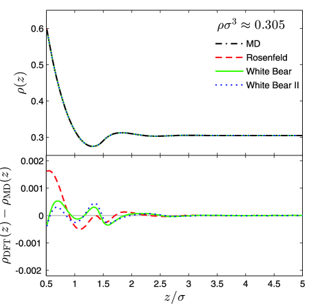
Figure 1: (Color online) Top panel: Equilibrium density profiles $\rho(z)$ of a hard-sphere fluid of reduced density $\rho^{*}\approx 0.305$ ($\eta\approx 0.159$) at a planar hard wall. The black line denotes data from MD simulation, while the red, green and blue lines correspond to various versions of FMT. Bottom panel: the deviation of the FMT densities from the MD results. The statistical errors in the MD data are smaller than the width of the lines.

At a somewhat larger value of the bulk density, $\rho^{*}\approx 0.701$ ($\eta\approx 0.367$) (shown in figure 2), the agreement between the profiles from FMT and those from computer simulations is very good in all details. At this intermediate bulk density, the PY and CS pressure differ by about 3%, which is reflected by a small deviation between the density profile obtained from the Rosenfeld functional and the profiles from the White Bear versions of FMT— especially close to the wall. This deviation, however, is sufficiently small that it can only be seen in the bottom panel of figure 2. Packing effects at this bulk density are significantly more pronounced than for the bulk density used for figure 1 — note the different scales for the $y$-axes in the bottom panel.

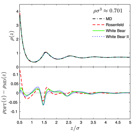
Figure 2: (Color online) Same as figure 1 for $\rho^{*}\approx 0.701$ ($\eta\approx 0.367$).

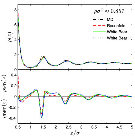
Figure 3: (Color online) Same as figure 1 for $\rho^{*}\approx 0.857$ ($\eta\approx 0.449$).

As the bulk density is further increased to $\rho^{*}\approx 0.857$ ($\eta\approx 0.449$) (figure 3), and $\rho^{*}\approx 0.938$ ($\eta\approx 0.492$) (figure 4), respectively, the agreement between FMT and computer simulations is still good very close to the wall, but clearly less satisfying for the oscillatory structure — we observe that the FMT significantly underestimates the height of the density peaks about one particle diameter away from the wall. Especially at $\rho^{*}\approx 0.938$, a density close to bulk freezing, one can see that the height of the second density peak is also underestimated by FMT.

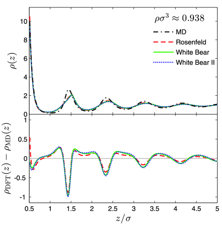
Figure 4: (Color online) Same as figure 1 for $\rho^{*}\approx 0.938$ ($\eta\approx 0.492$).

Since all versions of FMT seem to have a problem with the second peak in the density profile at high fluid density, it seems likely that it is not due to the precise form of the excess free energy density $\Phi$ employed, but rather the structure and range of the weight functions that can only approximate the complicated integrals of the virial expansion of the free energy [20, 21, 22].

3.2 Surface free energy $\gamma$

From the equilibrium density profile it is straightforward within DFT to compute the wall surface free energy from equation (2.4). Because various versions of FMT result in slightly different density profiles, as shown in figures 1–4, the wall surface free energy obtained from different versions of FMT are expected to differ by a small amount.

The MD simulation results were obtained, as in reference [2], using equation (2.8) and integrating the excess volume, $v_{\textrm{ex}}$, with respect to pressure. In that work, the numerical error in the integration was minimized by subtracting from the integrand the expression for the excess volume from Scaled Particle Theory (SPT) and then adding back, after integration, the exact expression for the SPT. For the data used in reference [2] this was sufficient to ensure that the numerical integration error was smaller than the reported statistical error. However, this is not sufficient for the high precision simulations reported here. To calculate $\gamma$ from the current MD results, instead of subtracting the SPT expression from the integrand, we subtract the corresponding expression from a recent high-accuracy parameterization of $\gamma$, presented in reference [23]. This results in a numerical error that is smaller than the reported statistical error. A table of numerical values of $\gamma$ is presented in the Supplementary Information [6].

In figure 5, we show a comparison of the wall surface free energy as a function of the packing fraction $\eta$ from different versions of FMT (lines) and from MD simulations (symbols). As expected, the agreement among different versions of FMT and the MD simulations is excellent at small and intermediate values of the packing fraction and remains good in the whole fluid density range.

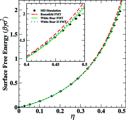
Figure 5: (Color online) The wall surface free energy $\gamma$ of a hard-sphere fluid at a planar hard wall as a function of the packing fraction $\eta$. The overall agreement between different versions of FMT (lines) and MD simulations (symbols) is excellent. For $\eta\geqslant 0.4$ there are small deviations between the DFT and MD results.

At higher values of the packing fraction, $\eta\geqslant 0.3$, one can observe that the FMT results slightly overestimate the wall surface free energy compared to the MD results [23]. In the inset, we highlight the region of high values of $\eta$, from which one can clearly see that the wall surface free energy obtained by the original Rosenfeld functional (red line) overestimates the values from the simulations the most, while the prediction from the White-Bear version of FMT (green line) is closest to the MD data.

Recently, a new parametrization of the simulation data for $\gamma$ was given by us [23], that is accurate in the whole range of fluid densities. Especially at higher densities, an additional term with a high power in $\eta$ is required in the parametrization in order to account for all the simulation data. Such a term is not reflected in the excess free energy density $\Phi$ of FMT.

3.3 Adsorption $\Gamma$ and excess volume $v_{\textrm{ex}}$

As discussed in section 2, the excess adsorption $\Gamma$ can be calculated via two different routes: (i) by integrating the density profile, equation (2.3), or (ii) using the adsorption theorem, equation (2.5). We have confirmed that our DFT and MD results are consistent, in that they yield the same values of $\Gamma$ via both routes. The MD data for $\Gamma$ can be found in the Supplemental Information [6].

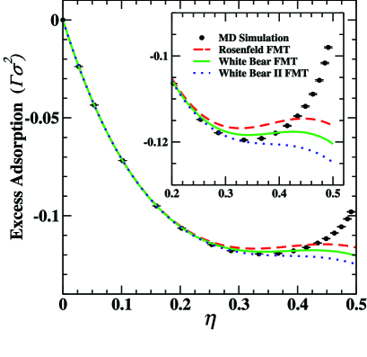
Figure 6: (Color online) The excess adsorption $\Gamma$ for a hard-sphere fluid at a planar hard wall as a function of the packing fraction $\eta$. The symbols denote data from MD simulation, while the lines correspond to different versions of FMT.

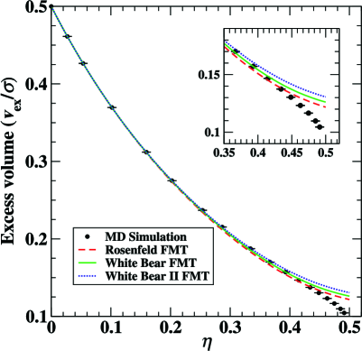
Figure 7: (Color online) The excess volume $v_{\textrm{ex}}$ for a hard-sphere fluid at a planar hard wall as a function of the packing fraction $\eta$. The symbols denote data from MD simulation, while the lines correspond to different versions of FMT.

In figure 6, we show the excess adsorption as a function of the packing fraction $\eta$. At low values of $\eta$, the DFT results are indistinguishable from each other and agree very well with the MD data. In contrast to the wall surface free energy $\gamma$, shown in figure 5, FMT results start to deviate from the MD data already at a moderate value of $\eta\geqslant 0.25$. For $\eta\geqslant 0.3$, the results from different versions of FMT begin to deviate from each other and for $\eta\geqslant 0.4$, there is a significant difference between the simulation results and those from FMT. While the excess adsorption increases towards less negative values for $\eta\geqslant 0.4$ in the simulation results, the FMT results display a local minimum and then decrease further for $\eta\to 0.5$. It should be noted that the presence of the local minimum is a consequence of the current choice of volume definition. If one uses another commonly used volume definition in which the position of the wall is coincident with the center of a hard sphere in contact with the wall then the local minimum disappears; however, the underestimation by the DFT of $\Gamma$ at high packing fractions remains.

The excess volume, $v_{\textrm{ex}}$ as a function of $\eta$ is shown in figure 7 — see the Supplemental Information[6] for numerical values of $v_{\textrm{ex}}(\eta)$ obtained from MD simulation. As is the case for $\Gamma$, there are significant deviations in the FMT estimates for $v_{\textrm{ex}}$ from the MD results at high packing fraction, $\eta>0.4$. At these high packing fractions, the values of $v_{\textrm{ex}}$ are overestimated by all versions of FMT examined. The excess volume has a direct relationship to the surface free energy through equation (2.8) and it is through the integration of this equation that the MD simulation values for $\gamma$ shown in figure 5 are calculated [2]. Because $v_{\textrm{ex}}$ is directly calculated from the density profile using equation (2.6), it provides a direct link between the density profile and interfacial thermodynamics, as measured by the surface free energy. In fact, the overestimation of $v_{\textrm{ex}}$ by the FMT at high packing fractions is dominated by a significant underestimation, at high $\eta$ by the FMT, of the second and third peaks of $\rho(z)$ (figure 3 and  4). Because the pressure is a monotonously increasing function of $\eta$, the overestimation of $v_{\textrm{ex}}$ at high packing fractions by the FMT leads directly, through equation (2.8) to the observed overestimation of $\gamma$ by the FMT.

4 Discussion

The overall agreement between the benchmark simulation data for the density profiles, the wall surface free energy and the excess adsorption of hard sphere fluid at a planar hard wall and the results obtained using accurate FMT DFT calculation is very good. We have found, however, that systematic deviations develop at sufficiently large packing fractions $\eta$. First, small deviations develop at around $\eta\geqslant 0.3$. They become more serious for $\eta\geqslant 0.4$ and show up in all quantities that we have studied here, i.e., the density profiles, the surface free energy and the excess adsorption. This was also observed in a study of confined hard-sphere fluids [24].

We find that for the dividing surface employed in our study, the actual hard wall position, the DFT results of the surface free energy $\gamma$ is less sensitive to the deviations in the density profiles than the excess adsorption $\Gamma$. While the deviation in $\gamma$ between the DFT and the simulation results is small, even at high packing fractions, the DFT results for $\Gamma$ show far larger relative deviations compared to the benchmark simulations. At the moment it is not clear whether these deviations can be reduced by changing the form of the excess free energy density $\Phi$ — the functional form of the empirical parametrization of $\gamma$ and $\Gamma$ [23] could give a hint — or if they are due to the range of weight functions employed by FMT.

Ukrainian 0

Твердi сфери бiля плоскої твердої стiни: моделювання та теорiя функцiоналу густини Р.Л. Давидчак${}^{\textsf{\footnotesize{\mbox{?}}}}$, Б.Б. Лейрд${}^{\textsf{\footnotesize{\mbox{?}}}}$, Р. Рот${}^{\textsf{\footnotesize{\mbox{?}}}}$

             
${}^{\textsf{\footnotesize 1}}$ Математичний факультет, Унiверситет Лестера, Лестер, LE1 7RH, Великобританiя ${}^{\textsf{\footnotesize 2}}$ Хiмiчний факультет, Унiверситет Канзасу, Лоуренс, Канзас 66045, США ${}^{\textsf{\footnotesize 3}}$ Iнститут теоретичної фiзики, Унiверситет Тюбiнґена, D-72074 Тюбiнґен, Нiмеччина

References

- [1] Laird B.B., Davidchack R.L., J. Phys. Chem., 2007, 111, 15935; doi:10.1063/1.1563248.
- [2] Laird B.B., Davidchack R.L., J. Chem. Phys., 2010, 132, 204101; doi:10.1063/1.3428383.
- [3] Rosenfeld Y., Phys. Rev. Lett., 1989, 63, 980; doi:10.1103/PhysRevLett.63.980.
- [4] Roth R., J. Phys.: Condens. Matter, 2010, 22, 063102; doi:10.1088/0953-8984/22/6/063102.
- [5] Rapaport D.C., The Art of Molecular Dynamics Simulation, 2nd Edn., Cambridge University Press, New York, 2004.
- [6] Supplementary data for this work can be found at http://hdl.handle.net/2381/33537.
- [7] Laird B.B., Hunter A., Davidchack R.L., Phys. Rev. E, 2012, 86, 060602(R); doi:10.1103/PhysRevE.86.060602.
- [8] Courtemanche D.J., van Swol F., Phys. Rev. Lett., 1992, 69 2078; doi:10.1103/PhysRevLett.69.2078.
- [9] Dijkstra M., Phys. Rev. Lett., 2004, 93, 108303; doi:10.1103/PhysRevLett.93.108303.
- [10] Auer S., Frenkel D., Phys. Rev. Lett., 2003, 91, 015703; doi:10.1103/PhysRevLett.91.015703.
- [11] Evans R., Adv. Phys., 1979, 28, 143; doi:10.1080/00018737900101365.
- [12] Bryk P., Roth R., Mecke K.R., Dietrich S., Phys. Rev. E, 2003, 68, 031602; doi:10.1209/epl/i2004-10410-4.
- [13] Roth R., Evans R., Lang A., Kahl G., J. Phys.: Condens. Matter, 2002, 14, 12063; doi:10.1088/0953-8984/14/46/313.
- [14] Yu Y.-X., Wu J., J. Chem. Phys., 2002, 117, 10156; doi:10.1063/1.1520530.
- [15] Hansen-Goos H., Roth R., J. Phys.: Condens. Matter, 2006, 18, 8413; doi:10.1088/0953-8984/18/37/002.
- [16] Mansoori G.A., Carnahan N.F., Starling K.E., Leland T.W. Jr., J. Chem. Phys., 1971, 54, 1523; doi:10.1063/1.1675048.
- [17] Hansen-Goos H., Roth R., J. Chem. Phys., 2006, 124, 154506; doi:10.1063/1.2187491.
- [18] Carnahan N.F., Starling K.E., J. Chem. Phys., 1969, 51, 635; doi:10.1063/1.1672048.
- [19] Boublík T., J. Chem. Phys., 1970, 53, 471; doi:10.1063/1.1673824.
- [20] Leithall G., Schmidt M., Phys. Rev. E, 2011, 83, 021201; doi:10.1103/PhysRevE.83.021201.
- [21] Korden S., Phys. Rev. E, 2012, 85, 041150; doi:10.1103/PhysRevE.85.041150.
- [22] Marechal M., Korden S., Mecke K., Phys. Rev. E, 2014, 90, 042131; doi:10.1103/PhysRevE.90.042131.
- [23] Davidchack R.L., Laird B.B., Roth R., Mol. Phys., 2015, 113, 1091; doi:10.1080/00268976.2014.986240.
-
[24]
Deb D., Winkler A., Yamani M.H., Oettel M.,
Virnau P., Binder K., J. Chem. Phys., 2011, 134, 214706;
doi:10.1063/1.3593197.
Ukrainian \adddialect\l@ukrainian0 \l@ukrainian