Polarized-Deuteron Stripping Reaction at Intermediate Energies

Abstract

A general analytical expressions for the cross-section and the polarization of nucleons arising in the inclusive deuteron stripping reaction have been derived in the diffraction approximation. The nucleon-nucleus phases were calculated in the framework of Glauber formalism and making use of the double-folding potential. The tabulated distributions of the target nucleus density and the realistic deuteron wave function with correct asymptotic at large nucleon-nucleon distances were used. The calculated angular dependences for the cross-sections and the analyzing powers of the $(\vec{d},p)$ reaction are in good agreement with corresponding experimental data.

I Introduction

Deuteron-induced nuclear reactions are widely used for studying the spectroscopic properties and the structure of nuclei. The importance of such reactions in experimental nuclear physics is associated with both the simplicity in obtaining monochromatic deuteron beams with the precisely calibrated polarization and a large yield of $dA$-reactions in comparison with reactions induced by other charged particles.

The majority of theoretical works on deuteron stripping reactions were published in 1950s–1970s. A surge of interest in those reactions, which has been observed in the last decade, was connected with intensive researches of radioactive nuclei with an excess of protons or neutrons near the stability valley. In those reactions, besides the emergence of a residual nucleus in the bound state, the formation of resonant states also becomes probable muk11 . This circumstance makes the nucleon-transfer reactions a unique tool for studying unstable nuclei and astrophysical reactions of the $(N,\gamma)$ and $(p,\alpha)$ types.

In this work, the inclusive deuteron stripping reaction was considered. Its formalism for the case of intermediate energies was proposed for the first time by Serber ser47 and developed in works by Akhiezer and Sitenko akh57 ; sit90 . In work kov15 , it was shown that the multiple integral in the expression for the reaction cross-section sit90 can be calculated analytically by expanding the integrands in the basis of Gaussoid functions. The scattering phases were calculated at that in the framework of Glauber formalism, making use of the double folding potential cha90 ; shu01 and the tabulated distributions of the target nucleus density vri87 . Therefore, the final result (the cross-section) depended on a single parameter corresponding to the normalization of the imaginary part of nucleon-nucleus potential. This approach was used to describe the differential cross-sections of ²H$(d,n)^{3}$He reaction wil80 at relativistic energies of incident deuterons. The application of the deuteron wave function with a correct asymptotic at large distances between nucleons was shown to be important at calculations.

By continuing work kov15 , in this work, a more complicated problem was considered; namely, the calculation of observables for the inclusive polarized-deuteron stripping reaction. The microscopic description for the distributions of nucleon density and scattering phases was also introduced. This procedure made it possible to keep the number of fitting parameters to a minimum and, in such a manner, to obtain a quantitative description of the experiment. Besides, the model itself and the limits of its applicability to the kinematics of the reaction concerned were verified. Notice that, in this approach, the reaction density matrix is a five-fold integral only formally, because the profile functions, which the density matrix depends on, are also expressed in terms of multiple integrals. Therefore, generally speaking, we have rather a complicated computational problem.

Nevertheless, as will be shown below, the final formulas for the cross-section and analyzing power can be reduced to algebraic expressions, namely, multiple sums of elementary functions, if Gaussoid functions are used as integrands. Notice that a similar trick is applied rather often: in the variational approach to the description of bound states kuk77 ; var95 ; gri00 , for the parametrization of nuclear charge densities in the ground state of nucleus sic74 , and in scattering problems dal85 , which makes it possible to calculate the corresponding scattering phases and form factors analytically.

The structure of the paper is as follows. Section II is devoted to the description of formalism applied while calculating the angular (energy) distributions of cross-sections and polarizations for nucleons that arise in the deuteron stripping reaction. In Section III, the results of numerical calculations for the differential cross-sections and analyzing powers are discussed and compared with corresponding experimental data. Section IV contains conclusions. The most important auxiliary formulas used to simplify the formalism description are given in Appendices.

II Formalism

Light and medium nuclei were selected as targets, because in this case and in the case of intermediate energies, the Coulomb interaction can be neglected.

Let a proton be a particle that arises in the deuteron stripping reaction. The angular distribution of protons arising in the reaction $(\vec{d},p)$ is described by the formula sat83

$$d\sigma/d\Omega=(1+3\mathbf{P}_{d}\mathbf{P})(d\sigma/d\Omega)_{0}\,,$$ (1)

where $\mathbf{P}_{d}$ is the polarization of incident deuterons, and $\mathbf{P}$ the polarization of protons arising in the non-polarized deuteron stripping reaction. The cross-section for the latter reaction equals $(d\sigma/d\Omega)_{0}$. The quantity $\mathbf{P}$ is defined in terms of the density matrix $\rho$ as follows sit12 :

$$\mathbf{P}=\frac{\text{Tr\thinspace}({\bm{\sigma}}\rho)}{\text{Tr\thinspace}\rho}\,,$$ (2)

where $\bm{\sigma}$ are Pauli’s matrices.

Let the deuteron move in the positive direction of $z$-axis in the Cartesian coordinate system, so that the $xy$-plane is the impact parameter plane. The proton and neutron of the deuteron will be designated by subscripts 1 and 2, respectively. In the diffraction approximation, the general expression for the density matrix of stripping reaction looks like sit90

$$\rho(\mathbf{k}_{1})=\int d\mathbf{b}_{2}(1-|1-\Omega_{2}|^{\,2})a_{\mathbf{k}_{1}}(\mathbf{r}_{2})a_{\mathbf{k}_{1}}^{\dagger}(\mathbf{r}_{2}),$$ (3)

where $\mathbf{b}_{2}$ is the neutron impact parameter vector, $\Omega_{2}$ the corresponding profile function; the quantity

$$a_{\mathbf{k}_{1}}(\mathbf{r}_{2})=\int d\mathbf{r}_{1}\exp(-i\mathbf{k}_{1}\mathbf{r}_{1})(1-\Omega_{1})\varphi_{0}(\mathbf{r}),\quad\mathbf{r}=\mathbf{r}_{1}-\mathbf{r}_{2},$$ (4)

is the probability amplitude that the proton has the momentum $\mathbf{k}_{1}$ and the neutron is located at the point $\mathbf{r}_{2}$, and $\varphi_{0}(\mathbf{r})$ is the deuteron wave function. The neutron profile function $\Omega_{2}$ in (3) contains only the radial part, i.e. $\Omega_{2}(b_{2})=\omega_{2}(b_{2})$, whereas the proton one, ${\Omega}_{1}$, depends also on the spin sit58 :

$${\Omega}_{1}(\mathbf{r}_{1})=\omega_{1}(b_{1})\{1+i\gamma_{1}\exp(i\delta_{1}){\bm{\sigma}}((\mathbf{k}/2)\times\partial/\partial\mathbf{r}_{1})\},$$ (5)

where $b_{1}$, $\gamma_{1}$, and $\delta_{1}$ are the impact parameter, the constant of spin-orbit interaction between the proton and the nucleus, and the phase shift, respectively; and $\mathbf{k}$ is the vector of the incident deuteron momentum.

If the integrand in (3) includes Gaussian functions, the density matrix can be calculated explicitly. Without loss of generality, let us expand the functions $\omega_{i}(b_{i})$ and $\varphi_{0}(\mathbf{r})$ in series of Gaussoid basis functions,

$$\omega_{i}(b_{i})=\sum\limits_{j=1}^{N}{\alpha_{ij}}\exp(-b_{i}^{2}/\beta_{ij}),$$ (6)

$$\varphi_{0}(\mathbf{r})=\sum\limits_{j=1}^{N}{c_{j}}\exp(-d_{j}|\mathbf{r}_{1}-\mathbf{r}_{2}|^{2}),$$ (7)

where $\beta_{ij}=R_{rms}^{2}/j$, and $R_{rms}$ is the root-mean-square radius of target nucleus.

Analytical integration in (3) with functions (6) and (7), and the calculation of the traces of corresponding matrices in the numerator and denominator of formula (2) bring us to the expressions $\mathrm{Tr\,}({\bm{\sigma}}\rho(\mathbf{k}_{1}))=\mathbf{G}(\mathbf{k}_{1})$ and $\mathrm{Tr}\,\rho(\mathbf{k}_{1})=H(\mathbf{k}_{1})$ (see Appendix A). Therefore, the proton polarization is determined by the formula

$$\mathbf{P}(\mathbf{k}_{1})=\frac{G(\mathbf{k}_{1})}{H(\mathbf{k}_{1})}({\bm{\kappa}}_{1}\!\times\!{\mathbf{k}_{1}})\,,$$ (8)

where ${\bm{\kappa}}_{1}$ is the transverse component of the momentum $\mathbf{k}_{1}=\left\{{\bm{\kappa}}_{1},(\mathbf{k}/k)k_{1z}\right\}$. The magnitudes $\kappa_{1}$ and $k_{1z}$ of the $\mathbf{k}_{1}$-vector components are related to the proton energy $T_{1}$ and the proton emission angle $\Theta_{1}$ in the laboratory frame by the relationships sit90

$$\kappa_{1}=(k/2+k_{1z})\tan\Theta_{1},$$ (9)

$$k_{1z}=\sqrt{m/T}(T_{1}-T/2),$$ (10)

where $m$ is the nucleon mass, and $T$ the initial energy of deuteron.

The cross-section of non-polarized-deuteron stripping reaction, after which the wave vector of emitted proton falls within the interval $d\mathbf{k}_{1}$, is determined by the denominator in (8):

$$d\sigma_{0}=H(\mathbf{k}_{1})\frac{d\mathbf{k}_{1}}{(2\pi)^{3}}.$$ (11)

In order to find the dependences of polarization (8) and cross-section (11) on the proton emission angle, the expression obtained for $G(\mathbf{k}_{1})$ and $H(\mathbf{k}_{1})$ have to be integrated over the $z$-component of vector $\mathbf{k}_{1}$ sit90 . By expressing the components of $d\mathbf{k}_{1}$ in the cylindrical coordinate system and taking into account (9), we obtain

$$P(\Theta_{1})=\frac{\widetilde{G}(\kappa_{1})}{\widetilde{H}(\kappa_{1})}\,,\quad\sigma_{0}(\Theta_{1})=\frac{\widetilde{H}(\kappa_{1})}{(2\pi)^{3}\cos^{3}\Theta_{1}}\,,$$ (12)

where

$$\widetilde{G}(\kappa_{1})=\int_{-\infty}^{\infty}(k/2+k_{1z})^{2}G(\kappa_{1},k_{1z})dk_{1z}\,,$$ (13)

$$\widetilde{H}(\kappa_{1})=\int_{-\infty}^{\infty}(k/2+k_{1z})^{2}H(\kappa_{1},k_{1z})dk_{1z}\,.$$ (14)

Cross-section (12) and the angle $\Theta_{1}$ were transformed into their counterparts in the center-of-mass system making use of kinematic relations from work bal63 .

III Calculation results and their discussion

The formalism described in the previous section was applied to analyze experimental data (the cross-section and the analyzing power) obtained for $(\vec{d},p)$ stripping reactions on the ${}^{24}\text{Mg}$ and ${}^{40}\text{Ca}$ nuclei at the deuteron energy $T=56$ MeV hat84 ; uoz94 .

When expanding the wave function $\varphi_{0}(\mathbf{r})$ in series (7), tabulated data for the S-component of deuteron wave function obtained with the help of realistic $NN$-potential Nijm I sto94 were used.

The profile functions $\omega_{i}(b_{i})$, which were expanded in series (6), were first calculated in the eikonal approximation (see Appendix B) making use of the tabulated nuclear density distributions for the ${}^{24}\text{Mg}$ and ${}^{40}\text{Ca}$ nuclei taken from work vri87 . The number $N$ of terms in expansions (6) and (7) was taken to equal 12.

The values of spin-orbit parameters in (5) were determined from the relations sit90

$$\delta_{1}=\arctan(W_{0}/V_{0}),\quad\gamma_{1}=V_{\text{so}}r_{\text{so}}^{2}/(2\sqrt{V_{0}^{2}+W_{0}^{2}}),$$ (15)

where $V_{0}$, $W_{0}$, $V_{\text{so}}$, and $r_{\text{so}}$ are the relevant parameters for the central and spin-orbit parts of the nucleon-nucleus optical potential. From the data of work bor69 ; fab80 , it follows that, for the proton energy ${T_{1}=T/2=28}$ MeV, the parameters $\delta_{1}$ and $\gamma_{1}$ are equal to 0.12 and 0.07, respectively, for the ²⁴Mg target nucleus, and to 0.13 and 0.08, respectively, for ⁴⁰Ca.

The coefficients in expansions (6) and (7) together with quantities (15) were used to calculate the angular distribution of protons,

$$\sigma(\theta)=[1+3P_{d}P(\theta)]\sigma_{0}(\theta),$$ (16)

where $P(\theta)$ and $\sigma_{0}(\theta)$ are the polarization and cross-section (12) in the center-of-mass system. The polarization of deuteron beam, $P_{d}$, amounted to about 0.5 hat84 or 0.52 uoz94 .

In Fig. 1, cross-sections (16) and analyzing powers ${A}_{y}(\theta)=2P(\theta)$ yul68 calculated for polarized-deuteron stripping reactions on the ${}^{24}\text{Mg}$ and ${}^{40}\text{Ca }$ nuclei at $T=56$ MeV are depicted by solid curves. The dashed curves were obtained for the model function

$$\varphi_{0}(\mathbf{r})=(2\xi/\pi)^{3/4}\exp(-\xi|\mathbf{r}_{1}-\mathbf{r}_{2}|^{2}).$$ (17)

The value of the parameter $\xi$ was selected to equal $\xi=0.049$ fm^-2, at which formula (17) reproduced the experimental mean-square radius of deuteron mus92 . The dash-dotted curves correspond to the results of calculations carried out in works hat84 ; uoz94 for the quantities $\sigma(\theta)$ and $A_{y}(\theta)$ in the framework of the adiabatic distorted wave approximation jsp70 .

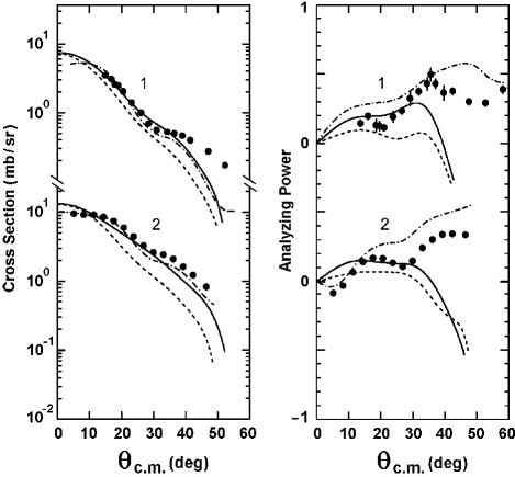
Figure 1: Angular dependences of cross-sections (left panel) and analyzing powers (right panel) for $(\vec{d},p)$ stripping reactions on the ${}^{24}\text{Mg}$ (1) and ${}^{40}\text{Ca}$ (2) nuclei at a deuteron energy of 56 MeV. See further explanations in the text. Experimental data were taken from works hat84 ; uoz94 .

The experimental data were fitted using a single fitting parameter $N_{W}$, the normalization parameter for the imaginary part of double folding potential (see Appendix B). Its values amounted to 0.24 for the ²⁴Mg target nucleus and 0.19 for ⁴⁰Ca. By varying the parameter $N_{W}$, the both dependences, $\sigma(\theta)$ and $A_{y}(\theta)$, were fitted simultaneously to the relevant experimental data. The parameter $N_{W}$ was found to affect the shape of the curve $A_{y}(\theta)$, but not the slope of the linear section in the dependence $\sigma(\theta)$.

Direct nuclear reactions, including the stripping one, are surface reactions sat83 . Therefore, the calculated observable quantities are expected to be sensitive to the asymptotics of the wave functions of interacting particles, which is confirmed by specific calculations. From Fig. 1, one can see that deuteron model function (17), which has an incorrect asymptotic at large nucleon-nucleon distances, does not allow the cross-sections and analyzing powers to be described adequately (the dashed curves).

Notice that the deuteron stripping problem considered above was solved here exactly, making no additional simplifications and restrictions, which could affect the result of numerical calculation. From the analysis of the behavior of solid curves in Fig. 1, it follows that the calculation results satisfactorily describe the corresponding experimental data for the angles $\theta<(30\div 35)^{\circ}$. Therefore, in the case of the incident deuteron energy $T=56$ MeV and the ${}^{24}\text{Mg}$ and ${}^{40}\text{Ca target }$nuclei, the applicability region of diffraction approximation for the description of $(\vec{d},p)$ reaction is confined to the indicated interval of proton emission angles.

IV Conclusions

The main result of this work includes general expressions (Appendix A) that allow the cross-sections and the analyzing powers of the inclusive polarized-deuteron stripping reaction to be calculated. The formulas were obtained in the diffraction approximation by analytically integrating the expression for the corresponding density matrix. This approach can also be applied in other similar problems with multiple integrals if the integrand allows an expansion in a series of Gaussoid basis functions.

With the help of tabulated data for the densities of target nuclei and making use of a realistic deuteron wave function with a correct asymptotic at large nucleon-nucleon distances, the observed angular dependences of the cross-sections and analyzing powers for the $(\vec{d},p)$ reaction were described in the case of ${}^{24}\text{Mg}$ and ${}^{40}\text{Ca target}$ nuclei and a deuteron energy of 56 MeV. A single fitting parameter was used at that, namely, the normalization parameter for the imaginary part of the high-energy double folding potential.

It should be noticed that the general formulas obtained in this work can be used to describe the cross-sections and polarizations not only for the inclusive processes of deuteron stripping, but also deuteron, as well as light- and heavy-ion, breakup uts85 . Both the angular and energy distributions of indicated quantities can be calculated. In the latter case, expressions for $G$ and $H$ in (8) and (11) should be integrated over the normal components of the emitted particle momentum.

Appendix A Traces of the density matrix $\rho$ and the products ${\bm{\sigma}}\rho$

In this Appendix, the calculation results are presented for the traces of the matrices in the numerator and denominator of expression (2) after analytical integration in (3) with functions (6) and (7).

The numerator in (2) looks like

$$\text{Tr}\,({\bm{\sigma}}\rho(\mathbf{k}_{1}))=\mathbf{G}(\mathbf{k}_{1})=G(\mathbf{k}_{1})({\bm{\kappa}}_{1}\!\times\!{\mathbf{k}_{1}})\,.$$ (18)

Here, ${\bm{\kappa}}_{1}$ is the transverse component of emitted particle momentum $\mathbf{k}_{1}=\left\{{\bm{\kappa}}_{1},\mathbf{k}_{1z}\right\}$, and the quantity $G(\mathbf{k}_{1})$ is defined as follows:

$$G(\mathbf{k}_{1})=\gamma_{1}\sin\delta_{1}\sum\limits_{p=1}^{N}\sum\limits_{q=1}^{N}{c_{p}}{c_{q}}Z(\lambda,\kappa_{1},k_{1z}),$$ (19)

where

$$Z(\lambda,\kappa_{1},k_{1z})=2\lambda t(\lambda,k_{1z})(4z^{(1)}(\lambda,\kappa_{1})-z^{(2)}(\lambda,\kappa_{1})),$$ (20)

$$z^{(1)}(\lambda,\kappa_{1})=z_{11}(\lambda,\kappa_{1})-z_{12}(\lambda,\kappa_{1}),$$ (21)

$$z^{(2)}(\lambda,\kappa_{1})=4z_{21}(\lambda,\kappa_{1})+z_{22}(\lambda,\kappa_{1}).$$ (22)

The denominator in (2) is determined by the formula

$$\text{Tr}\,\rho(\mathbf{k}_{1})=H(\mathbf{k}_{1})=H_{0}(\mathbf{k}_{1})+\gamma_{1}^{2}H_{\text{so}}(\mathbf{k}_{1})\,,$$ (23)

where

$$H_{0}(\mathbf{k}_{1})=\sum\limits_{p=1}^{N}\sum\limits_{q=1}^{N}{c_{p}}{c_{q}}Y(\lambda,\kappa_{1},k_{1z}),$$ (24)

$$Y(\lambda,\kappa_{1},k_{1z})=t(\lambda,k_{1z})(y^{(1)}(\lambda,\kappa_{1})-y^{(2)}(\lambda,\kappa_{1})),$$ (25)

$$y^{(1)}(\lambda,\kappa_{1})=4(y_{11}(\lambda,\kappa_{1})-2y_{12}(\lambda,\kappa_{1})+y_{13}(\lambda,\kappa_{1})),$$ (26)

$$y^{(2)}(\lambda,\kappa_{1})=y_{21}(\lambda,\kappa_{1})-4y_{22}(\lambda,\kappa_{1})+y_{23}(\lambda,\kappa_{1});$$ (27)

$$H_{\text{so}}(\mathbf{k}_{1})=\sum\limits_{p=1}^{N}\sum\limits_{q=1}^{N}{c_{p}}{c_{q}}W(\lambda,\kappa_{1},k_{1z}),$$ (28)

$$W(\lambda,\kappa_{1},k_{1z})=\,\, t(\lambda,k_{1z})(4w^{(1)}(\lambda,\kappa_{1},k_{1z})$$ (29)

$$-w^{(2)}(\lambda,\kappa_{1},k_{1z})),$$

$$w^{(1)}(\lambda,\kappa_{1},k_{1z})=w_{11}(\lambda,\kappa_{1},k_{1z})+2w_{12}(\lambda,\kappa_{1},k_{1z}),$$ (30)

$$w^{(2)}(\lambda,\kappa_{1},k_{1z})=w_{21}(\lambda,\kappa_{1},k_{1z})+w_{22}(\lambda,\kappa_{1},k_{1z}).$$ (31)

The values in right sides of (21), (22), (26), (27), (30), and (31) are defined as follows:

$$z_{11}(\lambda,\kappa_{1})=\sum\limits_{i=1}^{N}\sum\limits_{j=1}^{N}\frac{\alpha_{1i}\beta_{1i}\,\alpha_{2j}\beta_{2j}}{(\lambda+\beta_{1i}+\beta_{2j})^{2}}\exp\Bigl{(}-\frac{\lambda+2\beta_{1i}+2\beta_{2j}}{\lambda+\beta_{1i}+\beta_{2j}}\,\frac{\lambda\kappa_{1}^{2}}{4}\Bigr{)},$$ (32)

$$z_{12}(\lambda,\kappa_{1})=\sum\limits_{i=1}^{N}\sum\limits_{j=1}^{N}\sum\limits_{l=1}^{N}\frac{\alpha_{1i}\beta_{1i}\,\alpha_{1j}\beta_{1j}\,\alpha_{2l}\,\beta_{2l}}{(\lambda+\beta_{1ij})^{2}(\lambda+\beta_{1ij}+2\beta_{2l})}\exp\Bigl{(}-\frac{\beta_{1ij}}{\lambda+\beta_{1ij}}\,\frac{\lambda\kappa_{1}^{2}}{2}\Bigr{)},$$ (33)

$$z_{21}(\lambda,\kappa_{1})=\sum\limits_{i=1}^{N}\sum\limits_{j=1}^{N}\sum\limits_{l=1}^{N}\frac{\alpha_{1i}\beta_{1i}\,\alpha_{2j}\,\alpha_{2l}\beta_{2jl}}{(2\lambda+2\beta_{1i}+\beta_{2jl})^{2}}\exp\Bigl{(}-\frac{\lambda+2\beta_{1i}+\beta_{2jl}}{2\lambda+2\beta_{1i}+\beta_{2jl}}\,\frac{\lambda\kappa_{1}^{2}}{2}\Bigr{)},$$ (34)

$$z_{22}(\lambda,\kappa_{1})=\sum\limits_{i=1}^{N}\sum\limits_{j=1}^{N}\sum\limits_{l=1}^{N}\sum\limits_{n=1}^{N}\frac{\alpha_{1i}\beta_{1i}\,\alpha_{1j}\beta_{1j}\,\alpha_{2l}\alpha_{2n}\beta_{2ln}}{(\lambda+\beta_{1ij})^{2}(\lambda+\beta_{1ij}+\beta_{2ln})}\exp\Bigl{(}-\frac{\beta_{1ij}}{\lambda+\beta_{1ij}}\,\frac{\lambda\kappa_{1}^{2}}{2}\Bigr{)};$$ (35)

$$y_{11}(\lambda,\kappa_{1})=\exp\Bigl{(}-\frac{\lambda\kappa^{2}_{1}}{2}\Bigr{)}\sum\limits_{i=1}^{N}\alpha_{2i}\beta_{2i},$$ (36)

$$y_{12}(\lambda,\kappa_{1})=\sum\limits_{i=1}^{N}\sum\limits_{j=1}^{N}\frac{\alpha_{1i}\beta_{1i}\,\alpha_{2j}\beta_{2j}}{\lambda+\beta_{1i}+\beta_{2j}}\exp\Bigl{(}-\frac{\lambda+2\beta_{1i}+2\beta_{2j}}{\lambda+\beta_{1i}+\beta_{2j}}\,\frac{\lambda\kappa^{2}_{1}}{4}\Bigr{)},$$ (37)

$$y_{13}(\lambda,\kappa_{1})=\sum\limits_{i=1}^{N}\sum\limits_{j=1}^{N}\sum\limits_{l=1}^{N}\frac{\alpha_{1i}\beta_{1i}\,\alpha_{1j}\beta_{1j}\,\alpha_{2l}\beta_{2l}}{(\lambda+\beta_{1ij})(\lambda+\beta_{1ij}+2\beta_{2l})}\exp\Bigl{(}-\frac{\beta_{1ij}}{\lambda+\beta_{1ij}}\,\frac{\lambda\kappa^{2}_{1}}{2}\Bigr{)},$$ (38)

$$y_{21}(\lambda,\kappa_{1})=\exp\Bigl{(}-\frac{\lambda\kappa^{2}_{1}}{2}\Bigr{)}\sum\limits_{i=1}^{N}\sum\limits_{j=1}^{N}\alpha_{2i}\beta_{2i}\,\beta_{2ij},$$ (39)

$$y_{22}(\lambda,\kappa_{1})=\sum\limits_{i=1}^{N}\sum\limits_{j=1}^{N}\sum\limits_{l=1}^{N}\frac{\alpha_{1i}\beta_{1i}\,\alpha_{2j}\beta_{2j}\,\beta_{2jl}}{2\lambda+2\beta_{1i}+\beta_{2jl}}\exp\Bigl{(}-\frac{\lambda+2\beta_{1i}+\beta_{2jl}}{2\lambda+2\beta_{1i}+\beta_{2jl}}\,\frac{\lambda\kappa^{2}_{1}}{2}\Bigr{)},$$ (40)

$$y_{23}(\lambda,\kappa_{1})=\sum\limits_{i=1}^{N}\sum\limits_{j=1}^{N}\sum\limits_{l=1}^{N}\sum\limits_{n=1}^{N}\frac{a_{1i}\beta_{1i}\,a_{1j}\beta_{1j}\,a_{2l}\beta_{2l}\,\beta_{2ln}}{(\lambda+\beta_{1ij})(\lambda+\beta_{1ij}+\beta_{2ln})}\exp\Bigl{(}-\frac{\beta_{1ij}}{\lambda+\beta_{1ij}}\,\frac{\lambda\kappa^{2}_{1}}{2}\Bigr{)};$$ (41)

$$w_{11}(\lambda,\kappa_{1},k_{1z})=\lambda^{2}\kappa^{2}_{1}k^{2}_{1z}\sum\limits_{i=1}^{N}\sum\limits_{j=1}^{N}\sum\limits_{l=1}^{N}\frac{\alpha_{1i}\beta_{1i}\,\alpha_{1j}\beta_{1j}\,\alpha_{2l}\beta_{2l}}{(\lambda+\beta_{1ij})^{3}(\lambda+\beta_{1ij}+2\beta_{2l})}\exp\Bigl{(}-\frac{\beta_{1ij}}{\lambda+\beta_{1ij}}\,\frac{\lambda\kappa_{1}^{2}}{2}\Bigr{)},$$ (42)

$$w_{12}(\lambda,\kappa_{1},k_{1z})=(2k_{1z}^{2}+\kappa_{1}^{2})\sum\limits_{i=1}^{N}\sum\limits_{j=1}^{N}\sum\limits_{l=1}^{N}\frac{\alpha_{1i}\beta_{1i}\,\alpha_{1j}\beta_{1j}\,\alpha_{2l}\,\beta_{2l}^{2}}{(\lambda+\beta_{1ij})^{2}(\lambda+\beta_{1ij}+2\beta_{2l})^{2}}\exp\Bigl{(}-\frac{\beta_{1ij}}{\lambda+\beta_{1ij}}\,\frac{\lambda\kappa_{1}^{2}}{2}\Bigr{)},$$ (43)

$$w_{21}(\lambda,\kappa_{1},k_{1z})=\lambda^{2}\kappa^{2}_{1}k^{2}_{1z}\sum\limits_{i=1}^{N}\sum\limits_{j=1}^{N}\sum\limits_{l=1}^{N}\sum\limits_{n=1}^{N}\frac{\alpha_{1i}\beta_{1i}\,\alpha_{1j}\beta_{1j}\,\alpha_{2l}\alpha_{2n}\beta_{2ln}}{(\lambda+\beta_{1ij})^{3}(\lambda+\beta_{1ij}+\beta_{2ln})}\exp\Bigl{(}-\frac{\beta_{1ij}}{\lambda+\beta_{1ij}}\,\frac{\lambda\kappa_{1}^{2}}{2}\Bigr{)},$$ (44)

$$w_{22}(\lambda,\kappa_{1},k_{1z})=(2k_{1z}^{2}+\kappa_{1}^{2})\sum\limits_{i=1}^{N}\sum\limits_{j=1}^{N}\sum\limits_{l=1}^{N}\sum\limits_{n=1}^{N}\frac{\alpha_{1i}\beta_{1i}\,\alpha_{1j}\beta_{1j}\,\alpha_{2l}\alpha_{2n}\beta_{2ln}^{2}}{(\lambda+\beta_{1ij})^{2}(\lambda+\beta_{1ij}+\beta_{2ln})^{2}}\exp\Bigl{(}-\frac{\beta_{1ij}}{\lambda+\beta_{1ij}}\,\frac{\lambda\kappa_{1}^{2}}{2}\Bigr{)}.$$ (45)

In (19), (24), and (28), $\lambda=2/(d_{p}+d_{q})$. The function $t(\lambda,k_{1z})$ in (20), (25), and (29) looks like

$$t(\lambda,k_{1z})=\pi^{4}\lambda^{3}\exp\left(-\frac{\lambda k_{1z}^{2}}{2}\right).$$ (46)

Besides,

$$\beta_{ijl}=2\beta_{ij}\beta_{il}/(\beta_{ij}+\beta_{il}),\quad(i\!=\!1,2;\,\,\,j,l\!=\!\overline{1,N}).$$ (47)

Appendix B Calculation of profile functions

The radial parts of nucleon-nucleus profile functions were calculated in the eikonal approximation:

$$\omega_{i}(b_{i})=1-\exp[-\phi_{i}(b_{i})],\quad i\!=\!1,2;$$ (48)

where

$$\phi_{i}(b_{i})=-\frac{1}{v}\int_{-\infty}^{\infty}dz\,W\left(\sqrt{b_{i}^{2}+z^{2}}\right)$$ (49)

is the scattering phase, $v$ the velocity of incident nucleon, and $W(r)$ the imaginary part of nucleon-nucleus potential.

In the framework of the double folding model, the eikonal phase can be calculated using the method described in work cha90 . Let the distribution of nuclear density in the nucleon, $\rho_{i}(r)$, and the amplitude of $NN$-interaction at the impact parameter plane, $f(b)$, be defined by Gaussian functions:

$$\rho_{i}(r)=\rho_{i}(0)\exp(-r^{2}/a_{i}^{2}),$$ (50)

$$f(b)=(\pi r_{0}^{2})^{-1}\exp(-b^{2}/r_{0}^{2}),$$ (51)

where $\rho_{i}(0)=(a_{i}\sqrt{\pi})^{-3}$, $a_{i}^{2}=r_{0}^{2}=2r_{NN}^{2}/3$, and $r_{NN}^{2}\cong~{}0.65~{}\mathrm{fm}^{2}$ is the mean-square radius of $NN$-interaction. If the density distribution (tabulated vri87 or model) in the target nucleus can be expanded in a series of Gaussoid basis functions,

$$\rho_{T}(r)=\sum_{j=1}^{N}\rho_{Tj}\exp(-r^{2}/a_{Tj}^{2}),\quad a_{Tj}^{2}=R_{rms}^{2}/j\,,$$ (52)

where $R_{rms}$ is the root-mean-square radius of the nucleus, the formula for the eikonal phase from work cha90 can be generalized kov15 to the expression

$$\phi_{i}(b_{i})=N_{W}\sqrt{\pi}\,\bar{\sigma}_{NN}\sum_{j=1}^{N}\frac{\rho_{Tj}\,a_{Tj}^{3}}{a_{Tj}^{2}+2r_{0}^{2}}\exp\left(-\frac{b_{i}^{2}}{a_{Tj}^{2}+2r_{0}^{2}}\right),$$ (53)

where $N_{W}$ is the normalization factor for the imaginary part of the double folding potential, and $\bar{\sigma}_{NN}$ is the isotopically averaged cross-section of nucleon-nucleon interaction shu01 .

Formula (53) was used directly while calculating profile functions (48). Afterwards, they were expanded in the Gaussoid basis (see (6)).

References

• (1) A. M. Mukhamedzhanov, Phys. Rev. C 84, 044616 (2011).
• (2) R. Serber, Phys. Rev. 72, 1008 (1947).
• (3) A. I. Akhiezer and A. G. Sitenko, Zh. Eksp. Teor. Fiz. 32, 1040 (1957) [Sov. Phys. JETP 6, 799 (1958)].
• (4) A. G. Sitenko, Theory of Nuclear Reactions, (World Scientific, Singapore, 1990), Chap. 4.
• (5) V. I. Kovalchuk, Nucl. Phys. A 937, 59 (2015).
• (6) S. K. Charagi and S. K. Gupta, Phys. Rev. C 41 1610 (1990).
• (7) P. Shukla, arXiv: nucl-th/0112039.
• (8) H. De Vries, C. W. De Jager, and C. De Vries, At. Data Nucl. Data Tables 36, 495 (1987).
• (9) C. Wilkin, J. Phys. G 6 69 (1980).
• (10) V. I. Kukulin and V. M. Krasnopol’sky, J. Phys. G. 3, 795 (1977).
• (11) K. Varga and Y. Suzuki, Phys. Rev. C 52, 2885 (1995).
• (12) B. E. Grinyuk, I. V. Simenog, Ukr. J. Phys. 45, 21 (2000).
• (13) I. Sick, Nucl. Phys. A 218, 509 (1974).
• (14) O. D. Dalkarov and V. A. Karmanov, Nucl. Phys. A 445, 579 (1985).
• (15) G. R. Satchler, Direct Nuclear Reactions, (Oxford Univ. Press, Oxford, 1983).
• (16) A. G. Sitenko, Scattering Theory, (Springer-Verlag Berlin Heidelberg, 2012).
• (17) A. G. Sitenko, Nucl. Phys. 9, 412 (1958/59).
• (18) A. M. Baldin, W. I. Goldanskij, and I. L. Rosental, Kinematik der Kernreaktionen, (Akad.-Verl., Berlin, 1963).
• (19) K. Hatanaka et al., Nucl. Phys. A 419, 530 (1984).
• (20) Y. Uozumi et al., Phys. Rev. C 50, 263 (1994).
• (21) V. G. J. Stoks, R. A. M. Klomp, C. P. F. Terheggen, and J. J. de Swart, Phys. Rev. C 49, 2950 (1994); http://nn-online.org.
• (22) A. Bohr, B. R. Mottelson, Nuclear Structure. Vol. I. Single-Particle Motion, (W. A. Benjamin Inc., New York, Amsterdam, 1969).
• (23) E. Fabrici et al., Phys. Rev. C 21, 830 (1980).
• (24) T. J. Yule and W. Haeberli, Nucl. Phys. A 117, 1 (1968).
• (25) M. M. Mustafa et al., Phys. Rev. C 45, 2603 (1992).
• (26) R. C. Johnson and P. J. R. Soper, Phys. Rev. C 1, 976 (1970).
• (27) H. Utsunomiya, Phys. Rev. C 32, 849 (1985).