Low Temperature Thermal Hall Conductivity of a Nodal Chiral Superconductor

Abstract

Motivated by Sr₂RuO₄, we consider a chiral superconductor where the gap is strongly suppressed along certain momentum directions. We evaluate the thermal Hall conductivity in the gapless regime, i.e., at temperature small compared with the impurity band width $\gamma$, taking the simplest model of isotropic impurity scattering. We find that, under favorable circumstances, this thermal Hall conductivity can be quite significant, and is smaller than the diagonal component (the universal thermal conductivity) only by a factor of $1/\ln(2\Delta_{M}/\gamma)$, where $\Delta_{M}$ is the maximum gap.

1 Introduction

Impurities play a dual role in transport properties of unconventional superconductors. They scatter the carriers responsible for the transport. This effect decreases the transport coefficients. On the other hand, impurities are pair-breaking and so generate new excitations which contribute to the transport. Under suitable circumstances, these two effects exactly cancel with each other and give rise to universal transport coefficients, independent of the concentration or other properties specifying the impurities. This was first discussed theoretically by P. A. Lee [1] for the (low temperature finite frequency) electrical conductivity in high temperature cuprate superconductors with $d_{x^{2}-y^{2}}$ order parameter. Subsequently, the author and his collaborators extended this result to thermal conductivity (as well as other quantities such as ultrasonic attenuation coefficients) and also for other nodal superconductors [2, 3]. These universal transport coefficients apply at the low temperature, low frequency (temperature and frequency small compared with impurity band width $\gamma$) regime, which for definiteness will be referred to as gapless (in analogy with the corresponding regime for conventional superconductors with magnetic impurities). This universal thermal conductivity has played an extremely useful role in deducing the nodal structures of unconventional superconductors (see, e.g. [4] for a review). The success of this is partly due to the absence of impurity vertex corrections of these transport coefficients under many circumstances [2], and even when these corrections are present, may give rise only to a relatively small contribution [5].

Sr₂RuO₄, a superconductor with similar crystal structure to the cuprate superconductors with also basically only two-dimensional dispersing bands, has long been proposed to be a superconductor with a chiral order parameter breaking time-reversal and reflection symmetries (see [6] for a review), though the actual form of the order parameter is far from certain and highly controversial, with the situation further complicated by the presence of three conduction bands at the Fermi level. Initially it was proposed that the order parameter has the momentum dependence $~{}p_{x}+ip_{y}$, and is fully gapped. However, numerous experiments such as specific heat [7, 8], have shown that this superconductor has low lying excitations. Thus the order parameter possesses nodes, or at least momentum directions where there are strong suppressions of the gap, which we shall referred to as “near-nodes”. In particular, thermal conductivity at the zero temperature limit is as expected from the theory of superconductor with line nodes [9, 10, 11] (point nodes if we regard the system as two-dimensional). These line nodes or near-nodes have been attributed to the momentum dependence of the spin fluctuation responsible for the pairing, proximity to the Brillouin zone boundary, spin-orbit couplings, or combinations there-of [11, 12, 13, 14, 15]. We note here that these nodes or near-nodes are not necessarily associated with sign change of the order parameter: indeed no such sign change is needed at least for the scenario in [12] where the (near-)node occurs for the band labeled by $\gamma$ (not to be confused with the impurity band width) at momenta near the zone boundaries (no bands are believed to actually cross or touch the zone boundaries).

For a chiral superconductor, off-diagonal elements in transport coefficients such as Hall conductivity are symmetry allowed. If the electrical Hall conductivity of a system is finite, then an electric field in the say, x-direction can produce an electric current along the y-direction, or vice versa. Similarly, one can also have Hall thermal conductivity where a temperature gradient along x produces an energy current along y in addition to one along x. However the existence of such Hall transport coefficients turns out to be tricky. (Consider the simplest example of a clean superconductor with a quadratic normal state dispersion. A uniform electric field can only accelerate the system as a whole and hence the electric Hall conductivity must be identically zero [16]). Thermal Hall conductivity of chiral superconducting states has in fact been examined theoretically long time ago by Arfi et al [17]. These authors confined themselves to the case where quasiparticles are well-defined (thus at temperatures large compared with the impurity band-width mentioned above). Here once again impurities play an important role. Considering isotropic scatterers, these authors have shown that the Hall thermal conductivity arises entirely from the “in”-scattering term of the collision integral. In addition to breaking time-reversal and reflection symmetries, one must break particle-hole symmetry as well. The impurities once again provide the necessary mechanism, if the scattering phase shift $\delta$ of the impurities is not a multiple of $\pi/2$. For chiral superconductors, these authors only examined a three-dimensional superconductor with order parameter $~{}(p_{x}+ip_{y})$. This superconductor is fully gapped near the basal plane, with two nodes in the north and south poles which however contribute little to transport at low temperatures. Not surprising they obtain a Hall thermal conductivity which is very small at low temperatures.

Returning to Sr₂RuO₄, a (basically) two-dimensional superconductor with line nodes and (probably) an order parameter with chiral symmetry, it is therefore highly interesting to evaluate theoretically the expected thermal Hall conductivity. Furthermore, given the observed universal thermal conductivity at low temperatures, it is important to examine this thermal Hall conductivity in this corresponding gapless regime, where only the excitations near the nodes contribute to the thermal transport. We report such a calculation here, employing the quasiclassical method as in [2]. This thermal Hall conductivity arises from the corrections to the impurity self-energies (corresponding to vertex corrections in the response function language and in-scattering in the Boltzmann kinetic equation approach). While it vanishes for very weak ($\delta\sim 0$ or integral multiples of $\pi$) or very strong scatterers ($\delta\sim\pi/2$ modulo $\pi$), under favorable circumstances it is smaller than the universal diagonal thermal conductivity only by the factor $\sim 1/\ln(\Delta_{M}/\gamma)$, where $\Delta_{M}$ is the maximum gap, and $\gamma$ the impurity band width. Since this is only logarithmically small, this quantity may be experimentally measurable. The existence of this thermal Hall conductivity would be a strong indication that the superconductor is indeed a chiral superconductor.

Sr₂RuO₄ is a multi-band superconductor. The normal state has three bands $\alpha,\beta,\gamma$ (not to be confused with the impurity scale mentioned above) at the Fermi level. There are some controversies on which band dominates the thermodynamic or transport properties, and how much each band contributes to each quantity (compare e.g. [12, 13, 14, 18]). For simplicity, we shall present the calculation for a single band superconductor, assuming that it possesses a chiral but nodal (or nearly nodal) order parameter. The observed universal thermal conductivity can be explained if there are line nodes (or nearly nodes) on each of the three bands, or if say the $\gamma$-band dominates the transport with this band alone having a line node. For either case however our calculation below gives a semi-quantitative prediction of the thermal Hall conductivity, assuming that each band contributes to this quantity in parallel and hence the total is simply given by the sum of the contribution from each band. If a particular band is fully gapped and has a gap magnitude large compared with the impurity scale $\gamma$, then that band would have no contribution to the thermal transport at low temperatures.

The rest of this paper is organized as follows. In section 2 we present first the general formulation, before specifying to a particular form of the gap. We then estimate the thermal Hall conductivity. Section 3 contains a discussion and summary. Section A evaluates also the vertex corrections to the diagonal thermal conductivity, while section B contains discussions for more general forms of the gap.

2 Thermal Hall conductivity

Our calculation is an extension of [2], and we would employ similar notations except otherwise stated (see also [19]). We shall assume that the order parameter is given by $\hat{z}(\Delta_{x}+i\Delta_{y})$, where $\Delta_{x,y}$ transforming as a two-dimensional representation under the tetragonal symmetry of the crystal. Here we have taken a simple momentum independent spin structure of the order parameter $\hat{z}$ implying that we have only up-down pairing. Some recent models [14, 15] suggest that this is too simplistic but relaxing this assumption is expected only to give rise to some slightly different numerical factors for our main results: see below. To simply our presentation we shall also take a cylindrical Fermi surface: generalizations to angular dependent density of states and Fermi velocities are straight-forward but would make notations rather clumsy (it is here worth remembering that the low temperature transport must be dominated by contributions near the nodes). For $\Delta_{x,y}$ above, we take the model

$$\Delta_{x}(\hat{p}) = \Delta_{M}\ \cos\phi_{\bf\hat{p}}\ \eta_{x}(\phi_{\bf\hat{p}})$$

$$\Delta_{y}(\hat{p}) = \Delta_{M}\ \sin\phi_{\bf\hat{p}}\ \eta_{y}(\phi_{\bf\hat{p}})$$ (1)

where $\phi_{\bf\hat{p}}$ is the azimuthal angle of the momentum direction $\bf\hat{p}$. For simplicity we shall often leave out the subscript $\bf\hat{p}$ for $\phi$. Without the $\eta_{x,y}$ factors, the magnitude of the gap at any $\bf\hat{p}$ is given by $(|\Delta_{x}|^{2}+|\Delta_{y}|^{2})^{1/2}=\Delta_{M}$, our maximal gap. To provide a model consistent with universal thermal conductivity, we need line or near-line nodes. We do this by the factors $\eta_{x,y}$. For the moment, we do not need their specific form, but only need to note that they are such that they do not change the symmetry properties of the pair $(\Delta_{x},\Delta_{y})$ in the sense that they must still transform as the two components of a two-dimensional representation under tetragonal symmetry. In particular, $(\Delta_{x},\Delta_{y})$ transform in the same manner as $(v_{fx},v_{fy})$, the Fermi velocity components along $x$ and $y$.

The quasiclassical Green’s function $\check{g}$ obeys

$$[\epsilon\tau_{3}-\hat{\Delta}-\check{\sigma}_{\rm imp},\check{g}]+i{\bf v_{f}}\cdot{\bf\nabla}\check{g}=0$$ (2)

$$\check{g}^{2}=-\pi^{2}\check{1}$$ (3)

where $\epsilon$ is the energy, $\check{\sigma}_{\rm imp}$ the impurity self-energy, $v_{f}$ the Fermi velocity, ${\bf\nabla}$ the spatial gradient. The check symbol ( $\check{}$ ) denotes matrix in Keldysh (R, K, A) space, and $[\cdots,\cdots]$ the commutator. $\hat{\Delta}$, the off-diagonal fields for superconducting pairing, is diagonal in the Keldysh space but a matrix in particle-hole and spin space. $\hat{\Delta}=\sigma_{1}\left((\Delta_{x}+i\Delta_{y})\tau_{+}-(\Delta_{x}-i\Delta_{y})\tau_{-}\right)$ where $\tau_{3,+,-}$ ($\sigma_{1}$) are the Pauli matrices in particle-hole (spin) space. Note $\hat{\Delta}^{2}=-|\Delta(\phi)|^{2}$ $=-(\Delta_{x}^{2}+\Delta_{y}^{2})$.

Assuming isotropic scattering, the impurity self-energy $\check{\sigma}_{\rm imp}$ is given by

$$\check{\sigma}_{\rm imp}=\ n_{\rm imp}\check{t}$$ (4)

where

$$\check{t}\equiv u\left(1-N_{f}u\langle\check{g}\rangle\right)^{-1}$$ (5)

Here $n_{\rm imp}$ is the impurity density, $u$ the impurity potential, $N_{f}$ the density of states per spin, and the angular brackets $\langle\cdots\rangle$ denote angular average of the quantity within the brackets. Defining $\Gamma_{u}=n_{\rm imp}/\pi N_{f}$ and $\cot\delta=-1/(\pi N_{f}u)$, (4) can be rewritten as

$$\check{\sigma}_{\rm imp}=-\ \Gamma_{u}\left({\rm cot}\delta+\langle\frac{\check{g}}{\pi}\rangle\right)^{-1}$$ (6)

(Our expression relating $\delta$ and $u$ has a different sign from [19]. With the present definition, the retarded component of (5) in the normal state, with $\hat{g}^{R}=-i\pi\tau_{3}$, reads $\hat{t}^{R}=-\left(\pi N_{f}({\rm cot}\delta-i\tau_{3})\right)^{-1}$ so that the particle component is $-\frac{1}{\pi N_{f}}\sin\delta\ e^{i\delta}$, the usual convention. )

First we consider the uniform equilibrium case, with quantities distinguished by the subscripts $0$. The retarded components of (4) and (2) imply that in equilibrium we have, using $\langle\hat{\Delta}\rangle=0$,

$$\hat{g}_{0}^{R}(\hat{\bf p},\epsilon)=-\pi\frac{\tilde{\epsilon}^{R}\tau_{3}-\hat{\Delta}}{D^{R}}$$ (7)

where $D^{R}\equiv\sqrt{|\Delta(\phi)|^{2}-(\tilde{\epsilon}^{R})^{2}}$. (This quantity was written as $-\pi C^{R}$ in [2].) We shall often write $\hat{M}^{R}\equiv\tilde{\epsilon}^{R}\tau_{3}-\hat{\Delta}$, with $(\hat{M}^{R})^{2}=-(D^{R})^{2}$. Since we are interested in the low temperature limit, we can focus on the the limit $\epsilon\to 0$ for our Green’s functions. In this case we have $\tilde{\epsilon}^{R}\to i\gamma$ with $\gamma>0$, which arises from the $\tau_{3}$ component of $\sigma^{R}_{0,\rm imp}$, obeying the self-consistent equation

$$\gamma=\Gamma_{u}\frac{\tilde{\gamma}}{{\rm cot}^{2}\delta+\tilde{\gamma}^{2}}$$ (8)

where we have defined the dimensionless quantity

$$\tilde{\gamma}\equiv\langle\frac{\gamma}{(|\Delta(\phi)|^{2}+\gamma^{2})^{1/2}}\rangle$$ (9)

The advanced components are given by similar equations (except, e.g. $\tilde{\epsilon}^{A}\to-i\gamma$.) Rigorously speaking, $\sigma^{R,A}_{0,\rm imp}$ both also contain a part which is proportional to $\tau_{0}$. For $\epsilon\to 0$ they are both given by $-\Gamma_{u}{\rm cot}\delta/\left({\rm cot}^{2}\delta+\tilde{\gamma}^{2}\right)$ and is thus independent of energy. This quantity drops out of all our equations below (as physically expected since it just represents an overall shift in the energy). Note that, in this limit, we also have $D^{R}=D^{A}\to D\equiv(|\Delta(\phi)|^{2}+\gamma^{2})^{1/2}$. Generally in equilibrium $\hat{g}_{0}^{K}=(\hat{g}_{0}^{R}-\hat{g}_{0}^{A})h(\epsilon,T)$ where $h(\epsilon,T)=\tanh(\epsilon/2T)$ where $T$ is the temperature.

In the presence of a temperature gradient, $T$ becomes position dependent. $\Delta_{x,y}$ etc are implicitly temperature ($T$) dependent (but not $n_{\rm imp}$ nor $u$ characterizing the impurities). The quasiclassical Greens function to zeroth order in the gradient is still given by expressions given above though the temperature variable there is position dependent. To obtain the first order correction to the Green’s functions, we perform a corresponding expansion of the quasiclassical equation (2). $\hat{g}_{1}^{R}(\hat{\bf p},\epsilon)$, the first order correction to the retarded quasi-classical Green’s function obeys

$$[\tilde{\epsilon}^{R}\tau_{3}-\hat{\Delta},\hat{g}_{1}^{R}]-[\hat{\sigma}_{1,\rm imp}^{R}+\hat{\Delta}_{1},\hat{g}_{0}^{R}]+i{\bf v_{f}}\cdot{\bf\nabla}\hat{g}_{0}^{R}=0$$ (10)

Here $\sigma_{1,\rm imp}^{R}$ and $\hat{\Delta}_{1}$ are the first order correction to the impurity and pairing self-energies. These two quantities need to be found self-consistently. We shall see that $\hat{\Delta}_{1}=0$ after we evaluate the Kelydsh component of the quasiclassical Green’s function below (since $\hat{g}_{1}^{K}$ is odd in $\epsilon$). Equation (10) can be solved [19] by exploiting the fact that $\hat{M}^{R}$ and $\hat{g}_{1}^{R}$ anti-commute (since $\hat{g}_{0}^{R}$ and $\hat{g}_{1}^{R}$ anti-commute, thanks to the normalization condition $\hat{g}^{2}=-\pi^{2}$). We obtain

$$\hat{g}_{1}^{R}=\frac{\hat{M}^{R}}{2D^{2}}\left(i{\bf v_{f}}\cdot{\bf\nabla}\hat{g}_{0}^{R}-[\hat{\sigma}^{R}_{1,\rm imp},\hat{g}_{0}^{R}]\right)$$ (11)

Together with the retarded component of (6), one can obtain a self-consistent equation for $\sigma^{R}_{1,\rm imp}$ and hence $\hat{g}_{1}^{R}$. In the first term, the gradient arises only through the dependence of $\Delta_{M}$ (and hence indirectly $\tilde{\epsilon}^{R}$) on the temperature $T$. An explicit evaluation shows that the angular average of this term vanishes. Hence it is consistent to set $\sigma^{R}_{1,\rm imp}=0$. However, we shall not need an explicit expression for $\hat{g}_{1}^{R}$ below, since the trace ${\rm Tr}(g_{1}^{R})$ vanishes. (The second term in (11), even when $\hat{\sigma}_{1,\rm imp}^{R}$ were finite, has no trace. The first term also has no trace since ${\rm Tr}(\hat{g}_{0}^{R}\nabla\hat{g}_{0}^{R})=\frac{1}{2}{\rm Tr}\nabla(\hat{g}_{0}^{R}\hat{g}_{0}^{R})=0$, as noted already in [2].) $\hat{g}_{1}^{A}$ is given by an equation similar to (11) except $R\to A$, and we also have ${\rm Tr}(g_{1}^{A})=0$.

The Kelydsh component of the (2), to first order in gradient, reads

$$(\hat{M}^{R}\hat{g}_{1}^{K}-\hat{g}_{1}^{K}\hat{M}^{A})-(\sigma_{0,\rm imp}^{K}\hat{g}_{1}^{A}-\hat{g}_{1}^{R}\hat{\sigma}^{K}_{0,\rm imp})$$

$$-(\sigma_{1,\rm imp}^{R}\hat{g}_{0}^{K}-\hat{g}_{0}^{K}\hat{\sigma}^{A}_{1,\rm imp})-(\sigma_{1,\rm imp}^{K}\hat{g}_{0}^{A}-\hat{g}_{0}^{R}\hat{\sigma}^{K}_{1,\rm imp})+i{\bf v_{f}}\cdot{\bf\nabla}g_{0}^{K}=0$$ (12)

(In writing (12), we have already used the fact that at $\epsilon\to 0$, the $\tau_{0}$ parts of $\sigma_{0,\rm imp}^{R,A}$ cancel each other). To simply this equation, it is convenient to write $\hat{g}_{1}^{K}=(\hat{g}_{1}^{R}-\hat{g}_{1}^{A})h(\epsilon,T)+\hat{g}_{1a}^{K}$ which defines $\hat{g}_{1a}^{K}$. $(\hat{g}_{1}^{R}-\hat{g}_{1}^{A})h(\epsilon,T)$ and $\hat{g}_{1a}^{K}$ are referred to as the “regular” and “anomalous” parts of $\hat{g}_{1}^{K}$, in analogy to what appear in calculation of response functions in diagrammatic methods. We also write a similar equation for the impurity self-energies, thus $\hat{\sigma}_{1,\rm imp}^{K}=(\hat{\sigma}_{1,\rm imp}^{R}-\hat{\sigma}_{1,\rm imp}^{A})h(\epsilon,T)+\hat{\sigma}_{1a,\rm imp}^{K}$. With the help of (10) and the analogous formula for $\hat{g}_{1}^{A}$ we obtain

$$\hat{M}^{R}\hat{g}_{1a}^{K}-\hat{g}_{1a}^{K}\hat{M}^{A}-(\sigma_{1a,\rm imp}^{K}\hat{g}_{0}^{A}-\hat{g}_{0}^{R}\hat{\sigma}^{K}_{1a,\rm imp})+i(\hat{g}_{0}^{R}-\hat{g}_{0}^{A}){\bf v_{f}}\cdot{\bf\nabla}h(\epsilon,T)=0$$ (13)

Expanding (6) to first order and reading off the $K$ component, we can verify that, were it not for $\hat{g}_{1a}^{K}$, $\sigma_{1a,\rm imp}^{K}$ would vanish, that is, the contribution to $\sigma_{1a,\rm imp}^{K}$ from the “regular part” of $\hat{g}_{1}^{K}$ and $\hat{g}_{1}^{R,A}$ cancel exactly. Therefore we are left with

$$\sigma_{1a,\rm imp}^{K}=\Gamma_{u}\left({\rm cot}\delta+\langle\frac{\hat{g}_{0}^{R}}{\pi}\rangle\right)^{-1}\ \langle\frac{\hat{g}_{1a}^{K}}{\pi}\rangle\ \left({\rm cot}\delta+\langle\frac{\hat{g}_{0}^{A}}{\pi}\rangle\right)^{-1}$$ (14)

and in the low energy limit,

$$\sigma_{1a,\rm imp}^{K}=\frac{\Gamma_{u}}{\mathcal{C}}\left({\rm cot}\delta+i\tilde{\gamma}\tau_{3}\right)\ \langle\frac{\hat{g}_{1a}^{K}}{\pi}\rangle\ \left({\rm cot}\delta-i\tilde{\gamma}\tau_{3}\right)$$ (15)

and

$$\mathcal{C}\equiv({\rm cot}^{2}\delta+\tilde{\gamma}^{2})^{2}$$ (16)

Using the Keldysh component of (3) and the definition of $\hat{g}_{1a}^{K}$, we get $\hat{g}_{0}^{R}\hat{g}_{1a}^{K}+\hat{g}_{1a}^{K}\hat{g}_{0}^{A}=0$, which allows us [2] to eliminate $\hat{g}_{1a}^{K}\hat{M}^{A}$ in favor of $\hat{M}^{R}\hat{g}_{1a}^{K}$. $\hat{g}_{1a}^{K}$ can then be found. It is convenient to split it into two parts:

$$\hat{g}_{1a}^{K}=\hat{g}_{1a}^{K,\rm ns}+\hat{g}_{1a}^{K,V}$$ (17)

where

$$\hat{g}_{1a}^{K,\rm ns}=\frac{M^{R}}{D^{R}(D^{R}+D^{A})}\{(\hat{g}_{0}^{R}-\hat{g}_{0}^{A})(-\frac{\epsilon}{2T^{2}}{\rm sech}^{2}\frac{\epsilon}{2T})(i{\bf v_{f}}\cdot{\bf\nabla}T)\}$$ (18)

and

$$\hat{g}_{1a}^{K,\rm V}=-\frac{M^{R}}{D^{R}(D^{R}+D^{A})}\{(\sigma_{1a,\rm imp}^{K}\hat{g}_{0}^{A}-\hat{g}_{0}^{R}\hat{\sigma}^{K}_{1a,\rm imp})\}$$ (19)

The first term $\hat{g}_{1a}^{K,\rm ns}$ is the answer we would get if the correction to the impurity self-energy $\sigma_{1a,\rm imp}^{K}$ was not included. We denote it by “${\rm ns}$” and refer it as the “non-self-consistent” contribution. The contribution $\hat{g}_{1a}^{K,\rm V}$ is directly proportional to $\sigma_{1a,\rm imp}^{K}$ and is referred to as the “vertex correction” in analogy to the corresponding quantity in diagrammatic response function calculations.

$\hat{g}_{1a}^{K,\rm ns}$ can be directly evaluated to be, in the $\epsilon\to 0$ limit,

$$\frac{\hat{g}_{1a}^{K,\rm ns}}{\pi}=\frac{i\gamma^{2}+\gamma\tau_{3}\hat{\Delta}}{(|\Delta(\phi)|^{2}+\gamma^{2})^{3/2}}(\frac{\epsilon}{2T^{2}}{\rm sech}^{2}\frac{\epsilon}{2T}){\bf v_{f}}\cdot(-{\bf\nabla}T)$$ (20)

with the corresponding angular average

$$\langle\frac{\hat{g}_{1a}^{K,\rm ns}}{\pi}\rangle=-\gamma(\frac{\epsilon}{2T^{2}}{\rm sech}^{2}\frac{\epsilon}{2T})\tau_{3}\hat{\Lambda}$$ (21)

where the dimensionless matrix $\hat{\Lambda}$ is defined by

$$\hat{\Lambda}\equiv\langle\frac{\hat{\Delta}\ {\bf v_{f}}\cdot{\bf\nabla}T}{(|\Delta(\phi)|^{2}+\gamma^{2})^{3/2}}\rangle$$ (22)

which is finite only when $\hat{\Delta}$ is odd in $\hat{p}$.

Substituting (17),(18) and (19) into (15) and observing (21), we see that $\sigma_{1a,\rm imp}^{K}$ has the following form:

$$\sigma_{1a,\rm imp}^{K}=\Gamma_{u}\left(\tilde{X}\tau_{3}\hat{\Lambda}+i\tilde{Y}\hat{\Lambda}\right)\frac{\gamma}{\mathcal{C}}\frac{\epsilon}{2T^{2}}{\rm sech}^{2}\frac{\epsilon}{2T}$$ (23)

with ${\rm Tr}\sigma_{1a,\rm imp}^{K}=0$. For our particular form of $\hat{\Delta}$ and with the temperature gradient along $x$, we see that we would have

$$\hat{\Lambda}=i\sigma_{1}\tau_{2}\Lambda_{x}(dT/dx)$$ (24)

$$\Lambda_{x}\equiv\langle\frac{v_{f,x}\ \Delta_{x}}{D^{3}}\rangle$$ (25)

If we only include $\hat{g}_{1a}^{K,\rm ns}$ in (15), we would simply get, using (21), $\tilde{X}\to X=(\tilde{\gamma}^{2}-{\rm cot}^{2}\delta)$ and $\tilde{Y}\to Y=-2\tilde{\gamma}{\rm cot}\delta$. Including also $\hat{g}_{1a}^{K,V}$ of (19) produces instead a pair of self-consistent equations for $\tilde{X}$ and $\tilde{Y}$, which can be written in a matrix form:

$$\left(\begin{array}[]{cc}1+\Gamma_{u}\frac{\tilde{\gamma}^{2}-{\rm cot}^{2}\delta}{\mathcal{C}}\langle\frac{\Delta_{x}^{2}}{D^{3}}\rangle&2\Gamma_{u}\frac{\tilde{\gamma}{\rm cot}\delta}{\mathcal{C}}\langle\frac{\Delta_{x}^{2}}{D^{3}}\rangle\\ -2\Gamma_{u}\frac{\tilde{\gamma}{\rm cot}\delta}{\mathcal{C}}\langle\frac{\Delta_{x}^{2}}{D^{3}}\rangle&1+\Gamma_{u}\frac{\tilde{\gamma}^{2}-{\rm cot}^{2}\delta}{\mathcal{C}}\langle\frac{\Delta_{y}^{2}}{D^{3}}\rangle\end{array}\right)\left(\begin{array}[]{c}\tilde{X}\\ \tilde{Y}\end{array}\right)=\left(\begin{array}[]{c}X\\ Y\end{array}\right)$$ (26)

with $X$ and $Y$ just defined above. Writing ${\rm Det}(>0)$ as the determinant of the matrix in (26), evaluation of (26) simply gives us

$$\tilde{X}=\left(\tilde{\gamma}^{2}-{\rm cot}^{2}\delta+\Gamma_{u}\langle\frac{\Delta_{x}^{2}}{D^{3}}\rangle\right)/{\rm Det}$$ (27)

and

$$\tilde{Y}=-2\tilde{\gamma}{\rm cot}\delta/{\rm Det}$$ (28)

$\tilde{Y}$ is simply renormalized from $Y$ by the factor ${\rm Det}$. We shall see that $\tilde{Y}$ is responsible for the thermal Hall conductivity.

The determinant can be simplified to be

$${\rm Det}=1+2\Gamma_{u}\langle\frac{\Delta_{x}^{2}}{D^{3}}\rangle\frac{\tilde{\gamma}^{2}-{\rm cot}^{2}\delta}{\mathcal{C}}+\left(\Gamma_{u}\langle\frac{\Delta_{x}^{2}}{D^{3}}\rangle\right)^{2}\frac{1}{\mathcal{C}}$$ (29)

where we have used $\langle\frac{\Delta_{x}^{2}}{D^{3}}\rangle=\langle\frac{\Delta_{y}^{2}}{D^{3}}\rangle$ by tetragonal symmetry. We shall see that ${\rm Det}$ is basically a numerical factor of order $1$.

(In the above we have made use of the fact that $\hat{\Delta}$ has a $\phi$ independent spin structure $\propto\sigma_{1}$ to simplify our calculations. In the case of a more complicated $\phi$-dependent spin structure of the order parameter, if we are willing to ignore solving self-consistently the impurity self-energy, (21), (22), (23) are still valid with the $\tilde{X}\to X$ and $\tilde{Y}\to Y$ as mentioned above. A more involved spin structure of the order parameter $\hat{\Delta}$ mainly modifies the value of the coefficients multiplying $\Gamma_{u}$ in (26), though it can also generate more terms not within (23). However, we expect that these complications would not lead to a significant change in the order of magnitude of the thermal Hall conductivity evaluated below).

The energy current density along the $i$th direction is given by

$$J^{E}_{i}=2N_{f}\int\frac{d\phi}{2\pi}v_{f,i}\int\frac{d\epsilon}{4\pi i}\epsilon\ \frac{1}{4}{\rm Tr}g^{K}_{1a}$$ (30)

where we have already dropped the contributions from the “regular part” of $\hat{g}_{1}^{K}$ since it has no trace. Using $\int d\epsilon\ \epsilon^{2}\ {\rm sech}^{2}\frac{\epsilon}{2T}=\frac{4\pi^{2}}{3}T^{3}$, the contribution to $J^{E}_{i}$ from $\hat{g}^{K,\rm ns}_{1a}$ is simply

$$J^{E,\rm ns}_{x}=N_{f}\frac{\pi^{2}}{3}T\ \langle v_{fx}^{2}\frac{\gamma^{2}}{D^{3}}\rangle\ (-\frac{dT}{dx})$$ (31)

which reproduces the result from [2]. The vertex correction contributions $\hat{g}_{1a}^{K,V}$ generates the extra contributions, for temperature gradient only along x,

$$J_{x}^{E,V}=N_{f}\frac{\pi^{2}}{3}T\ \Gamma_{u}\tilde{X}\frac{\gamma^{2}}{\mathcal{C}}\Lambda_{x}^{2}\ (\frac{dT}{dx})$$ (32)

and

$$J_{y}^{E,V}=N_{f}\frac{\pi^{2}}{3}T\ \Gamma_{u}\tilde{Y}\frac{\gamma^{2}}{\mathcal{C}}\Lambda_{x}\Lambda_{y}\ (\frac{dT}{dx})$$ (33)

where $\Lambda_{y}\equiv\langle\frac{v_{f,y}\ \Delta_{y}}{D^{3}}\rangle$. For the last two contributions, we have used

$$\frac{1}{4}{\rm Tr}g_{1a}^{K,V}=-\pi\Gamma_{u}\frac{i\gamma}{D^{3}}\ \frac{1}{4}{\rm Tr}((\tilde{X}\hat{\Lambda}+i\tilde{Y}\hat{\tau}_{3}\hat{\Lambda})\hat{\Delta})\ \frac{\gamma}{\mathcal{C}}\frac{\epsilon}{2T^{2}}{\rm sech}^{2}\frac{\epsilon}{2T}$$

in the $\epsilon\to 0$ limit and, for our specific choice of $\hat{\Delta}$, $\frac{1}{4}{\rm Tr}(\hat{\Lambda}\hat{\Delta})=-\Lambda_{x}\Delta_{x}\frac{dT}{dx}$ and $\frac{1}{4}{\rm Tr}(\tau_{3}\hat{\Lambda}\hat{\Delta})=i\Lambda_{x}\Delta_{y}\frac{dT}{dx}$.

We therefore get $J^{E}_{x}=K_{xx}(-dT/dx)$ and $J^{E}_{y}=K_{yx}(-dT/dx)$. $K_{xx}=K_{xx}^{\rm ns}+K_{xx}^{V}$ has two contributions respectively from (31) and (32)

$$\frac{K_{xx}^{\rm ns}}{N_{f}\frac{\pi^{2}}{3}T}=\langle v_{fx}^{2}\frac{\gamma^{2}}{D^{3}}\rangle$$ (34)

$$\frac{K_{xx}^{V}}{N_{f}\frac{\pi^{2}}{3}T}=-\frac{\Gamma_{u}}{\rm Det}\left((\tilde{\gamma}^{2}-{\rm cot}^{2}\delta)+\Gamma_{u}\langle\frac{\Delta_{x}^{2}}{D^{3}}\rangle\right)\frac{\gamma^{2}}{\mathcal{C}}\Lambda_{x}^{2}$$ (35)

but $K_{yx}$ arises from vertex corrections alone:

$$\frac{K_{yx}^{V}}{N_{f}\frac{\pi^{2}}{3}T}=+\frac{\Gamma_{u}}{\rm Det}\left(2\tilde{\gamma}{\rm cot}\delta\right)\frac{\gamma^{2}}{\mathcal{C}}\Lambda_{x}\Lambda_{y}$$ (36)

where we have used the results for $\tilde{X}$ and $\tilde{Y}$ in (27) and (28). Equation (34) was obtained previously in [2]. Equations (35),(36) constitute the main results of this section. We shall proceed to more specific forms of the gap (ı.e. $\eta_{x,y}$) below.

2.1 Nodes

For definiteness, we now consider specific models of the gap, ı.e., special form of the functions $\eta_{x,y}(\phi)$. We would like to have models which would exhibit universal thermal conductivity at low temperatures, at least for $\gamma$ within certain range. We first consider the particular case where these $\eta_{x,y}$ factors do not introduce extra sign changes in the order parameter. (This model is motivated by the proposal that the gap is suppressed for $\hat{\bf p}\sim\hat{x}$ and $\hat{y}$ for the $\gamma$ band since these points are close to the Brillouin zone boundary, e.g., [12, 13]. For generalizations of this model, see B). We shall take, for $\phi$ within the first quadrant

$$\eta_{x}(\phi)=\cases{\eta_{m}=\phi_{m}/\phi_{M}&$0<\phi<\phi_{m}$\\ \phi/\phi_{M}&$\phi_{m}<\phi<\phi_{M}$\\ 1&$\phi_{M}<\phi<\pi/2$\\ }$$ (37)

where thus $\eta_{x}$ takes its minimum value $\eta_{m}=\phi_{m}/\phi_{M}$ for small $\phi$, with $\eta_{x}$ linear in $\phi$ up to some maximal value $\phi_{M}$ (which is of order $1$ but less than $1$), beyond which $\Delta_{x}$ is not modified from the isotropic model where $|\Delta(\phi)|=\Delta_{M}$ (see Fig 2). For the other quadrants, we define $\eta_{x}$ such that $\eta_{x}$ is symmetric under $p_{y}\to-p_{y}$ and $p_{x}\to-p_{x}$ (hence $\eta_{x}$ invariant under $\phi\to-\phi$ and $\phi\to\pi-\phi$. To maintain the transformation properties of $\Delta_{x,y}(\phi)$, we choose $\eta_{y}(\phi+\pi/2)=\eta_{x}(\phi)$). With this $\eta_{x}$ and $\eta_{y}$, we have produced a near-node near $\phi=0$ (and a true node at $\phi=0$ if $\eta_{m}$ and $\phi_{m}$ approach zero, and similarly for $\phi$ near $\pi/2$ etc). If $\phi_{M}$ is small, we have approximately

$$|\Delta(\phi)|^{2}\approx\cases{|\Delta_{M}|^{2}(\eta_{m}^{2}+\phi^{2})&$0<\phi<\phi_{m}$\\ |\Delta_{M}|^{2}\left(\frac{1}{\phi_{M}^{2}}+1\right)\phi^{2}&$\phi_{m}<\phi<\phi_{M}$\\ |\Delta_{M}|^{2}&$\phi_{M}<\phi<\pi/2$\\ }$$ (38)

Furthermore, for $\phi_{m}<\phi<\phi_{M}$, $\left(\frac{1}{\phi_{M}^{2}}+1\right)\phi^{2}\approx\left(\phi/\phi_{M}\right)^{2}$, an approximation that we shall also take for simplicity. The form for $|\Delta(\phi)|$ is shown schematically in Fig. 2. For reasons that would be clear immediately, we shall require that $\gamma$ is large compared the energy gaps in the $|\phi|<\phi_{m}$ region, thus $\Delta_{M}(\phi_{m}/\phi_{M})\ll\gamma$ (and hence also $\Delta_{M}\phi_{m}\ll\gamma$), but $\gamma\ll\Delta_{M}$, as indicated also schematically in Fig 2.

Figure 1: The function $\eta_{x}(\phi)$ near $\phi=0$

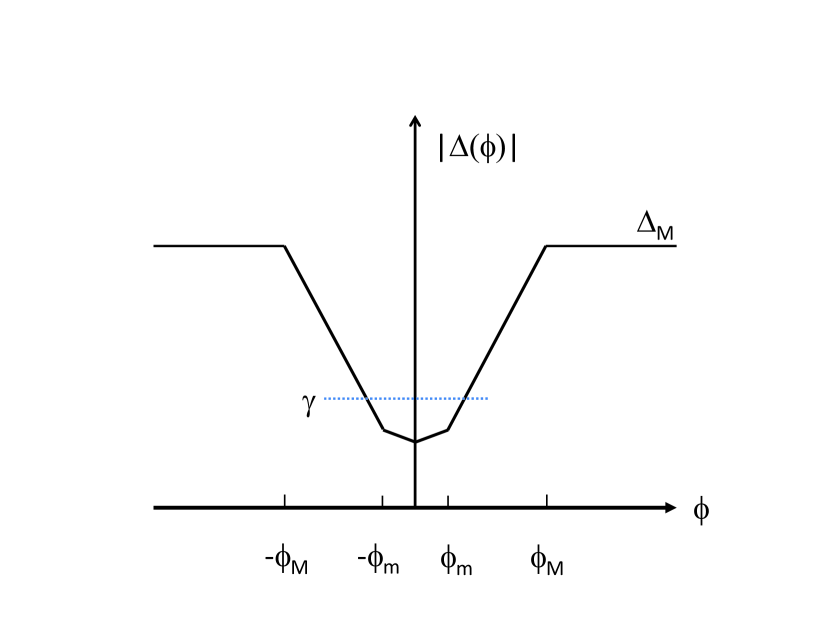
Figure 2: The magnitude of the gap $|\Delta(\phi)|$ near $\phi=0$.

We evaluate the various angular averages that appear in our expressions (34),(35) and (36) for thermo-conductivities. Consider first the quantity in (34). We can rewrite it as

$$\frac{2}{\pi}v_{f}^{2}\int_{0}^{\pi/2}d\phi\frac{\gamma^{2}{\rm cos}^{2}\phi}{\left\{|\Delta(\phi)|^{2}+\gamma^{2}\right\}^{3/2}}$$

and separate the integration into three regions as in (37). For the integral in the first region, we need (we left out the common factor $(2/\pi)v_{f}^{2}$ for simplicity)

$$\int_{0}^{\phi_{m}}d\phi\frac{\gamma^{2}{\rm cos}^{2}\phi}{\left\{|\Delta_{M}|^{2}(\eta_{m}^{2}+\phi^{2})+\gamma^{2}\right\}^{3/2}}$$

If the inequalities concerning $\gamma$ mentioned below (38) holds, we can ignore all terms other than $\gamma$ in the denominator. This contribution is therefore of order $\phi_{m}/\gamma$. The integral for the second contribution can be evaluated. If the above stated inequalities are also satisfied, was stated below (37), we have

$$\int_{\phi_{m}}^{\phi_{M}}d\phi\frac{\gamma^{2}{\rm cos}^{2}\phi}{\left\{|\Delta_{M}|^{2}(\frac{\phi}{\phi_{M}^{2}})^{2}+\gamma^{2}\right\}^{3/2}}\approx\frac{\phi_{M}}{\Delta_{M}}$$ (39)

The third contribution is of order $\gamma^{2}/\Delta_{M}^{3}$. Again using the inequalities stated below (37), the second contribution dominates and we have the approximation

$$\langle v_{fx}^{2}\frac{\gamma^{2}}{D^{3}}\rangle\approx v_{f}^{2}\ \frac{2\phi_{M}}{\pi\Delta_{M}}$$ (40)

We see that we have

$$\frac{K_{xx}^{ns}}{N_{f}v_{f}^{2}\frac{\pi^{2}}{3}T}\approx\frac{2\phi_{M}}{\pi\Delta_{M}}\ ,$$ (41)

the universal value in [2] but in slightly different notations. Thus this model of the gap is consistent with the experimental observations [9, 10], even though the (near) nodes here are not produced by the sign change of the order parameter (as in the case of e.g. $d_{x^{2}-y^{2}}$ in [2]).

Now we turn to $K_{yx}=K_{yx}^{V}$, our main interest in this paper. (For $K_{xx}^{V}$, see A.) Eliminating $\Gamma_{u}$ in favor of $\tilde{\gamma}$ and ${\rm cot}\delta$, we obtain

$$\frac{K_{yx}^{V}}{N_{f}\frac{\pi^{2}}{3}T}=+\frac{\gamma^{3}}{\rm Det}\left(\frac{2{\rm cot}\delta}{\tilde{\gamma}^{2}+{\rm cot}^{2}\delta}\right)\Lambda_{x}\Lambda_{y}$$ (42)

with

$${\rm Det}=1+2\ \frac{\gamma}{\tilde{\gamma}}\ \frac{{\tilde{\gamma}^{2}}-{\rm cot}^{2}\delta}{{\tilde{\gamma}^{2}}+{\rm cot}^{2}\delta}\langle\frac{\Delta_{x}^{2}}{D^{3}}\rangle+\frac{\gamma^{2}}{\tilde{\gamma}^{2}}\langle\frac{\Delta_{x}^{2}}{D^{3}}\rangle^{2}$$ (43)

The required angular averages can be obtained in a similar manner as just described for (34). We have

$$\Lambda_{x}\approx\frac{2v_{f}}{\pi}\frac{\phi_{M}}{\gamma\Delta_{M}}$$ (44)

with the correction term of order $1/\Delta_{M}^{2}$, $\Lambda_{x}=\Lambda_{y}$ by symmetry, and

$$\langle\frac{\Delta_{x}^{2}}{D^{3}}\rangle\approx\frac{2\phi_{M}}{\pi\Delta_{M}}\ln\frac{2\Delta_{M}}{\gamma}+\frac{1-\frac{2\phi_{M}}{\pi/2}}{2\Delta_{M}}$$ (45)

$$\tilde{\gamma}\approx\frac{4\gamma}{\pi}\left(\frac{\phi_{M}}{\Delta_{M}}\ln\frac{2\Delta_{M}}{\gamma}+\frac{\pi/4-\phi_{M}}{\Delta_{M}}\right)$$ (46)

In the above two expressions, the second terms are only logarithmically smaller than the first.

With the above approximations, one can check that the quantity ${\rm Det}$ defined in (29) is only weakly dependent on the phase shift $\delta$. Keeping only the dominant terms in (45) and (46) and using (9) we see that ${\rm Det}\approx 9/4$ near resonance and ${\rm Det}\approx 1/4$ in the Born limit. Suppressing this factor, we get

$$K_{yx}/K_{xx}^{ns}\approx\frac{2\phi_{M}}{\pi}\frac{\gamma}{\Delta_{M}}\ \frac{2{\rm cot}\delta}{{\rm cot}^{2}\delta+(\frac{4\phi_{M}}{\pi}\frac{\gamma}{\Delta_{M}}\ln\frac{2\Delta_{M}}{\gamma})^{2}}$$ (47)

The last fraction is small in both the Born and resonance limit, a result already known in [17]. If however $|{\rm cot}\delta|\sim\tilde{\gamma}$ ($\approx\frac{4\phi_{M}}{\pi}\frac{\gamma}{\Delta_{M}}\ln\frac{2\Delta_{M}}{\gamma}$), we have instead $|K^{yx}/K_{xx}^{ns}|\approx 1/(2\ln\frac{2\Delta_{M}}{\gamma})$, hence the off-diagonal term is only logarithmically smaller than the universal diagonal term.

The value of $\gamma$ depends on the impurity concentration etc. As a reference, [9] estimates that for their samples measured there, $\gamma$ ranges from $~{}0.2K$ to $~{}0.6K$ (while still observing thermal conductance close to the universal value). Estimating $2\Delta_{M}$ by say $5T_{c}$, this logarithmic factor is only roughly $0.13$ and $0.2$ for these $\gamma$’s.

Let us further examine the magnitude of $K_{yx}$. Using the expression for $K_{xx}^{ns}$, and say ${\rm cot}\delta$ is at the above optimal value, we have the following estimate:

$$\frac{K_{yx}}{T}\sim\frac{K_{xx}^{ns}}{2T\ln\frac{2\Delta_{M}}{\gamma}}\sim\frac{\pi^{2}}{6}k_{B}^{2}\frac{N_{f}v_{f}^{2}\ \frac{2\phi_{M}}{\pi\Delta_{M}}}{\ln\frac{2\Delta_{M}}{\gamma}}$$ (48)

In the last expression, we have restored the Boltzmann constant $k_{B}$. Since $N_{f}v_{f}^{2}/\Delta_{M}\sim k_{f}v_{f}/\Delta_{M}\sim E_{f}/T_{c}$ where $E_{f}$ is the Fermi temperature and $T_{c}$ the superconducting critical temperature, we see that the numerator in (48) is large. (For SrRu₂O₄, this ratio is probably of order $10^{2}$).

Hence, unless the phase shift $\delta$ is very close to multiple of $\pi/2$, our computed thermal Hall conductivity is large compared with $k_{B}^{2}T$. Recently, in the context of topological superconductivity, the contribution of edge states to the thermal Hall conductivity is also much discussed [15] (see also e.g., [20, 21, 22, 23]). Assuming the bulk of a chiral superconductor is gapped, the topological edge states become the sole carriers for the heat current. See Fig 3. Consider a sample where say the left is hotter than the right, a net thermal current is then generated in the direction perpendicular to the temperature gradient (upwards along $\hat{y}$ in Fig 3) This thermal Hall conductivity is of order $k_{B}^{2}T$. While this claim is probably correct, we note that the observation of this thermal Hall conductivity is very restrictive. If an impurity band forms (which seems the case for all Sr₂RuO₄ samples studied so far), then the scenario of the present paper applies, giving rise to a much larger thermal Hall conductivity, though the thermal Hall angle would be much smaller since now $K_{xx}$ is finite. (see also B.)

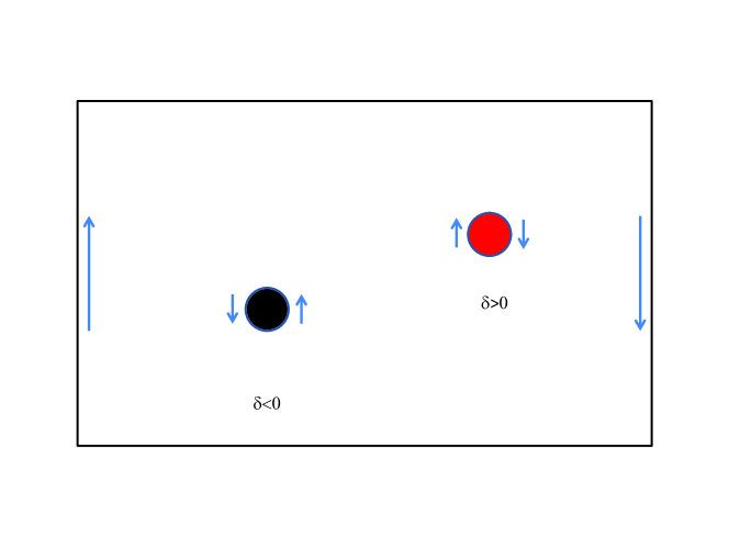
Figure 3: Edge states of a chiral $p_{x}+ip_{y}$ superconductor, with $x$ axis horizontal and $z$ axis pointing out of the paper. Bound states at the left edge of the sample disperse upwards (along $+\hat{y}$) and vice versa at the right edge (see, e.g. [24], note particle current on the left would rather be expected to be downwards along $-\hat{y}$). Also shown are the edge states near a region with repulsive (labeled by $\delta<0$) and attractive (labeled by $\delta>0$) potential inside the sample.

Let us now discuss the sign of this thermal Hall conductivity. Our results shows that the sign of $K_{yx}$ is the same as ${\rm cot}\delta$. (e.g., $K_{yx}>0$ ($K_{xy}=-K_{yx}<0$) if $0<\delta<\pi/2$). It seems that this sign of the thermal Hall conductivity can be understood in the same manner as the edge state contributions [20, 21] mentioned above. Consider extended impurities (rather than point impurities in our calculations) within the sample. A repulsive potential inside the sample has edge states propagating down ($-\hat{y}$) on its left but up on its right. The opposite situation applies if the potential is attractive. If the sample is hotter on the left and cooler on the right ($-(dT/dx)>0$), the edge states near the attractive (repulsive) potential wells would generates a net heat current along $+\hat{y}$ ($-\hat{y}$), if we have many such potential wells (barriers) such that these bounds states overlap so that the heat can propagate through the sample. Now for point impurities with attractive (repulsive) potentials, $\delta>(<)0$ [25]. (More precisely our argument is restricted to $0<\delta<\pi/2$ for attractive potentials and $-\pi/2<\delta<0$ for repulsive potentials. Note however if say $\pi/2<\delta<\pi$, scattering behavior of particles by the attractive potential is as if the scattering were from a repulsive potential with $-\pi/2<\delta<0$.) We thus see that the sign of the thermal Hall conductivities we obtained are of the same sign as what we have if the potentials are extended.

Arfi et al discussed the state $\hat{z}(p_{x}+ip_{y})$. In their plots, they give $K_{xy}>0$ with phase shifts $0<\delta<\pi/2$, thus with a sign opposite to the present results. The author has not yet been able to resolve this discrepancy.

3 Summary and Discussion

In this paper, we have evaluated the $T\to 0$ thermal Hall conductivity for a chiral superconductor where there are momentum directions with strong gap suppression, assuming simple isotropic impurities. We find that the value of this thermal Hall conductivity can be a significant fraction of the diagonal universal component. Detection of this thermal Hall conductivity in Sr₂RuO₄ would be a strong proof that the superconductor possesses a chiral p-wave order parameter. This experimental measurement can however be quite challenging, as it would require a sample with a single domain order parameter. At this moment, there are quite some uncertainties about the domain sizes [26, 27, 28] in this superconductor, but measurement techniques applicable to small system sizes would definitely help here.

We have only considered isotropic impurities, and have ignored possible anisotropic scattering by the impurities, spin-orbit couplings both for the bulk and the impurity scattering. It is entirely feasible that these would also generate a finite thermal Hall conductivity, provided the superconducting order parameter breaks time-reversal and inversion symmetry. The investigation of these possibilities however must be left for the future.

Appendix A Vertex Corrections $K_{xx}^{V}$

Though not directly related to the central theme of this paper, we here investigate further the vertex corrections $K_{xx}^{V}$ to the diagonal terms of the thermal conductance, as we do not find much calculations of this in the literature, with the exception of [5] for the $d_{x^{2}-y^{2}}$ superconductor and the specific model of internodal scattering. The needed expression is already given in (35). For simplicity we shall confine ourselves only to the Born and resonance limits. Again eliminating $\Gamma_{u}$ in favor of $\tilde{\gamma}$ and ${\rm cot}\delta$, and setting $\delta\to 0$, we get (using ${\rm Det}\to 1/4$, note that in this limit, the second and third terms in (27) dominates)

$$\frac{K_{xx}^{V}}{N_{f}\frac{\pi^{2}}{3}T}\approx\frac{4\gamma^{3}}{\tilde{\gamma}^{2}}\left((\tilde{\gamma}-\gamma\langle\frac{\Delta_{x}^{2}}{D^{3}}\rangle\right)\Lambda_{x}^{2}$$ (49)

We see that this is positive definite, that is, the thermal conductivity becomes larger than the universal value when this vertex correction is included. Using the approximate formulas (45) and (46) we get

$$K_{xx}^{V}/K_{xx}^{ns}\approx 1/\ln(2\Delta_{M}/\gamma)$$ (50)

On the other hand, in the resonance limit, we get instead

$$\frac{K_{xx}^{V}}{N_{f}\frac{\pi^{2}}{3}T}\approx-\frac{4\gamma^{3}}{9\tilde{\gamma}^{2}}\left(\tilde{\gamma}+\gamma\langle\frac{\Delta_{x}^{2}}{D^{3}}\rangle\right)\Lambda_{x}^{2}$$ (51)

This is then negative. Using the approximate values discussed before we get

$$\frac{K_{xx}^{V}}{K_{xx}^{ns}}\approx-1/3\ln(2\Delta_{M}/\gamma)$$ (52)

The above mentioned sign change in vertex corrections do not seem to have been noted before in the literature. Durst and Lee [5], who did investigate the vertex corrections for a model of internodal scattering in $d_{x^{2}-y^{2}}$ superconductor, did not mention such possibility of sign change. It is difficult to compare our calculations with [5] since the model are quite different. However, we do note here that the coefficients defined in their (3.17a) and (3.17b) entering their expression for the vertex correction (4.25) for thermal conductivity also consist of two terms appearing as differences, so a sign change may not be out of the question.

Appendix B Other models of the gap

B.1 more general forms of $\eta_{x,y}$

For definiteness, in the text we have introduced a specific model for the functions $\eta_{x,y}$ to introduce near-line nodes in the gap. We shall now argue that many of our results are basically unchanged for other forms of $\eta_{x,y}$ so long as we still have near-line nodes, provide some rather weak conditions remain satisfied. Thus the results given in the text are quite general.

For example, our results are directly applicable to the case where $\eta_{x}$ in Fig 2 in the region $\phi_{m}<\phi<\phi_{M}$ is not directly proportional to $\phi$ but rather have a form say $(1-\phi_{M}/\phi^{\prime}_{M})+\phi/\phi^{\prime}_{M}$, which is still linear in $\phi$ but extrapolate rather to a finite value at $\phi=0$. If the angular averages in (40),(44),(45),(46) etc are still dominated by the contributions where the gap is linear in $\phi$, these equations are then essentially unchanged and our estimate for the thermal Hall conductivities remain valid. With the same reasoning, $\Delta_{x}$ and $\Delta_{y}$ can have additional sign changes as functions of $\phi$ so long as the above mentioned integrals are dominated by the linear regions, in particular $\Delta(\phi)\equiv\Delta_{x}+i\Delta_{y}$ as a function of $\phi$ can have winding number larger than $1$, so long as the angular average (44), which involves $\sim\langle\frac{v_{x}\Delta_{x}}{(\tilde{\gamma}^{2}+|\Delta|^{2})^{3/2}}\rangle$ is non-zero. (For example, if $\Delta_{x}={\rm cos}(3\phi)$ and $\Delta_{y}={\rm sin}(3\phi)$, then the vertex corrections would vanish for isotropic Fermi surface and so $K_{yx}$ would become zero. However, for more general forms of $\Delta(\phi)$ so that $d\Delta(\phi)/d\phi$ or the magnitude $|\Delta(\phi)|$ is not a constant in $\phi$, (44) is in general finite even if $\Delta(\phi)$ still has winding number $3$ or other odd numbers).

Our calculations are valid also for the near nodes are located along $\hat{k}=\pm\hat{x}^{\prime}$ and $\pm\hat{y}^{\prime}$ where $\hat{x}^{\prime}=(\hat{x}+\hat{y})/\sqrt{2}$ and $\hat{y}^{\prime}=(\hat{y}-\hat{x})/\sqrt{2}$. This is because we are only evaluating linear response and we could have use coordinates $\hat{x}^{\prime}$ and $\hat{y}^{\prime}$ for our calculations in text. Tetragonal symmetry implies that $K_{x^{\prime}x^{\prime}}=K_{xx}$ and $K_{y^{\prime}x^{\prime}}=K_{yx}$ etc. Hence our estimates for the thermal conductance should also be applicable for the models in e.g. [14, 15].

B.2 the fully gapped case

Though not the main concern of the present paper, we discuss here also the $T\to 0$ thermal conductance for a two-dimensional chiral superconductor with full isotropic gap, with $\Delta_{x}=\Delta_{M}\cos\phi$ and $\Delta_{y}=\Delta_{M}\sin\phi$. The required angular averages are trivial in the $\gamma\ll\Delta_{M}$ limit. We have

$$\langle v_{fx}^{2}\frac{\gamma^{2}}{D^{3}}\rangle\approx v_{f}^{2}\ \frac{\gamma^{2}}{2\Delta_{M}^{3}}$$ (B.1)

Hence

$$\frac{K_{xx}^{ns}}{N_{f}v_{f}^{2}\frac{\pi^{2}}{3}T}\approx\frac{\gamma^{2}}{2\Delta_{M}^{3}},$$ (B.2)

which is no longer universal, and is smaller than the text for the case of a nodal or near-nodal superconductor by a factor of $~{}(\gamma/\Delta_{M})^{2}$. Furthermore,

$$\tilde{\gamma}\approx\gamma/\Delta_{M}\ ,$$ (B.3)

$$\Lambda_{x}=\Lambda_{y}\approx\frac{v_{f}}{2\Delta_{M}^{2}}$$ (B.4)

and

$$\langle\frac{\Delta_{x}^{2}}{D^{3}}\rangle\approx\frac{1}{2\Delta_{M}}$$ (B.5)

We can verify that ${\rm Det}$ defined in (29) is again $~{}1/4$ and $~{}9/4$ in the Born and resonant limit respectively. Suppressing again this numerical constant, we obtain

$$\frac{K_{yx}}{N_{f}v_{f}^{2}\frac{\pi^{2}}{3}T}\approx\frac{2{\rm cot}\delta}{{\rm cot}^{2}\delta+\frac{\gamma^{2}}{\Delta_{M}^{2}}}\frac{\gamma^{3}}{\Delta_{M}^{4}}$$ (B.6)

If $\rm cot\delta\sim\gamma/\Delta_{M}$, then it turns out that $K^{yx}\sim K_{xx}^{ns}$. Similarly, one can verify that $K_{xx}^{V}$ becomes the same order as $K_{xx}^{ns}$.

References

References

- [1] Lee P A, Phys. Rev. Lett.71, 1887 (1993)
- [2] Graf M J, Yip S-K, Sauls J A and Rainer D, Phys. Rev.B 53, 15147 (1996)
- [3] Graf M J, Yip S-K and Sauls J A, Phys. Rev.B 62, 14393 (2000)
- [4] Shakeripour H, Petrovic C and Taillefer L, New J. Phys.11, 055065 (2009)
- [5] Durst A C and Lee P A, Phys. Rev.B 62, 1270 (2000)
- [6] Maeno Y, Kittaka S, Nomura T, Yonezawa S and Ishida K, J. Phys. Soc. Japan, 81, 01109 (2012)
- [7] Nishizaki S, Maeno Y and Mao Z, J. Phys. Soc. Japan69, 572 (2000)
- [8] Deguchi K, Mao Z Q, Yaguchi H and Maeno Y, Phys. Rev. Lett.92, 047002 (2004)
- [9] Suzuki M, Tanatar M A, Kikugawa N, Mao Z Q, Maeno Y and Ishiguro T, Phys. Rev. Lett.88, 227004 (2002)
- [10] Suderow H, Brison J P, Flouquet J, Tylar A W, Maeno Y, J. Phys.: Condens. Matter10, L597 (1998)
- [11] Graf M and Balatsky A V, Phys. Rev.B 62, 9697 (2000)
- [12] Nomura T and Yamada K, J. Phys. Soc. Japan71, 404 (2002)
- [13] Yanase Y, Jujo T, Nomura T, Ikeda H, Hotta T and Yamada Y, Phys. Rep. 387, 1 (2003)
- [14] Wang Q H, Platt C, Yang Y, Honerkamp C, Zhang F C, Hanke W, Rice T M and Thomale R, EPL, 104, 17103 (2013)
- [15] Scaffidi T and Simon S H, Phys. Rev. Lett.115, 087003 (2015)
- [16] Yip S and Sauls J A, J Low Temp. Phys. 86, 257 (1992)
- [17] Arfi B, Bahlouli H and Pethick C J, Phys. Rev.B 39, 8959 (1989)
- [18] Raghu S, Kapitulnik A and Kivelson S A, Phys. Rev. Lett.105 136401 (2010)
- [19] Xu D, Yip S K and Sauls J A, Phys. Rev.B 51, 16233 (1995)
- [20] Read N and D Green, Phys. Rev.B 61, 10267 (2000)
- [21] Senthil T, Marston J B and Fisher M P A, Phys. Rev.B 60, 4245 (1999)
- [22] Nomura, Ryu S, Furusaki A and Nagaosa N, Phys. Rev. Lett.108, 026802 (2012)
- [23] Sumiyoshi H and Fujimoto S, J. Phys. Soc. Japan82, 023602 (2013)
- [24] Stone M B, Phys. Rev.B 69, 184511 (2004)
- [25] Sakurai J J, Modern Quantum Mechanics, Addison-Wesley (1994).
- [26] Kidwingira F, Strand J D, Van Harlingen D J and Maeno Y, Science, 314 (2006)
- [27] Kallin C and Berlinsky A J, J. Phys.: Condens. Matter21, 164210 (2009)
- [28] Hicks C W, Kirtley J R, Lippman T M, Koshnick N C, Huber M E, Maeno Y, Yuhasz W M, Maple M B and Moler K A, Phys. Rev.B 81, 214501 (2010)