Stitching Stabilizer:
Two-frame-stitching Video Stabilization for Embedded Systems

Abstract

In conventional electronic video stabilization, the stabilized frame is obtained by cropping the input frame to cancel camera shake. While a small cropping size results in strong stabilization, it does not provide us satisfactory results from the viewpoint of image quality, because it narrows the angle of view. By fusing several frames, we can effectively expand the area of input frames, and achieve strong stabilization even with a large cropping size. Several methods for doing so have been studied. However, their computational costs are too high for embedded systems such as smartphones.

We propose a simple, yet surprisingly effective algorithm, called the stitching stabilizer. It stitches only two frames together with a minimal computational cost. It can achieve real-time processes in embedded systems, for Full HD and 30 FPS videos. To clearly show the effect, we apply it to hyperlapse. Using several clips, we show it produces more strongly stabilized and natural results than the existing solutions from Microsoft and Instagram.

I Introduction

Smartphones have recently become very popular worldwide. For consumers, one of the criteria for choosing a handset is the camera features. Although the capability of taking beautiful photos is an important factor, the video quality should not be overlooked. There are many features that affect the overall video quality of smartphones such as auto focus, auto exposure and auto white balance. One important feature is stabilization.

Three are major video stabilization mechanisms, namely mechanical image stabilization, optical image stabilization (OIS), and electronic image stabilization (EIS). EIS is a practical solution for embedded systems such as smartphones, because it is inexpensive and requires no special hardware such as gyroscope sensors or optical systems. The simplest algorithm for EIS creates output frames by cropping the input in a way that cancels camera shake. One advantage of this algorithm is its simplicity. Only limited resources are available for embedded systems, so simplicity is crucial to achieve real-time processes such as video stabilization. Moreover, this is a GPU friendly algorithm, which has become an important factor in recent technology trends. Cropping, or geometrical transformation, of image frames is a strong point of the GPU.

EIS does have a weak point, however. That is, it sacrifices the angle of view (AOV) of the camera, which is important for quality. This is an inevitable consequence of cropping. Less cropping is advantageous for stabilization but disadvantageous for the AOV. Hence, we must tune and find the best balance for the cropping size.

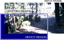
Let us consider an EIS system with a large cropping size. Although the AOV is wide in that case, there is no room to absorb camera shake. If we want stabilized results even in this situation, it is necessary to accept cropping outside the input frame. As there are no defined pixels outside the frame, the result must contain undefined or deficit regions as depicted in Figure 1 (a). If there was a method to fill in this deficit, we could obtain the stabilized result with a wide AOV. The filling process corresponds to effectively expanding the area of input frames, and several techniques have been developed that try to achieve this.

(a) No-stitching stabilizer.

(b) Stitching stabilizer.

(c) Stitching example.

Figure 1: (a) When we try to stabilize a large degree of camera shake with a large cropping size, there is a deficit region. This is because there are no defined pixels outside the frame. To achieve strong stabilization with a large cropping size, or a wide angle of view, we need to find some ways to fill in this deficit. (b) In our approach, the stitching stabilizer, the current and previous frames are stitched together along the seam to effectively expands the area of input frames. This fills the deficit in and strong stabilization with a wide angle of view is achieved. The algorithm searches for the seam so that stitching becomes as unnoticeable as possible. In this example, the seam should avoid the face of a person. (c) In the left panel, the undefined region is simply filled by the previous frame and the face is cut in half. The right panel is our stitching result. The seam avoids the face and the result is more natural.

Litvin et al. Litvin et al. (2003) employed mosaicing from several adjacent frames to fill in the deficit. The filling process is done by averaging corresponding valid pixels. Their method does not consider non-planar or moving objects, though, so Matsushita et al. Matsushita et al. (2006) and Chen et al. Chen et al. (2008) proposed methods that compensate for local motion in addition to global or planar motion. All three algorithms require several (more than two) input frames to generate one output and perform complicated calculations for every frame. Hence, they are not applicable for embedded system because of the high computational cost.

Although the goal is different, the hyperlapse algorithm proposed by Kopf et al. Kopf et al. (2014) shows a similar effect. Hyperlapse is a kind of time-lapse video that is captured during motion such as while walking or driving a car. This has become a trend for mobile video, and some apps (http://research.microsoft.com/en-us/um/redmond/projects/hyperlapseapps/; https://hyperlapse.instagram.com/) for it have been released in recent years. They reconstruct a 3D world from video input and virtually re-capture hyperlapse videos in their 3D world. Although this solves the AOV problem and the results are impressive, it also has a high computational cost and thus cannot be applied to embedded systems.

I.1 Our approach

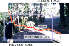
In this approach, we basically follow the same idea, namely filling in the deficit, with an algorithm that is fast enough for embedded systems. To achieve the fast process, we use only two frames for filling. Under this limited condition, we cannot use methods applied in previous studies Litvin et al. (2003); Matsushita et al. (2006); Chen et al. (2008). Therefore, we take a new approach, stitching stabilizer, in which the two frames are simply stitched together along an unnoticeable seam. This is shown in Figure 1 (b). The stitching process effectively expands the area of input frames, and the deficit regions can be filled in. This paper shows that stitching only two frames with a simple algorithm can improve stabilization quality remarkably.

There are two ways to stitch. One is to stitch the current and previous frames, and the other is to stitch the current and the next (subsequent) frames. Both possibilities are considered in the following discussions. Then, the $(n+1)$-th frame is required to make the $n$-th result and this introduces a latency of one frame. This is a drawback, although it is outweighed by the positive effect.

To clearly show its effect, we applied the stitching stabilizer to hyperlapse videos. In hyperlapse, camera shake is effectively increased because of fast-forwarding. Therefore, in the conventional stabilizer, a small cropping region, or a narrow AOV, is unavoidable to achieve strong stabilization. Here, conventional refers to the stabilizer without stitching. We show that the stitching stabilizer remarkably reduced camera shake compared to the conventional stabilizer, without losing the AOV. Moreover, it produced a more stabilized and natural output than existing real-time hyperlapse methods Karpenko (2014); Joshi et al. (2015).

This paper is organized as follows. Related work is summarized in section II. In section III, we explain the algorithm of the video stabilizer without stitching, and the extension of it to the stitching stabilizer is given in section IV. We apply the stitching stabilizer to hyperlapse in section V, and the results of applying our algorithm are explained and discussed in section VI. Section VII is the conclusion.

II Related work

In this section, we summarize related work on video stabilization, hyperlapse, video completion and image stitching.

II.1 Video stabilization

There are 2D and 3D models of video stabilization algorithms. Although the structure-from-motion based 3D model is more powerful Liu et al. (2009), it consumes large computational resources and is not robust. The 2D model Litvin et al. (2003); Matsushita et al. (2006); Grundmann et al. (2011) uses 2D geometric transformation, such as affine or perspective transformation, to describe its global motion. Hence, it is fast and robust because of its simplicity and is popular in embedded systems. Some methods lie in between the 2D and 3D models Liu et al. (2011); Goldstein and Fattal (2012); Liu et al. (2013). In addition, an algorithm that utilizes a hardware gyroscope has also been studied Karpenko et al. (2011).

Another important factor affecting video stabilization is rolling shutter (RS) distortion. This distortion is related to the physical motion of the camera. Hence, there are many algorithms for removing RS distortion by modeling motion: translational motion along $x$ and $y$ axes Im et al. (2006), affine transformation Cho and Hong (2007), row-by-row motion Liang et al. (2008); Baker et al. (2010), and 3D motion Forssén and Ringaby (2010). These motion based methods require hardware-dependent parameters to remove distortion, but algorithms that do not require prior knowledge have also been developed Grundmann et al. (2012); Liu et al. (2013).

We prefer robustness as a solution for embedded systems. For many casual users, there are no retakes. It is therefore much more important to produce a robust result with acceptable quality than a perfect but not very robust one. Therefore, we use 2D stabilization with perspective transformation. Of course, affine transformation is more robust, but its quality is unsatisfactory. For the same reason, we use the translational model for RS distortion Im et al. (2006). In this case, the distortion can be written as a matrix and is easy to implement.

II.2 Hyperlapse

For hyperlapse, as stated, the algorithm of Kopf et al. Kopf et al. (2014) achieves impressive results, but its computational cost is too high for our purposes. Real-time algorithms have been studied by Karpenko Karpenko (2014) for Instagram’s app and Joshi et al. Joshi et al. (2015) for Microsoft’s mobile app.

Karpenko’s approach is fairly straightforward. The algorithm combines the hardware gyroscope and image frames to calculate 2D global motion and stabilizes it. To create hyperlapse, the input frame is skipped according to a user set parameter, for example $\times 4$ or $\times 8$. The algorithm by Joshi et al. is a bit tricky. The global motion detection is purely software-based conventional 2D detection. However, they select the input frames to achieve smoother results. In other words, they do not skip frames with even spacing. By selecting frames, they can avoid very shaky frames and achieve strong stabilization. Poleg et al. created another frame selection algorithm Poleg et al. (2015). However, its computational cost is also too high to be implemented in embedded systems.

Our approach is between Kopf et al. and Karpenko. It is fast and based on the conventional framework, while it utilizes several (in our case two) input frames to produce output. Although the frame selection is compatible with the stitching stabilizer, we employ frame skipping with even spacing, as a start.

II.3 Video completion and image stitching

We have investigated various methods for filling in deficit regions. One such method is video completion Wexler et al. (2004); Jia et al. (2004); Patwardhan et al. (2007), which is a technique to fill in missing parts of videos. It has already been studied in the context of video stabilization Litvin et al. (2003); Matsushita et al. (2006); Chen et al. (2008). The problem with these methods is that they are computationally expensive for our purpose. Therefore, we used the second candidate, simple stitching of two adjacent frames, in the stitching stabilizer.

Image stitching is a very common process in computer vision Davis (1998); Efros and Freeman (2001); Kwatra et al. (2003); Gu et al. (2009). The problem we have been focusing on is finding the optimal seam. In that sense, seam carving Avidan and Shamir (2007) and digital photomontage Agarwala et al. (2004) are somewhat related.

There are several popular seam finding algorithms, including Dijkstra’s algorithm Dijkstra (1959); Davis (1998); Avidan and Shamir (2007), dynamic programming (DP) Efros and Freeman (2001); Gu et al. (2009), and graph cuts Kwatra et al. (2003); Agarwala et al. (2004).

We used Dijkstra’s algorithm for the stitching stabilizer, and the discussion of this is in subsection IV.1.

III Conventional video stabilizer

We explain our algorithm of the conventional stabilizer. We consider stabilization with 2D perspective transformation.

As a motion detection algorithm, we use the pyramid image approach Bergen et al. (1992). The process at each layer is a little different from the standard one. First, we track sparsely selected Harris-Stephens feature points Harris and Stephens (1988) independently by block matching which minimizes the sum of absolute difference. The initial vectors for each block matching process are determined by the transformation of the lower layer. Second, we calculate the perspective transformation of this layer by the least squares method.

Our algorithm for EIS is indicated as ALGORITHM 1. CalcMotion is a function that calculates the perspective transformation $M$ between two adjacent frames:

$$(x_{\text{curr}},y_{\text{curr}},1)^{\rm T}\sim M(x_{\text{prev}},y_{\text{prev}},1)^{\rm T},$$ (1)

where $(x_{\text{curr}},y_{\text{curr}},1)$ and $(x_{\text{prev}},y_{\text{prev}},1)$ are corresponding coordinates in the current and previous frames. Based on this $M$ and the previous results, Filter determines the perspective matrix $P$ for cropping. Crop is a function to perform cropping based on $P$. EnsureInside requires more explanation than the other functions. In our framework, Filter itself does not ensure that the cropping region is inside the frame. Hence, we need another function, in this case EnsureInside, to do this. CalcCroppingBoundary calculates the boundary region of the cropping. While the cropping region is not inside the frame, the matrix $P$ is repeatedly blended with the identity matrix. This blending corresponds to bringing the matrix to near the identity. The constant $\varepsilon$ is the blending coefficient and we set $\varepsilon=0.01$. EnsureInside adds unfiltered motion to the output. Hence, when IsInside frequently returns false, the output video becomes shaky.

List of Algorithms 1 Algorithm for EIS.

1:$P\leftarrow identity$

2:while there is a frame to be processed do

3:     Load the next input frame

4:     $M\leftarrow$ CalcMotion(from previous to current)

5:     $P\leftarrow$ Filter($M,P$)

6:     $P\leftarrow$ EnsureInside($P$)

7:     Crop($P$)

8:end while

9:

10:function EnsureInside($P$)

11:     $crop\leftarrow$ CalcCroppingBoundary($P$)

12:     while IsInside($crop$) is false do

13:         $P\leftarrow$ToIdentity($P,\varepsilon$)

14:         $crop\leftarrow$ CalcCroppingBoundary($P$)

15:     end while

16:     return $P$

17:end function

18:

19:function ToIdentity($P,\varepsilon$)

20:     $I\leftarrow identity$

21:     Return $\varepsilon I+(1-\varepsilon)P$

22:end function

23:

24:function IsInside($crop$)

25:     if $crop$ is inside the input frame then

26:         return true

27:     else

28:         return false

29:     end if

30:end function

 

In this stabilization framework, the most important factor is how the function Filter works.

III.1 Rolling shutter distortion

Before explaining the Filter algorithm, we summarize how we treat RS distortion. In a digital camera, RS distortion is a problem unique to CMOS sensors without a mechanical shutter, and CCD sensors are RS distortion-free. Because CMOS sensors have recently become very popular in smartphones and digital still cameras, this distortion needs to be addressed. Moreover, the algorithm developed for CMOS sensors is also effective for CCD sensors, but not vice versa.

Let us define the coordinates on the distorted input frame as $(x,y,1)$ and that on the ideal distortion-free frame as $(X,Y,1)$. There must be a relationship between them, such as $(x,y,1)^{\rm T}={\cal D}((X,Y,1)^{\rm T})$. In general, this function ${\cal D}$ cannot be written in a matrix form. However, when the global motion between adjacent frames is just a translation along the $x$ and $y$ axes with constant velocity Im et al. (2006):

$$M=\begin{pmatrix}1&0&t_{x}\\ 0&1&t_{y}\\ 0&0&1\end{pmatrix},$$ (2)

${\cal D}$ can be written as a matrix:

$$D=\begin{pmatrix}1&-t_{x}/H&0\\ 0&1-t_{y}/H&0\\ 0&0&1\end{pmatrix}^{-1},$$ (3)

where $H$ is an effective height for the sensor and is equal to or larger than the actual height. $H$ takes a large value for a fast scanning sensor and a small value for a slow sensor. In realistic scenes, $M$ is not a purely translational matrix. It is composed of eight variables:

$$M=\begin{pmatrix}a&b&c\\ d&e&f\\ g&h&1\end{pmatrix},$$ (4)

where we set the right-bottom component to one, because the overall factor is meaningless. For the video, the most dominant part of the matrix $M$ might be the translations $c$ and $f$. Therefore, the following approximation seems to be a practical one:

$$D=\begin{pmatrix}1&-c/H&0\\ 0&1-f/H&0\\ 0&0&1\end{pmatrix}^{-1},$$ (5)

where we assume that RS distortion is caused only by the translational components of $M$. Using this matrix, we can obtain the correspondence between the distorted and distortion-free coordinates: $(x,y,1)^{\rm T}\sim D(X,Y,1)^{\rm T}$. Note that the symbol “$\sim$” denotes that the right-hand side and the left-hand side are equal up to an overall factor.

III.2 Filter design

Here, we show how the function Filter works in our stabilizer. Let us define the matrix $M_{n}$ that relates the $(n-1)$-th input frame coordinates $(x_{n-1},y_{n-1},1)$ and the $n$-th input frame coordinates $(x_{n},y_{n},1)$:

$$(x_{n},y_{n},1)^{\rm T} \sim M_{n}(x_{n-1},y_{n-1},1)^{\rm T}$$

$$\sim D_{n}N_{n}D_{n-1}^{-1}(x_{n-1},y_{n-1},1)^{\rm T}.$$ (6)

This can be obtained by the function CalcMotion in ALGORITHM 1. We separate the RS distortion matrix $D_{n}$ and $D_{n-1}$ and get the distortion-free matrix $N_{n}\equiv D_{n}^{-1}M_{n}D_{n-1}$. As we have discussed, our expression for $D_{n}$, equation (5), is an approximated one, so $N_{n}$ is not exactly distortion-free. Even so, it is still more manageable than $M_{n}$.

To process the $n$-th frame, the result of the $(n-1)$-th frame is already known. It is the 2D perspective matrix $P_{n-1}$ which represents the relation between the coordinates on the $(n-1)$-th output frame $(X_{n-1},Y_{n-1},1)$ and those on the $(n-1)$-th input frame $(x_{n-1},y_{n-1},1)$:

$$(x_{n-1},y_{n-1},1)^{\rm T} \sim P_{n-1}(X_{n-1},Y_{n-1},1)^{\rm T}$$

$$\sim D_{n-1}Q_{n-1}(X_{n-1},Y_{n-1},1)^{\rm T}.$$ (7)

This $P_{n-1}$ determines how the $(n-1)$-th input frame is cropped to create the corresponding output frame. The distortion-free cropping matrix $Q_{n-1}$ is defined as $Q_{n-1}\equiv D_{n-1}^{-1}P_{n-1}$.

The filtering algorithm determines $Q_{n}$ based on $N_{0}...N_{n}$ and $Q_{0}...Q_{n-1}$. Then, because $D_{n}$ is obtained from $M_{n}$, we can get $P_{n}\sim D_{n}Q_{n}$ and perform cropping. We consider two extreme cases for filtering. One is $Q_{n}\sim N_{n}Q_{n-1}$. From the above equations, we get:

$$(x_{n-1},y_{n-1},1)^{\rm T}\sim D_{n-1}Q_{n-1}(X_{n},Y_{n},1)^{\rm T}.$$ (8)

This is the relation between the $n$-th output coordinates and $(n-1)$-th input coordinates. This equation and equation (7) indicate that the output frames are identical for the $(n-1)$-th and $n$-th frames. Therefore, the result must be a video with no motion. This interpretation is based on the unrealistic assumption that all motions are written by the 2D perspective transformation. Even so, it might be true even for actual situations that the stabilizer removes almost every camera motion, including panning or tilting. Another case is $Q_{n}\sim Q_{n-1}$. In this case, the cropping matrix of the $n$-th frame is the same as that of the $(n-1)$-th frame, except for the RS distortion. This means there is no stabilization. Needless to say, both cases are undesirable. What we expect from video stabilization is stabilization for high frequency motion and no stabilization for low frequency motion. In other words, $Q_{n}\sim N_{n}Q_{n-1}$ for high frequency and $Q_{n}\sim Q_{n-1}$ for low frequency. Formally, we can write this as:

$$Q_{n}\sim f(N_{n}^{-1})N_{n}Q_{n-1},$$ (9)

where the function $f$ is a low pass filter. This $f(N_{n}^{-1})$ represents how the camera moves in the output video, because $Q_{n}\sim N_{n}Q_{n-1}$ corresponds to the case without camera motion.

To design the filter for $N_{n}^{-1}$, we first consider the most important elements. In video stabilization, these are the rotational angles. While we follow the conventional yaw-pitch-roll notation, our method is applicable for any of the Euler angles. It is difficult to deduct exact angles from $N_{n}^{-1}$, because it is not exactly distortion-free. Hence, we simply estimate them. For example, even the following rough estimation works:

$$\alpha_{n}=\sin^{-1}\frac{c^{\prime}_{n}}{\ell},\quad\beta_{n}=-\sin^{-1}\frac{f^{\prime}_{n}}{\ell},\quad\gamma_{n}=\tan^{-1}\frac{d^{\prime}_{n}}{e^{\prime}_{n}},$$ (10)

where $\alpha_{n},\beta_{n}$, and $\gamma_{n}$ are the estimated yaw, pitch, and roll angles of $N_{n}^{-1}$, respectively and $\ell$ denotes the focal length of the camera. The variables $c^{\prime}_{n},f^{\prime}_{n},d^{\prime}_{n}$ and $e^{\prime}_{n}$ are the components of the matrix $N_{n}^{-1}$:

$$N_{n}^{-1}=\begin{pmatrix}a^{\prime}_{n}&b^{\prime}_{n}&c^{\prime}_{n}\\ d^{\prime}_{n}&e^{\prime}_{n}&f^{\prime}_{n}\\ g^{\prime}_{n}&h^{\prime}_{n}&1\end{pmatrix}.$$ (11)

Then, we decompose $N_{n}^{-1}$ as follows:

$$N_{n}^{-1} \sim R_{\rm yaw}(\alpha_{n})R_{\rm pitch}(\beta_{n})R_{\rm roll}(\gamma_{n})L_{n},$$ (12)

where $R_{\rm yaw}(\alpha_{n}),R_{\rm pitch}(\beta_{n})$, and $R_{\rm roll}(\gamma_{n})$ are the matrix representation of the estimated yaw, pitch, and roll rotations. The term $L_{n}$ includes all other motions and errors of estimation. In normal cases, this $L_{n}$ is a minor contributor to quality. Therefore, we omit this term in the low pass filter:

$$f(N_{n}^{-1})\sim R_{\rm yaw}(g(\alpha_{n}))R_{\rm pitch}(g(\beta_{n}))R_{\rm roll}(g(\gamma_{n})),$$ (13)

where $g$ is a low pass filter for scalar values. Again, $g(\alpha_{n}),g(\beta_{n})$, and $g(\gamma_{n})$ represent how the camera moves.

For simplicity, we use the same type of filters for $\alpha_{n},\beta_{n}$, and $\gamma_{n}$. There are many possibilities for this filter algorithm. Averaging recent values is a simple example. Instead, we use the mid-range value that is defined as:

$$\text{mid-range value}(array)=\frac{\text{max}(array)+\text{min}(array)}{2},$$ (14)

where the variable $array$ is an array that stores recent input values. The advantage of the mid-range value in comparison to the average value is quick response, which is an important factor for video stabilization. Any input larger than previous values gives a $50\%$ contribution, instantly. The important parameter for this algorithm is the size of $array$, and the typical value is $8$.

There is one last thing that needs to be addressed. Because equation (9) accumulates motion data at each frame, it also accumulates undesirable error motions. The errors can be derived from motion detection, the approximation of RS distortion, and the rough decomposition of $N_{n}^{-1}$. We should suppress this error accumulation. We decompose $Q_{n}$ as in equation (12):

$$Q_{n}\sim R_{\rm yaw}(A_{n})R_{\rm pitch}(B_{n})R_{\rm roll}(\Gamma_{n})\Lambda_{n},$$ (15)

where $A_{n},B_{n}$ and $\Gamma_{n}$ respectively represent yaw, pitch, and roll for the distortion-free cropping matrix. Only the term $\Lambda_{n}$ requires special treatment here. As other terms are yaw-pitch-roll rotations, they can be treated in the low pass filter with a minor change. In the ideal case where every motion is composed of only yaw-pitch-roll rotations, this $\Lambda_{n}$ must coincide with the identity matrix. Hence, to simply suppress the errors, we blend $\Lambda_{n}$ with the identity:

$$\Lambda_{n}\leftarrow(1-\eta)\Lambda_{n}+\eta I,$$ (16)

where $\eta$ is a small constant, and the typical value is 0.25.

IV Stitching stabilizer

We explained the algorithm of the conventional stabilizer. In this section, we extend it to the stitching stabilizer using the same framework, ALGORITHM 1. For simplicity, we rename the current frame as the main frame and the previous or next frame as the sub-frame. As explained in Figure 2, some cropping configurations, that cannot be used in the conventional stabilizer, can be used in the stitching stabilizer. Hence, we should replace the IsInside function of ALGORITHM 1 with new one.

Figure 2: In the conventional stabilizer, the cropping region must be inside the main frame. Hence, there is a deficit region in this cropping configuration, and it cannot be used. In the stitching stabilizer, however, this configuration is deficit-free, because the cropping region is inside the combined boundary of the main and sub-frames. Therefore, the stitching stabilizer can absorb camera shake that the conventional one cannot.

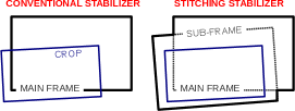
The new algorithm for IsInside is ALGORITHM 2. The sub-frame boundary is aligned with the main frame to obtain the combined boundary, and Trans does this using equation (6). Note that perspective transformation makes a rectangle a quadrangle. Combine combines two quadrangles to return one polygon that corresponds to the combined boundary. If the cropping boundary is inside the current-previous polygon, we can get no deficit output with the current-previous stitching. Therefore, we return true. The same thing can be said for the current-next case.

List of Algorithms 2 IsInside functions for the stitching stabilizer.

1:function IsInside($crop$)

2:     $M\leftarrow$ CalcMotion(from previous to current)

3:     if IsInsideCombined($crop,M$) then

4:         return true $\triangleright$ current-previous stitching

5:     end if

6:

7:     $M\leftarrow$ CalcMotion(from next to current)

8:     if IsInsideCombined($crop,M$) then

9:         return true $\triangleright$ current-next stitching

10:     end if

11:     return false

12:end function

13:

14:function IsInsideCombined($crop,M$)

15:     $main\leftarrow$ Rect($0,0$,input width,input height) $\triangleright$ the main frame boundary

16:     $sub\leftarrow$ Trans($main,M$) $\triangleright$ the sub-frame boundary aligned with the main

17:     $combined=$ Combine($main,sub$) $\triangleright$ the combined valid boundary

18:     if $crop$ is inside $combined$ then

19:         return true

20:     else

21:         return false

22:     end if

23:end function

 

Then, let us consider cropping and stitching. The cropping of the main frame is essentially the same as that of the conventional stabilizer:

$$(x_{n},y_{n},1)^{\rm T}\sim P_{n}(X_{n},Y_{n},1)^{\rm T}.$$ (17)

Some pixels of $(x_{n},y_{n},1)$ are outside the main frame, and the sub-frame fills in this undefined region. For stitching, the sub-frame has to be aligned with the main frame. From equation (6),

$$(x_{n-1},y_{n-1},1)^{\rm T}\sim M_{n}^{-1}P_{n}(X_{n},Y_{n},1)^{\rm T},$$ (18)

$$(x_{n+1},y_{n+1},1)^{\rm T}\sim M_{n+1}P_{n}(X_{n},Y_{n},1)^{\rm T}.$$ (19)

These equations transform the output frame coordinates to the sub-frame coordinates and the alignment can be performed.

As stated, the optimal seam is required for the stitching, and the algorithm for finding it is explained in the next two subsections. After the optimal seam is found, the merging process is straightforward. In the stitching stabilizer, Crop in ALGORITHM 1 also performs seam-finding and merging, in addition to cropping.

IV.1 Optimal seam algorithm

For finding the optimal seam, we categorize each frame with deficit regions into four types, as in Figure 3. We expand the deficit region so that it matches one of these types. This expansion is performed under the condition that the change of the area takes the minimum value. When deficit regions are not connected, we virtually connect these regions and assign them to one of these types, with the minimum expansion.

Figure 3: Four types of expanded deficit regions (hatched area), examples of the corresponding seam (blue lines), and examples of actual deficit regions (blue area). We categorize deficit regions to these four types with the minimum expansion. Each type I, L, and C includes three variations of its $90^{\circ}$, $180^{\circ}$, and $270^{\circ}$ rotations.

Here, we compare three algorithms, namely DP, Dijkstra’s algorithm and, graph cuts. The order of computational complexity of the optimally implemented graph cuts is $O(VE)$ Orlin (2013) and that of Dijkstra’s algorithm is $O(V\log V+E)$ Cormen et al. (2009), where $E$ and $V$ denote the number of edges and nodes, respectively. The complexity of DP used in this kind of problem is $O(V)$ Gu et al. (2009).

The fastest algorithm is desirable when taking our purpose into account. However, DP is one-directional which means that it can only solve certain cases such as those with a top-bottom or left-right seam. According to our categorization, it can only solve type I and is therefore not sufficient. The difference in complexity between DP and graph cuts is huge, so graph cuts is a highly undesirable solution. However, the difference between DP and Dijkstra’s algorithm is not that significant, so they are practically almost the same. The problem with Dijkstra’s algorithm is it can only solve the shortest path problem and cannot solve type O. Type O is empirically rare, though, so we give up type O and use Dijkstra’s algorithm for the stitching stabilizer.

Note that we must change the function IsInside in ALGORITHM 2, because we have given up type O. The change itself is minor: When the deficit is type O, we only need to prevent the function from returning true. The final important factor is that we use $1/4$ shrunken images to accelerate the processing time.

IV.2 Finding the optimal seam

To find the seam with Dijkstra’s algorithm, we must define what the nodes, edges, and costs mean in our case. We explain this using Figure 4. The edges are defined as the borders of image pixels and the nodes are the criss-crossed points of four neighboring pixels. We assign costs only for edges:

$${\rm cost}_{AB} =\left|L_{A}^{\rm main}-L_{B}^{\rm sub}\right|+\left|L_{A}^{\rm sub}-L_{B}^{\rm main}\right|,$$ (20)

where $L_{A}$ and $L_{B}$ denote the luma values for any pair of adjacent pixels, and $cost_{AB}$ is the cost of the edge between them. With this definition, the cost becomes small when there is only a small difference in the luma values across the seam. Hence, the resulting seam might be the most unnoticeable one for stitching. The cost is set to infinity in the vicinity of the deficit region so that the seam does not cross it. On the border of the output frame, the edge cost cannot be determined by the above equations. We set these border costs to zero, except for those inside the deficit region.

Figure 4: In our search with Dijkstra’s algorithm, nodes are the criss-crossed points of pixels and edges are the border lines of pixels. Costs are only assigned to edges.

Then, we set the search region and the start and end points. Using the main frame is generally preferable to using the sub-frame. Hence, the optimal seam should be drawn near the perimeter of the main frame. The simplest way to enforce this is to restrict the search region, which is also beneficial for the processing time. As depicted in Figure 5, we set the search region based on the shape and size of the expanded deficit region. Both ends of the search region are assigned to start or end points.

Figure 5: Expanded deficit region (sparsely hatched region), search region (both densely blue hatched and sparsely hatched regions), and start and end points (circled in red). We set the search region using the type of the expanded deficit region. In our implementation, the width of the search region was set $2-4$ times wider than that of the expanded deficit region.

After setting the costs, the search region and the start and end points, we can apply Dijkstra’s algorithm to find the optimal seam for stitching.

V Hyperlapse

In this section, the extension of the stitching stabilizer to hyperlapse videos is explained. To process hyperlapse in mobile devices, it is possible to perform a preprocess during the video capture. In our case, global motion detection is done as the preprocess. This is because, it is highly advantageous for achieving strong stabilization, to know all global motions of the clip in the main process. During the video capture, the function CalcMotion in ALGORITHM 1 is called every frame, and its result, the motion matrix $M$, is stored as a kind of meta data.

ALGORITHM 3 is the main hyperlapse process. This is similar to the standard stabilization algorithm, ALGORITHM 1. Here, standard means the algorithm explained in sections III and IV. The difference is only in the loop of the image frame and motion data skipping. Here, $skip$ is the number of skipped frames. In the stitching hyperlapse, the sub-frame corresponds to the $skip$-frame previous or next frame. LoadMotion loads the corresponding global motion data that were stored by the preprocess algorithm.

List of Algorithms 3 Main process for hyperlapse.

1:$P\leftarrow identity$

2:while there is a frame to be processed do

3:     $M\leftarrow identity$

4:     for $i\leftarrow 1,skip$ do $\triangleright$ frame skipping

5:         Load the next input frame

6:         $M\leftarrow M\times$ LoadMotion(from previous to current)

7:     end for

8:     $P\leftarrow$ Filter($M,P$)

9:     $P\leftarrow$ EnsureInside($P$)

10:     Crop($P$)

11:end while

 

V.1 Filter design for hyperlapse

Part of the low pass filter should be redesigned so that it matches hyperlapse videos. Specifically, we change filter $g$ in equation (13). The most important difference between standard stabilization and hyperlapse is that we can utilize all global motion data including future data.

We call filtered rotational values in equation (13), namely $g(\alpha_{n}),g(\beta_{n})$, and $g(\gamma_{n})$, camera velocities. We consider that the ideal output for hyperlapse is an output with constant camera velocities. This is difficult to achieve in many realistic cases, however, so we have to accept several turns. In addition, the stabilizer should crop the near-center regions of the input frames, if possible. This is because, the object that users want to capture might be in the center of the frame. Needless to say, a highly undesirable output is what goes outside the input frame, and EnsureInside works to make sure it is inside. In consideration of the conditions above, we try to minimize the following cost to get the filtered values of $\alpha_{n},\beta_{n}$, and $\gamma_{n}$ for each frame:

$${\rm cost} =\varepsilon_{t}\times\text{number of turns}$$

$$+\sum_{i\in\text{all frames}}\left(\varepsilon_{\alpha}{\rm abs}(A_{i})+\varepsilon_{\beta}{\rm abs}(B_{i})+\varepsilon_{\gamma}{\rm abs}(\Gamma_{i})\right)$$

$$+\varepsilon_{p}\times\text{number of attempts}$$

$$\qquad\qquad\text{to crop the outside area of the frames},$$ (21)

where $A_{i},B_{i}$, and $\Gamma_{i}$ are defined in equation (15). The first term increases the cost when turns occur; the second term represents the cost for cropping the off-center region; and the third term adds penalties for trying to crop the outside the frames. The typical values of the parameters are $\varepsilon_{t}=1,\varepsilon_{p}=16,\varepsilon_{\alpha}=\varepsilon_{\beta}=\varepsilon_{\gamma}=1/10^{\circ}$, although it depends on the camera parameters.

We search the possible choices for camera velocities to get the result with the minimum cost. However, one problem is that the number of possible choices is infinite. Therefore, we perform a simplified and finite possibility version of the search, ALGORITHM 4. In this algorithm, we use a tree, $tree$. For every frame, we add new nodes to the leaves of $tree$ and each added node represents how the stabilizer works at that frame. Hence, each path from the root to a leaf represents a sequence of stabilization results. The node contains its parent node, virtual stabilizer, camera velocities, and cost.

Before the process, we append some initial nodes to the root. In every frame, we only consider the leaves with the maximum depth, that correspond to the nodes of the previous frame. This is because, all current frame nodes must be appended to the previous frame nodes. For each maximum-depth leaf, two possibilities are considered. The first is continuing the constant motion with the stored velocities (line 16), and the second is making turns with new velocities (line 19). The new velocities are determined by averaging input motion $\alpha_{n},\beta_{n}$, and $\gamma_{n}$ with different periods. $T$-times turns are attempted for any leaf, and AverageMotion$(p)$ returns the averaged motions with the period $p$. Process$(stabilizer,veloc)$ performs the stabilization process explained in sections III and IV, for the virtual stabilizer $stabilizer$ with the camera velocities $veloc$. CalcCost returns the off-center cost and the outside penalty. The number of new nodes are limited to $S$, because, without this limitation, the number increases exponentially. The stored nodes are determined by the costs. Then, the new nodes are appended to the leaves of $tree$. After all frames are processed, we select the leaf with the minimum cost, and use the corresponding path for the desired camera velocities.

List of Algorithms 4 Finite search algorithm for the hyperlapse filter.

1:$tree\leftarrow$ new Tree

2:Add some initial nodes to the root

3:while there is a frame to be processed do

4:     SearchEachFrame($tree$)

5:     Load the data of the next frame

6:end while

7:Get the path with the minimum cost

8:

9:function SearchEachFrame($tree$)

10:     $d\leftarrow 2$

11:     $period[]\leftarrow\{d^{1},d^{2},d^{3},d^{4},d^{5},...\}$

12:     $leaves\leftarrow$ Get leaves with the maximum depth

13:     $list\leftarrow$ new List

14:     for all $node\in leaves$ do

15:         $veloc\leftarrow node\text{.velocities}$

16:         $list$.add(NewNode($node,veloc,0$)) $\triangleright$ constant motion

17:         for $t\leftarrow 1,T$ do

18:              $veloc\leftarrow$ AverageMotion($period[t]$)

19:              $list$.add(NewNode($node,veloc,\varepsilon_{t}$))

20:         end for$\triangleright$ try new turns

21:     end for

22:     Sort($list$) $\triangleright$ sort by costs

23:     for $s\leftarrow 1,S$ do

24:         $tree$.add($list$.get($s$))

25:     end for$\triangleright$ add only the best $S$ nodes to the leaves

26:end function

27:

28:function NewNode($node,veloc,\varepsilon$)

29:     $stabilizer\leftarrow node\text{.stabilizer}$

30:     Process($stabilizer,veloc$)

31:     $cost\leftarrow node\text{.cost}+\varepsilon+$ CalcCost($stabilizer$)

32:     return new Node($node,stabilizer,veloc,cost$) $\triangleright$ (parent, branched stabilizer, camera velocities, cost)

33:end function

 

This limited search needs to process all image frames to obtain the first result, and it is unsuitable for long video clips. Hence, we put more restrictions on the search and separate the process for the first frame from that for others frames. This is shown in ALGORITHM 5. For the first frame result, we select the minimum cost leaf $best\_n$ immediately after the $N$-th frame is processed, and determine the path from the root to $best\_n$. We use the node next to the root, on this path, as the first frame result. In this way, the first result can be obtained by processing only $N$ frames. We replace $tree$ by its subtree with this result node as the new root, because all future nodes must be descendants of this result.

For other frames, we call SearchEachFrame only once, not $N$-times as for the first frame, and get the result by FixState. In other words, we fix the result at $m$ by finding the best leaf after the $(m+N)$-th process, in a frame-by-frame manner. Note that the height of $tree$ is always kept to $N$ by creating subtrees. The computational cost for the first frame is much higher than that for other frames. In other words, our algorithm requires additional processing time for creating the first output and this is studied in subsection VI.4. As parameters, we typically set $N=64,S=1024$, and $T=6$.

List of Algorithms 5 Finite search algorithm, revised.

1:$tree\leftarrow$ new Tree

2:Add some initial nodes to the root

3:$ret\leftarrow$ GetFirst($tree$) $\triangleright$ this is used for the first result

4:while there is a frame to be processed do

5:     $ret\leftarrow$ GetOthers($tree$) $\triangleright$ process frame-by-frame

6:end while

7:

8:function GetFirst($tree$)

9:     for $i\leftarrow 1,N$ do

10:         SearchEachFrame($tree$)

11:         Load the data of the next frame

12:     end for

13:     return FixState($tree$)

14:end function

15:

16:function GetOthers($tree$)

17:     SearchEachFrame($tree$) $\triangleright$ process $(m+N)$-th data

18:     Load the data of the next frame

19:     return FixState($tree$) $\triangleright$ get $m$-th result

20:end function

21:

22:function FixState($tree$)

23:     $best\_n\leftarrow$ Get the best leaf at the maximum depth

24:     $path\_n\leftarrow$ Get the path from the root to $best\_n$

25:     $ret\leftarrow$ Get the node next to the root on $path\_n$

26:     $tree\leftarrow$ Make the subtree of $tree$ with $ret$ as the new root $\triangleright$ keep only the nodes which are descendants of $ret$

27:     return $ret$

28:end function

 

VI Result and discussion

In this section, we show several results of our stitching stabilizer and discuss them. We used Full HD (1920x1080) and 30 FPS videos for both the input and output in all of the results described.

VI.1 Stitching example

We show some examples of stitching process here. We used the results of $\times 4$ hyperlapse in order to show the differences clearly.

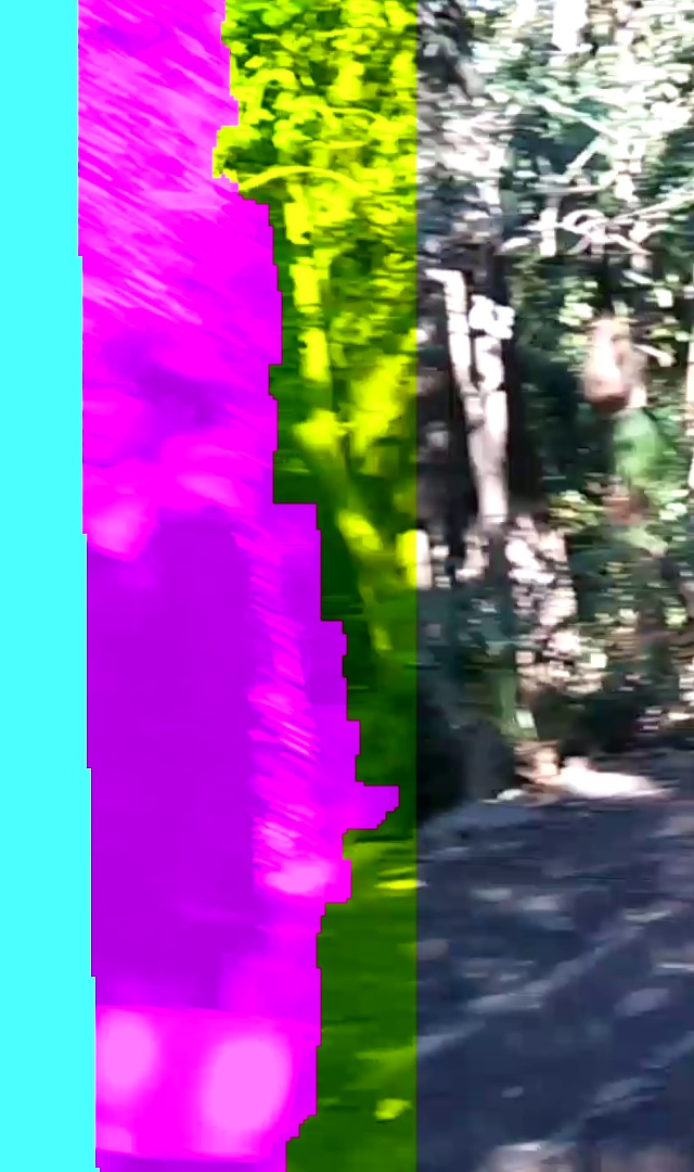
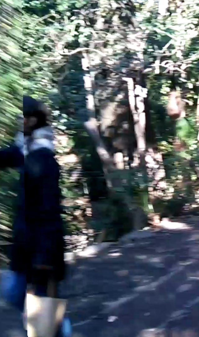
Three images were prepared for both Figure 6 and 7: the result of our stitcher, the image showing the deficit region and the optimal seam, and the result of naive stitching where the deficit region is simply filled by the sub-image. These figures show that our stitcher clearly reduce the unnaturalness of the naive result. It is especially effective for non-planar parts of the scene such as a foreground object or a person walking.

Figure 6: The top panel is the stitching result; the middle panel shows the search region (yellow), the region pasted from the sub-image (pink) and the deficit region (blue); the bottom panel is the result of naive stitching where the deficit region is simply filled by the sub-image. The boundary of the yellow and pink regions corresponds to the optimal seam. While an artificial line is visible in the naive result, it is much less noticeable in the result of our stitcher.

Figure 7: The left panel is the stitching result; the center panel shows the search region (yellow), the region pasted from the sub-image (pink) and the deficit region (blue); the right panel is the result of naive stitching where the deficit region is simply filled by the sub-image. Our stitcher prevents the human face from being cut in half.

VI.2 Standard stitching stabilizer

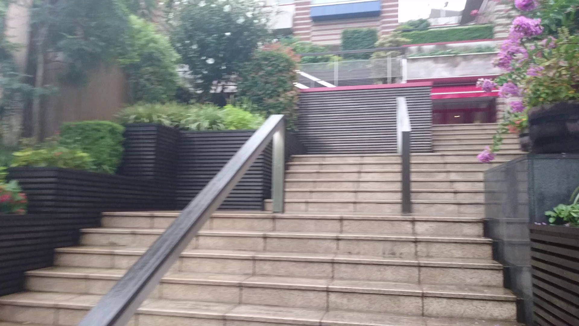
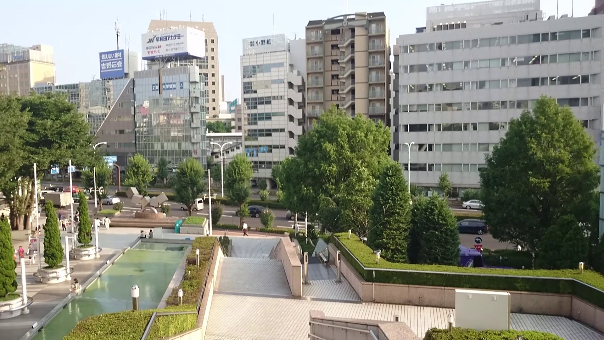
We briefly evaluated the standard stitching stabilizer using three sequences, as shown in Figure 8. These videos were taken by devices without using any stabilization. Because our objective is to achieve a wide AOV, we set the cropping ratio to $90\%$, which corresponds to 1728x972 pixels. The standard choice is $80\%$.

Sequence 1: Walking (upstairs) by Xperia Z3.

Sequence 2: Walking (downstairs) by Xperia Z3.

Sequence 3: Skiing by GoPro HERO3.

Figure 8: Sample sequences. These are typical inputs for video stabilization.

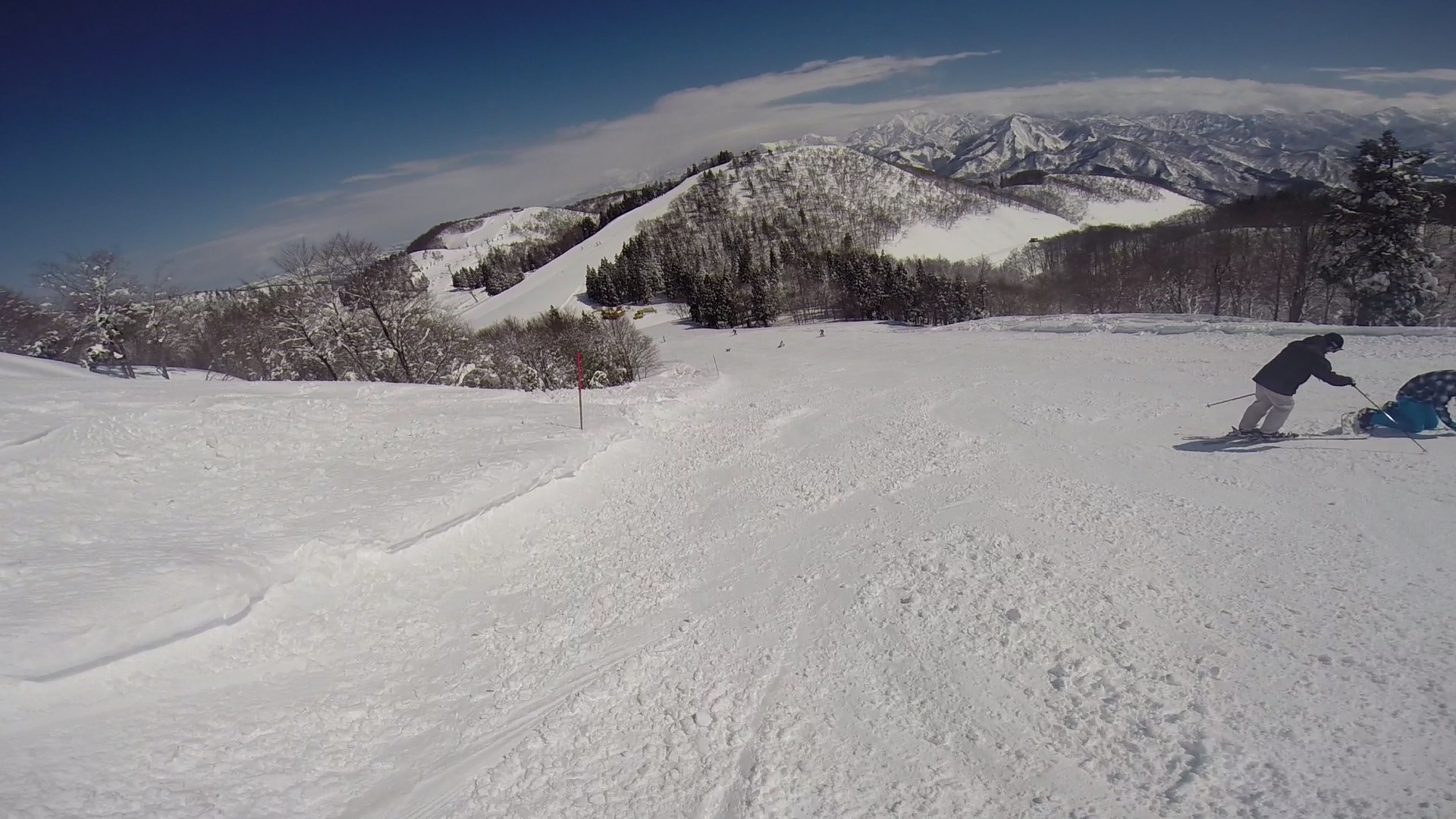
We quantify the improvement in the stitching stabilizer by using the number of frames $n_{f}$ where EnsureInside works. Note that stabilization is imperfect in such frames, because this function introduces artificial shake to the result. We show this in Table 1. The stitching stabilizer reduces $n_{f}$, especially in sequences 1 and 2. Therefore, it works properly.

Table 1: Difference in the number of failed frames $n_{f}$ between the conventional and stitching stabilizer.

		$n_{f}$
	All frames	Conventional	Stitching
Sequence 1	1550	510	176
Sequence 2	1196	456	139
Sequence 3	1608	623	322

VI.3 Hyperlapse

We also set the cropping ratio to 90%, and used the sequences in Figure 8 to evaluate the stitching stabilizer in hyperlapse. Because the filtering algorithm tries to avoid the case where EnsureInside works with full effort, it is difficult to quantify the effect of the stitching stabilizer in the same manner as in the standard case. Instead, we used the final cost value for comparison, since desirable algorithms might choose lower cost results. Our searching algorithm does not guarantee that the cost of the stitching stabilizer is smaller than that of the conventional one, so this should be tested. The result is in Table 2, where we used two parameter sets for filtering. The standard set is $N=64,S=1024,T=6$ and the lite set is $N=64,S=256,T=6$. The cost of the standard set is smaller than that of the lite set, and the cost of the stitching stabilizer is smaller than that of the conventional one, as expected.

Table 2: Difference in the final costs between the conventional and stitching stabilizers.

	$\times 4$ Hyperlapse				$\times 8$ Hyperlapse
	Standard		Lite		Standard		Lite
	Conv.	Stit.	Conv.	Stit.	Conv.	Stit.	Conv.	Stit.
Sequence 1	1932.896	514.436	2156.461	592.443	2377.071	980.790	2420.753	999.795
Sequence 2	2262.367	258.584	2388.724	260.431	1566.641	144.600	1728.087	169.681
Sequence 3	2512.996	991.503	2796.446	1190.797	2525.599	1402.273	2539.572	1590.828

In the supplemental video, we included an exerpt of the result of sequence 2. We prepared the input video with naive frame skipping, the result of the conventional stabilizer, and that of the stitching stabilizer, for $\times 4$ hyperlapse using the standard parameter set. In this video, it is clear that the stitching stabilizer reduces camera shake more effectively than the conventional one does, in hyperlapse.

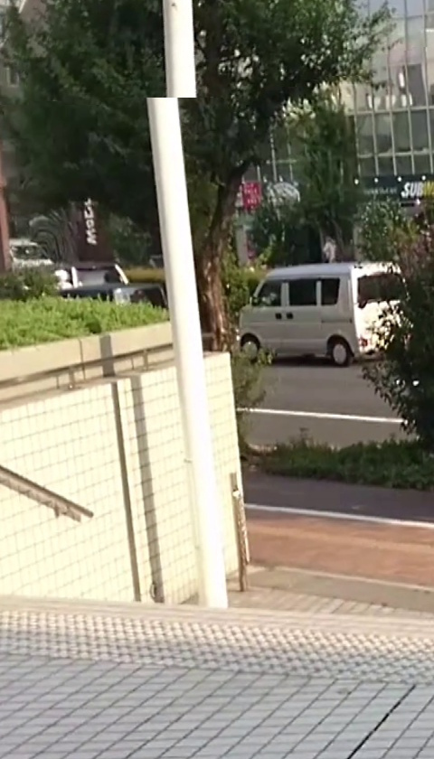
In the result of sequence 2, there is a frame where a pole is cut in half, and we show a part of the frame in Figure 9. It is difficult to stitch perfectly for large or long foreground objects, such as a pole in this example, This is because, the optimal seam cannot circumvent such large objects. Although this is a limitation of the stitching stabilizer, we think it is not a crucial problem for hyperlapse. The reason is following. First, hyperlapse is a kind of fun features. Second, even if this problem occurs in several frames, it is not an easily noticeable defect in first-forwarding videos. For the standard stitching stabilizer, this issue is rare, because the temporal distance between the main and sub-frame is relatively small. In that case, non-planar behavior of foreground objects is manageable in the stitching stabilizer algorithm.

Figure 9: A pole is cut in half in an output frame of sequence 2. The stitching stabilizer does not work perfectly for large or long foreground objects.

For hyperlapse, real-time apps are available for comparison: Microsoft’s mobile app (Microsoft Hyperlapse Mobile) Joshi et al. (2015) and Instagram’s app (Hyperlapse from Instagram) Karpenko (2014). Although it is not a real-time solution, Microsoft’s PC app (Microsoft Hyperlapse Pro) Kopf et al. (2014) might also be a comparison target. We compared the stitching stabilizer with these existing solutions by using several sequences in Figure 10. For the comparison, we use the cropping ratio of 80%, which corresponds to 1536x864, with the standard parameter set. We used two iPhone 6 devices, which were fixed to the same frame, to take videos. This is because Instagram’s app does not accept external files, and we cannot retrieve the input video from the app. Hence, we used the first device only for Instagram’s app. The results for the stitching stabilizer and Microsoft’s apps were created from the same video file taken using the second device. The stitching stabilizer and Instagram’s app perform simple frame skipping, but Microsoft’s apps do not. Therefore, we cannot maintain synchronization between the results in comparison videos.

Sequence 4: Jogging ($\times 4$) by iPhone 6.

Sequence 5: Jogging ($\times 8$) by iPhone 6.

Sequence 6: Driving ($\times 4$) by iPhone 6.

Figure 10: Sequences used for comparison with apps of Microsoft and Instagram. The clips of sequence 4 and 5 are taken at the same day and on the same route. The difference is the setting of hyperlapse, $\times 4$ and $\times 8$.

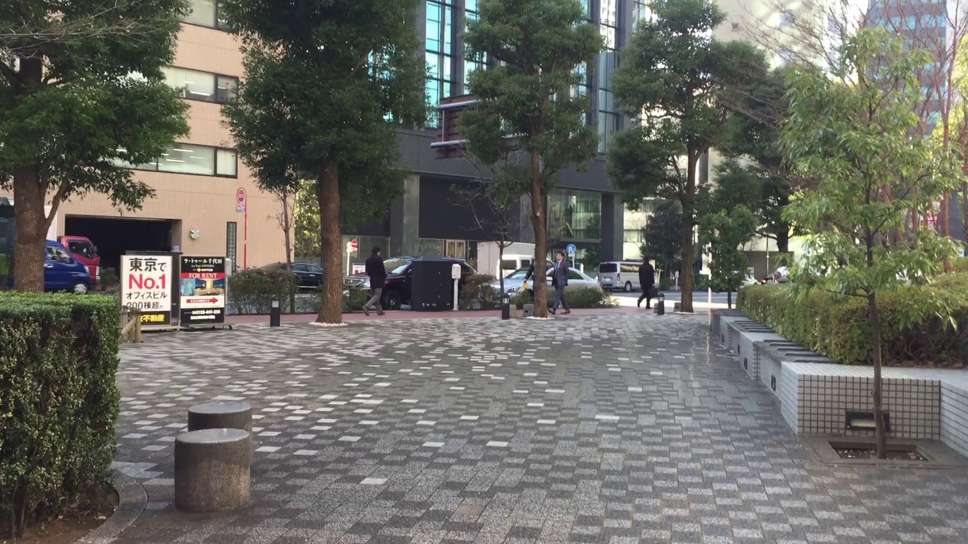
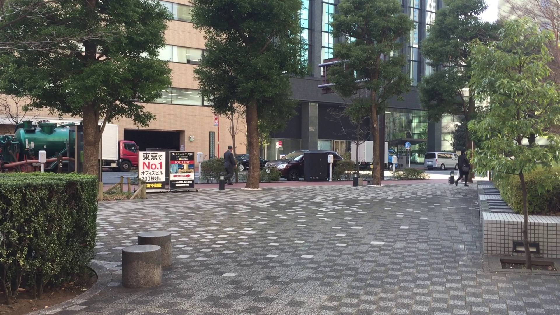
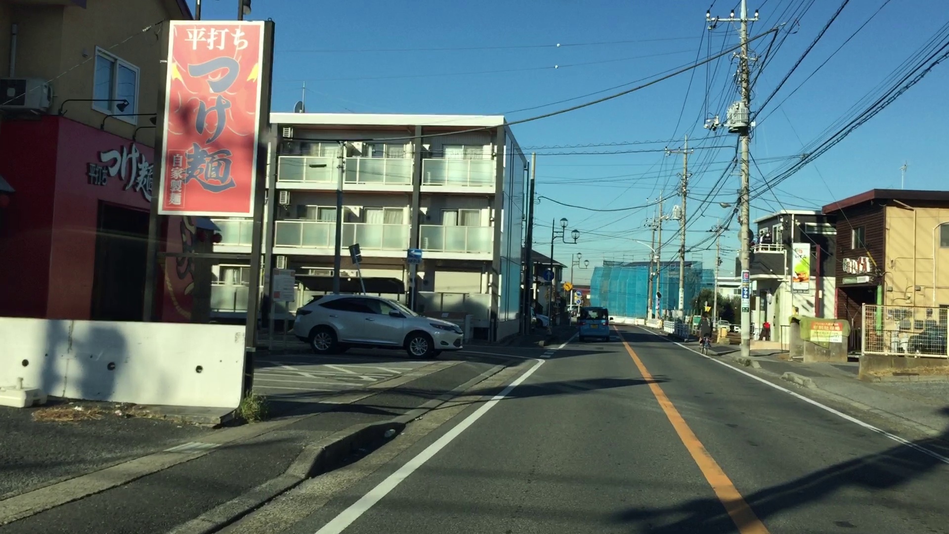
We created $\times 4$ hyperlapse videos for sequences 4 and 6, and $\times 8$ for sequence 5, and compared the results. An exceprt of the most apparent result, that of sequence 4, is included in the supplemental video. Microsoft’s apps, including the PC app, show wobbling and unnatural acceleration and deceleration. Although Instagram’s result is natural, its stabilization is weak. The stitching stabilizer produces a more stabilized result than the mobile apps of Instagram and Microsoft, and the result is more natural than that achieved using Microsoft’s apps. Moreover, at least for this sequence, the result of the stitching stabilizer is even more desirable than that of Microsoft’s PC app, a non real-time solution. The results of the other sequences show essentially the same charasteristic. Hence, we can say that the stitching stabilizer produces a more stabilized and natural output than the existing solutions.

Note that more results of the stitching stabilizer can be found in the supplemental video, where we used 80% cropping with the standard parameter set.

VI.4 Processing time

We measured the processing time of the stitching stabilizer using a commercial device, since it is a crucial issue for real-time solutions. We used Sony’s Xperia Z2 Tablet, which was first launched in the spring of 2014 and has a Qualcomm MSM8974 chipset (Snapdragon 801), as the device. We ran the executable on this device without rooting. Because this was not a new device, if the stitching stabilizer runs in realistic time on this device, it could be used in a variety of recent handsets. We only utilized a CPU with vectorization and parallel threading and did not perform any special tuning for this specific model.

For the standard stitching stabilizer, we measured the first 256 frames for each sequence in Figure 8, and calculated the average FPS. The results are listed in Table 3. The values of FPS here are sufficient enough for 30 FPS video stabilization.

Table 3: Average FPS of the standard stitching stabilizer.

	Process [FPS]
Sequence 1	64.758
Sequence 2	54.124
Sequence 3	49.978

We also measured the time for hyperlapse with the same sequences. The results are summarized in Table 4. The first 256 frames were used for measurement. When there were fewer than 256 output frames, we used all of the frames for the measurement of the main process. The first latency means the time required to create the first output, as explained in subsection V.1. The values of preprocessing FPS are much larger than 30 and fast enough to be run during the video capture. Although the FPS values for main process are large, the first latency also takes a large value. This means we need to wait about half a second to start the hyperlapse with the standard parameter set and about 200 msec with the lite set. There is no explicit threshold for the latency, and it depends on the situation. Hence, the latency should be taken into account when tuning the parameters.

Table 4: Average FPS of hyperlapse with standard and lite parameter sets.

		Main process [FPS]				First latency [msec]
		$\times 4$ Hyperlapse		$\times 8$ Hyperlapse		$\times 4$ Hyperlapse		$\times 8$ Hyperlapse
	Preprocess [FPS]	Standard	Lite	Standard	Lite	Standard	Lite	Standard	Lite
Seq. 1	68.129	76.805	100.210	72.056	107.712	423.615	173.182	752.164	236.283
Seq. 2	69.109	89.350	130.310	64.425	89.270	527.586	245.783	451.672	240.983
Seq. 3	70.602	98.135	100.664	74.716	56.142	551.502	163.183	644.948	239.036

The stitching stabilizer has not yet been fully optimized, and the results listed above was measured on a device that was not new. Therefore, it could be executed with much faster processing time on recent smartphones.

VII Conclusion

We introduced the stitching stabilizer, a software-based video stabilization algorithm that stitches two adjacent input frames together. The stitching process effectively expands the area of input frames and achieves more powerful stabilization than the conventional single-frame algorithm. While the existing methods Litvin et al. (2003); Matsushita et al. (2006); Chen et al. (2008) also do this, their computational cost is too high for embedded systems. The main focus of our algorithm is a real-time process for embedded systems such as smartphones.

We applied the stitching stabilizer to hyperlapse. Because of fast-forwarding, camrera shake is increased in hyperlapse videos. The result of the stitching stabilizer was much smoother than that of the non-stitching stabilizer. We also showed that the stitching stabilizer created a more strongly stabilized and natural output than the frame selection algorithm Joshi et al. (2015) and Instagram’s algorithm Karpenko (2014), which also focus on real-time processing. The results of the stitching stabilizer was even more desirable than that of Kopf et al. Kopf et al. (2014), in some cases.

By using a commercial device, we showed that the processing time of the stitching stabilizer is fast enough for recent smartphones.

The current algorithm works well in many cases. However, there is a fundamental difficulty in some cases, such as when there are large or long foreground objects. In such cases, the simple two-frame stitching algorithm is not very effective. It seems practical to implement a checker that decides whether the scene is suitable for stitching.

Stitching the current frame and the two-frame previous or two-frame next frame, instead of one, might provide stronger stabilization, because we can get a larger input frames by fusing temporally distant frames. While this might introduce unnatural effects, it is worth trying. Stitching more than two frames is another possibility, yet with more computational costs.

For hyperlapse, the stitching stabilizer is further enforced with a frame selection algorithm such as one by Joshi et al. This is a possible direction of research for achieving a higher quality hyperlapse videos.

References

- Litvin et al. (2003) A. Litvin, J. Konrad, and W. C. Karl, in Image and Video Communications and Processing 2003 (SPIE, 2003) pp. 663–674.
- Matsushita et al. (2006) Y. Matsushita, E. Ofek, W. Ge, X. Tang, and H.-Y. Shum, Pattern Analysis and Machine Intelligence, IEEE Transactions on 28, 1150 (2006).
- Chen et al. (2008) B.-Y. Chen, K.-Y. Lee, W.-T. Huang, and J.-S. Lin, Computer Graphics Forum 27, 1805 (2008).
- Kopf et al. (2014) J. Kopf, M. F. Cohen, and R. Szeliski, ACM Trans. Graph. 33, Article No. 78 (2014).
- Karpenko (2014) A. Karpenko, “The technology behind hyperlapse from instagram,” (2014), http://instagram-engineering.tumblr.com/tagged/video-stabilization.
- Joshi et al. (2015) N. Joshi, W. Kienzle, M. Toelle, M. Uyttendaele, and M. F. Cohen, ACM Trans. Graph. 34, Article No. 63 (2015).
- Liu et al. (2009) F. Liu, M. Gleicher, H. Jin, and A. Agarwala, ACM Trans. Graph. 28, Article No. 44 (2009).
- Grundmann et al. (2011) M. Grundmann, V. Kwatra, and I. Essa, in Computer Vision and Pattern Recognition (CVPR), 2011 IEEE Conference on (IEEE, 2011) pp. 225–232.
- Liu et al. (2011) F. Liu, M. Gleicher, J. Wang, H. Jin, and A. Agarwala, ACM Trans. Graph. 30, Article No. 4 (2011).
- Goldstein and Fattal (2012) A. Goldstein and R. Fattal, ACM Trans. Graph. 31, Article No. 126 (2012).
- Liu et al. (2013) S. Liu, L. Yuan, P. Tan, and J. Sun, ACM Trans. Graph. 32, Article No. 78 (2013).
- Karpenko et al. (2011) A. Karpenko, D. Jacobs, J. Baek, and M. Levoy, Digital video stabilization and rolling shutter correction using gyroscopes, Stanford University Computer Science Technical Reports CTSR 2011-03 (Stanford University, 2011).
- Im et al. (2006) J.-A. Im, D.-W. Kim, and K.-S. Hong, in Image Processing, 2006 IEEE International Conference on (IEEE, 2006) pp. 3261–3264.
- Cho and Hong (2007) W.-h. Cho and K.-S. Hong, Consumer Electronics, IEEE Transactions on 53, 833 (2007).
- Liang et al. (2008) C.-K. Liang, L.-W. Chang, and H. H. Chen, Image Processing, IEEE Transactions on 17, 1323 (2008).
- Baker et al. (2010) S. Baker, E. Bennett, S. B. Kang, and R. Szeliski, in Computer Vision and Pattern Recognition (CVPR), 2010 IEEE Conference on (IEEE, 2010) pp. 2392–2399.
- Forssén and Ringaby (2010) P.-E. Forssén and E. Ringaby, in Computer Vision and Pattern Recognition (CVPR), 2010 IEEE Conference on (IEEE, 2010) pp. 507–514.
- Grundmann et al. (2012) M. Grundmann, V. Kwatra, D. Castro, and I. Essa, in Computational Photography (ICCP), 2012 IEEE International Conference on (IEEE, 2012) pp. 1–8.
- Poleg et al. (2015) Y. Poleg, T. Halperin, C. Arora, and S. Peleg, in Computer Vision and Pattern Recognition (CVPR), 2015 IEEE Conference on (IEEE, 2015) pp. 4768–4776.
- Wexler et al. (2004) Y. Wexler, E. Shechtman, and M. Irani, in Computer Vision and Pattern Recognition (CVPR), 2004 IEEE Conference on, Vol. 1 (IEEE, 2004) pp. 120–127.
- Jia et al. (2004) J. Jia, W. Tai-Pang, Y.-W. Tai, and C.-K. Tang, in Computer Vision and Pattern Recognition (CVPR), 2004 IEEE Conference on, Vol. 1 (IEEE, 2004) pp. 364–371.
- Patwardhan et al. (2007) K. Patwardhan, G. Sapiro, M. Bertalmío, et al., Image Processing, IEEE Transactions on 16, 545 (2007).
- Davis (1998) J. Davis, in Computer Vision and Pattern Recognition (CVPR), 1998 IEEE Conference on (IEEE, 1998) pp. 354–360.
- Efros and Freeman (2001) A. A. Efros and W. T. Freeman, in Proceedings of SIGGRAPH ’01 (ACM, 2001) pp. 341–346.
- Kwatra et al. (2003) V. Kwatra, A. Schödl, I. Essa, G. Turk, and A. Bobick, ACM Trans. Graph. 22, 277 (2003).
- Gu et al. (2009) H. Gu, Y. Yu, and W. Sun, in Imaging Systems and Techniques (IST), 2009 IEEE International Workshop on (IEEE, 2009) pp. 159–163.
- Avidan and Shamir (2007) S. Avidan and A. Shamir, ACM Trans. Graph. 26, Article No. 10 (2007).
- Agarwala et al. (2004) A. Agarwala, M. Dontcheva, M. Agrawala, S. Drucker, A. Colburn, B. Curless, D. Salesin, and M. Cohen, ACM Trans. Graph. 23, 294 (2004).
- Dijkstra (1959) E. W. Dijkstra, Numerische mathematik 1, 269 (1959).
- Bergen et al. (1992) J. R. Bergen, P. Anandan, K. J. Hanna, and R. Hingorani, in Computer Vision–ECCV’92 (Springer-Verlag, 1992) pp. 237–252.
- Harris and Stephens (1988) C. Harris and M. Stephens, in Proceedings of the 4th Alvey Vision Conference (Organization Comittee AVC88, 1988) pp. 147–152.
- Orlin (2013) J. B. Orlin, in Proceedings of the forty-fifth annual ACM symposium on Theory of computing (ACM, 2013) pp. 765–774.
- Cormen et al. (2009) T. H. Cormen, C. E. Leiserson, R. L. Rivest, and C. Stein, Introduction to algorithms (MIT Press, 2009).
- Note (1) https://www.youtube.com/watch?v=LmyPXfGZRb0.