Reconstructing the integrated Sachs-Wolfe map with galaxy surveys

Abstract

The integrated Sachs-Wolfe (ISW) effect is a large-angle modulation of the cosmic microwave background (CMB), generated when CMB photons traverse evolving potential wells associated with large scale structure (LSS). Recent efforts have been made to reconstruct maps of the ISW signal using information from surveys of galaxies and other LSS tracers, but investigation into how survey systematics affect their reliability has so far been limited. Using simulated ISW and LSS maps, we study the impact of galaxy survey properties and systematic errors on the accuracy of reconstructed ISW signal. We find that systematics that affect the observed distribution of galaxies along the line of sight, such as photo-$\displaystyle z$ and bias-evolution related errors, have a relatively minor impact on reconstruction quality. In contrast, however, we find that direction-dependent calibration errors can be very harmful. Specifically, we find that in order to avoid significant degradation of our reconstruction quality statistics, direction-dependent number density fluctuations due to systematics must be controlled so that their variance is smaller than $\displaystyle 10^{-6}$ (which corresponds to a 0.1% calibration). Additionally, we explore the implications of our results for attempts to use reconstructed ISW maps to shed light on the origin of large-angle CMB alignments. We find that there is only a weak correlation between the true and reconstructed angular momentum dispersion, which quantifies alignment, even for reconstructed ISW maps which are fairly accurate overall.

I Introduction

As cosmic microwave background (CMB) photons travel from the last scattering surface to our detectors, they can experience a frequency shift beyond that which is guaranteed by the expansion of the universe. This additional effect is a result of the fact that gravitational potential fluctuations associated with large-scale structure (LSS) decay with time when the universe is not fully matter dominated. Consequently, the CMB photons are subject to a direction-dependent temperature modulation which is proportional to twice the rate of change in the potential integrated along the line of sight. This modulation is known as the integrated Sachs-Wolfe (ISW) effect Hu and Sugiyama (1994). Its magnitude in direction $\displaystyle{\bf\hat{n}}$ on the sky was worked out in the classic Sachs-Wolfe paper (Sachs and Wolfe, 1967) to be

$$\left.\frac{\Delta T}{\bar{T}}\right|_{ISW}({\bf\hat{n}})=\frac{2}{c^{2}}\int_{t_{*}}^{t_{0}}dt\,\frac{\partial\Phi(\mathbf{r},t)}{\partial t},$$ (1)

where $\displaystyle t_{0}$ is the present time. $\displaystyle t_{\star}$ is that of recombination, $\displaystyle c$ is the speed of light, $\displaystyle\mathbf{r}$ is the position in comoving coordinates, and $\displaystyle\Phi$ is the gravitational potential.

The ISW effect introduces a weak additional signal at very large scales (low multipoles) in the CMB angular power spectrum. It carries important information about dark energy Bean and Dore (2004); Weller and Lewis (2003), particularly its clustering properties that are often parametrized by the dark energy speed of sound. It also potentially offers useful information about the the nature of dark energy, as modified gravity theories have unique ISW signatures Song et al. (2007). However, the fact that the largest CMB multipoles are subject to cosmic variance severely limits how much information can be gleaned from the ISW given the CMB temperature measurements alone.

We are able to observe the ISW effect because the dependence of the ISW signal on the time derivative of the potential results in a large-angle cross-correlation between LSS tracers and CMB temperature. This was first pointed out by Crittenden & Turok Crittenden and Turok (1996), who further suggested cross-correlation between CMB temperature anisotropy $\displaystyle(\delta T/T)_{\rm ISW}({\bf\hat{n}})$ and galaxy positions, $\displaystyle(\delta N/N)({\bf\hat{n}^{\prime}})$, as a statistic through which to detect the ISW effect. This cross-correlation signal was detected shortly thereafter (Boughn and Crittenden, 2004) and was later confirmed by many teams who found cumulative evidence of about $\displaystyle 4\sigma$ using a number of different LSS tracers Fosalba et al. (2003); Nolta et al. (2004); Corasaniti et al. (2005); Padmanabhan et al. (2005); Vielva et al. (2006); McEwen et al. (2007); Giannantonio et al. (2006); Cabre et al. (2007); Rassat et al. (2007); Giannantonio et al. (2008); Ho et al. (2008); Xia et al. (2009); Giannantonio et al. (2012); Ade et al. (2014, 2015a). Comprehensive surveys of recent results can be found in Refs. Dupe et al. (2011); Giannantonio et al. (2012); Ade et al. (2015a). While the detection of the ISW effect itself provides independent evidence for dark energy at high statistical significance, prospects for using it to constrain the cosmological parameters are somewhat limited (Hu and Scranton, 2004).

The ISW map, $\displaystyle(\delta T/T)_{\rm ISW}({\bf\hat{n}})$, is also of interest in its own right. By assuming a cosmological model, one can construct an estimator using theoretical cross-correlations in combination with LSS data. Because the ISW signal represents a late-universe contribution to the CMB anisotropy, measuring and subtracting it from observed temperature fluctuations would allow us to isolate the (dominant) early-universe contributions to the CMB. If this procedure could be done reliably, it would have immediate implications for our understanding of the cosmological model.

For example, the ISW signal has been identified as a potential contributor to large-angle CMB features which have been reported to be in tension with the predictions of $\displaystyle\Lambda$CDM Schwarz et al. (2015). A reconstructed ISW map would clarify whether some component of the CMB anomalies (discussed further below in Sec. V) become stronger or weaker when evaluated on the early-universe-only contribution to the CMB. A few studies Francis and Peacock (2010); Rassat et al. (2013) have already explored this. To study the impact of ISW contributions on CMB anomalies, Ref. Rassat et al. (2013) uses WMAP data with 2MASS and NVSS, while Ref. Francis and Peacock (2010) uses 2MASS alone.

The late-time ISW also provides a contaminant to the measurement of primordial non-Gaussianity from CMB maps. Because both the ISW effect and gravitational lensing trace LSS, they couple large- and small-scale modes of the CMB, resulting in a nonprimordial contribution to the bispectrum. Recent analyses Ade et al. (2015b) have corrected for this by including a theoretical template for the ISW-lensing bispectrum in primordial $\displaystyle f_{NL}$ analyses. Reconstructing and subtracting the ISW contribution from the CMB temperature maps could provide an alternative method for removing ISW-lensing bias when studying primordial non-Gaussianity Kim et al. (2013).

More generally, understanding how reliably the ISW map can be reconstructed from large-scale structure information impacts our understanding of how the late universe affects our view of the primordial CMB sky.

Before reconstruction can be done reliably, however, we must understand how systematics associated with the input data impact the ISW estimator’s accuracy. Previous works have explored this to some extent, looking at how reconstruction quality is affected by the inclusion of different input data sets Manzotti and Dodelson (2014); Ade et al. (2015a); Bonavera et al. (2016), masks Ade et al. (2015a); Bonavera et al. (2016) and, to a limited degree, the influence of uncertainties in cosmological and bias models Bonavera et al. (2016). Additionally, Ref. Afshordi (2004) studied how systematics like redshift uncertainties and photometric calibration change the signal to noise of the ISW effect’s detection. That being said, there remain a number of systematics inherent to galaxy survey data which have not yet been subject to detailed analysis in the context of ISW map reconstruction. We aim to address this.

In this paper, we use simulated ISW and LSS maps to identify which survey properties are important for ISW reconstruction and to quantify their effects on the reconstructed maps. We begin by studying how survey depth, redshift binning strategy, and the minimum measured multipole $\displaystyle\ell_{\rm min}$ influence reconstruction quality in the absence of systematics. Using these results as a baseline, we then explore two broad classes of systematics: ways one can mismodel the redshift distribution of LSS sources, and direction-dependent photometric calibration errors that can result from, for example, contamination by stars. We also briefly discuss the implications of our results for analysis of whether the ISW signal contributes to the observed alignments between large-angle multipoles of the CMB temperature map.

The paper is organized as follows. In Sec. II we discuss our general procedure for the ISW map reconstruction and assessment of the accuracy in this procedure. In Sec. III, we describe the properties of the surveys that we will consider, while in Sec. IV, we discuss the effect of various systematic errors on the ISW map reconstruction. We conclude in Sec. VI.

II Methods

We perform a number of studies examining how survey properties and systematics affect the accuracy of reconstructed ISW maps. These studies all follow this general pipeline:

• Select a fiducial cosmological model and specifications of the LSS survey.

• Compute the “true” angular cross-power $\displaystyle C_{\ell}^{XY}$ for ISW and LSS maps, assuming the fiducial cosmology and survey specifications.

• Use the true $\displaystyle C_{\ell}^{XY}$ to generate correlated Gaussian realizations of the true ISW signal and corresponding LSS maps.

• If applicable, postprocess the galaxy maps to model direction-dependent systematic effects.

• Construct an estimator for the ISW signal using the simulated galaxy maps and a set of “model” $\displaystyle C_{\ell}^{XY}$ which may or may not match those used to generate the simulations.

• Compare the reconstructed ISW signal to the true ISW map and evaluate the accuracy of the reconstruction.

This section will introduce some of the theoretical tools needed for this analysis.

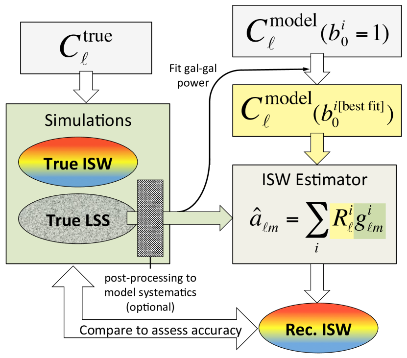
Figure 1: Flowchart of reconstruction pipeline.

II.1 Theoretical cross-correlations

The angular cross-power between ISW and galaxy maps serves as input for both the simulation and reconstruction processes used in the following sections. Given maps $\displaystyle X$ and $\displaystyle Y$, the expression for the angular cross-power between them is

$$C_{\ell}^{XY}=\frac{2}{\pi}\int dk\,k^{2}\,P(k)\,I_{\ell}^{X}(k)\,I_{\ell}^{Y}(k)$$ (2)

where $\displaystyle P(k)$ is the matter power spectrum at $\displaystyle z=0$, and the transfer function $\displaystyle I_{\ell}^{X}(k)$ is written

$$I_{\ell}^{X}(k)\equiv\int_{0}^{\infty}\,dz\,D(z)\,W^{X}(z,k)\,j_{\ell}(kr).$$ (3)

Here, $\displaystyle r\equiv r(z)$ represents comoving radius; $\displaystyle j_{\ell}(x)$ is a spherical Bessel function; and $\displaystyle D(z)$, which is normalized to one at $\displaystyle z=0$, describes the linear growth of matter fluctuations. The function $\displaystyle W^{X}(k,z)$ is a tracer-specific window function that encapsulates the relationship between the tracer $\displaystyle X$ and underlying dark matter fluctuations $\displaystyle\delta$. The tracers relevant to our studies are the ISW signal and galaxy number density.

The ISW window function is

$$W^{\rm ISW}(z,k)=\left[\Theta(z_{\rm max}-z)\right]\,\left[\frac{3H_{0}^{2}\Omega_{m}}{c^{2}k^{2}}\right]\left(1-f(z)\right),$$ (4)

where $\displaystyle\Theta$ is the Heaviside step function. In this expression, the term in square brackets comes from when the Poisson equation is used to relate potential fluctuations to dark matter density, $\displaystyle\Omega_{m}$ is the matter density in units of the critical density, and $\displaystyle H_{0}$ is the present-day Hubble parameter. The appearance of the growth rate $\displaystyle f(z)\equiv d\ln D/d\ln a$ comes from the time derivative in Eq. (1). To compute the full ISW contribution, one would integrate to the redshift of recombination, $\displaystyle z_{\rm max}=z_{\star}$. In this work, though, we are interested only in the late ISW effect, so we can set $\displaystyle z_{\rm max}=15$ without a loss in accuracy.

Each survey (and each redshift bin within a given survey) will have its own window function. For a map of galaxy number density fluctuations, it is

$$W^{\rm gal}(z,k)=b(z)\,\frac{dn}{dz}.$$ (5)

In this expression, $\displaystyle b(z)$ represents linear bias, which we assume is scale independent. The function $\displaystyle dn/dz$ describes the redshift distribution the observed sources, encapsulating information about how their physical density varies with redshift as well as survey volume and selection effects. It is normalized so it integrates to one. Galaxy shot noise is included by adding a contribution to its autopower spectrum,

$$C_{\ell}^{\rm gal-gal}\rightarrow C_{\ell}^{\rm gal-gal}+\bar{n}^{-1}$$ (6)

where $\displaystyle\bar{n}$ is the average number density of sources per steradian. In summary, to simulate a given galaxy survey, we need $\displaystyle b(z)$, describing how clustered its sources are relative to dark matter; $\displaystyle dn/dz$, describing how the observed sources are distributed along the line of sight; and $\displaystyle\bar{n}$, the average number density of sources per steradian.

For $\displaystyle\ell>20$, we use the Limber approximation to compute $\displaystyle C_{\ell}^{XY}$. This dramatically reduces the computation time and gives results that are accurate to within about 1% LoVerde and Afshordi (2008). In this approximation, the cross-correlations become

$$C_{\ell}^{XY}=\int dz\frac{H(z)\,D^{2}(z)}{c\,r^{2}(z)}\,\left[P(k)\,W^{X}(k,z)\,W^{Y}(k,z)\right]_{k=k_{\ell}},$$ (7)

where $\displaystyle k_{\ell}=(\ell+\tfrac{1}{2})/r(z)$ and $\displaystyle H(z)$ is the Hubble parameter.

We developed an independent code to calculate the cross-power spectra $\displaystyle C_{\ell}^{XY}$ and have extensively tested its accuracy for various survey redshift ranges against the publicly available CLASS code Lesgourgues (2011).

II.2 Simulating LSS maps

As we care only about large-angle ($\displaystyle\ell\lesssim 100$) features, we model the ISW signal and galaxy number density fluctuations as correlated Gaussian fields. To simulate them, we compute the relevant angular auto- and cross-power $\displaystyle C_{\ell}$’s and then use the synalm function from Healpy Gorski et al. (2005) to generate appropriately correlated sets of spherical harmonic coefficients $\displaystyle g_{\ell m}$. These components are defined via the spherical harmonic expansion of the number density of sources in the $\displaystyle i$th LSS map,

$$\left[\frac{\delta N}{N}\right]^{i}({\bf\hat{n}})=\sum_{\ell m}\,g_{\ell m}^{i}\,Y_{\ell m}({\bf\hat{n}}).$$ (8)

For each study using simulated maps, we generate 10,000 map realizations. We use Healpix with NSIDE=32 and compute $\displaystyle C_{\ell}$ up to $\displaystyle\ell_{\rm max}=95$, guided by the relation $\displaystyle\ell_{\rm max}=3({\rm\tt NSIDE})-1$. Unless we state otherwise, our ISW reconstructions include multipole information down to $\displaystyle\ell_{\rm min}=2$.

All of our analyses are for full-sky data and our fiducial cosmological model is $\displaystyle\Lambda$CDM, with parameter values from best-fit Planck 2015, $\displaystyle\{\Omega_{c}h^{2},\Omega_{b}h^{2},\Omega_{\nu}h^{2},h,n_{s}\}=\{0.1188,0.0223,0,0.6774,0.9667\}$.

II.2.1 Fiducial survey

We model our fiducial galaxy survey on what is expected for Euclid Laureijs et al. (2011). With its large sky coverage and deep redshift distribution the Euclid survey has been identified as a promising tool for ISW detection Afshordi (2004); Douspis et al. (2008) and it is reasonable to assume that these properties will also make it a good data set to use for ISW reconstruction. We therefore adopt the redshift distribution used in Ref. Martinet et al. (2015),

$$\frac{dn}{dz}=\frac{3}{2z_{0}^{2}}z^{2}\,\exp{\left[-(z/z_{0})^{-1.5}\right]}$$ (9)

which has a maximum at $\displaystyle z_{\rm peak}\simeq 1.21z_{0}$. We adopt $\displaystyle z_{0}=0.7$ and $\displaystyle\bar{n}=1\times 10^{9}$. For binning studies (see Sec. III.2) we assume a photo-$\displaystyle z$ redshift uncertainty of $\displaystyle\sigma(z)=0.05(1+z)$. Our fiducial bias is $\displaystyle b(z)=1$. We explicitly state below whenever these fiducial values are varied for our tests.

II.3 ISW estimation

We use the optimal estimator derived in Ref. Manzotti and Dodelson (2014) to reconstruct the ISW signal from LSS maps. Because we are interested in quantifying the impact of galaxy survey systematics, in this work we focus on the case where only galaxy maps are used as input. We thus neglect the part of the estimator that includes CMB temperature information and write

$$\hat{a}_{\ell m}^{\rm ISW}=\sum_{i}^{n}R_{\ell}^{i}g_{\ell m}^{i}.$$ (10)

Here $\displaystyle\hat{a}_{\ell m}$ is the optimal estimator for the ISW map component, $\displaystyle g_{\ell m}^{i}$ is the observed spherical component of LSS tracer $\displaystyle i$, and $\displaystyle n$ is the number of LSS tracers considered. The operator

$$R_{\ell}^{i}\equiv-N_{\ell}[D_{\ell}^{-1}]_{{\rm ISW-}i}$$ (11)

is the reconstruction filter applied to the $\displaystyle i$th LSS map. It is constructed from the covariance matrix $\displaystyle D_{\ell}$ between ISW and LSS tracers,

$$D_{\ell}=\left(\begin{array}[]{cccc}C_{\ell}^{\rm{ISW,ISW}}&C_{\ell}^{\rm{LSS}_{1}\rm{,ISW}}&\cdots&C_{\ell}^{\rm{LSS}_{n}\rm{,ISW}}\\ C_{\ell}^{\rm{LSS}_{1}\rm{,ISW}}&C_{\ell}^{\rm{LSS}_{1}\rm{,LSS}_{1}}&\cdots&C_{\ell}^{\rm{LSS}_{1}\rm{,LSS}_{n}}\\ \vdots&\vdots&\ddots&\vdots\\ C_{\ell}^{\rm{LSS}_{n}\rm{,ISW}}&C_{\ell}^{\rm{LSS}_{1}\rm{,LSS}_{n}}&\cdots&C_{\ell}^{\rm{LSS}_{n}\rm{,LSS}_{n}}\\ \end{array}\right).$$ (12)

The term $\displaystyle N_{\ell}^{-1}\equiv(D_{\ell}^{-1})_{11}$ estimates the reconstruction variance.

Note that for reconstruction using a single LSS map this reduces to a Wiener filter.

$$\hat{a}_{\ell m}^{\rm{ISW}}\stackrel{{\scriptstyle\mathclap{\mbox{\scriptsize single LSS}}}}{{\hskip 12.80365pt\longrightarrow\hskip 12.80365pt}}\frac{C_{\ell}^{\rm ISW-gal}}{C_{\ell}^{\rm gal-gal}}g_{\ell m}.$$ (13)

In the subsequent discussion, we will refer to the correlations appearing in $\displaystyle D_{\ell}$ (and thus the reconstruction filters $\displaystyle R_{\ell}^{i}$) as $\displaystyle C_{\ell}^{\rm model}$. This is to distinguish them from the correlations used to generate the simulations, which we will call $\displaystyle C_{\ell}^{\rm true}$. We adopt this convention because if we were reconstructing the ISW signal based on real data, $\displaystyle C_{\ell}^{\rm true}$ would be the correlations determined by the true underlying physics of the universe, while $\displaystyle C_{\ell}^{\rm model}$ would be computed theoretically based on our best knowledge of cosmological parameters and the properties of the input LSS tracers.

Setting $\displaystyle C_{\ell}^{\rm model}=C_{\ell}^{\rm true}$ represents a best-case scenario where we have perfect knowledge of the physics going into the calculations outlined in Sec. II.1. Incorrect modeling will break that equality, causing the estimator in Eq. (10) to become suboptimal. Our analysis of LSS in Sec. IV systematics will fundamentally be an examination of how different manifestations of this kind of $\displaystyle C_{\ell}^{\rm model}\neq C_{\ell}^{\rm true}$ mismatch impact reconstruction.

II.4 Fitting for effective galaxy bias

Our pipeline actually contains an additional step, which as we will see in later sections, helps protect against some systematics; before constructing the ISW estimator, we fit the galaxy maps for a constant bias.

When performing this procedure, the first step of our reconstruction process is to measure the galaxy autopower spectrum from the observed galaxy map, $\displaystyle C_{\ell}^{\rm gal(obs)}$. This will be subject to cosmic variance scatter about $\displaystyle C_{\ell}^{\rm gal(true)}$ and so will be realization dependent. We then perform a linear fit for a constant $\displaystyle\bar{b}$ satisfying

$$C_{\ell}^{\rm gal(obs)}=\bar{b}^{2}\,C_{\ell}^{\rm gal(model)}.$$ (14)

We then scale the model power spectra:

$$\displaystyle C_{\ell}^{\rm gal}\quad \displaystyle\rightarrow\quad\bar{b}^{2}\,C_{\ell}^{\rm gal},$$

$$\displaystyle C_{\ell}^{\rm gal-ISW}\quad \displaystyle\rightarrow\quad\bar{b}\,C_{\ell}^{\rm gal-ISW},$$ (15)

$$\displaystyle C_{\ell}^{{\rm gal}_{i}-{\rm gal}_{j}}\quad \displaystyle\rightarrow\quad\bar{b}^{i}\,\bar{b}^{j}\,C_{\ell}^{{\rm gal}_{i}-{\rm gal}_{j}}.$$

If there are no systematics affecting our measurements, $\displaystyle C_{\ell}^{\rm gal(true)}=C_{\ell}^{\rm gal(model)}$, so $\displaystyle\bar{b}$ will be close to 1. When a galaxy bias is modeled as a constant, $\displaystyle b_{0}$, for each galaxy map, this scaling will exactly correct for any mismatch between the value used in the simulations and that in the model used to construct the ISW estimator:

$$\bar{b}=b_{0}^{\rm true}/b_{0}^{\rm model}.$$ (16)

Outside the case of constant bias, there is not a direct correspondence between $\displaystyle\bar{b}$ and the paramters of the bias model. (It corresponds to the ratio between weighted averages of $\displaystyle b(z)^{\rm true}$ and $\displaystyle b(z)^{\rm model}$.) However, the procedure for fitting for and scaling by $\displaystyle\bar{b}$ is well defined and makes our estimator robust against systematics which shift $\displaystyle C_{\ell}$’s by a multiplicative constant, including mismodeled $\displaystyle b(z)$ and $\displaystyle dn/dz$. We will demonstrate this in Sec. IV.1.

II.5 Evaluating reconstruction accuracy

We will use two statistics to quantify the accuracy of reconstructed ISW maps. Primarily, we will use the correlation coefficient between the true ISW signal $\displaystyle T^{\rm ISW}({\bf\hat{n}})$ and the reconstructed ISW map $\displaystyle T^{\rm rec}({\bf\hat{n}})$. For a given realization we compute this as

$$\rho=\frac{\langle T^{\rm ISW}T^{\rm rec}\rangle_{\rm pix}}{\sigma_{\rm ISW}\sigma_{\rm rec}},$$ (17)

where $\displaystyle\langle\rangle_{\rm pix}$ indicates an average over pixels, and $\displaystyle\sigma_{X}$ is the variance of map $\displaystyle X$.

We can approximate the theoretical expectation value for $\displaystyle\rho$ using the cross-power between maps,

$$\displaystyle\langle\rho\rangle=\frac{\sum_{\ell i}(2\ell+1)R_{\ell}^{i}C_{\ell}^{{\rm ISW}-i}}{\langle\sigma_{\rm rec}\rangle\langle\sigma_{\rm ISW}\rangle},$$ (18)

where the indices $\displaystyle i$ and $\displaystyle j$ label LSS maps and

$$\displaystyle\langle\sigma_{\rm ISW}\rangle \displaystyle=\sqrt{\sum_{\ell}\,(2\ell+1)\,C_{\ell}^{\rm ISW}}$$ (19)

$$\displaystyle\langle\sigma_{\rm rec}\rangle \displaystyle=\sqrt{\sum_{\ell ij}\,(2\ell+1)\,R_{\ell}^{i}R_{\ell}^{j}C_{\ell}^{ij}}$$ (20)

are the standard deviations of the temperature maps.In deriving this expression, we assumed $\displaystyle\langle\sigma^{-1}\rangle=\langle\sigma\rangle^{-1}$ and that the various factors in this expression are uncorrelated. We will see later that this is a reasonably accurate approximation to make, as it gives values which are in good agreement with simulation results.

One can see by examining Eqs. (17) and (18) that $\displaystyle\rho$ is sensitive to the reconstruction of phases but insensitive to changes in the overall amplitude of the reconstructed ISW map. Because of this, though $\displaystyle\rho\rightarrow 1$ is generally indicative of a more accurate reconstruction, this quantity does not capture all important information about reconstruction quality. We therefore also consider a complementary statistic which is sensitive to amplitude, defined

$$s=\frac{\langle(T^{\rm ISW}-T^{\rm rec})^{2}\rangle_{\rm pix}^{1/2}}{\sigma_{\rm ISW}}.$$ (21)

The quantity $\displaystyle s$ measures how the average size of errors in the reconstructed signal compares to that of fluctuations in the true ISW map. As with $\displaystyle\rho$, we can compute its expectation value,

$$\langle s\rangle=\frac{\sqrt{\langle\sigma_{\rm rec}\rangle^{2}+\langle\sigma_{\rm ISW}\rangle^{2}-2\,\sum_{\ell i}\,(2\ell+1)\,R_{\ell}^{i}C_{\ell}^{{\rm ISW}-i}}}{\langle\sigma_{\rm ISW}\rangle}.$$ (22)

Because the bias-fitting procedure discussed in Sec. II.4 corrects for amplitude differences, for most of the scenarios we study, $\displaystyle\rho$ and $\displaystyle s$ effectively contain the same information. For this reason, we will primarily use $\displaystyle\rho$ as our quality statistic and will only show results for $\displaystyle s$ when it contributes new insight.

Throughout this paper we will use angled brackets to indicate the theoretical expectation values for these statistics, and an overbar to indicate averages computed from simulations.

III Results I: The effect of survey properties

Before studying the effects of systematics, it is instructive to explore how LSS survey properties impact ISW signal reconstruction in the ideal, $\displaystyle C_{\ell}^{\rm model}=C_{\ell}^{\rm true}$, scenario. This has already been done to some extent in Refs. Manzotti and Dodelson (2014), Ade et al. (2015a), and Bonavera et al. (2016).

Our studies in this section will serve two primary purposes. First, they will provide a straightforward demonstration of our pipeline and the reconstruction quality statistics introduced in Sec. II.5. More importantly, they will serve as a baseline for our analysis of systematics in Sec. IV: Our goal is not to find optimized survey properties for ISW signal reconstruction, though our results might serve as a rough guide for doing so. Rather, we want to study how shifting, for example, survey depth or redshift binning strategy affects ISW reconstruction in the best-case scenario (with no systematic errors) so that we can better understand the impact of what happens when those errors are introduced.

III.1 Varying survey depth

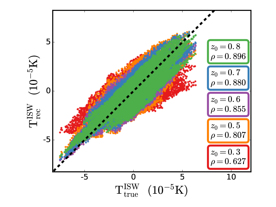
Figure 2: Scatter plot comparing the true (simulated) ISW signal, on the horizontal axis, to the reconstructed ISW signal, on the vertical axis, for a single realization assuming each of five different depths of the survey. Each data point corresponds to one pixel on an NSIDE=32 map. If there was a perfect reconstruction, all points would fall on the dotted gray line.

The first property we examine is survey depth. We model this by changing the value of $\displaystyle z_{0}$ in our fiducial $\displaystyle dn/dz$ [Eq. (9)] while holding all other survey properties fixed. We look at values $\displaystyle\Delta z=\pm 0.1$ on either side of our fiducial $\displaystyle z_{0}=0.7$, plus a redshift distribution comparable to DES Becker et al. (2015) with $\displaystyle z_{0}=0.5$ and the even-shallower $\displaystyle z_{0}=0.3$.

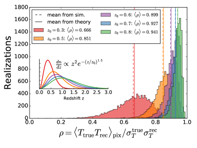
Figure 3: Histograms of the correlation between true and reconstructed ISW maps $\displaystyle\rho$ (left panel), and the typical size of residuals relative to that of the true ISW map fluctuations $\displaystyle s$ (right panel). These plots show the results of 10,000 simulations for surveys of various depths, with their $\displaystyle dn/dz$ distributions shown in arbitrary units as an inset in the left plot. The solid and dashed vertical lines show the theoretical expectation value and measured average, respectively, for the statistic in question.

Figure 2 shows a pixel-by-pixel comparison between the reconstructed and true ISW signal for a single representative realization. We can see that the deeper surveys have data-points more tightly clustered around the $\displaystyle T^{\rm ISW}_{\rm rec}=T^{\rm ISW}_{\rm true}$ diagonal and correspondingly higher values of $\displaystyle\rho$.

We find that this pattern holds, if noisily, in the full ensemble of simulated maps. Figure 3 shows histograms of $\displaystyle\rho$ for the same surveys, with their $\displaystyle dn/dz$ distributions shown in an inset. In it, the sample average $\displaystyle\bar{\rho}$ and theoretical expectation value $\displaystyle\langle\rho\rangle$ are plotted as dashed and solid vertical lines, respectively. We find that though $\displaystyle\langle\rho\rangle$ tends to be lower than $\displaystyle\bar{\rho}$, the difference between them is much smaller than the scatter in the data, and that the ordering of $\displaystyle\langle\rho\rangle$ values for the different surveys is consistent with the results from simulations. We take this to mean that the more computationally efficient $\displaystyle\langle\rho\rangle$ is a slightly biased but reasonably reliable indicator of the ISW reconstruction quality.

Looking at the data, we also note that the scatter in the individual $\displaystyle\rho$ distributions is large compared to the difference between their mean values. This tells us that, while $\displaystyle\langle\rho\rangle$ (or $\displaystyle\bar{\rho}$) values succeed in predicting how ISW reconstruction quality from different surveys will compare on average, they are a relatively poor predictor of how surveys will compare for any individual realization.

For illustrative purposes, in Fig. 3, we also show a histogram for the values of statistic $\displaystyle s$ which, recall, is mainly sensitive to the amplitude accuracy in the map reconstruction – measured from the same simulations. We see that (as expected) surveys with larger $\displaystyle\bar{\rho}$ have smaller $\displaystyle\bar{s}$ and that the surveys with $\displaystyle\bar{\rho}\sim 0.9$ correspond to $\displaystyle\bar{s}\sim 0.4$. This tells us that even in the best maps that we study here, errors in the reconstructed ISW temperature are a little over one-third of the amplitude of true ISW signal fluctuations.

We keep the mean source number density $\displaystyle\bar{n}$ fixed for this analysis, so that any differences we observe in reconstruction quality are due only to how the redshift distributions are sampled, not to the fact that a deeper survey will observe a larger number of sources. We argue that this is well motivated because the only way $\displaystyle\bar{n}$ enters our calculations is via shot noise, and we have set it to a large enough value so that its contributions are negligible on large, ISW-relevant scales.

III.2 Redshift binning strategy

Here we study how different strategies for binning galaxy data affect the reconstruction. For each bin with $\displaystyle z_{i}\leq z<z_{i+1}$, we model the redshift distribution by weighting the survey’s overall distribution $\displaystyle dn^{\rm tot}/dz$ with a window function $\displaystyle F_{i}(z)$ and scale the total number density accordingly:

$$\displaystyle\frac{dn^{i}}{dz} \displaystyle=\frac{\displaystyle\frac{dn^{\rm tot}}{dz}\,F_{i}(z)}{\displaystyle\int_{0}^{\infty}\displaystyle\frac{dn^{\rm tot}}{dz}\,F_{i}(z)\,dz},$$ (23)

$$\displaystyle\bar{n}^{i} \displaystyle=\bar{n}^{\rm tot}\times\left[\int_{0}^{\infty}\displaystyle\frac{dn^{\rm tot}}{dz}\,F_{i}(z)\,dz\right].$$ (24)

We can then compute $\displaystyle C_{\ell}^{XY}$ using the expressions in Sec. II.1, treating each redshift bin as an individual map ($\displaystyle X$ or $\displaystyle Y$).

Photometric redshift uncertainties will cause sharp divisions in observed redshift to be smoothed when translated to spectroscopic redshift. As in Ref. Manzotti and Dodelson (2014) we therefore model the effect of photometric uncertainties $\displaystyle\sigma(z)$ via

$$F_{i}(z)=\frac{1}{2}\left[{\rm erfc}\,\left(\frac{z_{i}-z}{\sigma(z)\sqrt{2}}\right)-{\rm erfc}\,\left(\frac{z_{i+1}-z}{\sigma(z)\sqrt{2}}\right)\right],$$ (25)

which effectively acts as a smoothed top-hat window in $\displaystyle z$. We use the standard form for photometric-redshift uncertainty

$$\sigma(z)=\sigma_{z0}\times(1+z).$$ (26)

For reference, Euclid forecasts consider $\displaystyle\sigma_{z0}=0.05$ a requirement and give $\displaystyle\sigma_{z0}=0.03$ as a reach goal Cimatti et al. (2009); Laureijs et al. (2011).

In order to understand how binning affects ISW reconstruction, we split our fiducial redshift distribution into the six bins shown in Fig. 4 and compute all possible auto- and cross-correlations between them. We then use the relations from Ref. Hu (1999) to compute $\displaystyle C_{\ell}^{XY}$ for cases where two or more adjacent bins are merged.

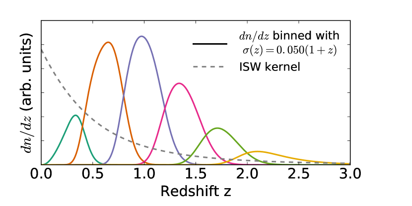
Figure 4: Un-normalized redshift distributions for the six redshift bins studied, with photometric-redshift uncertainty $\displaystyle\sigma(z)=0.05(1+z)$. Because these distributions are not yet normalized (they neglect the denominator of Eq. (23)), the area under the curves gives an idea of the relative number of galaxies in each bin. The dotted line shows the ISW kernel in arbitrary units.

To check that our understanding of reconstruction statistics holds for surveys with multiple redshift bins, we simulated 10,000 map realizations for three configurations: the one-bin fiducial case, the six-bin case, and a three-bin case with edges at $\displaystyle z\in[0,0.8,1.6,3.5]$. For all of these, we used $\displaystyle\sigma_{z0}=0.05$. The results, shown in Fig. 5, reveal that though binning slightly improves the reconstruction quality, it does not dramatically change the shape of the $\displaystyle\rho$ distribution, nor the relationship between $\displaystyle\langle\rho\rangle$ and $\displaystyle\bar{\rho}$.

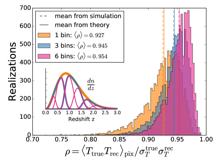
Figure 5: Histogram of $\displaystyle\rho$ values measured from 10,000 map realizations for selected binning strategies. The inset shows the un-normalized $\displaystyle dn/dz$ distributions for the sets of redshift bins considered.

We see that splitting data into redshift bins improves our ISW reconstruction, if only slightly: the correlation between the reconstructed and true map shifts by $\displaystyle\Delta\rho\lesssim 0.03$. This change is smaller than the observed scatter in $\displaystyle\rho$ and is comparable to that produced in the previous section by shifting the survey depth by $\displaystyle\Delta z=\pm 0.1$ about $\displaystyle z_{0}=0.7$. This improvement could be due to gains in three-dimensional information, or to the fact that we are now using multiple LSS maps with uncorrelated noise.

Reassured that $\displaystyle\langle\rho\rangle$ is still a reliable statistic, we compute it for all 32 possible combinations of the six bins from Fig. 4. The results are shown in Fig. 6. In this figure, the bars labeling the $\displaystyle y$-axis schematically illustrate the binning configurations, with different colors corresponding to different numbers of bins. The data points show $\displaystyle\langle\rho\rangle$ for various values of $\displaystyle\sigma_{z0}$, while the X-shaped points with error bars show the mean and standard deviations extracted from the histograms in Fig. 4.

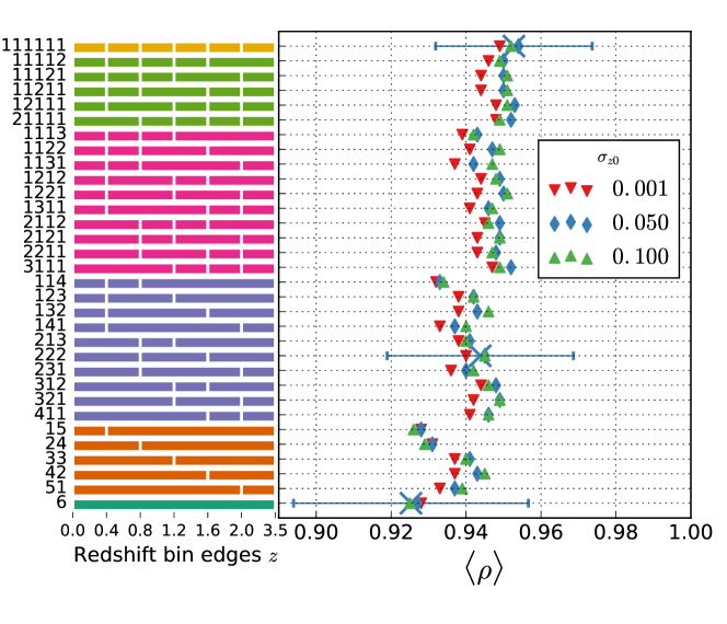
Figure 6: Theoretical expectation value for $\displaystyle\rho$ computed for different redshift binning strategies and levels of photometric-redshift uncertainties. The colored bars and corresponding numbers on the left side of the plot are schematic labels for how the galaxies are divided into redshift bins. Different colored points show the effect of different photo-$\displaystyle z$ uncertainties. The “X” points with blue horizontal errorbars show the mean and standard deviation of $\displaystyle\rho$ extracted from the histograms in Fig. 5.

We note a couple of patterns in the results. First, for a fixed number of bins, the reconstruction tends to be better if we place finer divisions at high redshift. Also, having a smaller photometric-redshift uncertainty actually slightly degrades the reconstruction rather than improving it. This implies that combining maps with redshift distributions which overlap more tend to lead to better reconstructions. This could be due a multitracer effect, in that overlap between bins means that we are sampling the same potential fluctuations with multiple source populations. However, it is also possible this is due to how our model of $\displaystyle\sigma(z)$ affects the shapes of the redshift distributions. Given the small size of these effects, one should be cautious about assigning them much physical significance.

Last, we observe a shift $\displaystyle\Delta\rho$ due to changes in binning that is smaller than what is found in the work byManzotti and Dodelson (2014) by about a factor of 3. Because their simulated DES-like survey is shallower than our fiducial survey and the relationship between $\displaystyle\Delta\rho$ and $\displaystyle\bar{\rho}$ is nonlinear (e.g., a shift from 0.98 to 0.99 is more significant than one from 0.28 to 0.29), this does not necessarily mean that our results are incompatible. As a cross-check, we performed additional simulations similar to those analyzed in Ref. Manzotti and Dodelson (2014). Our results, discussed in Appendix A, support this.

III.3 Varying $\displaystyle\ell_{\rm min}$ of reconstruction

For most of the studies presented in this paper, we reconstruct and assess the accuracy of ISW maps using all multipoles with $\displaystyle 2\leq\ell\leq 95$. This range is chosen because $\displaystyle\ell=2$ is the lowest multipole typically considered for CMB analysis and $\displaystyle\ell=95$ is the maximum multipole retaining information in NSIDE=32 Healpix maps. In this section, we study the effect of changing $\displaystyle\ell_{\rm min}$.

When we perform ISW map reconstruction, we enforce $\displaystyle\ell$-range requirements in three ways. First, when we construct the ISW estimator shown in Eq. (10), we set all $\displaystyle R_{\ell}^{i}$ not satisfying $\displaystyle\ell_{\rm min}\leq\ell\leq\ell_{\rm max}$ to be zero, so the reconstructed map contains no information from multipoles outside that range. Second, when analyzing simulations, we remove the same $\displaystyle\ell$ values from maps before computing $\displaystyle\rho$. Likewise, when we analytically compute $\displaystyle\langle\rho\rangle$ as shown in Eq. (18), we restrict the sum over multipole to $\displaystyle\ell_{\rm min}\leq\ell\leq\ell_{\rm max}$. In other words, when we show $\displaystyle\rho_{\ell\geq\ell_{\rm min}}$, we are showing the result for an ISW map reconstructed for a limited range of $\displaystyle\ell$ values, evaluated by considering only those multipoles.

The results of this analysis are shown in Fig. 7. Here we show the correlation coefficient between true and reconstructed maps $\displaystyle\rho_{[\ell\geq\ell_{\rm min}]}$ as a function of the minimum multipole used in the reconstruction. The solid line is the theoretical expectation value, while the data points with error bars show results from simulations. We find that $\displaystyle\rho$ increases with the minimum multipole out to $\displaystyle\ell_{\rm min}\sim 5$, after which it begins to very gradually decrease with $\displaystyle\ell_{\rm min}$. Increasing $\displaystyle\ell_{\rm min}$ also decreases the scatter in $\displaystyle\rho$ measured across realizations.

We interpret these trends to be the result of a competition between cosmic variance and the fact that most ISW information (power and cross-power) is at small multipoles. That is, removing the lowest few multipoles (out to $\displaystyle\ell\simeq 4$) from the analysis largely removes noise due to cosmic variance, while removing further multipoles largely removes ISW information. This has implications for efforts to reconstruct ISW maps from data; if we only care about small-angle features, it can be worth ignoring a few low-$\displaystyle\ell$ modes in order to get a more accurate reconstruction. Conversely, if we want to study how the ISW signal contributes to the CMB quadrupole and octupole, we must recognize that reconstruction quality will be necessarily less predictable.

Because cosmic variance of the ISW $\displaystyle C_{\ell}$ has a nontrivial relationship with the value and scatter of $\displaystyle\rho$, one cannot make a direct connection between $\displaystyle\ell_{\rm min}$ and how $\displaystyle f_{\rm sky}$ affects reconstruction, as is done in the ISW signal-to-noise detection studies (e.g., Ref. Douspis et al. (2008)). To understand how sky coverage affects reconstruction, one should perform simulations using the mask appropriate for a given survey. We refer the reader to Ref. Bonavera et al. (2016) for an analysis of how ISW signal reconstruction is affected by survey masks.

We also looked at the impact of varying $\displaystyle\ell_{\rm max}$ but found that the correlation coefficient $\displaystyle\rho$ is insensitive to it, and therefore do not show it.

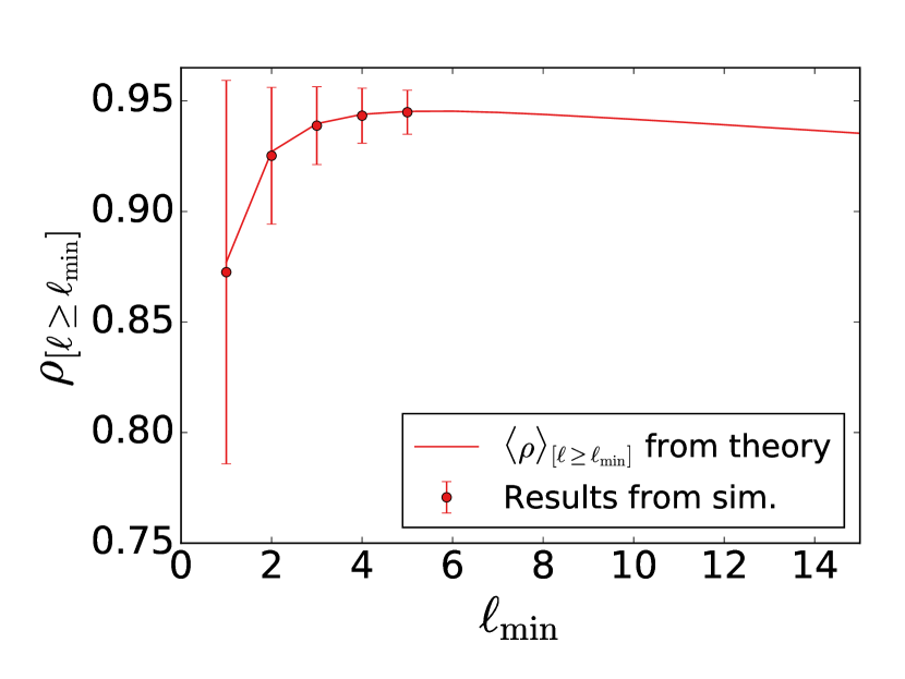
Figure 7: How filtering out angular scales with $\displaystyle\ell>\ell_{\rm min}$ affects reconstruction of ISW map. The data points show the mean and standard deviation of $\displaystyle\rho$, the correlation coefficient between true and reconstructed ISW maps, observed in 10,000 realizations, while the line shows the value of $\displaystyle\langle\rho\rangle$ computed analytically.

III.4 Varying $\displaystyle\bar{n}$

Additionally, we studied how the level of galaxy shot noise affects reconstruction. For this test, we varied the number density of sources, $\displaystyle\bar{n}$, for our fiducial survey and introduced it to both $\displaystyle C_{\ell}^{\rm true}$ and $\displaystyle C_{\ell}^{\rm model}$ according to Eq. (6). Our results are shown in Fig. 8.

We find that as long as $\displaystyle\bar{n}\gtrsim 1\,{\rm arcmin}^{-2}\approx 10^{7}\,{\rm sr}^{-1}$, shot noise will have a negligible impact on reconstruction. Note that this requirement is easily satisfied by essentially all photometric surveys (e.g., for DES or Euclid, $\displaystyle n\simeq(10-30)\,{\rm arcmin}^{-2}$). However, the quality of the reconstruction degrades rapidly for lower values of number density; once $\displaystyle\bar{n}\lesssim 10^{-3}\,{\rm arcmin}^{-2}\approx 10^{4}\,{\rm sr}^{-1}$, the reconstruction contains effectively no information about the true ISW map. Therefore, ISW reconstruction from spectroscopic galaxy surveys, as well as galaxy cluster samples, may be subject to degradations due to high shot noise.

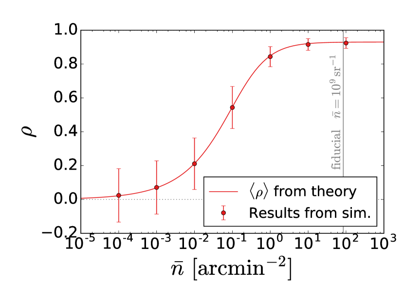
Figure 8: How changing $\displaystyle\bar{n}$ affects reconstruction of the ISW map. The datapoints show the mean and standard deviation of $\displaystyle\rho$, the correlation coefficient between true and reconstructed ISW maps, observed in 10,000 realizations. The line shows the value of $\displaystyle\langle\rho\rangle$ computed analytically.

IV Results II: The effect of survey systematics

Large-scale structure surveys are subject to a variety of systematic errors that limit the extent to which LSS tracers can be used to probe dark matter, dark energy, and primordial physics. These systematics can be astrophysical, instrumental, or theoretical in origin. Concretely, in this work, they include anything that makes $\displaystyle C_{\ell}^{\rm model}\neq C_{\ell}^{\rm true}$, which will cause the estimator given in Eq. (10) to become suboptimal. Our goal is to study these LSS systematics generally, without requiring specific information about a LSS survey (e.g., wavelengths at which it observes the sky). We do this by considering two broad classes of LSS systematics:

1. Mismodeling of the distribution of LSS sources along the line of sight.

2. Direction-dependent calibration errors.

Our studies will give us some insight into which, and how much, systematics need to be controlled if one wishes to use LSS data to reconstruct a map of the ISW signal.

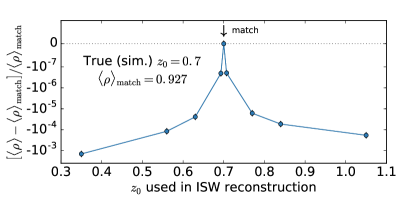
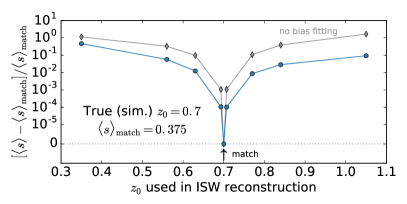
Figure 9: Impact of mismodeling survey depth on the expected correlation between the true and reconstructed ISW maps $\displaystyle\langle\rho\rangle$ (left panel) and the ratio of the average size of residuals to that of ISW map features $\displaystyle\langle s\rangle$ (right panel). The true value of the parameter $\displaystyle z_{0}$, which controls the depth of the survey, is fixed at 0.7, while the values used for reconstruction are shown on the $\displaystyle x$-axis. The blue circular points show results from our standard reconstruction pipeline, while the gray diamond-shaped points (directly behind the blue points in the $\displaystyle\rho$ plot) show results when we skip the $\displaystyle\bar{b}$-fitting step. The $\displaystyle y$-axis is linear within one tick mark of zero; otherwise, it has logarithmic scaling.

IV.1 Modeling redshift distribution of sources

In the context of ISW map reconstruction, it would be reasonable to guess that accurate knowledge of galaxy redshifts is important for our ability to correctly associate the observed number density fluctuations on the sky with the three-dimensional gravitational potential fluctuations which source the ISW signal. Uncertainties about redshift distributions are a pervasive class of systematics affecting LSS surveys, which have already been studied by numerous authors (e.g., Refs. Ma et al. (2005); Bernstein and Huterer (2010)) in the context of cosmological parameter measurements from photometric surveys. Here we study how redshift modeling errors affect the ISW reconstruction accuracy.

For the purposes of this discussion, we define redshift uncertainties broadly as anything that makes the galaxy window function (Eq. (5)) used in our ISW estimator different from that which describes the the true line-of-sight distribution of objects we observe on the sky. We study three specific cases of this: the mismodeling of a survey’s median redshift, redshift-dependent bias, and the fraction of catastrophic photometric-redshift errors. In each case, we identify a parameter which controls the survey characteristic in question. Then, choosing a true (simulation) value for that parameter, we perform reconstructions using several mismodeled values as input to the ISW estimator. This allows us to and look at how the theoretical expectation values of our quality statistics respond relative the best, correctly modeled case.

Let us place these shifts in context by referring to previous sections. In an ideal scenario with no systematic errors, changing the survey depth parameter (see Section III.1) from the fiducial $\displaystyle z_{0}=0.7$ to 0.6 (0.8) causes $\displaystyle\langle\rho\rangle$ to change by 3% (1.5%) and $\displaystyle\langle s\rangle$ by 20% (10%). Also, splitting our fiducial survey into $\displaystyle 6$ redshift bins (in Sec. III.2) improves $\displaystyle\langle\rho\rangle$ by 3% relative to the one-bin case.

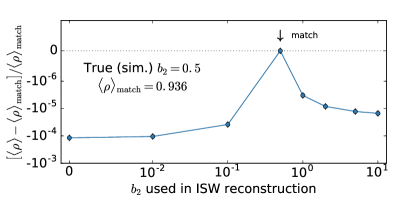
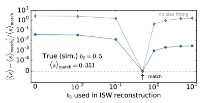
Figure 10: Impact of mismodeling redshift-dependent bias on the expected correlation between the true and reconstructed ISW maps $\displaystyle\langle\rho\rangle$ (left panel), and the typical size of residuals relative to that of ISW map features $\displaystyle\langle s\rangle$ (right panel). The bias is modeled as $\displaystyle b(z)=1+b_{2}(1+z)^{2}$ with the true value fixed at $\displaystyle b_{2}=0.5$ and the values used in the ISW estimator shown on the $\displaystyle x$-axis. Both axes have logarithmic scaling except in regions within one tick mark of zero, where they are linear. The blue circular points show results from our standard reconstruction pipeline, while the gray diamond-shaped points (directly behind the blue points in the $\displaystyle\rho$ plot) show results when we skip the $\displaystyle\bar{b}$-fitting step.

IV.1.1 Median redshift

We begin by studying how reconstruction accuracy responds when we construct the ISW estimator using the wrong median LSS source redshift. Though the parameter $\displaystyle z_{0}$ in the $\displaystyle dn/dz$ distribution given in Eq. (9) is lower than $\displaystyle z_{\rm median}$, raising or lowering it will have a similar effect as shifting the median of the distribution. We thus use $\displaystyle z_{0}$ as a proxy for median redshift. We compute $\displaystyle C_{\ell}^{\rm true}$ with $\displaystyle z_{0}$ fixed at its fiducial value of 0.7, and vary the $\displaystyle z_{0}$ values used to compute $\displaystyle C_{\ell}^{\rm model}$.

Figure 9 shows the fractional change in our reconstruction statistics when the value of $\displaystyle z_{0}$ used for reconstruction is shifted from its true value by $\displaystyle\pm 1\%$, $\displaystyle\pm 10\%$, $\displaystyle\pm 20\%$, $\displaystyle\pm 30\%$, and $\displaystyle\pm 50\%$. We see that even for large shifts in $\displaystyle z_{0}$ (with correspondingly dramatic mismatches between the true and model $\displaystyle dn/dz$) the fractional change in $\displaystyle\rho$ is less than $\displaystyle\mathcal{O}(10^{-3})$. The effect on $\displaystyle s$ is also small; for all but the most extreme points, the fractional change in the size of residuals $\displaystyle\langle s\rangle$ is less than 10%.

To understand this lack of sensitivity of $\displaystyle z_{0}$, it is instructive to note that varying $\displaystyle z_{0}$ changes $\displaystyle C_{\ell}$ by a nearly scale-independent amplitude. (See Appendix B for plots demonstrating this.) As we observed in Sec. II.5, $\displaystyle\rho$, the correlation coefficient between true and reconstructed ISW maps, is insensitive to overall shifts in the the map amplitude. The fact that it does not respond strongly to these changes in $\displaystyle z_{0}$ is thus not surprising. The statistic $\displaystyle\langle s\rangle$, which measures the size of residuals, is sensitive to changes in amplitude, however. The fact that it also displays small fractional changes illustrates the importance of the bias-fitting procedure described in Sec. II.4. Because the effects of mismodeling $\displaystyle z_{0}$ are degenerate with shifts in constant bias, fitting for $\displaystyle\bar{b}$ protects our reconstruction against this kind of systematic.

For comparison, we compute $\displaystyle\langle\rho\rangle$ and $\displaystyle\langle s\rangle$ while neglecting the bias-fitting step and show the results as gray points in Fig. 9. We see no change in the $\displaystyle\rho$ plot (the gray points are directly behind the blue ones), reflecting the fact that $\displaystyle\rho$ is insensitive to constant multipliers. In the $\displaystyle s$ plot, we see that the bias-fitting procedure suppresses the size of the reconstruction errors by about an order of magnitude.

To summarize, we find that the quality of the ISW reconstruction is much less dependent on our knowledge of the survey’s median redshift than naively expected. The median redshift mostly changes the normalization of the $\displaystyle C_{\ell}$, but so does the galaxy bias (which, recall, is to a good approximation scale independent at the large scales we are studying). By fitting for the bias parameter in the angular power spectrum—something that is typically done in LSS surveys regardless of their application—one effectively also fits for $\displaystyle z_{0}$. As a result, the combination of the galaxy bias and survey depth that enters the amplitude of the $\displaystyle C_{\ell}$ is fit to the correct value.

IV.1.2 Redshift-dependent bias

Here, we study what happens if the redshift dependence of the galaxy bias is modeled incorrectly. Using the functional forms given in Ref. Ade et al. (2015a) for guidance, we parametrize the redshift dependence of the bias via

$$b(z)=b_{0}(1+b_{2}(1+z)^{2}).$$ (27)

For this study, we set $\displaystyle b_{0}=1$ and vary $\displaystyle b_{2}$, noting that Ref Ade et al. (2015a) uses $\displaystyle b_{2}\sim 0.5$ for sources in NVSS and WISE-AGN.

In the expression for $\displaystyle C_{\ell}$, $\displaystyle b(z)$ appears inside the same integrand as $\displaystyle dn/dz$, so changes to $\displaystyle b(z)$ have an effect similar to altering the LSS source redshift distribution. The results here, shown in Fig. 10, are thus similar to what was seen in the previous section. Increasing $\displaystyle b_{2}$ mostly just increases the overall amplitude of the galaxy $\displaystyle C_{\ell}$’s, so the reconstruction is not very sensitive to $\displaystyle b_{2}$ once we fit for $\displaystyle\bar{b}$. For example, if the true value of $\displaystyle b_{2}$ is 0.5 and we reconstruct the ISW signal assuming no redshift dependence ($\displaystyle b_{2}=0$), the fractional change in $\displaystyle\langle\rho\rangle$ is $\displaystyle\mathcal{O}(10^{-4})$ and the fractional change in $\displaystyle\langle s\rangle$ is $\displaystyle\mathcal{O}(10^{-2})$. The reason the $\displaystyle\bar{b}$-fitting step has a larger effect here than in the $\displaystyle z_{0}$ study above is probably because the normalization requirements of $\displaystyle dn/dz$ somewhat limit the size of $\displaystyle C_{\ell}$ amplitude shifts, whereas $\displaystyle b(z)$ has no such normalization scaling.

IV.1.3 Catastrophic photo-z error rate

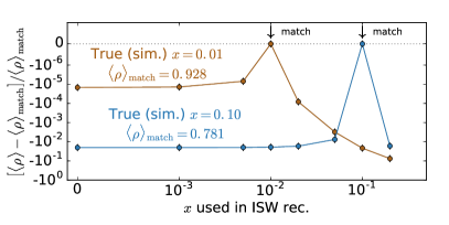
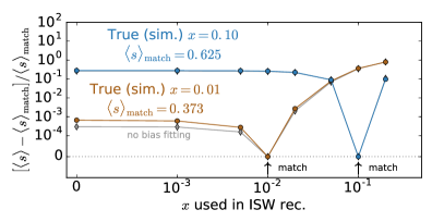
Figure 11: Impact of mismodeling the fraction $\displaystyle x$ of galaxies subject to catastrophic photo-$\displaystyle z$ errors on the expected correlation between the true and reconstructed ISW maps $\displaystyle\langle\rho\rangle$ (left panel), and the typical size of residuals relative to that of ISW map features $\displaystyle\langle s\rangle$ (right panel). Both axes have logarithmic scaling except in regions within one tick mark of zero, where they are linear. The blue and brown circular points show results from our standard reconstruction pipeline when the true value of $\displaystyle x$ is 0.1 and 0.01 respectively. The gray diamond-shaped points (directly behind the other points in the $\displaystyle\rho$ plot and the blue points in the $\displaystyle s$ plot) show results when we skip the $\displaystyle bar{b}$-fitting step.

Galaxies in photometric-redshift surveys are also subject to so-called catastrophic photometric-redshift errors—cases where the true redshift is misestimated by a significant amount Bernstein and Huterer (2010); Hearin et al. (2010). This is a distinct effect from the photo-$\displaystyle z$ uncertainty modeled in the binning tests in Sec. III.2, which causes a redshift bin selected using sharp cuts in photo-$\displaystyle z$ to occupy a smoothed distribution in the spectroscopic redshift. Rather, for galaxies suffering catastrophic photo-$\displaystyle z$ errors, the photometric-redshift finding algorithms have failed, and the spectroscopic redshift corresponding to a given photo-$\displaystyle z$ is effectively randomized. The reasons for this are not fully understood, but, like the conventional photo-$\displaystyle z$ error case, the rate and outcome of catastrophic errors depend strongly on the number of photometric filters and their relation to the spectral features that carry principal information about the redshift.

In the absence of detailed, survey-specific information about the photometric pipeline, we model catastrophic redshift errors by randomly assigning the true redshift of a fraction $\displaystyle x$ of the galaxies in our sample (e.g., $\displaystyle x=0.01$ means that one in a hundred galaxies has a catastrophic photo-$\displaystyle z$ error). We implement this by modifying the redshift distribution of each bin $\displaystyle i$ to

$$\frac{d\tilde{n}^{i}}{dz}=(1-x)\frac{dn^{i}}{dz}+x\bar{n}^{i}\left[\Theta(z-z_{\rm min})-\Theta(z_{\rm max}-z)\right],$$ (28)

where $\displaystyle x$ is the fraction of galaxies suffering catastrophic errors, $\displaystyle dn^{i}/dz$ is the redshift distribution of bin $\displaystyle i$ without catastrophic errors, and $\displaystyle\Theta$ is the Heaviside step function. The added term on the right models the fact that, of the $\displaystyle\bar{n}^{i}$ galaxies assigned to that photometric-redshift bin, $\displaystyle x\bar{n}^{i}$ of them have spectroscopic redshifts which are randomized across the full range of the survey. For our analysis, we choose the range of these randomized redshifts to be $\displaystyle z\in[z_{\rm min},z_{\rm max}]=[0.01,2.5]$. In practice, we significantly smooth the edges of the step function to avoid numerical artifacts in our $\displaystyle C_{\ell}$ calculations.

For this study, we use two different true (simulation) catastrophic photo-$\displaystyle z$ fractions: $\displaystyle x=0.01$ and 0.1; these values roughly bracket the currently achieved levels of catastrophic outliers in current surveys (e.g., CFHTLens Hildebrandt et al. (2012)). Figure 11 shows the fractional change in $\displaystyle\langle\rho\rangle$ and $\displaystyle\langle s\rangle$ when the ISW estimator is constructed assuming various values of $\displaystyle x$, with true $\displaystyle x=0.01$ and $\displaystyle x=0.1$ shown in blue and brown lines, respectively.

Our results show us two things. First, though mismodeling $\displaystyle x$ results in more significant changes than what was seen for the survey depth and redshift-dependent bias, the shifts are still relatively small; in the worst-case scenarios, $\displaystyle\langle\rho\rangle$ shifts by less than 10% and $\displaystyle\langle s\rangle$ shifts by about 20%. Second, the constant-bias-fitting step of our pipeline does not provide protection against mismodeled catastrophic photo-$\displaystyle z$ error rates. This is because the $\displaystyle dn/dz$ modification in Eq. (28) alters $\displaystyle C_{\ell}$ in a scale-dependent way, as can be seen in the plots in Appendix B.

To check whether catastrophic photo-$\displaystyle z$ errors are more damaging when LSS data are binned in redshift, we ran a similar analysis for a case where the fiducial $\displaystyle dn/dz$ was split into three redshift bins. We observed fractional changes in the quality statistics similar to those seen for the one-bin case, so we conclude that our results are roughly independent of the binning strategy.

In summary, we find that properly modeling a survey’s catastrophic photo-$\displaystyle z$ error fraction is more important for preserving ISW reconstruction quality than either its depth or redshift-dependent bias but that, overall, reconstruction is relatively robust against these kinds of errors.

IV.2 Photometric calibration errors

Photometric calibration errors are a very general class of systematics that cause the magnitude limit of a survey to vary across the sky. This introduces direction-dependent number density variations which do not correspond to fluctuations in physical matter density, thus biasing the observed galaxy power spectrum. Examples of photometric calibration errors include atmospheric blurring, unaccounted-for Galactic dust, and imperfect star-galaxy separation, among other things. A number of recent LSS observations have found a significant excess of power at large scales (Pullen and Hirata, 2013; Ho et al., 2012, 2013; Agarwal et al., 2014a; Giannantonio et al., 2014; Agarwal et al., 2014b), suggesting the presence of this kind of error.

We adopt a parametrization of calibration errors from Huterer et al. (2013), who presented a systematic study of the effects of calibration errors and requirements on their control for cosmological parameter estimates. See also Refs. (Leistedt et al., 2013; Leistedt and Peiris, 2014; Shafer and Huterer, 2015) for other approaches. We model photometric calibration errors in terms of a calibration error field $\displaystyle c({\bf\hat{n}})$ which modifies the observed number density $\displaystyle N^{\rm obs}$ via

$$N^{\rm obs}({\bf\hat{n}})=\left(1+c({\bf\hat{n}})\right)N({\bf\hat{n}}).$$ (29)

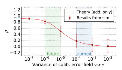
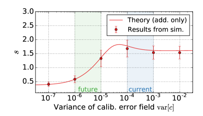
Figure 12: The effect of photometric calibration errors on reconstruction quality. We show results for the correlation coefficient between true and reconstructed ISW maps (left panel) and for the typical size of map residuals relative to the variance of the true ISW map (right panel). The lines show the expectation from theory, considering only additive contributions from calibration errors, while the data points show the mean and standard deviation from 10,000 simulated map realizations. The shaded regions show the current and projected levels of control over residual calibration errors discussed in Sec. IV.2.1.

This kind of direction-dependent “screen” is straightforward to implement on the level of maps but complicates the process of computing the theoretical expectation value for our statistics, $\displaystyle\langle\rho\rangle$ and $\displaystyle\langle s\rangle$. Because multiplicative effects introduce mixing between spherical components of the galaxy maps, there is a nontrivial relationship between the power spectra for the true galaxy distribution, the observed galaxy distribution, and the calibration error field $\displaystyle c({\bf\hat{n}})$. (See, for example, Refs. Huterer et al. (2013); Shafer and Huterer (2015).) To make calculations tractable, we use the fact that calibration error effects will be dominated by additive contributions at large angular scales and estimate

$$\left[C_{\ell}^{XY}\right]^{\rm obs}\approx\frac{C_{\ell}^{XY}+C^{{\rm cal}XY}_{\ell}-\delta_{\ell 0}c^{X}_{00}c^{Y}_{00}}{(1+c^{X}_{00}/\sqrt{4\pi})(1+c^{Y}_{00}/\sqrt{4\pi})}.$$ (30)

Here, $\displaystyle C^{{\rm cal}XY}_{\ell}$ is the cross-power between calibration error fields affecting maps $\displaystyle X$ and $\displaystyle Y$. The $\displaystyle c^{X}_{00}\equiv\left(C^{{\rm cal}X}_{\ell=0}\right)^{1/2}$ terms are their monopoles, which contribute by shifting $\displaystyle\bar{n}^{X}$. We derive this expression in Appendix C.

Note that this modification is only applied to $\displaystyle C_{\ell}^{\rm true}$. We wish to study the impact of uncorrected calibration errors, so we will always (when analyzing simulations or calculating quality statistic expectation values) compute $\displaystyle C_{\ell}^{\rm model}$ without including calibration error effects.

For this analysis, we adopt a functional form for the calibration error field power spectrum,

$$C_{\ell}^{\rm cal}=\begin{cases}\alpha^{\rm cal}\exp{\left[-(\ell/10)^{2}\right]}&\text{ if }\ell\leq 30\\ 0&\text{otherwise}\end{cases}$$ (31)

where $\displaystyle\alpha^{\rm cal}$ is a normalization constant set to fix the variance of $\displaystyle c({\bf\hat{n}})$ to a desired value. The variance is given by

$${\rm var}\left[c\right]\equiv\langle c^{2}({\bf\hat{n}})\rangle=(4\pi)^{-1}\sum_{\ell}(2\ell+1)C_{\ell}^{\rm cal}.$$ (32)

The form of Eq. (31) is inspired by power spectrum estimates for maps of dust extinction corrections and magnitude limit variations in existing surveys. (See Figs. 5 and 6 in Ref. Huterer et al. (2013)) Using this power spectrum, we generate independent Gaussian realizations of $\displaystyle c({\bf\hat{n}})$ which are then combined with our simulated galaxy maps according to Eq. (29). These postprocessed maps are used as input for ISW reconstruction.

IV.2.1 Context: Current and future levels of calibration error

To put our results in context, it is useful to identify what values of variance in the calibration field $\displaystyle{\rm var}[c]$ are expected from current and future surveys. Here we emphasize that we are talking about residual calibration errors—that is, calibration errors which are not properly corrected for and thus can cause biases in cosmological inferences.

Above, we defined these errors in terms of variations in the number of observed galaxies. To relate this to variations in a survey’s limiting magnitude, we must multiply the magnitude variations by a factor of $\displaystyle\ln(10)s(z)$, where $\displaystyle s(z)\equiv\left.d\log_{10}N/dm\right|_{\rm m_{\rm lim}}$ is the survey-dependent faint-end slope of the luminosity function; see Eq. (30) in Ref. Huterer et al. (2013). We adopt $\displaystyle s(z)\simeq 0.3$ estimated from the simulations of Ref. Jouvel et al. (2009), assuming a median galaxy redshift $\displaystyle z\sim 0.75$. This means that the conversion factor is $\displaystyle\ln(10)s(z)\sim 1$, and variance in calibration is roughly equal to that in the limiting magnitude, $\displaystyle c({\bf\hat{n}})\equiv(\delta N/N)({\bf\hat{n}})\simeq(\delta m)_{\rm lim}$.

With these assumptions, the smallest currently achievable variance of the calibration error $\displaystyle c({\bf\hat{n}})$ is of order $\displaystyle{\rm var}[c]\sim 10^{-3}$ (e.g., Fig. 14 in Ref. Leistedt et al. (2013)). For example, residual limiting magnitude variations in the SDSS DR8 survey are at the level of $\displaystyle 0.03$ mag Rykoff et al. (2015), again implying that $\displaystyle{\rm var}[c]\simeq 10^{-3}$. Note that, while the impressive SDSS “uber-calibration” to 1% Padmanabhan et al. (2008) would imply an order of magnitude smaller variance, this might be difficult to achieve in practice because there are sources of calibration error that come from the analysis of the survey and are not addressed in the original survey calibration. We show the current levels of residual calibration errors value as a blue vertical band in Fig. 12, spanning a range between the optimistic level associated with the SDSS uber calibration to the more conservative $\displaystyle{\rm var}[c]=10^{-3}$.

In the same figure, we also show the future control of calibration errors required to ensure that they do not contribute appreciably to cosmological parameter errors—e.g., those in dark energy and primordial non-Gaussianity. This range, forecasted assuming final DES data and adopted from Ref. Huterer et al. (2013), is shown as a green band spanning $\displaystyle{\rm var}[c]\sim 10^{-6}$–$\displaystyle 10^{-5}$. The lower bound is set by the requirement that the bias to cosmological parameter estimates be smaller than their projected errors, while $\displaystyle 10^{-5}$ is chosen as an intermediate value between that and $\displaystyle{\rm var}[c]=10^{-4}$, which introduces unacceptable levels of bias. (See Fig. 4 of Ref. Huterer et al. (2013).) These should be viewed as only rough projections, as the precise requirements depend on the faint-end slope $\displaystyle s(z)$ of the source luminosity function, the cosmological parameters in question, and the shape of the calibration field’s power spectrum $\displaystyle C_{\ell}^{\rm cal}$.

IV.2.2 Results for ISW reconstruction

We find that even small levels of calibration error can have a significant impact on ISW reconstruction quality. Figure 12 shows how the correlation between true and reconstructed maps, $\displaystyle\rho$, and the reconstructed map residuals, $\displaystyle s$, respond to different levels of calibration error.

Reconstruction quality starts to degrade when $\displaystyle{\rm var}[c]\sim 10^{-6}$, which roughly corresponds to the same 0.1% magnitude calibration required to achieve cosmic-variance-limited ISW detection Afshordi (2004). At this level, we see $\displaystyle\rho$ begin to move away from its best-case (no calibration error) value and the $\displaystyle s$ plot shows that residuals are comparable in amplitude to fluctuations due the true ISW signal.

Once the calibration error power starts to dominate over the galaxy autopower, occurring around $\displaystyle{\rm var}[c]\sim 10^{-4}$, the reconstruction contains little information about the true ISW signal. Here, the scatter in $\displaystyle\rho$ overlaps with zero and we see that the reconstructed map residuals approach a constant value. See Appendix D for an explanation of why we expect this to occur.

Comparing these numbers to the shaded bands, we see that, with current levels of calibration error control, we have little hope of accurately reconstructing the ISW signal with galaxy survey data alone. Encouragingly, though, the levels of control required to obtained unbiased cosmological parameter estimates from next-generation surveys Huterer et al. (2013) are precisely the levels needed for accurate ISW reconstruction.

We note that the additive-error-only theory calculations show good agreement with our results from simulations, and so can be useful as a computationally efficient indicator of when calibration errors become important. In light of this, we also computed $\displaystyle\langle\rho\rangle$ and $\displaystyle\langle s\rangle$ using a power law spectrum, $\displaystyle C_{\ell}^{\rm cal}\propto\ell^{-2}$, in order to check how sensitive our results are to the shape of the calibration error field’s power spectrum. This more sharply peaked spectrum caused reconstruction quality to start degrading at a slightly smaller $\displaystyle{\rm var}[c]$ compared to the Gaussian model, but otherwise showed similar results. This can likely be explained by the fact that the power law $\displaystyle C_{\ell}^{\rm cal}$ reaches higher values at low $\displaystyle\ell$ for a given field variance, which means it can start dominating over true galaxy power at those multipoles earlier.

IV.2.3 Mitigation by raising $\displaystyle\ell_{\rm min}$

Because calibration error fields tend to have the most power on large scales, we looked at whether raising $\displaystyle\ell_{\rm min}$ can mitigate their impact. Our results, shown in Fig. 13, show that raising $\displaystyle\ell_{\rm min}$ from 2 to 3 or 5 causes the error bars denoting the scatter in $\displaystyle\rho$ to cross zero at a higher value of $\displaystyle{\rm var}[c]$. However, this effect is small, and we conclude that raising $\displaystyle\ell_{\rm min}$ provides only limited protection against calibration errors.

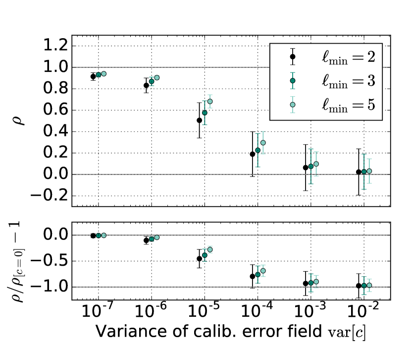
Figure 13: Exploration of whether raising $\displaystyle\ell_{\rm min}$ can mitigate the impact of photometric calibration errors on ISW signal reconstruction. The top panel shows the mean and standard deviation of $\displaystyle\rho$, the correlation between the true and reconstructed ISW maps, measured from 10,000 simulations. The bottom panel shows the fractional change in $\displaystyle\rho$ relative to the case with no calibration errors. Points for different values of $\displaystyle\ell_{\rm min}$ are staggered so that the errors bars are legible; each cluster of three points shares the same value of $\displaystyle{\rm var}\left[c\right]$.

V Implications for cosmic alignments

Over the past 15 years, as the full-sky CMB maps provided by the WMAP and Planck experiments became available, increasing evidence has been found for anomalies at large angular scales. In particular, angular correlations at scales above 60 deg on the sky seem to be missing, while the the quadrupole and octupole moment of the CMB anisotropy are aligned both mutually and with the geometry and the direction of motion of Solar System. The origin for the anomalies is not well understood at this time; they could be caused by astrophysical systematic errors or foregrounds or cosmological causes (like departures from simple inflationary scenarios), or they could be a statistical fluctuation, albeit a very unlikely one. The anomalies have most recently been reviewed in Ref. Schwarz et al. (2015).

Some authors Francis and Peacock (2010); Rassat et al. (2013) have commented on the fact that current efforts to “peel off” the ISW contribution from the CMB maps indicate that the significance of some CMB anomalies is “significantly reduced” once the ISW contribution is subtracted. If true, this statement implies that the observed anomalies are either due to features in the ISW map or caused by an accidental alignment of the early- and late-time CMB anisotropy Copi et al. (2015). In any case, statements on how the primordial and late CMB combine to produce the anomalies clearly depend on the fidelity of the reconstructed ISW contribution to the CMB, which is the subject of our work.

Our goal here is not to carry out a full investigation of the ISW map reconstruction’s effect on the anomalies’ significance. Instead, we would like to simply build intuition on how much imperfect reconstruction affects inferences about the anomalies.

To that end, we pose the following question: if we assume for the moment that an ISW map reconstructed using available LSS data happens to show a significant quadrupole-octupole alignment, what is the likelihood that the true ISW map is actually aligned? Note that we in no way imply that the ISW-only alignment scenario is a favored model for the observed CMB anomalies. We simply want to study how robust certain properties of the ISW map, particularly the phase structure of the anisotropies in the map, are to the reconstruction process.

To study the alignments, we adopt the (normalized) angular momentum dispersion maximized over directions on the sky, defined as (de Oliveira-Costa et al., 2004; Copi et al., 2006)

$$(\Delta L)^{2}_{\rm 2+3,true}\equiv\max_{{\bf\hat{n}}}\left(\frac{\sum_{m=-\ell}^{\ell}m^{2}\,|a_{\ell m}({\bf\hat{n}})|^{2}}{\ell^{2}\sum_{m=-\ell}^{\ell}\,|a_{\ell m}({\bf\hat{n}})|^{2}}\right)$$ (33)

where $\displaystyle a_{\ell m}({\bf\hat{n}})$ are expansion coefficients of the map in a coordinate system where the $\displaystyle z$-axis is in the $\displaystyle{\bf\hat{n}}$ direction. Hence, the maximization is performed over all directions $\displaystyle{\bf\hat{n}}$; note that only the numerator of the expression in angular parentheses depends on the direction, and see Sec. 5.6 of Ref. Copi et al. (2006) for the algorithm to efficiently compute the maximization. Intuitively, high values of the angular momentum indicate significant planarity of the $\displaystyle\ell=2$ and $\displaystyle\ell=3$ modes as well as their mutual alignment.

We set up the following pipeline:

• Start with $\displaystyle 10,000$ random realizations of the true ISW map and the corresponding LSS maps (so that each LSS map contains gravitational potential field that produces the corresponding ISW map).

• For each true ISW map, measure the angular momentum dispersion $\displaystyle(\Delta L)^{2}_{\rm 2+3,true}$ defined in Eq. (33).

• Reconstruct each map assuming a fiducial LSS survey and repeat the calculation to get a set of $\displaystyle(\Delta L)^{2}_{\rm 2+3,rec}$.

• Make a scatter plot of $\displaystyle(\Delta L)^{2}_{\rm 2+3,rec}$ vs $\displaystyle(\Delta L)^{2}_{\rm 2+3,true}$, which will show how much and in which direction reconstruction biases the alignment information.

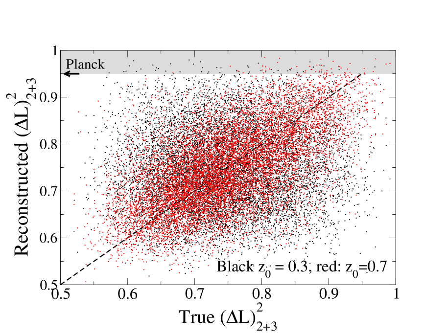
Figure 14: The relationship between the true ($\displaystyle x$-axis) and reconstructed ($\displaystyle y$-axis) angular momentum dispersion $\displaystyle(\Delta L)^{2}_{\rm 2+3}$, defined in the text, for the combined quadrupole and octupole in 10,000 randomly generated ISW maps. Results are shown for two alternate survey depths: our fiducial LSS survey with $\displaystyle z_{0}=0.7$ (red points) and $\displaystyle z_{0}=0.3$ (black points), which have correlation coefficients 0.58 and 0.11 respectively. The gray region denotes $\displaystyle(\Delta L)^{2}_{\rm 2+3}$ as high or higher than measured in WMAP and Planck CMB maps, while the diagonal line is where the true and reconstructed values match. See the text for details.

The results are summarized in Fig. 14. There we show how the inferred angular momentum dispersion of the combined quadrupole and octupole is affected by reconstruction for 10,000 randomly generated ISW maps. The $\displaystyle x$-axis shows the value for the is the true ISW map, while the $\displaystyle y$-axis shows values reconstructed from our fiducial LSS survey at two alternate depths, $\displaystyle z_{0}=0.7$ (red points) and 0.3 (black points). We find that the true and reconstructed angular momentum dispersions are not very correlated, having a correlation coefficient of only 0.58 for $\displaystyle z_{0}=0.7$ and 0.11 for $\displaystyle z_{0}=0.3$.

We also denote the value for the angular momentum dispersion of the WMAP/Planck full map, which includes both primordial and late-time ISW contributions, at $\displaystyle(\Delta L)^{2}_{\rm 2+3}\simeq 0.95$. (The precise value varies slightly depending on the map. Copi et al. (2006); Schwarz et al. (2015)) Of the $\displaystyle z_{0}=0.7$ (0.3) reconstructed maps which have $\displaystyle(\Delta L)^{2}_{\rm 2+3}$ as high as or higher than the WMAP and Planck CMB maps (points falling in the shaded gray region), only 10% (2%) have corresponding true maps which satisfy the same high angular momentum dispersion criterion.

Investigating the implications of the ISW reconstruction on the inferences about the alignments of primordial-only and ISW-only maps in depth is beyond the scope of this paper. Nevertheless, our simple test indicates that at least the quadrupole-octupole alignment in the ISW-only maps is not very robust under ISW reconstruction using realistic LSS maps, even without taking into account calibration and other systematic errors.

VI Conclusion

In this work we use simulated ISW and LSS maps to study the accuracy of ISW signal reconstructions performed using LSS data as input. In particular, we study how systematics associated with galaxy surveys affect the ISW map reconstruction. We measure reconstruction accuracy using two quality statistics: $\displaystyle\rho$, the correlation coefficient between the true and reconstructed ISW maps, and $\displaystyle s$, the rms error in the reconstructed map relative to the rms of true ISW map features.

In the absence of systematics, we find that increasing survey depth improves these statistics (brings $\displaystyle\rho$ closer to 1 and lowers $\displaystyle s$), though the shifts in their average values are small compared to their scatter. Similarly, splitting the survey data into redshift bins leads to moderate improvement. The reconstruction quality improvement due to increasing survey depth by $\displaystyle\Delta z=0.1$ is comparable to that gained by splitting into three redshift bins: both lead to improvement $\displaystyle\Delta\bar{\rho}\sim 0.02$, or $\displaystyle\Delta\bar{\rho}/\bar{\rho}\sim 2\%$. We also find that reconstruction can be slightly improved if we are willing to neglect the reconstruction of very low-$\displaystyle\ell$ multipoles; increasing our fiducial $\displaystyle\ell_{\rm min}=2$ to 5 results in $\displaystyle\Delta\bar{\rho}\sim 0.01$ and a reduction in the scatter of $\displaystyle\rho$ by about a factor of 2. Last, we find that galaxy shot noise has a negligible impact as long as $\displaystyle\bar{n}\gtrsim 1\,{\rm arcmin}^{-2}\approx 10^{7}\,{\rm sr}^{-1}$. These results provided a baseline comparison for our studies of systematics.

The first class of systematics we study are those associated with mismodeling the line-of-sight distribution of LSS sources. By examining what happens to reconstruction quality when different galaxy window functions are used for the ISW-estimator input $\displaystyle C_{\ell}^{\rm model}$ than for the simulation-generating $\displaystyle C_{\ell}^{\rm true}$, we find that ISW signal reconstruction is robust against these kinds of errors. We study the mismodeling of survey depth and redshift-dependent bias and find that fractional shifts in $\displaystyle\langle\rho\rangle$ are less than $\displaystyle\mathcal{O}(10^{-4})$ for all but the most extreme cases. Inaccurately estimating the fraction of catastrophic photo-$\displaystyle z$ errors results in a larger shift, which depends on the true fraction, but at worst this degrades $\displaystyle\langle\rho\rangle$ by about a percent. Reconstruction quality is likely to be similarly insensitive to other direction-independent modeling uncertainties; for example, the choice of cosmological parameter values and maybe models of modified gravity.

The fact that we fit data for a constant galaxy bias is the key to this robustness. This is because the modeling errors discussed above change the galaxy spectrum by a mostly scale-independent amplitude which is degenerate with a shift in constant bias $\displaystyle\bar{b}$. Thus, the more a given systematic changes the shape (rather than amplitude) of galaxy $\displaystyle C_{\ell}$, the more of an impact it will have on ISW signal reconstruction.

We find that photometric calibration errors are by far the most important systematic to control if one wants to construct a map of the ISW signal from LSS data. For the reconstructed ISW map to contain accurate information about the true ISW signal, calibration-based variations in number density must be controlled so that the calibration error field $\displaystyle c$, defined via $\displaystyle N^{\rm obs}({\bf\hat{n}})=(1+c({\bf\hat{n}}))N({\bf\hat{n}})$, has a variance less than $\displaystyle 10^{-4}$. Even at that level, which is optimistic for current surveys, the reconstruction quality is significantly degraded compared to the case with no systematics. For the model we studied, in order to keep that degradation smaller than $\displaystyle\mathcal{O}(10\%)$, calibration errors must be controlled so that $\displaystyle{\rm var}[c]\lesssim 10^{-6}$. This is a similar level to what is required to avoid biasing cosmological parameter estimates made with future survey data. Prospects for mitigation of these effects by neglecting low $\displaystyle\ell$ multipoles are limited.

We also briefly explore the viability of using reconstructed ISW maps to comment on the significance and origins of observed large-angle CMB anomalies. We do this by comparing the level of alignment, parametrized in terms of angular momentum dispersion, observed for the $\displaystyle\ell=2,3$ modes of true and reconstructed ISW maps. We find that, even in the absence of systematics, the amount of alignment was only weakly correlated between these maps. For example, the values of true and reconstructed angular momentum dispersion had a correlation coefficient of only 0.58 for our fiducial survey. Therefore, recovering precise alignments of structures in the ISW map, using only LSS data as input, seems like a very challenging prospect.

These results have implications for current and future attempts to reconstruct the ISW signal. Most significantly, they tell us that understanding the level and properties of residual calibration errors in LSS maps is vital to assessing the accuracy of reconstructions made using those maps as input. Given the current levels of calibration error control, at face value our results would seem to imply that reconstruction using existing data is hopeless. Thus, a productive avenue for future work would be to modify the ISW reconstruction pipeline to make it more robust against calibration errors, by including them in the ISW estimator’s noise modeling or by some other method. Since the presence of uncorrected calibration errors will cause one to underestimate galaxy-galaxy noise, it would also be worth turning a critical eye toward how calibration uncertainties affect the evaluation of ISW detections’ signal to noise.

We note that using multiple cross-correlated LSS data sets—which map the same potential fluctuations but are presumably subject to different systematics—will mitigate the impact of calibration errors, as will combining LSS maps with CMB temperature and polarization data. The results of the binning test in Sec. III.2 provide provisionary evidence for this, though for that study it is not possible to disentangle the effects of noise mitigation from those of adding tomographic information. An interesting extension to this work would thus be to explore in more detail whether and to what extent using multiple LSS maps protects ISW reconstruction against calibration errors. Studying the combination of multiple surveys introduces a number of new questions: one might study, for example, how the strength of correlation between galaxy maps influences the improvement in reconstruction due to their combination, or what happens when calibration errors for multiple maps are correlated. In order to give these questions their due attention, and for the same of conciseness, we defer this study to a followup paper.

Appendix A Cross-check with Manzotti and Dodelson (2014)

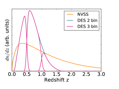
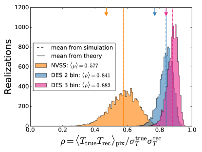
Figure 15: Left panel: Redshift distributions of surveys, chosen to match the LSS surveys studied in Ref. Manzotti and Dodelson (2014). Right panel: Histogram of $\displaystyle\rho$ found for 10,000 simulations of surveys with redshift distributions shown in the left panel. Values of $\displaystyle\bar{\rho}$ from Ref. Manzotti and Dodelson (2014) are shown by the arrows along the top of the plot. The observed discrepancies are likely due to different amounts of simulated galaxy shot noise.

Here we perform a crosscheck of our reconstruction procedure against Manzotti and Dodelson (2014) (MD). In their paper, MD perform simulations for an NVSS-like survey and a DES-like survey in two- and three-binned configurations. We attempt to simulate ISW reconstruction for similar surveys.

For the NVSS-like survey, we use the analytic $\displaystyle dn/dz$ distribution given by MD, integrating between $\displaystyle 0.01\leq z\leq 6$ when computing its $\displaystyle C_{\ell}$. The redshift distributions used for these simulations are shown in the left panel of Fig. 15. For the DES-like survey, we adjusted the parameters in our fiducial $\displaystyle dn/dz$ model by eye so that the three-binned case is similar to that shown in MD’s relevant figure. For the three-binned case, we place bin edges at $\displaystyle z\in[0.1,0.5,1.0,1.6]$. Because MD do not describe how the two-binned case is divided, we somewhat arbitrarily place the bin edges at $\displaystyle z\in[0.1,0.5,1.6]$. Like MD, we include multipoles $\displaystyle 3\leq\ell\leq 80$ in our analysis. We leave $\displaystyle\bar{n}$ at our fiducial value of $\displaystyle 10^{9}$ for all of these surveys. This value was selected based on an assumption that shot noise contributions would be negligible, but we note below that this is likely not the case.

The right panel of Fig. 15 shows a histogram of the $\displaystyle\rho$ values for 10,000 map realizations in our study, with the values from MD shown with arrows. We find that our $\displaystyle\bar{\rho}$ values are systematically higher than, but not wildly incompatible with those in MD. It is hard to specifically identify a cause for this without more information, but the discrepancy is most likely due to differences in the amount of Poisson noise we add to our galaxy maps. We note, for example, that we can get our $\displaystyle\langle\rho\rangle$ for the NVSS-like survey to roughly match the MD value if we reduce our simulation’s $\displaystyle\bar{n}$ to $\displaystyle\sim 5\times 10^{5}$. If we set $\displaystyle\bar{n}$ to the value reported for NVSS by MD, $\displaystyle\bar{n}=5\times 10^{4}\,{\rm sr}^{-1}\approx 16\,{\rm deg}^{-2}$, we get a lower value of $\displaystyle\langle\rho\rangle=0.22$.

The shift between the two- and three-bin DES surveys in our simulations is larger than the $\displaystyle\Delta\rho\sim 0.03$ seen in the binning study of Sec. III.2. This supports our hypothesis that $\displaystyle\bar{\rho}$ shifts more easily at lower $\displaystyle\rho$ values. The fact that our observed shift is still only about half the size of that by MD is probably also due to the fact that we are finding larger $\displaystyle\bar{\rho}$ values than they do.

Appendix B $\displaystyle C_{\ell}$ plots for Sec. IV.1

Figure 16 shows how galaxy-galaxy and galaxy-ISW power spectra respond to changes in the parameters discussed in Sec. IV.1. We study the effect of survey depth by shifting the parameter $\displaystyle z_{0}$ in Eq. (9), redshift dependence of bias by changing $\displaystyle b_{2}$ in Eq. (27), and the fraction of galaxies $\displaystyle x$ subject to catastrophic photometric-redshift errors via Eq. (28).

We see that changing $\displaystyle z_{0}$ and $\displaystyle b_{2}$ shifts $\displaystyle C_{\ell}$ by a mostly scale-independent factor. As noted in Sec. IV.1, this is why systematics related to mismodeling depth and bias redshift dependence have only a small effect on ISW reconstruction quality. It is also why fitting for scale-independent bias $\displaystyle\bar{b}$ via

$$C_{\ell}^{\rm gal(obs)}=\bar{b}^{2}\,C_{\ell}^{\rm gal(model)},$$ (34)

as is discussed in Sec. II.4, protects against these systematics.

In contrast, changing the catastrophic photo-$\displaystyle z$ fraction $\displaystyle x$ by more than about 0.01 significantly changes the low-$\displaystyle\ell$ shape of $\displaystyle C_{\ell}$. This explains why mismodeling $\displaystyle x$ has a relatively larger (though still small) impact on ISW reconstruction quality and why constant bias fitting does not mitigate this effect as much.

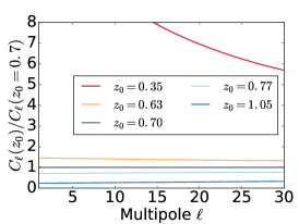
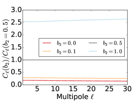
Figure 16: The change in the galaxy angular power spectrum $\displaystyle C_{\ell}\equiv C_{\ell}^{\rm gal-gal}$ in response to (left to right) changes in survey depth, characterized via $\displaystyle z_{0}$ in Eq. (9); the redshift dependence of bias, modeled by varying the $\displaystyle b_{2}$ parameter in $\displaystyle b(z)=1+b_{2}(1+z)^{2}$; and the fraction $\displaystyle x$ of galaxies subject to catastrophic photo-$\displaystyle z$ errors. These plots show the ratio of galaxy autopower relative to that of a reference survey.

Appendix C Calibration error formalism

In Sec. IV.2 we study the impact of photometric calibration errors on ISW signal reconstruction. We model them using a direction-dependent calibration error field $\displaystyle c({\bf\hat{n}})$ via

$$N^{\rm obs}({\bf\hat{n}})=(1+c({\bf\hat{n}}))N({\bf\hat{n}}),$$ (35)

where $\displaystyle{\bf\hat{n}}$ is the direction on the sky, $\displaystyle N^{\rm obs}$ is the observed number of galaxies, and $\displaystyle N$ is the true number of galaxies. Here, we present the calculations necessary to describe how this modifies the galaxy $\displaystyle C_{\ell}$ and which we used above to predict how calibration errors will impact our reconstructions quality statistics. Our notation follows that by Huterer et al. (2013).

We will define fluctuations in the true and observed number density as $\displaystyle\delta$ and $\displaystyle\delta^{\rm obs}$, respectively, and write them in terms of spherical components,

$$\displaystyle\delta({\bf\hat{n}}) \displaystyle=\frac{N({\bf\hat{n}})}{\bar{n}}-1\equiv\sum_{\ell m}g_{\ell m}Y_{\ell m}({\bf\hat{n}})$$ (36)

$$\displaystyle\delta^{\rm obs}({\bf\hat{n}}) \displaystyle=\frac{N^{\rm obs}({\bf\hat{n}})}{\bar{n}^{\rm obs}}-1\equiv\sum_{\ell m}t_{\ell m}Y_{\ell m}.$$ (37)

Additionally, we will define a parameter $\displaystyle\epsilon$ to relate the true and observed average number densities,

$$\bar{n}^{\rm obs}=\bar{n}(1+\epsilon),$$ (38)

and use $\displaystyle c_{\ell m}$ to denote the spherical components of the calibration error field $\displaystyle c({\bf\hat{n}})$. Each galaxy map can have its own calibration error field, and so we will use superscripts (e.g., $\displaystyle g_{\ell m}^{i}$, $\displaystyle c_{\ell m}^{i}$, and $\displaystyle t_{\ell m}^{i}$) to denote components associated with LSS map $\displaystyle i$.

Our goal is to find a relation between the observed galaxy power $\displaystyle T_{\ell}^{ij}$, the true power $\displaystyle C_{\ell}^{ij}$, and the properties of the calibration error field $\displaystyle C_{\ell}^{{\rm cal,}ij}$. To do this, we start by relating the spherical components of the fields. We note that observed number density fluctuations are

$$\delta^{\rm obs}({\bf\hat{n}})=\frac{\delta+c+\delta c-\epsilon}{(1+\epsilon)},$$ (39)

where we suppress the $\displaystyle{\bf\hat{n}}$ arguments to simplify notation. After some algebra, we can write

$$\displaystyle t_{\ell m}^{i}= \displaystyle(1+\epsilon^{i})^{-1}\left[-\sqrt{4\pi}\delta_{\ell 0}\epsilon^{i}+g_{\ell m}^{i}+c_{\ell m}^{i}\right.$$ (40)

$$\displaystyle\left.+\sum_{\ell_{1}\ell_{2}m_{1}m_{2}}\,c^{i}_{\ell_{2}m_{2}}g^{i}_{\ell_{1}m_{1}}\,R^{\ell\ell_{1}\ell_{2}}_{mm_{1}m_{2}}\right].$$ (41)

In this expression, $\displaystyle\delta_{\ell 0}$ is a Kronecker delta, and the multiplicative term

$$R^{\ell\ell_{1}\ell_{2}}_{mm_{1}m_{2}}\equiv\int\,d\Omega Y_{\ell m}^{*}({\bf\hat{n}})\,Y_{\ell_{2}m_{2}}({\bf\hat{n}})\,Y_{\ell_{1}m_{1}}({\bf\hat{n}})$$ (42)

is related to Wigner-3j symbols.

We define the cross-power between two observed maps via

$$T_{\ell}^{ij}\equiv\sum_{m}\frac{\langle t_{\ell m}^{i}t_{\ell m}^{j*}\rangle}{2\ell+1}$$ (43)

and that of the calibration error fields as

$$C_{\ell}^{{\rm cal,}ij}\equiv\sum_{m}\frac{c_{\ell m}^{i}c_{\ell m}^{j*}}{2\ell+1}.$$ (44)

Note that these definitions do not preclude the possibility that the $\displaystyle c_{\ell m}$ could introduce correlations between different ($\displaystyle\ell,m$) modes. The fact that we only show correlations between modes with matching $\displaystyle\ell$ and $\displaystyle m$ reflects the (potentially biased) measurement that would be made even if one assumes that they do not.

The expression for $\displaystyle T_{\ell}^{ij}$ in terms of $\displaystyle g_{\ell m}$, $\displaystyle c_{\ell m}$ is fairly involved, though it can be simplified to some extent using Wigner-3j symbol identities. For the purposes of this paper, we approximate it by only including additive components—that is, neglecting all terms containing $\displaystyle R^{\ell\ell_{1}\ell_{2}}_{mm_{1}m_{2}}$. Doing this, and using the fact that

$$\langle\epsilon^{i}\rangle=\frac{c_{00}^{i}}{\sqrt{4\pi}}=\sqrt{\frac{C^{{\rm cal,}i}_{\ell=0}}{4\pi}},$$ (45)

we write

$$T_{\ell}^{ij}=\frac{C_{\ell}^{gij}+C_{\ell}^{cij}-\delta_{\ell 0}c^{i}_{00}c^{j}_{00}}{(1+c_{00}^{i}/\sqrt{4\pi})(1+c_{00}^{j}/\sqrt{4\pi})}.$$ (46)

This is the expression given in Eq. (30) and is what is used to compute expectations values of ISW reconstruction quality statistics in Sec. IV.2.

Appendix D Large-noise limit of $\displaystyle s$ statistic

In Sec. IV.2.2, and particularly in Fig. 12, we saw that as the amplitude of calibration error fluctuations gets large the ratio between the rms of reconstructed map residuals and the rms of the true ISW map, $\displaystyle s$, approaches a constant value. Here we outline why this occurs.

Recall from Eq. (22) that our theoretical estimator $\displaystyle\langle s\rangle$ is written

$$\langle s\rangle=\frac{\sqrt{\langle\sigma_{\rm rec}\rangle^{2}+\langle\sigma_{\rm ISW}\rangle^{2}-2\,\sum_{\ell i}\,(2\ell+1)\,R_{\ell}^{i}\tilde{C}_{\ell}^{{\rm ISW}-i}}}{\langle\sigma_{\rm ISW}\rangle},$$ (47)

where

$$\displaystyle\langle\sigma_{\rm ISW}\rangle \displaystyle=\sqrt{\sum_{\ell}\,(2\ell+1)\,\tilde{C}_{\ell}^{\rm ISW}}\text{, and}$$ (48)

$$\displaystyle\langle\sigma_{\rm rec}\rangle \displaystyle=\sqrt{\sum_{\ell ij}\,(2\ell+1)\,R_{\ell}^{i}R_{\ell}^{j}\tilde{C}_{\ell}^{ij}}.$$

In the case with a single LSS map, which we focus on here for simplicity, the reconstruction filter is

$$R_{\ell}^{i}=\frac{C_{\ell}^{\rm gal-ISW}}{C_{\ell}^{\rm gal}}.$$ (49)

For clarity, and in contrast with the notation in the main text, here we use tildes (as in $\displaystyle\tilde{C}_{\ell}$) to denote the $\displaystyle C_{\ell}^{\rm true}$ which are associated with observed or simulated maps. The $\displaystyle C_{\ell}$ with no tilde will be the $\displaystyle C_{\ell}^{\rm model}$ used to construct the ISW estimator.

Let us examine how the various terms scale as we increase the amplitude of calibration errors. As the level of calibration errors—or any form of noise—gets large,

$$\tilde{C}_{\rm\ell}^{\rm gal}\stackrel{{\scriptstyle\mathclap{\mbox{\scriptsize large A}}}}{{\hskip 12.80365pt\longrightarrow\hskip 12.80365pt}}C_{\ell}^{\rm noise}\propto A$$ (50)

where $\displaystyle C_{\ell}^{\rm noise}$ is the noise power spectrum and $\displaystyle A$ is a measure of its amplitude. The observed ISW power $\displaystyle\tilde{C}_{\ell}^{\rm ISW}$ and ISW-galaxy cross-power $\displaystyle\tilde{C}_{\ell}^{\rm gal-ISW}$ will not depend on $\displaystyle A$.

For the calibration error studies in Sec. IV.2, we focused on the case of residual calibration errors, which are not accounted for in the ISW estimator. In this scenario, any excess in observed power will be interpreted as a bias and fit for via

$$\bar{b}^{2}C_{\ell}^{\rm gal}=\tilde{C}_{\ell}^{\rm gal},$$ (51)

according to the procedure described in Sec. II.4. Because $\displaystyle C_{\ell}^{\rm gal}$ is independent of $\displaystyle A$, the resulting best fit value will be $\displaystyle\bar{b}^{\rm fit}\propto\sqrt{A}$. The model $\displaystyle C_{\ell}(\bar{b}^{\rm fit})$ scales accordingly,

$$\displaystyle C_{\ell}^{\rm gal}(\bar{b}^{\rm fit}) \displaystyle\propto A,$$ (52)

$$\displaystyle C_{\ell}^{\rm gal-ISW}(\bar{b}^{\rm fit}) \displaystyle\propto\sqrt{A},$$ (53)

$$\displaystyle R_{\ell} \displaystyle\propto\frac{1}{\sqrt{A}}.$$ (54)

Examining the terms in Eq. (47), we see that $\displaystyle\langle\sigma_{\rm rec}\rangle$ and $\displaystyle\langle\sigma_{\rm ISW}\rangle$ will approach constants as $\displaystyle A$ grows, while the cross-term will go to zero like $\displaystyle A^{-1/2}$. Thus, in the case of unmodeled noise contributions to the galaxy maps, in the limit of large noise,

$$\langle s\rangle\stackrel{{\scriptstyle\mathclap{\mbox{\scriptsize large A}}}}{{\hskip 12.80365pt\longrightarrow\hskip 12.80365pt}}\frac{\sqrt{\langle\sigma_{\rm rec}\rangle^{2}+\langle\sigma_{\rm ISW}\rangle^{2}}}{\langle\sigma_{\rm ISW}\rangle}.$$ (55)

This is a constant greater than 1, in agreement with our results in the right panel of Fig. 12.

In contrast, if the $\displaystyle C_{\ell}$ used in the ISW estimator correctly model the level of galaxy noise—as occurs in the shot noise tests in Sec. III.4—the best fit bias parameter $\displaystyle\bar{b}^{\rm fit}$ will remain close to 1. In that case, the fact that noise is properly accounted for means that

$$C_{\ell}^{\rm gal}=\tilde{C}_{\rm ell}^{\rm gal}\propto A$$ (56)

while all other $\displaystyle C_{\ell}$ and $\displaystyle\tilde{C}_{\ell}$ are independent of $\displaystyle A$. In this case, as the noise power dominates over that of galaxies, the estimator operator goes to zero according to

$$R_{\ell}\propto\frac{1}{A}.$$ (57)

This means that for large levels of properly modeled noise, the reconstructed map amplitude goes to zero. This causes $\displaystyle\langle\sigma_{\rm rec}\rangle$ and the cross-term in $\displaystyle\langle s\rangle$ to go to zero and so the reconstruction residuals are just a measure of the true ISW map:

$$\langle s\rangle\stackrel{{\scriptstyle\mathclap{\mbox{\scriptsize large A}}}}{{\hskip 12.80365pt\longrightarrow\hskip 12.80365pt}}\frac{\sqrt{\langle\sigma_{\rm ISW}\rangle^{2}}}{\langle\sigma_{\rm ISW}\rangle}=1.$$ (58)

References

- Hu and Sugiyama (1994) W. Hu and N. Sugiyama, Phys. Rev. D50, 627 (1994), arXiv:astro-ph/9310046 [astro-ph] .
- Sachs and Wolfe (1967) R. Sachs and A. Wolfe, Astrophys.J. 147, 73 (1967).
- Bean and Dore (2004) R. Bean and O. Dore, Phys. Rev. D69, 083503 (2004), arXiv:astro-ph/0307100 [astro-ph] .
- Weller and Lewis (2003) J. Weller and A. M. Lewis, Mon. Not. Roy. Astron. Soc. 346, 987 (2003), arXiv:astro-ph/0307104 [astro-ph] .
- Song et al. (2007) Y.-S. Song, I. Sawicki, and W. Hu, Phys. Rev. D75, 064003 (2007), arXiv:astro-ph/0606286 [astro-ph] .
- Crittenden and Turok (1996) R. G. Crittenden and N. Turok, Phys.Rev.Lett. 76, 575 (1996), arXiv:astro-ph/9510072 [astro-ph] .
- Boughn and Crittenden (2004) S. Boughn and R. Crittenden, Nature 427, 45 (2004), arXiv:astro-ph/0305001 [astro-ph] .
- Fosalba et al. (2003) P. Fosalba, E. Gaztanaga, and F. Castander, Astrophys. J. 597, L89 (2003), arXiv:astro-ph/0307249 [astro-ph] .
- Nolta et al. (2004) M. R. Nolta et al. (WMAP), Astrophys. J. 608, 10 (2004), arXiv:astro-ph/0305097 [astro-ph] .
- Corasaniti et al. (2005) P.-S. Corasaniti, T. Giannantonio, and A. Melchiorri, Phys. Rev. D71, 123521 (2005), arXiv:astro-ph/0504115 [astro-ph] .
- Padmanabhan et al. (2005) N. Padmanabhan, C. M. Hirata, U. Seljak, D. Schlegel, J. Brinkmann, and D. P. Schneider, Phys. Rev. D72, 043525 (2005), arXiv:astro-ph/0410360 [astro-ph] .
- Vielva et al. (2006) P. Vielva, E. Martinez-Gonzalez, and M. Tucci, Mon. Not. Roy. Astron. Soc. 365, 891 (2006), arXiv:astro-ph/0408252 [astro-ph] .
- McEwen et al. (2007) J. D. McEwen, P. Vielva, M. P. Hobson, E. Martinez-Gonzalez, and A. N. Lasenby, Mon. Not. Roy. Astron. Soc. 376, 1211 (2007), arXiv:astro-ph/0602398 [astro-ph] .
- Giannantonio et al. (2006) T. Giannantonio, R. G. Crittenden, R. C. Nichol, R. Scranton, G. T. Richards, A. D. Myers, R. J. Brunner, A. G. Gray, A. J. Connolly, and D. P. Schneider, Phys. Rev. D74, 063520 (2006), arXiv:astro-ph/0607572 [astro-ph] .
- Cabre et al. (2007) A. Cabre, P. Fosalba, E. Gaztanaga, and M. Manera, Mon.Not.Roy.Astron.Soc. 381, 1347 (2007), arXiv:astro-ph/0701393 [astro-ph] .
- Rassat et al. (2007) A. Rassat, K. Land, O. Lahav, and F. B. Abdalla, Mon. Not. Roy. Astron. Soc. 377, 1085 (2007), arXiv:astro-ph/0610911 [astro-ph] .
- Giannantonio et al. (2008) T. Giannantonio, R. Scranton, R. G. Crittenden, R. C. Nichol, S. P. Boughn, et al., Phys.Rev. D77, 123520 (2008), arXiv:0801.4380 [astro-ph] .
- Ho et al. (2008) S. Ho, C. Hirata, N. Padmanabhan, U. Seljak, and N. Bahcall, Phys. Rev. D78, 043519 (2008), arXiv:0801.0642 [astro-ph] .
- Xia et al. (2009) J.-Q. Xia, M. Viel, C. Baccigalupi, and S. Matarrese, JCAP 0909, 003 (2009), arXiv:0907.4753 [astro-ph.CO] .
- Giannantonio et al. (2012) T. Giannantonio, R. Crittenden, R. Nichol, and A. J. Ross, Mon.Not.Roy.Astron.Soc. 426, 2581 (2012), arXiv:1209.2125 [astro-ph.CO] .
- Ade et al. (2014) P. Ade et al. (Planck Collaboration), Astron.Astrophys. 571, A19 (2014), arXiv:1303.5079 [astro-ph.CO] .
- Ade et al. (2015a) P. Ade et al. (Planck Collaboration), (2015a), arXiv:1502.01595 [astro-ph.CO] .
- Dupe et al. (2011) F.-X. Dupe, A. Rassat, J.-L. Starck, and M. Fadili, Astron.Astrophys. 534, 51 (2011), arXiv:1010.2192 [astro-ph.CO] .
- Hu and Scranton (2004) W. Hu and R. Scranton, Phys. Rev. D70, 123002 (2004), arXiv:astro-ph/0408456 .
- Schwarz et al. (2015) D. J. Schwarz, C. J. Copi, D. Huterer, and G. D. Starkman (2015) arXiv:1510.07929 [astro-ph.CO] .
- Francis and Peacock (2010) C. Francis and J. Peacock, Mon.Not.Roy.Astron.Soc. 406, 14 (2010), arXiv:0909.2495 [astro-ph.CO] .
- Rassat et al. (2013) A. Rassat, J. L. Starck, and F. X. Dupe, Astron.Astrophys. 557, A32 (2013), arXiv:1303.4727 [astro-ph.CO] .
- Ade et al. (2015b) P. A. R. Ade et al. (Planck), (2015b), arXiv:1502.01592 [astro-ph.CO] .
- Kim et al. (2013) J. Kim, A. Rotti, and E. Komatsu, JCAP 1304, 021 (2013), arXiv:1302.5799 [astro-ph.CO] .
- Manzotti and Dodelson (2014) A. Manzotti and S. Dodelson, Phys.Rev. D90, 123009 (2014), arXiv:1407.5623 [astro-ph.CO] .
- Bonavera et al. (2016) L. Bonavera, R. B. Barreiro, A. Marcos-Caballero, and P. Vielva, Mon. Not. Roy. Astron. Soc. 459, 657 (2016), arXiv:1602.05893 [astro-ph.CO] .
- Afshordi (2004) N. Afshordi, Phys. Rev. D70, 083536 (2004), arXiv:astro-ph/0401166 [astro-ph] .
- LoVerde and Afshordi (2008) M. LoVerde and N. Afshordi, Phys. Rev. D78, 123506 (2008), arXiv:0809.5112 [astro-ph] .
- Lesgourgues (2011) J. Lesgourgues, (2011), arXiv:1104.2932 [astro-ph.IM] .
- Gorski et al. (2005) K. M. Gorski, E. Hivon, A. J. Banday, B. D. Wandelt, F. K. Hansen, M. Reinecke, and M. Bartelman, Astrophys. J. 622, 759 (2005), arXiv:astro-ph/0409513 [astro-ph] .
- Laureijs et al. (2011) R. Laureijs et al. (EUCLID), (2011), arXiv:1110.3193 [astro-ph.CO] .
- Douspis et al. (2008) M. Douspis, P. G. Castro, C. Caprini, and N. Aghanim, Astron. Astrophys. 485, 395 (2008), arXiv:0802.0983 [astro-ph] .
- Martinet et al. (2015) N. Martinet, J. G. Bartlett, A. Kiessling, and B. Sartoris, Astron. Astrophys. 581, A101 (2015), arXiv:1506.02192 [astro-ph.CO] .
- Becker et al. (2015) M. R. Becker et al. (DES), (2015), arXiv:1507.05598 [astro-ph.CO] .
- Cimatti et al. (2009) A. Cimatti, R. Laureijs, B. Leibundgut, S. Lilly, R. Nichol, A. Refregier, P. Rosati, M. Steinmetz, N. Thatte, and E. Valentijn, (2009), arXiv:0912.0914 [astro-ph.CO] .
- Hu (1999) W. Hu, Astrophys. J. 522, L21 (1999), arXiv:astro-ph/9904153 [astro-ph] .
- Ma et al. (2005) Z.-M. Ma, W. Hu, and D. Huterer, Astrophys. J. 636, 21 (2005), arXiv:astro-ph/0506614 [astro-ph] .
- Bernstein and Huterer (2010) G. Bernstein and D. Huterer, Mon. Not. Roy. Astron. Soc. 401, 1399 (2010), arXiv:0902.2782 [astro-ph.CO] .
- Hearin et al. (2010) A. P. Hearin, A. R. Zentner, Z. Ma, and D. Huterer, Astrophys. J. 720, 1351 (2010), arXiv:1002.3383 [astro-ph.CO] .
- Hildebrandt et al. (2012) H. Hildebrandt et al., Mon. Not. Roy. Astron. Soc. 421, 2355 (2012), arXiv:1111.4434 [astro-ph.CO] .
- Pullen and Hirata (2013) A. R. Pullen and C. M. Hirata, Publications of the Astronomical Society of the Pacific, Volume 125, Issue 928, pp. 705-718 (2013), 10.1086/671189, arXiv:1212.4500 [astro-ph.CO] .
- Ho et al. (2012) S. Ho, A. Cuesta, H.-J. Seo, R. de Putter, A. J. Ross, et al., Astrophys.J. 761, 14 (2012), arXiv:1201.2137 [astro-ph.CO] .
- Ho et al. (2013) S. Ho, N. Agarwal, A. D. Myers, R. Lyons, A. Disbrow, et al., 1311.2597 (2013), arXiv:1311.2597 [astro-ph.CO] .
- Agarwal et al. (2014a) N. Agarwal, S. Ho, and S. Shandera, JCAP 1402, 038 (2014a), arXiv:1311.2606 [astro-ph.CO] .
- Giannantonio et al. (2014) T. Giannantonio, A. J. Ross, W. J. Percival, R. Crittenden, D. Bacher, et al., Phys.Rev. D89, 023511 (2014), arXiv:1303.1349 [astro-ph.CO] .
- Agarwal et al. (2014b) N. Agarwal, S. Ho, A. D. Myers, H.-J. Seo, A. J. Ross, et al., JCAP 1404, 007 (2014b), arXiv:1309.2954 [astro-ph.CO] .
- Huterer et al. (2013) D. Huterer, C. E. Cunha, and W. Fang, Mon.Not.Roy.Astron.Soc. 432, 2945 (2013), arXiv:1211.1015 [astro-ph.CO] .
- Leistedt et al. (2013) B. Leistedt, H. V. Peiris, D. J. Mortlock, A. Benoit-Lévy, and A. Pontzen, Mon.Not.Roy.Astron.Soc. 435, 1857 (2013), arXiv:1306.0005 [astro-ph.CO] .
- Leistedt and Peiris (2014) B. Leistedt and H. V. Peiris, Mon.Not.Roy.Astron.Soc. 444, 2 (2014), arXiv:1404.6530 [astro-ph.CO] .
- Shafer and Huterer (2015) D. L. Shafer and D. Huterer, Mon. Not. Roy. Astron. Soc. 447, 2961 (2015), arXiv:1410.0035 [astro-ph.CO] .
- Jouvel et al. (2009) S. Jouvel et al., Astron. Astrophys. 504, 359 (2009), arXiv:0902.0625 [astro-ph.CO] .
- Rykoff et al. (2015) E. S. Rykoff, E. Rozo, and R. Keisler, ArXiv e-prints (2015), arXiv:1509.00870 [astro-ph.IM] .
- Padmanabhan et al. (2008) N. Padmanabhan et al., Astrophys. J. 674, 1217 (2008), arXiv:astro-ph/0703454 [ASTRO-PH] .
- Copi et al. (2015) C. J. Copi, D. Huterer, D. J. Schwarz, and G. D. Starkman, Mon. Not. Roy. Astron. Soc. 449, 3458 (2015), arXiv:1311.4562 [astro-ph.CO] .
- de Oliveira-Costa et al. (2004) A. de Oliveira-Costa, M. Tegmark, M. Zaldarriaga, and A. Hamilton, Phys. Rev. D69, 063516 (2004), arXiv:astro-ph/0307282 [astro-ph] .
- Copi et al. (2006) C. J. Copi, D. Huterer, D. J. Schwarz, and G. D. Starkman, Mon. Not. Roy. Astron. Soc. 367, 79 (2006), arXiv:astro-ph/0508047 [astro-ph] .