Exact results for ABJ Wilson loops and open-closed duality

Abstract

We find new exact relations between the partition function and vacuum expectation values (VEVs) of 1/2 BPS Wilson loops in ABJ theory, which allow us to predict the large $N$ expansions of the 1/2 BPS Wilson loops from known results of the partition function. These relations are interpreted as an open-closed duality where the closed string background is shifted by the insertion of Wilson loops due to a back-reaction. Using the connection between ABJ theory and the topological string on local $\mathbb{P}^{1}\times\mathbb{P}^{1}$, we explicitly write down non-trivial relations between open and closed string amplitudes.

1 Introduction

This work addresses exact computations of Wilson loops in ABJ(M) theory ABJM ; ABJ . Our analysis heavily relies on the supersymmetric localization Pestun . The ABJ theory is a 3d $\mathcal{N}=6$ superconformal Chern-Simons-matter theory with quiver gauge group $U(N_{1})_{k}\times U(N_{2})_{-k}$, which describes a low energy effective theory on multiple M2-branes. When the ranks of the two gauge groups are equal, the theory is especially called the ABJM theory. As shown in KWY1 ; Jafferis ; HHL1 , the partition function of ABJ theory (and more generally for a wider class of Chern-Simons-matter theories) on a three-sphere reduces to a matrix integral by the localization. A basic problem is then to understand the large $N$ behavior of the obtained matrix model.

To extract the information at large $N$ from the ABJ matrix model, one can use two remarkable facts. One is a connection with the topological string on a particular Calabi-Yau three-fold, known as local $\mathbb{P}^{1}\times\mathbb{P}^{1}$. This connection is a consequence of a chain of dualities: The ABJ matrix model is related to a matrix model on a lens space $L(2,1)$ by analytic continuation MP-top . It is known that this lens space matrix model is dual to the topological string on local $\mathbb{P}^{1}\times\mathbb{P}^{1}$ at large $N$ AKMV . As a result, the large $N$ expansion in the ABJ matrix model is captured by the topological string on local $\mathbb{P}^{1}\times\mathbb{P}^{1}$. The all-genus free energy in the ’t Hooft limit was indeed computed in DMP1 by using the topological string technique. The planar free energy shows the $N^{3/2}$ behavior, which correctly reproduces the expected number of degrees of freedom of $N$ M2-branes. The same behavior was also confirmed by the direct saddle-point analysis in the M-theory limit HKPT .

Another key fact is an unexpected relation to a non-interacting quantum Fermi-gas system. It was shown in MP that the ABJM partition function is regarded as the partition function of an ideal quantum Fermi-gas with an unconventional Hamiltonian. This Fermi-gas picture allows us to analyze the system by the technique of statistical mechanics. The important point is that the role of the Planck constant in this quantum system is played by the Chern-Simons level, and the semi-classical limit corresponds to the strong coupling limit in ABJM theory. Therefore we can get the strong coupling results from the semi-classical analysis in the Fermi-gas system. Putting the various pieces of information together (see HMO-review for a review and references therein), it was finally shown in HMMO that the complete large $N$ expansion, including both worldsheet instanton and membrane instanton corrections, of the partition function are determined by the (refined) topological string on local $\mathbb{P}^{1}\times\mathbb{P}^{1}$ in a highly non-trivial way. Quite interestingly, there is a pole cancellation mechanism between the worldsheet instanton corrections and the membrane instanton corrections HMO2 , which guarantees the theory to be well-defined for any value of $k$. The Fermi-gas approach was also extended to the ABJ matrix model MaMo ; HoOk (see also AHS ; Honda1 ), and it was revealed that the large $N$ expansion is again determined by the topological string on local $\mathbb{P}^{1}\times\mathbb{P}^{1}$.

In this paper, we study circular BPS Wilson loops in ABJ theory on $S^{3}$. There are two kinds of BPS Wilson loops in ABJ theory. One preserves 1/6 of supersymmetries DPY ; CW ; RSY , while the other a half of them DT . We here focus on the latter since it has a much simpler structure than the former. The vacuum expectation values (VEVs) of BPS Wilson loops can be exactly computed by the localization. The Fermi-gas approach for the Wilson loops in ABJM theory was first proposed in KMSS and a similar formalism was further developed in HHMO especially for the 1/2 BPS Wilson loops. It was shown in MP-top that the large $N$ expansions of the 1/2 BPS Wilson loops are explained by the open topological string on local $\mathbb{P}^{1}\times\mathbb{P}^{1}$. The Seiberg-like duality of the ABJ Wilson loops was discussed in HNS .

It is known that the ABJ partition function has several good properties. For some particular values of $k$, the generating function of the partition function can be written in closed form CGM ; GHM2 . This fact enables us to predict the exact values of the partition function without performing the matrix integral. It was also found in GHM2 that the generating function of the ABJ partition function satisfies beautiful functional relations. Therefore it is natural to ask whether the Wilson loops in ABJ theory also have some nice properties or not. As we will show in this paper, the answer is yes: We find remarkable exact relations among the 1/2 BPS Wilson loops!

Based on the previous analysis in MaMo ; HoOk ; HHMO , we here find new exact relations between the partition function and the VEVs of the 1/2 BPS Wilson loops. In the simplest case, the VEV of the 1/2 BPS Wilson loop with the fundamental representation in $U(N)_{k}\times U(N)_{-k}$ ABJM theory is exactly related to the partition function of $U(N-1)_{k}\times U(N+1)_{-k}$ ABJ theory. Namely, the normalized VEV of the fundamental ABJM Wilson loop is given by

$$\langle W_{\vbox{\offinterlineskip\kern 1.0pt\hbox{\kern 1.0pt\vbox{\hbox{\noindent\vbox{\hbox{\vbox to0.0pt{\hrule height=0.4pt,width=3.90555pt\vss}}\hbox{\vbox{\hbox to0.0pt{\vrule width=0.4pt,height=3.90555pt\hss}}\kern 3.90555pt\vbox{\hbox to0.0pt{\vrule width=0.4pt,height=3.90555pt\hss}}}\hbox{\vbox{\hbox{\vbox to0.0pt{\hrule height=0.4pt,width=4.30554pt\vss}}}\kern-0.4pt}}}\hbox{} }\kern 1.0pt\kern 0.4pt}\kern 1.0pt\kern 0.4pt}}^{(1/2)}\rangle_{N,k}^{\text{ABJM}}=\frac{1}{2\sin\frac{2\pi}{k}}\biggl{|}\frac{Z^{\text{ABJ}}(N-1,N+1,k)}{Z^{\text{ABJM}}(N,k)}\biggr{|}.$$ (1)

We conjecture that this relation holds for any $N$ and $k(>2)$. In the large $N$ limit, the all-order perturbative $1/N$ expansion of the free energy can be resummed, and it results in the Airy functional form FHM . As shown in KMSS , the VEVs of the 1/2 BPS Wilson loops are also resummed as the Airy function, and the final result in KMSS is consistent with our exact relation (1). We stress that our relation (1), however, contains all the non-perturbative corrections, and it is true even for finite $N$. As we will see in section 3, the relation (1) is only a tip of the iceberg. We find many similar relations for higher representations in the ABJ Wilson loops, as shown in Fig. 1. We also find a determinant formula that computes the VEVs of the 1/2 BPS Wilson loops with general representations only from “hook” representations. This is a natural generalization of the result in HHMO to the ABJ Wilson loops.

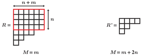
Figure 1: The VEV of the 1/2 BPS Wilson loop with the left Young diagram $R$ in $M=m$ ABJ theory is related to the one with the right diagram $R^{\prime}$ in $M=m+2n$ ABJ theory. In other words, the effect of the red rectangular part in $R$ results in adding the $2n$ fractional M2-branes after the back-reaction. The relation (1) corresponds to the simplest case that $n=1$, $m=0$ and $R^{\prime}$ is the trivial representation.

The relation (1) has the following interpretation: From the viewpoint of type IIA string theory on $AdS_{4}\times\mathbb{CP}^{3}$, which is holographically dual to ABJ theory on $S^{3}$, the left hand side of (1) is related to the fundamental open string. On the other hand, the right hand side of (1) is purely explained by a change of the closed string background, where the value of the NSNS B-field flux through a two-cycle $\mathbb{CP}^{1}\subset\mathbb{CP}^{3}$

$$\int_{\mathbb{CP}^{1}}B_{\text{NS}}=\frac{1}{2}-\frac{M}{k},\qquad M=N_{2}-N_{1}.$$ (2)

is shifted from $M=0$ to $M=2$ by inserting the fundamental Wilson loop. In this sense, we can regard (1) as a kind of open-closed dualities. In the brane setup, $M$ counts the number of fractional M2-branes ABJ . Our relation (1) implies that the effect of the brane that describes the fundamental Wilson loop in ABJM theory results in two fractional branes in ABJ theory due to the back-reaction. Roughly speaking, if the dimension of the representation in the Wilson loop grows, then the number of the fractional branes also increases, as in Fig. 1.

The open-closed duality here is also understood from the topological string perspective. As mentioned above, the left hand side of (1) corresponds to the open topological string MP-top ; GKM ; HHMO , while the right hand side is captured by the closed topological string HMMO ; HoOk . Thus, we find that the open topological string amplitude on local $\mathbb{P}^{1}\times\mathbb{P}^{1}$ is related to the closed string amplitude on the same Calabi-Yau. As explained in ADKMV , the effect of the open string generally leads to a shift of certain moduli of the closed string, i.e., the open string amplitude is schematically written as

$$Z_{\text{open}}(Q)=\frac{Z_{\text{closed}}(Q^{\prime})}{Z_{\text{closed}}(Q)},$$ (3)

where $Q$ and $Q^{\prime}$ are moduli of the (same) Calabi-Yau manifold. Our relation is a concrete realization of this open-closed duality at the quantitative level. In section 5, we will explicitly show that (1) leads to the non-trivial relation (144) between the open and closed string amplitudes. Also, the relation in Fig. 1 is easily translated into the topological string language (153).

The organization of this paper is as follows. In the next section, we briefly review the 1/2 BPS Wilson loops in ABJ theory. We mainly use the Fermi-gas formalism proposed in MaMo . In section 3, we demonstrate that the ABJ Wilson loops for different $M$’s are interrelated. In some cases, the relations reduce to the ones between the partition function and the Wilson loops, and we can interpret them as an open-closed duality. In section 4, we show additional results for $k\in 4\mathbb{N}$. In section 5, we consider a consequence of the relations found in section 3. We explicitly show that the open topological string partition function is related to the closed one. We conclude in section 6 and comment on some future directions.

2 A review of ABJ Wilson loops

Let us start with a review of the Wilson loops in ABJ theory.

2.1 ABJ Wilson loops

In ABJ theory, two kinds of circular BPS Wilson loops are widely studied in the literature. One preserves only 1/6 of supersymmetries, while the other a half of supersymmetries. The 1/6 BPS Wilson loops is explicitly given by

$$W_{R}^{(1/6)}=\operatorname{Tr}_{R}\operatorname{Pexp}\left[\int\!{\rm d}s\left({\rm i}A_{\mu}\dot{x}^{\mu}+\frac{2\pi}{k}|\dot{x}|M^{I}_{J}C_{I}\bar{C}^{J}\right)\right],$$ (4)

where $x^{\mu}(s)$ parametrizes a great circle of $S^{3}$, and $C_{I}$ ($I=1,2,3,4$) are scalar fields in the four bi-fundamental chiral multiplets. The matrix $M^{I}_{J}$ is chosen in order to preserve the supersymmetry. The construction of the 1/2 BPS Wilson loops is more complicated. See DT for detail.

The localization method allows us to reduce the path integral to a finite-dimensional matrix integral. The partition function of ABJ theory on $S^{3}$ is exactly given by

$$Z^{\text{ABJ}}(N_{1},N_{2},k)=\frac{{\rm i}^{-\frac{1}{2}(N_{1}^{2}-N_{2}^{2})}}{N_{1}!N_{2}!}\int\!\prod_{i=1}^{N_{1}}\frac{{\rm d}\mu_{i}}{2\pi}\prod_{j=1}^{N_{2}}\frac{{\rm d}\nu_{j}}{2\pi}\,{\rm e}^{-\frac{{\rm i}k}{4\pi}(\sum_{i}\mu_{i}^{2}-\sum_{j}\nu_{j}^{2})}$$ (5)

$$\times\frac{\prod_{i<j}(2\sinh\frac{\mu_{i}-\mu_{j}}{2})^{2}(2\sinh\frac{\nu_{i}-\nu_{j}}{2})^{2}}{\prod_{i,j}(2\cosh\frac{\mu_{i}-\nu_{j}}{2})^{2}}.$$

In the analysis below, we always assume that $k>0$ and $N_{1}\leq N_{2}$ without loss of generality. Sometimes it is convenient to parametrize $N_{1}$ and $N_{2}$ by

$$N_{1}=N,\qquad N_{2}=N+M,\qquad M\geq 0.$$ (6)

Physically, $M$ corresponds to the number of fractional M2-branes ABJ . It was shown in KWY1 that the VEVs of the 1/6 BPS Wilson loops are given by the insertion of an operator in the above matrix model

$$\langle W_{R}^{(1/6)}\rangle_{N_{1},N_{2},k}=\langle s_{R}({\rm e}^{\mu_{1}},\dots,{\rm e}^{\mu_{N_{1}}})\rangle,$$ (7)

where $s_{R}({\rm e}^{\mu_{1}},\dots,{\rm e}^{\mu_{N_{1}}})$ is the Schur polynomial with representation $R$ in $U(N_{1})$. The expectation values on the right hand side means the unnormalized VEV for the ABJ matrix model (5). Of course one can consider an insertion in the other gauge group $U(N_{2})$.

The VEVs of the 1/2 BPS Wilson loops are also given by the insertion of the character of the supergroup $U(N_{1}|N_{2})$ DT . Since the character of the supergroup $U(N_{1}|N_{2})$ is given by the supersymmetric Schur polynomial, we have

$$\langle W_{R}^{(1/2)}\rangle_{N_{1},N_{2},k}=\langle s_{R}({\rm e}^{\mu_{1}},\dots,{\rm e}^{\mu_{N_{1}}}/{\rm e}^{\nu_{1}},\dots,{\rm e}^{\nu_{N_{2}}})\rangle,$$ (8)

where $s_{R}({\rm e}^{\mu_{1}},\dots,{\rm e}^{\mu_{N_{1}}}/{\rm e}^{\nu_{1}},\dots,{\rm e}^{\nu_{N_{2}}})$ is the super Schur polynomial associated with the representation $R$ in supergroup $U(N_{1}|N_{2})$, which is related to the standard Schur polynomial by

$$s_{\lambda}(x/y)=\sum_{\mu,\nu}N_{\mu\nu}^{\lambda}s_{\mu}(x)s_{\nu^{T}}(y).$$ (9)

Here $N_{\mu\nu}^{\lambda}$ is the Littlewood-Richardson coefficient, and $\lambda^{T}$ means the conjugate (or transposed) partition of $\lambda$. Note that the super Schur polynomial satisfies a conjugation formula

$$s_{\lambda}(x/y)=s_{\lambda^{T}}(y/x).$$ (10)

Before reviewing the exact computation of the VEVs of the 1/2 BPS Wilson loops, let us explain a convention of representations. In this paper, we often use the so-called Frobenius notation of representations. The standard Frobenius notation for the partition $\lambda=[\lambda_{1}\lambda_{2}\lambda_{3}\dots]$ is denoted by $(a_{1}\dots a_{r}|l_{1}\dots l_{r})$, where $a_{q}$ and $l_{p}$ are given by

$$a_{q}=\lambda_{q}-q,\qquad l_{p}=\lambda^{T}_{p}-p.$$ (11)

Here $\lambda^{T}=[\lambda^{T}_{1}\lambda^{T}_{2}\lambda^{T}_{3}\dots]$ is the conjugate partition of $\lambda$. The maximal value $r$ is defined by

$$r=\max\{s|\lambda_{s}-s\geq 0\}.$$ (12)

In MaMo , a modification of the Frobenius notation was also introduced. For a given non-negative integer $M$, we define $\widehat{a}_{q}$ and $\widehat{l}_{p}$ by

$$\widehat{a}_{q}=\lambda_{q}-q-M,\qquad\widehat{l}_{p}=\lambda^{T}_{p}-p+M.$$ (13)

Then, the modified Frobenius notation of $\lambda$ is denoted by $(\widehat{a}_{1}\dots\widehat{a}_{r_{M}}|\widehat{l}_{1}\dots\widehat{l}_{r_{M}+M})$, where $r_{M}$ is now

$$r_{M}=\max\{s|\lambda_{s}-s-M\geq 0\}.$$ (14)

If $\lambda_{1}\leq M$, we define $r_{M}=0$, and denote the modified Frobenius notation by $(|\widehat{l}_{1}\dots\widehat{l}_{M})$. Of course, for $M=0$, the modified Frobenius notation is identical to the standard Frobenius notation. Let us see an example. For the representation $R=[2,2,1]=\vbox{\offinterlineskip\kern 1.0pt\hbox{\kern 1.0pt\vbox{\hbox{\noindent\vbox{\hbox{\vbox to0.0pt{\hrule height=0.4pt,width=3.90555pt\vss}}\hbox{\vbox{\hbox to0.0pt{\vrule width=0.4pt,height=3.90555pt\hss}}\kern 3.90555pt\vbox{\hbox to0.0pt{\vrule width=0.4pt,height=3.90555pt\hss}}}\hbox{\vbox{\hbox{\vbox to0.0pt{\hrule height=0.4pt,width=4.30554pt\vss}}}\kern-0.4pt}}\vbox{\hbox{\vbox to0.0pt{\hrule height=0.4pt,width=3.90555pt\vss}}\hbox{\vbox{\hbox to0.0pt{\vrule width=0.4pt,height=3.90555pt\hss}}\kern 3.90555pt\vbox{\hbox to0.0pt{\vrule width=0.4pt,height=3.90555pt\hss}}}\hbox{\vbox{\hbox{\vbox to0.0pt{\hrule height=0.4pt,width=4.30554pt\vss}}}\kern-0.4pt}}}\hbox{\noindent\vbox{\hbox{\vbox to0.0pt{\hrule height=0.4pt,width=3.90555pt\vss}}\hbox{\vbox{\hbox to0.0pt{\vrule width=0.4pt,height=3.90555pt\hss}}\kern 3.90555pt\vbox{\hbox to0.0pt{\vrule width=0.4pt,height=3.90555pt\hss}}}\hbox{\vbox{\hbox{\vbox to0.0pt{\hrule height=0.4pt,width=4.30554pt\vss}}}\kern-0.4pt}}\vbox{\hbox{\vbox to0.0pt{\hrule height=0.4pt,width=3.90555pt\vss}}\hbox{\vbox{\hbox to0.0pt{\vrule width=0.4pt,height=3.90555pt\hss}}\kern 3.90555pt\vbox{\hbox to0.0pt{\vrule width=0.4pt,height=3.90555pt\hss}}}\hbox{\vbox{\hbox{\vbox to0.0pt{\hrule height=0.4pt,width=4.30554pt\vss}}}\kern-0.4pt}}}\hbox{\noindent\vbox{\hbox{\vbox to0.0pt{\hrule height=0.4pt,width=3.90555pt\vss}}\hbox{\vbox{\hbox to0.0pt{\vrule width=0.4pt,height=3.90555pt\hss}}\kern 3.90555pt\vbox{\hbox to0.0pt{\vrule width=0.4pt,height=3.90555pt\hss}}}\hbox{\vbox{\hbox{\vbox to0.0pt{\hrule height=0.4pt,width=4.30554pt\vss}}}\kern-0.4pt}}}\hbox{} }\kern 1.0pt\kern 0.4pt}\kern 1.0pt\kern 0.4pt}$, the standard Frobenius notation is $(10|20)$. For $M=1$, the modified Frobenius notation of the same representation is $(0|31)$, and for $M=2,3$, one finds $(|42)$ and $(|530)$, respectively. See Fig. 1 in MaMo for more details.

2.2 Fermi-gas formalism

It is not easy to evaluate the ABJ matrix model (5) directly. Fortunately, there is a powerful method to evaluate it, known as the Fermi-gas formalism MP . This formalism can be generalized to the Wilson loops KMSS ; HHMO ; MaMo . Here we will briefly review that formalism.

2.2.1 Generating function with phase factor

Our main goal is to evaluate the unnormalized VEVs (8) systematically. To do so, we use the nice formalism in MaMo . Let us define a generating function of the VEVs of the $1/2$ BPS Wilson loops with representation $R$ by

$$\mathcal{W}_{R}^{\text{phase}}(\kappa,k,M)=\sum_{N=0}^{\infty}\kappa^{N}\langle W_{R}^{(1/2)}\rangle_{N_{1}=N,N_{2}=N+M,k}\,,$$ (15)

where we call $\kappa$ the fugacity by analogy with the grand canonical ensemble. Below, we use both the fugacity $\kappa$ and the chemical potential $\mu=\log\kappa$ interchangeably. We also introduce the grand canonical partition function by

$$\Xi^{\text{phase}}(\kappa,k,M)=\sum_{N=0}^{\infty}\kappa^{N}Z^{\text{ABJ}}(N,N+M,k).$$ (16)

In general, the partition function $Z^{\text{ABJ}}(N,N+M,k)$ and the VEV $\langle W_{R}^{(1/2)}\rangle_{N,N+M,k}$ are complex-valued, and have a non-trivial phase. Hence we put the superscript “phase” in (15) and (16). As shown in AHS ; HoOk , the ABJ partition function (5) can be written as

$$Z^{\text{ABJ}}(N,N+M,k)={\rm e}^{{\rm i}\theta_{0}(k,M)}{\rm e}^{\frac{\pi{\rm i}}{2}MN}Z^{\text{CS}}(k,M)\widehat{Z}(N,N+M,k),$$ (17)

where ${\rm e}^{{\rm i}\theta_{0}(k,M)}$ is a phase factor,

$$\begin{aligned} {\rm e}^{{\rm i}\theta_{0}(M,k)}=\exp\left[-\frac{\pi{\rm i}M(M^{2}-1)}{6k}+\frac{\pi{\rm i}M(M-2)}{4}\right],\end{aligned}$$ (18)

and $Z^{\text{CS}}(k,M)$ is the partition function of the pure $U(M)$ Chern-Simons (CS) theory

$$Z^{\text{CS}}(k,M)=k^{-M/2}\prod_{s=1}^{M-1}\left(2\sin\frac{\pi s}{k}\right)^{M-s}.$$ (19)

Note that $\widehat{Z}(N,N+M,k)$ always takes a real value and obeys

$$\widehat{Z}(0,M,k)=1.$$ (20)

It is also convenient to introduce generating functions of the absolute value $|Z^{\text{ABJ}}(N,N+M,k)|$ and of the rescaled partition function divided by the pure CS factor,

$$\Xi_{0}(\kappa,k,M) =\sum_{N=0}^{\infty}\kappa^{N}|Z^{\text{ABJ}}(N,N+M,k)|,$$ (21)

$$\Xi(\kappa,k,M) =\frac{\Xi_{0}(\kappa,k,M)}{Z^{\text{CS}}(k,M)}=1+\sum_{N=1}^{\infty}\kappa^{N}\widehat{Z}(N,N+M,k),$$

but for the moment we will consider the grand partition function (16) with phase. For the ABJM case $M=0$, the phase factor and the pure CS partition function are trivial, and all the definitions in (16) and (21) are identical

$$\Xi^{\text{phase}}(\kappa,k,0)=\Xi_{0}(\kappa,k,0)=\Xi(\kappa,k,0).$$ (22)

However, they are different for the general ABJ case with $M\not=0$.

Formalism of Matsumoto-Moriyama.

In MaMo , it was shown that the generating function (15) is given by a determinant of an $(M+r_{M})\times(M+r_{M})$ matrix,

$$\mathcal{W}_{R}^{\text{phase}}(\kappa,k,M)=\Xi_{0}(\kappa,k,0)\det\Bigl{(}(H_{\widehat{l}_{p},M-q})_{1\leq q\leq M}\Bigl{|}(\widetilde{H}_{\widehat{l}_{p},\widehat{a}_{q}})_{1\leq q\leq r_{M}}\Bigr{)}_{1\leq p\leq M+r_{M}}.$$ (23)

In particular, the grand partition function is given by

$$\Xi^{\text{phase}}(\kappa,k,M)=\Xi_{0}(\kappa,k,0)\det\Bigl{(}H_{M-p,M-q}\Bigr{)}_{1\leq p,q\leq M}.$$ (24)

Here the matrix elements $H_{m,n}$ and $\widetilde{H}_{m,n}$ are given by

$$H_{m,n} =E_{m+\frac{1}{2}}(\nu)\circ\frac{1}{1+\kappa Q(\nu,\mu)\circ P(\mu,\nu^{\prime})}\circ E_{-n-\frac{1}{2}}(\nu^{\prime}),$$ (25)

$$\widetilde{H}_{m,n} =\kappa E_{m+\frac{1}{2}}(\nu)\circ\frac{1}{1+\kappa Q(\nu,\mu)\circ P(\mu,\nu^{\prime})}\circ Q(\nu^{\prime},\mu^{\prime})\circ E_{n+\frac{1}{2}}(\mu^{\prime}),$$

where

$$P(\mu,\nu)=\frac{1}{2\cosh\frac{\mu-\nu}{2}},\qquad Q(\nu,\mu)=\frac{1}{2\cosh\frac{\nu-\mu}{2}},\qquad E_{\alpha}(\nu)={\rm e}^{\alpha\nu},$$ (26)

and the multiplication $\circ$ is defined by

$$\mathcal{A}(\mu,\nu)\circ\mathcal{B}(\nu,\mu^{\prime}) :=\int\frac{{\rm d}\nu}{2\pi}{\rm e}^{-\frac{{\rm i}k}{4\pi}\nu^{2}}\mathcal{A}(\mu,\nu)\mathcal{B}(\nu,\mu^{\prime}),$$ (27)

$$\mathcal{C}(\nu,\mu)\circ\mathcal{D}(\mu,\nu^{\prime}) :=\int\frac{{\rm d}\mu}{2\pi}{\rm e}^{\frac{{\rm i}k}{4\pi}\mu^{2}}\mathcal{C}(\nu,\mu)\mathcal{D}(\mu,\nu^{\prime}).$$

Note that $\widetilde{H}_{l,a}$ is nothing but the VEV of the Wilson loop in a hook representation $R=(a|l)$ in ABJM theory, normalized by the grand partition function

$$\widetilde{H}_{l,a}=\frac{\mathcal{W}_{(a|l)}^{\text{phase}}(\kappa,k,0)}{\Xi_{0}(\kappa,k,0)}.$$ (28)

This quantity was studied in detail in HHMO . On the other hand, $H_{m,n}$ does not have a direct relation to the Wilson loop in ABJM theory.

Fermionic representation.

The determinant formula (23) and (24) have a natural interpretation in the free fermion language, as in the case of Wilson loops in ABJM theory HHMO . Let us consider the free fermion obeying the anti-commutation relation

$$\{\psi_{r},\psi_{s}^{*}\}=\delta_{r+s,0}.$$ (29)

One can generalize the free fermion representation in HHMO by introducing the vacuum with charge $M$

$$\begin{aligned} |M\rangle&=\psi^{*}_{-\frac{1}{2}}\psi^{*}_{-1-\frac{1}{2}}\cdots\psi^{*}_{-M+\frac{1}{2}}|0\rangle,\\ \langle M|&=\langle 0|\psi_{\frac{1}{2}}\psi_{1+\frac{1}{2}}\cdots\psi_{M-\frac{1}{2}},\end{aligned}$$ (30)

where $|0\rangle$ is the Fock vacuum annihilated by the positive modes

$$\psi_{r}|0\rangle=\psi_{r}^{*}|0\rangle=0,~{}~{}~{}(r>0).$$ (31)

In other words, $M$ appears as the level of Fermi sea in this representation. We also introduce the state associated with the modified Frobenius notation $\widehat{R}=(\widehat{a}_{1}\cdots\widehat{a}_{r_{M}}|\widehat{l}_{1}\cdots\widehat{l}_{M+r_{M}})$

$$\langle\widehat{R}|=\langle 0|\prod_{i=1}^{r_{M}}\psi_{\widehat{a}_{i}+\frac{1}{2}}^{*}\prod_{j=1}^{M+r_{M}}\psi_{\widehat{l}_{j}+\frac{1}{2}}.$$ (32)

Then the Wilson loop VEV and the grand partition function are written as

$$\frac{\mathcal{W}_{R}^{\text{phase}}(\kappa,k,M)}{\Xi_{0}(\kappa,k,0)}=\langle\widehat{R}|V|M\rangle,\qquad\frac{\Xi^{\text{phase}}(\kappa,k,M)}{\Xi_{0}(\kappa,k,0)}=\langle M|V|M\rangle,$$ (33)

where the “vertex” $V$ is given by

$$V=\exp\left(\sum_{a,l=0}^{\infty}\widetilde{H}_{l,a}\psi^{*}_{-l-\frac{1}{2}}\psi_{-a-\frac{1}{2}}\right)\exp\left(\sum_{a,l=0}^{\infty}H_{l,a}\psi^{*}_{-l-\frac{1}{2}}\psi_{a+\frac{1}{2}}\right).$$ (34)

This is reminiscent of the fermionic representation of the topological vertex ADKMV .

Small $\kappa$ expansions.

$H_{m,n}$ and $\widetilde{H}_{m,n}$ admit the following small $\kappa$ expansions

$$H_{m,n}=\sum_{N=0}^{\infty}(-\kappa)^{N}H_{m,n}^{(N)},\qquad\widetilde{H}_{m,n}=\kappa\sum_{N=0}^{\infty}(-\kappa)^{N}\widetilde{H}_{m,n}^{(N)}.$$ (35)

The coefficients $\widetilde{H}_{m,n}^{(N)}$ can be written as HHMO

$$\widetilde{H}_{m,n}^{(N)}={\rm e}^{\frac{\pi{\rm i}}{k}[n(n+1)-m(m+1)]}\int\frac{dxdy}{(2\pi k)^{2}}f_{m+\frac{1}{2}}(x)\rho^{N}(x,y)f_{n+\frac{1}{2}}(y)$$ (36)

where $\rho(x,y)$ denotes the density matrix of ABJM theory

$$\rho(x,y)=\frac{1}{\sqrt{2\cosh\frac{x}{2}}}\frac{1}{2\cosh\frac{x-y}{2k}}\frac{1}{\sqrt{2\cosh\frac{y}{2}}},$$ (37)

and the function $f_{m+\frac{1}{2}}(x)$ is given by

$$f_{m+\frac{1}{2}}(x)=\frac{{\rm e}^{(m+\frac{1}{2})\frac{x}{k}}}{\sqrt{2\cosh\frac{x}{2}}}.$$ (38)

As shown in HHMO , $\widetilde{H}_{m,n}^{(N)}$ can be computed recursively by constructing a series of functions $\phi^{(\ell)}(x)$

$$\phi^{(\ell)}(x)=\int\frac{dy}{2\pi k}\rho(x,y)\phi^{(\ell-1)}(y),\qquad\phi^{(0)}(x)=f_{n+\frac{1}{2}}(x).$$ (39)

Note that the leading term $\widetilde{H}_{m,n}^{(0)}$ in the small $\kappa$ expansion is given by

$$\widetilde{H}_{m,n}^{(0)}=\frac{{\rm e}^{\frac{\pi{\rm i}}{k}[n(n+1)-m(m+1)]}}{2k\cos\frac{\pi(m+n+1)}{k}}.$$ (40)

Similarly, $H_{m,n}^{(N)}$ can be written as MaMo

$$\begin{aligned} H_{m,n}^{(0)}&=\frac{{\rm e}^{-\frac{\pi{\rm i}}{4}-\frac{\pi{\rm i}}{k}(m-n)^{2}}}{\sqrt{k}},\\ H_{m,n}^{(N)}&=\frac{{\rm e}^{-\frac{\pi{\rm i}}{4}-\frac{\pi{\rm i}}{k}[(m+\frac{1}{2})^{2}+(n+\frac{1}{2})^{2}]}}{\sqrt{k}}\int\frac{dxdy}{(2\pi k)^{2}}g_{m+\frac{1}{2}}(x)\rho^{N}(x,y)f_{-n-\frac{1}{2}}(y),\quad(N\geq 1),\end{aligned}$$ (41)

where $f_{-n-\frac{1}{2}}(y)$ is defined in (38) and $g_{m+\frac{1}{2}}(x)$ is given by

$$g_{m+\frac{1}{2}}(x)=\frac{1}{2\cosh\frac{x+2\pi{\rm i}(m+\frac{1}{2})}{2k}}\frac{1}{\sqrt{2\cosh\frac{x}{2}}}.$$ (42)

Again, $H_{m,n}^{(N)}$ can be computed recursively by constructing a series of functions. Under the exchange of indices $m$ and $n$, $H_{m,n}$ is completely symmetric while $\widetilde{H}_{m,n}$ acquires a phase

$$H_{n,m}=H_{m,n},\qquad\widetilde{H}_{n,m}={\rm e}^{\frac{2\pi{\rm i}}{k}[m(m+1)-n(n+1)]}\widetilde{H}_{m,n}.$$ (43)

Although the symmetry $H_{n,m}=H_{m,n}$ is not manifest in (41), we have checked this for various values of $m,n$ and $k$.

From the expression (23), one can see that the small $\kappa$ expansion of $\mathcal{W}_{R}^{\text{phase}}(\kappa,k,M)$ starts from the term $\kappa^{r_{M}}$. For the general representation $R=(a_{1}\cdots a_{r}|l_{1}\cdots l_{r})$, the small $\kappa$ expansion of $\mathcal{W}_{R}^{\text{phase}}(\kappa,k,M)$ takes the following form

$$\mathcal{W}_{R}^{\text{phase}}(\kappa,k,M)=C_{R}(k,M){\rm e}^{{\rm i}\theta_{R}(k,M)+{\rm i}\theta_{0}(k,M)}\kappa^{r_{M}}\left(1+\sum_{\ell=1}^{\infty}\Big{|}W_{R}^{(\ell)}\Big{|}{\rm e}^{\frac{\pi{\rm i}}{2}M\ell}\kappa^{\ell}\right),$$ (44)

where $C_{R}(k,M)$ is a positive constant

$$C_{R}(k,M)=\frac{1}{k^{\frac{M}{2}+r_{M}}}\frac{\prod_{p<p^{\prime}}2\sin\frac{\pi(\widehat{l}_{p}-\widehat{l}_{p^{\prime}})}{k}\prod_{q<q^{\prime}}2\sin\frac{\pi(\widehat{a}_{q}-\widehat{a}_{q^{\prime}})}{k}}{\prod_{p,q}2\cos\frac{\pi(\widehat{a}_{q}+\widehat{l}_{p}+1)}{k}}.$$ (45)

$\theta_{0}(k,M)$ in (44) is the phase of the partition function (18), while $\theta_{R}(k,M)$ in (44) is given by a determinant formula

$${\rm e}^{{\rm i}\theta_{(a_{1}\cdots a_{r}|l_{1}\cdots l_{r})}(k,M)}=\det\Big{(}{\rm e}^{{\rm i}\theta_{(a_{i}|l_{j})}(k,M)}\Big{)}_{1\leq i,j\leq r},$$ (46)

where the phase of a hook representation $(a|l)$ is given by

$${\rm e}^{{\rm i}\theta_{(a|l)}(k,M)}=\exp\left[\frac{\pi{\rm i}}{k}\left(\Big{(}a+\frac{1-M}{2}\Big{)}^{2}-\Big{(}l+\frac{1+M}{2}\Big{)}^{2}\right)+\frac{\pi{\rm i}M}{2}\right].$$ (47)

This is a generalization of the phase factor of ABJM Wilson loop found in HHMO . The determinant structure (46) is a consequence of the Giambelli formula which we will consider in the next subsection.

Convergence conditions.

As noticed in HHMO , the integral defining $\widetilde{H}_{m,n}$ ($m,n\geq 0$) converges if $m$ and $n$ satisfy the condition

$$2(m+n+1)<k.$$ (48)

The convergence condition for $H_{m,n}$ ($m,n\geq 0$) is more subtle. To see this, we need to go back to the expression (25). From this expression, one obtains the multi-integral representation of $H_{m,n}^{(N)}$ (see MaMo for detail),

$$H_{m,n}^{(N)} =\frac{{\rm e}^{-\frac{\pi{\rm i}}{4}-\frac{\pi{\rm i}}{k}[(m+\frac{1}{2})^{2}+(n+\frac{1}{2})^{2}]}}{\sqrt{k}}\int\!\prod_{i=1}^{N}\frac{{\rm d}p_{i}{\rm d}q_{i}}{4\pi^{2}k}{\rm e}^{-(m+\frac{1}{2})\frac{p_{1}}{k}}\frac{1}{2\cosh\frac{p_{1}}{2}}{\rm e}^{\frac{{\rm i}}{2\pi k}p_{1}q_{1}}$$ (49)

$$\times\frac{1}{2\cosh\frac{q_{1}}{2}}{\rm e}^{-\frac{{\rm i}}{2\pi k}q_{1}p_{2}}\cdots{\rm e}^{\frac{{\rm i}}{2\pi k}p_{N}q_{N}}\frac{1}{2\cosh\frac{q_{N}}{2}}{\rm e}^{-(n+\frac{1}{2})\frac{q_{N}}{k}}.$$

It is clear that the integrals over $p_{1}$ and $q_{N}$ are convergent only for

$$m<\frac{k-1}{2},\qquad n<\frac{k-1}{2},$$ (50)

due to the exponential factors. On the other hand, the equation (41) looks well-defined even for $m\geq(k-1)/2$. However, the naive application of (41) does not reproduce the correct grand partition function (24) for $M\geq(k+1)/2$, which must satisfy the Seiberg-like duality:

$$\Xi_{0}(\kappa,k,M)=\Xi_{0}(\kappa,k,k-M).$$ (51)

This is already mentioned in MaMo . They explain that a reason of this discrepancy is because the pole at $x=\pi{\rm i}(k-2(m+\frac{1}{2}))$ in (41) crosses the real axis for $m>(k-1)/2$. Hence one has to deform the integration contour, and this leads to an additional contribution after pulling back the contour to the real axis. We conclude that the expression of $H^{(N)}_{m,n}$ in (41) is applicable only for the range (50). In this work, we will concentrate ourselves to this case. It is important to extend (41) for other regimes.

Now we can discuss the convergence condition of $\mathcal{W}_{R}^{\text{phase}}(\kappa,k,M)$ in (23). If $r_{M}=0$, then only the function $H_{m,n}$ appears on the right hand side of (23). Therefore the convergence condition in this case is

$$\widehat{l}_{p}<\frac{k-1}{2},\qquad M-q<\frac{k-1}{2}.$$ (52)

This gives a restriction on the allowed size of representations of the Wilson loops in ABJ theory for a given $k$. Since $\widehat{l}_{p}$ is obviously a monotonically decreasing sequence, the severest condition is

$$\widehat{l}_{1}<\frac{k-1}{2},\qquad M-1<\frac{k-1}{2}.$$ (53)

Using (13), this is rewritten as

$$\lambda_{1}^{T}<\frac{k+1}{2}-M,\qquad M<\frac{k+1}{2}.$$ (54)

We also have $\lambda_{1}\leq M$ because $r_{M}=0$.

If $r_{M}>0$ (or $\lambda_{1}\geq M+1$), the function $\widetilde{H}_{m,n}$ also appears in the computation of $\mathcal{W}_{R}^{\text{phase}}(\kappa,k,M)$ in (23), and we have to impose the additional condition

$$2(\widehat{a}_{q}+\widehat{l}_{p}+1)<k.$$ (55)

for the convergence of $\widetilde{H}$. The severest condition of this is

$$2(\widehat{a}_{1}+\widehat{l}_{1}+1)<k.$$ (56)

Since $\widehat{a}_{q}+\widehat{l}_{p}=a_{q}+l_{p}$, the convergence condition (56) is written as

$$2(a_{1}+l_{1}+1)<k.$$ (57)

This condition does not depend on $M$, and thus it is equivalent to the ABJM case HHMO . Note that $a_{1}+l_{1}+1$ in (57) is the number of boxes in the longest hook of the Young diagram $R$. In what follows, we will focus on the representations that satisfy the above conditions.

2.2.2 Generating function for absolute values

Since we have determined the phase factors of both the partition function and the Wilson loop VEVs explicitly, it is sufficient to consider their absolute values. We have already introduced the generating function of the absolute value of partition functions (21). It is also natural to define a generating function for the absolute values of the Wilson loop VEVs,

$$\mathcal{W}_{R}(\kappa,k,M)=\sum_{N=0}^{\infty}\kappa^{N}\left|\langle W_{R}^{(1/2)}\rangle_{N,N+M,k}\right|.$$ (58)

Also, it is useful to introduce the normalized VEV in the grand canonical ensemble

$$\widehat{\mathcal{W}}_{R}(\kappa,k,M)=\frac{\mathcal{W}_{R}(\kappa,k,M)}{\Xi_{0}(\kappa,k,M)}.$$ (59)

In the rest of this paper, we will focus on these generating functions. We will sometimes refer to the generating function $\mathcal{W}_{R}(\kappa,k,M)$ of Wilson loop VEVs simply as Wilson loops, if the meaning is clear from the context.

We find that $\widehat{\mathcal{W}}_{R}(\kappa,k,M)$ satisfies the determinant formula

$$\widehat{\mathcal{W}}_{(a_{1}\cdots a_{r}|l_{1}\cdots l_{r})}(\kappa,k,M)=\det\Big{(}\widehat{\mathcal{W}}_{(a_{i}|l_{j})}(\kappa,k,M)\Big{)}_{1\leq i,j\leq r}.$$ (60)

At the level of the Schur polynomials, such a relation is known as the Giambelli formula. It is quite surprising that the same formula still holds even after taking the vacuum expectation values! For the ABJM case $(M=0)$, the formula (60) was proved in HHMO . Interestingly, we observe that the formula (60) still holds in the ABJ case. We have checked the formula (60) for various $k,M$ and $R$.

We should mention that the normalized VEV without taking the absolute values

$$\frac{\mathcal{W}_{R}^{\text{phase}}(\kappa,k,M)}{\Xi^{\text{phase}}(\kappa,k,M)}$$ (61)

also satisfies the Giambelli formula. As a simple check, one can see that the leading term of (61) in the small $\kappa$ expansion indeed satisfies the Giambelli formula.

Also, we observe that the normalized VEV for hook representation $\widehat{\mathcal{W}}_{(a|l)}(\kappa,k,M)$ has a symmetry under a generalization of the transpose of Young diagram

$$\frac{\widehat{\mathcal{W}}_{(a|l)}(\kappa,k,M)}{C_{(a|l)}(k,M)}=\frac{\widehat{\mathcal{W}}_{(l+M|a-M)}(\kappa,k,M)}{C_{(l+M|a-M)}(k,M)},$$ (62)

where we have assumed $a\geq M$ (or equivalently $r_{M}>0$) and the normalization factor $C_{(a|l)}(k,M)$ is given by (45).

The identities (60) and (62) are the relations among the Wilson loop VEVs at a fixed $M$. More interestingly, as we will see below, there are non-trivial relations connecting the Wilson loop VEVs at different values of $M$’s.

From the viewpoint of topological string on local $\mathbb{P}^{1}\times\mathbb{P}^{1}$, the normalized VEV (59) corresponds to the open string partition function associated with certain non-compact D-branes GKM . The open topological string partition function can be written as

$$Z_{\text{open}}=\sum_{R}Z_{R}\operatorname{Tr}_{R}V,$$ (63)

where $V$ is an auxiliary $U(\infty)$ matrix, and $R$ runs over all possible representations of $U(\infty)$. Then, we have a natural correspondence between the normalized Wilson loop VEV and the open string amplitude

$$\widehat{\mathcal{W}}_{R}~{}~{}\longleftrightarrow~{}~{}Z_{R}.$$ (64)

As we will see in section 5, the above-mentioned relations among the Wilson loop VEVs at different $M$’s are concrete examples of the open-closed duality which can be shown very explicitly.

2.3 The large $N$ limit

Let us consider the large $N$ limit of Wilson loop VEVs. It is easy to see that the large $N$ limit corresponds to the large $\mu$ limit in the grand canonical ensemble. To study the large $\mu$ expansion, it is useful to consider the “modified grand potential” $J_{R}(\mu,k,M)$ for the generating function (58), defined by

$$\mathcal{W}_{R}(\kappa,k,M)=\sum_{n\in\mathbb{Z}}{\rm e}^{J_{R}(\mu+2\pi{\rm i}n,k,M)},\qquad\kappa={\rm e}^{\mu}.$$ (65)

Obviously, the modified grand potential is different from the standard potential $\mathcal{J}_{R}(\mu,k,M)=\log\mathcal{W}_{R}(\kappa,k,M)$. For our purpose, it is more useful to consider the modified grand potential than the standard one HMO2 . This modified grand potential naturally splits into two parts,

$$J_{R}(\mu,k,M)=J(\mu,k,M)+\widehat{J}_{R}(\mu,k,M),$$ (66)

where $J(\mu,k,M)$ is the modified grand potential of the ABJ grand partition function in (21):

$$\Xi(\kappa,k,M)=\sum_{n\in\mathbb{Z}}{\rm e}^{J(\mu+2\pi{\rm i}n,k,M)}.$$ (67)

The large $\mu$ expansion of $J(\mu,k,M)$ was completely fixed in HMMO ; HoOk . In the ABJM case, the large $\mu$ expansion of $\widehat{J}_{R}(\mu,k,0)$ was also studied in HHMO in detail. The structure of $J_{R}(\mu,k,M)$ is almost universal. It is naturally separated into two contributions: a cubic polynomial in $\mu$ and an exponentially suppressed correction. Thus we can write it as

$$J_{R}(\mu,k,M)=J_{R}^{\text{pert}}(\mu,k,M)+J_{R}^{\text{np}}(\mu,k,M),$$ (68)

where the first term is the perturbative (polynomial) part and the second term is the exponentially suppressed part. The perturbative part of the ABJ grand potential $J(\mu,k,M)$ is computed in MaMo ; HoOk

$$J^{\text{pert}}(\mu,k,M)=\frac{C(k)}{3}\mu^{3}+B(k,M)\mu+A(k,M)$$ (69)

where

$$C(k)=\frac{2}{\pi^{2}k},\qquad B(k,M)=\frac{1}{3k}-\frac{k}{12}+\frac{k}{2}\left(\frac{1}{2}-\frac{M}{k}\right)^{2},$$ (70)

and

$$A(k,M)=A_{\text{c}}(k)-\log Z^{\text{CS}}(k,M).$$ (71)

Here $A_{\text{c}}(k)$ is the so-called the constant map contribution. Although the expansion of $A_{\text{c}}(k)$ around $k=0$ or $k=\infty$ has an infinite number of terms, we can resum this infinite series as a simple integral form KEK ; HO1

$$A_{\text{c}}(k)=-\frac{\zeta(3)}{8\pi^{2}}k^{2}+4\int_{0}^{\infty}{\rm d}x\,\frac{x}{{\rm e}^{2\pi x}-1}\log\left(2\sinh\frac{2\pi x}{k}\right).$$ (72)

In particular, when $k$ is an integer the exact values of $A_{\text{c}}(k)$ can be written in closed form HO1 .

By the same analysis done in HHMO , we also find that the perturbative part $J_{R}^{\text{pert}}(\mu,k,M)$ for $R$ satisfying the convergence conditions in the previous subsection is generically written as

$$J_{R}^{\text{pert}}(\mu,k,M)=\frac{C(k)}{3}\mu^{3}+B_{R}(k,M)\mu+A_{c}(k)+\log A_{R}(k),$$ (73)

where

$$B_{R}(k,M)=B(k,M)+\frac{2n_{R}}{k},$$ (74)

with $n_{R}$ the number of boxes of the corresponding Young diagram for $R$. When $R$ is a single hook representation $R=(a|l)$, the last term of (73) is given by

$$A_{(a|l)}(k)=\frac{1}{2\sin\frac{2\pi(a+l+1)}{k}\prod_{s=1}^{a}2\sin\frac{2\pi s}{k}\prod_{t=1}^{l}2\sin\frac{2\pi t}{k}}.$$ (75)

From the Giambelli formula (60), the constant $A_{R}(k)$ for a general representation $R=(a_{1}\cdots a_{r}|l_{1}\cdots l_{r})$ is given by the determinant of (75)

$$\begin{aligned} A_{(a_{1}\cdots a_{r}|l_{1}\cdots l_{r})}(k)=\det\Big{(}A_{(a_{i}|l_{j})}(k)\Big{)}_{1\leq i,j\leq r}~{}.\end{aligned}$$ (76)

From (73), it turns out that the perturbative part of normalized VEV in (59) is independent of $M$

$$\widehat{\mathcal{W}}_{R}(\kappa,k,M)^{\text{pert}}=A_{R}(k){\rm e}^{\frac{2n_{R}}{k}\mu},$$ (77)

which agrees with the known result of ABJM Wilson loop KMSS ; HHMO .

The cubic behavior (73) of modified grand potential immediately leads to the Airy function behavior in the canonical ensemble MP . Ignoring the non-perturbative corrections in $1/N$, the large $N$ behavior of the normalized VEV of $1/2$ BPS Wilson loop is given by

$$\biggl{|}\frac{\langle W_{R}^{(1/2)}\rangle_{N,N+M,k}}{Z^{\text{ABJ}}(N,N+M,k)}\biggr{|}\approx A_{R}(k)\frac{\operatorname{Ai}[C(k)^{-1/3}(N-B(k,M)-\frac{2n_{R}}{k})]}{\operatorname{Ai}[C(k)^{-1/3}(N-B(k,M))]},$$ (78)

where $\approx$ means that all the exponentially suppressed corrections at large $N$ are dropped.

The exponentially suppressed part is generally written as

$$J_{R}^{\text{np}}(\mu,k,M)=\sum_{(\ell,m)\neq(0,0)}f_{\ell,m}(k,M){\rm e}^{-(2\ell+\frac{4m}{k})\mu}.$$ (79)

where the terms with $\ell=0$ correspond to worldsheet instanton corrections, while the terms with $m=0$ correspond to membrane instanton corrections. The corrections with $\ell\neq 0$ and $m\neq 0$ are interpreted as bound states of these two instantons. It was found in HMO3 that if one introduces the following “effective” chemical potential

$$\mu_{\text{eff}}=\mu+\frac{1}{C(k)}\sum_{\ell=1}^{\infty}a_{\ell}(k){\rm e}^{-2\ell\mu},$$ (80)

then such bound state contributions are absorbed in the worldsheet instanton correction. The explicit form of the coefficient $a_{\ell}(k)$ in (80) can be found in HMO3 ; HMMO .

3 Exact relations in the ABJ Wilson loops

In this section, we find the exact relations between the partition function and the 1/2 BPS Wilson loops in ABJ theory. As reviewed in the previous section, both can be exactly computed by the localization technique. Our basic strategy to find such non-trivial relations is to evaluate these quantities at large $N$ or at finite $N$.

3.1 The fundamental representation in ABJM theory

Let us start with the simplest case: the Wilson loop in the fundamental representation in ABJM theory. Its large $\mu$ expansion in the grand canonical ensemble was analyzed in HHMO . From (73), the perturbative part is given by

$$J_{\vbox{\offinterlineskip\kern 1.0pt\hbox{\kern 1.0pt\vbox{\hbox{\noindent\vbox{\hbox{\vbox to0.0pt{\hrule height=0.4pt,width=3.90555pt\vss}}\hbox{\vbox{\hbox to0.0pt{\vrule width=0.4pt,height=3.90555pt\hss}}\kern 3.90555pt\vbox{\hbox to0.0pt{\vrule width=0.4pt,height=3.90555pt\hss}}}\hbox{\vbox{\hbox{\vbox to0.0pt{\hrule height=0.4pt,width=4.30554pt\vss}}}\kern-0.4pt}}}\hbox{} }\kern 1.0pt\kern 0.4pt}\kern 1.0pt\kern 0.4pt}}^{\text{pert}}(\mu,k,0)=\frac{2}{3\pi^{2}k}\mu^{3}+\left(\frac{7}{3k}+\frac{k}{24}\right)\mu+A_{\text{c}}(k)-\log\left(2\sin\frac{2\pi}{k}\right).$$ (81)

Notice that this is related to the perturbative part of the ABJ grand potential with $M=2$ (see (69)),

$$J_{\vbox{\offinterlineskip\kern 1.0pt\hbox{\kern 1.0pt\vbox{\hbox{\noindent\vbox{\hbox{\vbox to0.0pt{\hrule height=0.4pt,width=3.90555pt\vss}}\hbox{\vbox{\hbox to0.0pt{\vrule width=0.4pt,height=3.90555pt\hss}}\kern 3.90555pt\vbox{\hbox to0.0pt{\vrule width=0.4pt,height=3.90555pt\hss}}}\hbox{\vbox{\hbox{\vbox to0.0pt{\hrule height=0.4pt,width=4.30554pt\vss}}}\kern-0.4pt}}}\hbox{} }\kern 1.0pt\kern 0.4pt}\kern 1.0pt\kern 0.4pt}}^{\text{pert}}(\mu,k,0)=J^{\text{pert}}(\mu,k,2)+\mu-\log\left(2k\cos\frac{\pi}{k}\right).$$ (82)

Surprisingly, we observe that the non-perturbative part is also related to the one for ABJ theory with $M=2$:

$$J_{\vbox{\offinterlineskip\kern 1.0pt\hbox{\kern 1.0pt\vbox{\hbox{\noindent\vbox{\hbox{\vbox to0.0pt{\hrule height=0.4pt,width=3.90555pt\vss}}\hbox{\vbox{\hbox to0.0pt{\vrule width=0.4pt,height=3.90555pt\hss}}\kern 3.90555pt\vbox{\hbox to0.0pt{\vrule width=0.4pt,height=3.90555pt\hss}}}\hbox{\vbox{\hbox{\vbox to0.0pt{\hrule height=0.4pt,width=4.30554pt\vss}}}\kern-0.4pt}}}\hbox{} }\kern 1.0pt\kern 0.4pt}\kern 1.0pt\kern 0.4pt}}^{\text{np}}(\mu,k,0)=J^{\text{np}}(\mu,k,2).$$ (83)

We have checked this relation for $k=3,4,6,8,12$ up to the first six terms by using the results in HHMO . Therefore we here conjecture the exact relation

$$J_{\vbox{\offinterlineskip\kern 1.0pt\hbox{\kern 1.0pt\vbox{\hbox{\noindent\vbox{\hbox{\vbox to0.0pt{\hrule height=0.4pt,width=3.90555pt\vss}}\hbox{\vbox{\hbox to0.0pt{\vrule width=0.4pt,height=3.90555pt\hss}}\kern 3.90555pt\vbox{\hbox to0.0pt{\vrule width=0.4pt,height=3.90555pt\hss}}}\hbox{\vbox{\hbox{\vbox to0.0pt{\hrule height=0.4pt,width=4.30554pt\vss}}}\kern-0.4pt}}}\hbox{} }\kern 1.0pt\kern 0.4pt}\kern 1.0pt\kern 0.4pt}}(\mu,k,0)=J(\mu,k,2)+\mu-\log\left(2k\cos\frac{\pi}{k}\right).$$ (84)

Then, the generating function of fundamental Wilson loop VEVs becomes

$$\mathcal{W}_{\vbox{\offinterlineskip\kern 1.0pt\hbox{\kern 1.0pt\vbox{\hbox{\noindent\vbox{\hbox{\vbox to0.0pt{\hrule height=0.4pt,width=3.90555pt\vss}}\hbox{\vbox{\hbox to0.0pt{\vrule width=0.4pt,height=3.90555pt\hss}}\kern 3.90555pt\vbox{\hbox to0.0pt{\vrule width=0.4pt,height=3.90555pt\hss}}}\hbox{\vbox{\hbox{\vbox to0.0pt{\hrule height=0.4pt,width=4.30554pt\vss}}}\kern-0.4pt}}}\hbox{} }\kern 1.0pt\kern 0.4pt}\kern 1.0pt\kern 0.4pt}}(\kappa,k,0)=\sum_{n\in\mathbb{Z}}{\rm e}^{J_{\vbox{\offinterlineskip\kern 1.0pt\hbox{\kern 1.0pt\vbox{\hbox{\noindent\vbox{\hbox{\vbox to0.0pt{\hrule height=0.4pt,width=3.90555pt\vss}}\hbox{\vbox{\hbox to0.0pt{\vrule width=0.4pt,height=3.90555pt\hss}}\kern 3.90555pt\vbox{\hbox to0.0pt{\vrule width=0.4pt,height=3.90555pt\hss}}}\hbox{\vbox{\hbox{\vbox to0.0pt{\hrule height=0.4pt,width=4.30554pt\vss}}}\kern-0.4pt}}}\hbox{} }\kern 1.0pt\kern 0.4pt}\kern 1.0pt\kern 0.4pt}}(\mu+2\pi{\rm i}n,k,0)}={\rm e}^{\mu-\log(2k\cos\frac{\pi}{k})}\sum_{n\in\mathbb{Z}}{\rm e}^{J(\mu+2\pi{\rm i}n,k,2)}.$$ (85)

One can see that the last sum is equal to $\Xi(\kappa,k,2)$ in (67). Finally, we arrive at a surprising relation:

$$\mathcal{W}_{\vbox{\offinterlineskip\kern 1.0pt\hbox{\kern 1.0pt\vbox{\hbox{\noindent\vbox{\hbox{\vbox to0.0pt{\hrule height=0.4pt,width=3.90555pt\vss}}\hbox{\vbox{\hbox to0.0pt{\vrule width=0.4pt,height=3.90555pt\hss}}\kern 3.90555pt\vbox{\hbox to0.0pt{\vrule width=0.4pt,height=3.90555pt\hss}}}\hbox{\vbox{\hbox{\vbox to0.0pt{\hrule height=0.4pt,width=4.30554pt\vss}}}\kern-0.4pt}}}\hbox{} }\kern 1.0pt\kern 0.4pt}\kern 1.0pt\kern 0.4pt}}(\kappa,k,0)=\frac{\kappa}{2k\cos\frac{\pi}{k}}\Xi(\kappa,k,2).$$ (86)

Namely, the generating function of Wilson loops in the fundamental representation in ABJM theory is equal to the grand partition of ABJ theory with $M=2$, up to an overall factor. Comparing the terms at order $\kappa^{N}$ on both sides of (86), we obtain the relation for the unnormalized VEV in the canonical picture

$$\langle W_{\vbox{\offinterlineskip\kern 1.0pt\hbox{\kern 1.0pt\vbox{\hbox{\noindent\vbox{\hbox{\vbox to0.0pt{\hrule height=0.4pt,width=3.90555pt\vss}}\hbox{\vbox{\hbox to0.0pt{\vrule width=0.4pt,height=3.90555pt\hss}}\kern 3.90555pt\vbox{\hbox to0.0pt{\vrule width=0.4pt,height=3.90555pt\hss}}}\hbox{\vbox{\hbox{\vbox to0.0pt{\hrule height=0.4pt,width=4.30554pt\vss}}}\kern-0.4pt}}}\hbox{} }\kern 1.0pt\kern 0.4pt}\kern 1.0pt\kern 0.4pt}}^{(1/2)}\rangle_{N,k}=\frac{1}{2k\cos\frac{\pi}{k}}\widehat{Z}(N-1,N+1,k).$$ (87)

Taking into account the pure CS part and the normalization of the VEV, this leads to the exact relation (1) mentioned in section 1. Note that for the fundamental representation in ABJM theory the VEV is real-valued HHMO .

In terms of the normalized VEV in the grand canonical picture (59), one can rewrite (86) as

$$\widehat{\mathcal{W}}_{\vbox{\offinterlineskip\kern 1.0pt\hbox{\kern 1.0pt\vbox{\hbox{\noindent\vbox{\hbox{\vbox to0.0pt{\hrule height=0.4pt,width=3.90555pt\vss}}\hbox{\vbox{\hbox to0.0pt{\vrule width=0.4pt,height=3.90555pt\hss}}\kern 3.90555pt\vbox{\hbox to0.0pt{\vrule width=0.4pt,height=3.90555pt\hss}}}\hbox{\vbox{\hbox{\vbox to0.0pt{\hrule height=0.4pt,width=4.30554pt\vss}}}\kern-0.4pt}}}\hbox{} }\kern 1.0pt\kern 0.4pt}\kern 1.0pt\kern 0.4pt}}(\kappa,k,0)=\frac{\kappa}{2k\cos\frac{\pi}{k}}\frac{\Xi(\kappa,k,2)}{\Xi(\kappa,k,0)}.$$ (88)

This is an example of the open-closed duality in (3) with the identification

$$\widehat{\mathcal{W}}_{\vbox{\offinterlineskip\kern 1.0pt\hbox{\kern 1.0pt\vbox{\hbox{\noindent\vbox{\hbox{\vbox to0.0pt{\hrule height=0.4pt,width=3.90555pt\vss}}\hbox{\vbox{\hbox to0.0pt{\vrule width=0.4pt,height=3.90555pt\hss}}\kern 3.90555pt\vbox{\hbox to0.0pt{\vrule width=0.4pt,height=3.90555pt\hss}}}\hbox{\vbox{\hbox{\vbox to0.0pt{\hrule height=0.4pt,width=4.30554pt\vss}}}\kern-0.4pt}}}\hbox{} }\kern 1.0pt\kern 0.4pt}\kern 1.0pt\kern 0.4pt}}(\kappa,k,0)~{}\leftrightarrow~{}Z_{\vbox{\offinterlineskip\kern 1.0pt\hbox{\kern 1.0pt\vbox{\hbox{\noindent\vbox{\hbox{\vbox to0.0pt{\hrule height=0.4pt,width=3.90555pt\vss}}\hbox{\vbox{\hbox to0.0pt{\vrule width=0.4pt,height=3.90555pt\hss}}\kern 3.90555pt\vbox{\hbox to0.0pt{\vrule width=0.4pt,height=3.90555pt\hss}}}\hbox{\vbox{\hbox{\vbox to0.0pt{\hrule height=0.4pt,width=4.30554pt\vss}}}\kern-0.4pt}}}\hbox{} }\kern 1.0pt\kern 0.4pt}\kern 1.0pt\kern 0.4pt}},\qquad\Xi(\kappa,k,M)~{}\leftrightarrow~{}Z_{\text{closed}}(M),$$ (89)

where $Z_{\vbox{\offinterlineskip\kern 1.0pt\hbox{\kern 1.0pt\vbox{\hbox{\noindent\vbox{\hbox{\vbox to0.0pt{\hrule height=0.4pt,width=3.90555pt\vss}}\hbox{\vbox{\hbox to0.0pt{\vrule width=0.4pt,height=3.90555pt\hss}}\kern 3.90555pt\vbox{\hbox to0.0pt{\vrule width=0.4pt,height=3.90555pt\hss}}}\hbox{\vbox{\hbox{\vbox to0.0pt{\hrule height=0.4pt,width=4.30554pt\vss}}}\kern-0.4pt}}}\hbox{} }\kern 1.0pt\kern 0.4pt}\kern 1.0pt\kern 0.4pt}}$ is the coefficient corresponding to $R=\square$ in the expansion of open string partition function in (63).

The relationship (86) was obtained by the analysis at large $\mu$ (or at large $N$), but one can check that (87) is correct even for finite $N$. As reviewed in the previous section, the generating function $\mathcal{W}_{R}^{\text{phase}}(\kappa,k,M)$ can be computed order by order in $\kappa$ by the formula (23). The obtained result is easily translated into $\mathcal{W}_{R}(\kappa,k,M)$. In this way, we obtain the following small $\kappa$ expansion at $k=3$, for example,

$$\mathcal{W}_{\vbox{\offinterlineskip\kern 1.0pt\hbox{\kern 1.0pt\vbox{\hbox{\noindent\vbox{\hbox{\vbox to0.0pt{\hrule height=0.4pt,width=3.90555pt\vss}}\hbox{\vbox{\hbox to0.0pt{\vrule width=0.4pt,height=3.90555pt\hss}}\kern 3.90555pt\vbox{\hbox to0.0pt{\vrule width=0.4pt,height=3.90555pt\hss}}}\hbox{\vbox{\hbox{\vbox to0.0pt{\hrule height=0.4pt,width=4.30554pt\vss}}}\kern-0.4pt}}}\hbox{} }\kern 1.0pt\kern 0.4pt}\kern 1.0pt\kern 0.4pt}}(\kappa,3,0)=\frac{\kappa}{3}+\frac{2\sqrt{3}-3}{36}\kappa^{2}+\frac{9-27\pi+14\sqrt{3}\pi}{1296\pi}\kappa^{3}+\mathcal{O}(\kappa^{4}).$$ (90)

On the other hand, the ABJ grand partition function at $k=3$ was exactly computed in HoOk ,

$$\Xi(\kappa,3,2)=\Xi(\kappa,3,1)=1+\frac{2\sqrt{3}-3}{12}\kappa+\frac{9-27\pi+14\sqrt{3}\pi}{432\pi}\kappa^{2}+\mathcal{O}(\kappa^{3}),$$ (91)

where we used the Seiberg-like duality (51). From (90) and (91), one can see that the relation (86) for $k=3$

$$\mathcal{W}_{\vbox{\offinterlineskip\kern 1.0pt\hbox{\kern 1.0pt\vbox{\hbox{\noindent\vbox{\hbox{\vbox to0.0pt{\hrule height=0.4pt,width=3.90555pt\vss}}\hbox{\vbox{\hbox to0.0pt{\vrule width=0.4pt,height=3.90555pt\hss}}\kern 3.90555pt\vbox{\hbox to0.0pt{\vrule width=0.4pt,height=3.90555pt\hss}}}\hbox{\vbox{\hbox{\vbox to0.0pt{\hrule height=0.4pt,width=4.30554pt\vss}}}\kern-0.4pt}}}\hbox{} }\kern 1.0pt\kern 0.4pt}\kern 1.0pt\kern 0.4pt}}(\kappa,3,0)=\frac{\kappa}{3}\Xi(\kappa,3,2),$$ (92)

is indeed satisfied even for finite $N$. Similar tests can be done for various $k$.

3.2 Higher representations in ABJ theory

Remarkably, the relation (86) has a generalization to the 1/2 BPS Wilson loops with higher dimensional representations in ABJ(M) theory. So far, we do not have a proof for these relations, but we have checked them for various $k$ in the small $\kappa$ expansion.

We first find that the representation $R=[n^{n}]$ associated with the $n\times n$ square Young diagram in ABJM theory is related to the ABJ partition function with $M=2n$. Namely, we conjecture

$$\mathcal{W}_{[n^{n}]}(\kappa,k,0)=\mathcal{N}_{n}(k)\kappa^{n}\Xi(\kappa,k,2n).$$ (93)

This is a natural generalization of (86), which corresponds to the $n=1$ case of (93). The constant $\mathcal{N}_{n}(k)$ in (93) is given by

$$\mathcal{N}_{n}(k)=\frac{1}{(2k)^{n}}\frac{\prod_{0\leq a<b\leq n-1}\sin^{2}\frac{\pi(a-b)}{k}}{\prod_{0\leq a,b\leq n-1}\cos\frac{\pi(a+b+1)}{k}}.$$ (94)

Again, the normalized VEV takes the form of open-closed duality in (3)

$$\widehat{\mathcal{W}}_{[n^{n}]}(\kappa,k,0)=\mathcal{N}_{n}(k)\kappa^{n}\frac{\Xi(\kappa,k,2n)}{\Xi(\kappa,k,0)}.$$ (95)

We have checked the relation (93) by computing the small $\kappa$ expansion for various $n$ and $k$ using the formalism in section 2. One can also easily see that the relation (93) is consistent with the perturbative part of the modified grand potential. Using (69) and (73), we find

$$J_{[n^{n}]}^{\text{pert}}(\mu,k,0) =\frac{2}{3\pi^{2}k}\mu^{3}+\left(\frac{1}{3k}+\frac{k}{24}+\frac{2n^{2}}{k}\right)\mu+A_{[n^{n}]}(k,M),$$ (96)

$$J^{\text{pert}}(\mu,k,2n) =\frac{2}{3\pi^{2}k}\mu^{3}+\left(\frac{1}{3k}+\frac{k}{24}+\frac{2n^{2}}{k}-n\right)\mu+A(k,2n),$$

which implies

$$J_{[n^{n}]}^{\text{pert}}(\mu,k,0)=J^{\text{pert}}(\mu,k,2n)+n\mu+A_{[n^{n}]}(k)-A(k,2n).$$ (97)

This is nothing but the perturbative pert of the relation (93) where the term ${\rm e}^{n\mu+A_{[n^{n}]}(k)-A(k,2n)}$ leads to the factor $\mathcal{N}_{n}(k)\kappa^{n}$. Of course, to prove the exact relation (93), we have to show the equality in the exponentially suppressed parts:

$$J_{[n^{n}]}^{\text{np}}(\mu,k,0)=J^{\text{np}}(\mu,k,2n).$$ (98)

Currently, we do not have a direct proof of this relation. Conversely, assuming that the relation (93) is correct, we can predict $J_{[n^{n}]}^{\text{np}}(\mu,k,0)$ by (98) because we already know that the non-perturbative part $J^{\text{np}}(\mu,k,2n)$ of ABJ grand potential is completely determined by the topological string free energy on local $\mathbb{P}^{1}\times\mathbb{P}^{1}$ HoOk . In other words, we can predict the large $N$ expansion of the Wilson loop VEV $|\langle W_{[n^{n}]}^{(1/2)}\rangle_{N,k}|$ from the known results of the ABJ partition function. Since the square-shape representation is decomposed into the hook representations by the Giambelli formula (60), the relation (93) gives a constraint for these hook representations.

Interestingly, (93) can be further generalized to the Wilson loops in ABJ theory. We find that the 1/2 BPS Wilson loop in ABJ theory with $M=m$ is also related to the ABJ partition function with shifted value of $M=m+2n$; in this case the Wilson loop is in the representation $R=[(n+m)^{n}]$ associated with the $n\times(n+m)$ rectangular Young diagram:

$$\mathcal{W}_{[(n+m)^{n}]}(\kappa,k,m)=\mathcal{N}_{n,m}(k)\kappa^{n}\Xi(\kappa,k,m+2n).$$ (99)

One can show that this relation is consistent with the perturbative part of modified grand potential. In fact, from (69) and (73), one finds a simple relation

$$J_{[(n+m)^{n}]}^{\text{pert}}(\mu,k,m)=J^{\text{pert}}(\mu,k,m+2n)+n\mu+A_{[(n+m)^{n}]}(k,m)-A(k,m+2n),$$ (100)

and the constant $\mathcal{N}_{n,m}(k)$ in (99) is thus written as

$$\mathcal{N}_{n,m}(k)={\rm e}^{A_{[(n+m)^{n}]}(k,m)-A(k,m+2n)}.$$ (101)

We have confirmed the relation (99) by computing the small $\kappa$ expansion for various $n$, $m$ and $k$. Note that (99) can also be recast in the form of open-closed duality (3)

$$\widehat{\mathcal{W}}_{[(n+m)^{n}]}(\kappa,k,m)=\frac{\mathcal{N}_{n,m}(k)\kappa^{n}}{Z^{\text{CS}}(k,m)}\cdot\frac{\Xi(\kappa,k,m+2n)}{\Xi(\kappa,k,m)}.$$ (102)

It is possible to generalize (99) further. To sketch this, let us first consider the representation of the form $R=[1^{\ell}]$ in ABJM theory. By using (73), it is easy to see that

$$J_{[1^{\ell}]}^{\text{pert}}(\mu,k,0)=J_{[1^{\ell-1}]}^{\text{pert}}(\mu,k,2)+\mu-\log\left(2\sin\frac{2\pi\ell}{k}\right).$$ (103)

Therefore we expect

$$\mathcal{W}_{[1^{\ell}]}(\kappa,k,0)=\frac{\kappa}{2\sin\frac{2\pi\ell}{k}}\mathcal{W}_{[1^{\ell-1}]}(\kappa,k,2),$$ (104)

For the special case $\ell=1$, the relation (104) reduces to (86), since $[1^{0}]$ means the trivial representation (no insertion of the loop operator) and by definition $\mathcal{W}_{[1^{0}]}$ is equal to the grand partition function

$$\mathcal{W}_{[1^{0}]}(\kappa,k,M)=\Xi_{0}(\kappa,k,M)=Z^{\text{CS}}(k,M)\Xi(\kappa,k,M).$$ (105)

We have checked that (104) indeed holds by evaluating the first few terms in the small $\kappa$ expansion. The relation (104) has an interesting interpretation as an operation on the Young diagrams: The Wilson loop in the representation $[1^{\ell-1}]$ in $M=2$ ABJ theory is obtained by removing one box from the representation $[1^{\ell}]$ in ABJM theory. Interestingly, this structure can be generalized for the ABJ Wilson loops, as depicted in Fig. 1. For example, we find

$$\mathcal{W}_{\vbox{\offinterlineskip\kern 1.0pt\hbox{\kern 1.0pt\vbox{\hbox{\noindent\vbox{\hbox{\vbox to0.0pt{\hrule height=0.4pt,width=3.90555pt\vss}}\hbox{\vbox{\hbox to0.0pt{\vrule width=0.4pt,height=3.90555pt\hss}}\kern 3.90555pt\vbox{\hbox to0.0pt{\vrule width=0.4pt,height=3.90555pt\hss}}}\hbox{\vbox{\hbox{\vbox to0.0pt{\hrule height=0.4pt,width=4.30554pt\vss}}}\kern-0.4pt}}\vbox{\hbox{\vbox to0.0pt{\hrule height=0.4pt,width=3.90555pt\vss}}\hbox{\vbox{\hbox to0.0pt{\vrule width=0.4pt,height=3.90555pt\hss}}\kern 3.90555pt\vbox{\hbox to0.0pt{\vrule width=0.4pt,height=3.90555pt\hss}}}\hbox{\vbox{\hbox{\vbox to0.0pt{\hrule height=0.4pt,width=4.30554pt\vss}}}\kern-0.4pt}}\vbox{\hbox{\vbox to0.0pt{\hrule height=0.4pt,width=3.90555pt\vss}}\hbox{\vbox{\hbox to0.0pt{\vrule width=0.4pt,height=3.90555pt\hss}}\kern 3.90555pt\vbox{\hbox to0.0pt{\vrule width=0.4pt,height=3.90555pt\hss}}}\hbox{\vbox{\hbox{\vbox to0.0pt{\hrule height=0.4pt,width=4.30554pt\vss}}}\kern-0.4pt}}}\hbox{\noindent\vbox{\hbox{\vbox to0.0pt{\hrule height=0.4pt,width=3.90555pt\vss}}\hbox{\vbox{\hbox to0.0pt{\vrule width=0.4pt,height=3.90555pt\hss}}\kern 3.90555pt\vbox{\hbox to0.0pt{\vrule width=0.4pt,height=3.90555pt\hss}}}\hbox{\vbox{\hbox{\vbox to0.0pt{\hrule height=0.4pt,width=4.30554pt\vss}}}\kern-0.4pt}}\vbox{\hbox{\vbox to0.0pt{\hrule height=0.4pt,width=3.90555pt\vss}}\hbox{\vbox{\hbox to0.0pt{\vrule width=0.4pt,height=3.90555pt\hss}}\kern 3.90555pt\vbox{\hbox to0.0pt{\vrule width=0.4pt,height=3.90555pt\hss}}}\hbox{\vbox{\hbox{\vbox to0.0pt{\hrule height=0.4pt,width=4.30554pt\vss}}}\kern-0.4pt}}\vbox{\hbox{\vbox to0.0pt{\hrule height=0.4pt,width=3.90555pt\vss}}\hbox{\vbox{\hbox to0.0pt{\vrule width=0.4pt,height=3.90555pt\hss}}\kern 3.90555pt\vbox{\hbox to0.0pt{\vrule width=0.4pt,height=3.90555pt\hss}}}\hbox{\vbox{\hbox{\vbox to0.0pt{\hrule height=0.4pt,width=4.30554pt\vss}}}\kern-0.4pt}}}\hbox{} }\kern 1.0pt\kern 0.4pt}\kern 1.0pt\kern 0.4pt}}(\kappa,k,1) \propto\Xi(\kappa,k,5),\qquad\quad\,\,\mathcal{W}_{\vbox{\offinterlineskip\kern 1.0pt\hbox{\kern 1.0pt\vbox{\hbox{\noindent\vbox{\hbox{\vbox to0.0pt{\hrule height=0.4pt,width=3.90555pt\vss}}\hbox{\vbox{\hbox to0.0pt{\vrule width=0.4pt,height=3.90555pt\hss}}\kern 3.90555pt\vbox{\hbox to0.0pt{\vrule width=0.4pt,height=3.90555pt\hss}}}\hbox{\vbox{\hbox{\vbox to0.0pt{\hrule height=0.4pt,width=4.30554pt\vss}}}\kern-0.4pt}}\vbox{\hbox{\vbox to0.0pt{\hrule height=0.4pt,width=3.90555pt\vss}}\hbox{\vbox{\hbox to0.0pt{\vrule width=0.4pt,height=3.90555pt\hss}}\kern 3.90555pt\vbox{\hbox to0.0pt{\vrule width=0.4pt,height=3.90555pt\hss}}}\hbox{\vbox{\hbox{\vbox to0.0pt{\hrule height=0.4pt,width=4.30554pt\vss}}}\kern-0.4pt}}\vbox{\hbox{\vbox to0.0pt{\hrule height=0.4pt,width=3.90555pt\vss}}\hbox{\vbox{\hbox to0.0pt{\vrule width=0.4pt,height=3.90555pt\hss}}\kern 3.90555pt\vbox{\hbox to0.0pt{\vrule width=0.4pt,height=3.90555pt\hss}}}\hbox{\vbox{\hbox{\vbox to0.0pt{\hrule height=0.4pt,width=4.30554pt\vss}}}\kern-0.4pt}}}\hbox{\noindent\vbox{\hbox{\vbox to0.0pt{\hrule height=0.4pt,width=3.90555pt\vss}}\hbox{\vbox{\hbox to0.0pt{\vrule width=0.4pt,height=3.90555pt\hss}}\kern 3.90555pt\vbox{\hbox to0.0pt{\vrule width=0.4pt,height=3.90555pt\hss}}}\hbox{\vbox{\hbox{\vbox to0.0pt{\hrule height=0.4pt,width=4.30554pt\vss}}}\kern-0.4pt}}\vbox{\hbox{\vbox to0.0pt{\hrule height=0.4pt,width=3.90555pt\vss}}\hbox{\vbox{\hbox to0.0pt{\vrule width=0.4pt,height=3.90555pt\hss}}\kern 3.90555pt\vbox{\hbox to0.0pt{\vrule width=0.4pt,height=3.90555pt\hss}}}\hbox{\vbox{\hbox{\vbox to0.0pt{\hrule height=0.4pt,width=4.30554pt\vss}}}\kern-0.4pt}}\vbox{\hbox{\vbox to0.0pt{\hrule height=0.4pt,width=3.90555pt\vss}}\hbox{\vbox{\hbox to0.0pt{\vrule width=0.4pt,height=3.90555pt\hss}}\kern 3.90555pt\vbox{\hbox to0.0pt{\vrule width=0.4pt,height=3.90555pt\hss}}}\hbox{\vbox{\hbox{\vbox to0.0pt{\hrule height=0.4pt,width=4.30554pt\vss}}}\kern-0.4pt}}}\hbox{\noindent\vbox{\hbox{\vbox to0.0pt{\hrule height=0.4pt,width=3.90555pt\vss}}\hbox{\vbox{\hbox to0.0pt{\vrule width=0.4pt,height=3.90555pt\hss}}\kern 3.90555pt\vbox{\hbox to0.0pt{\vrule width=0.4pt,height=3.90555pt\hss}}}\hbox{\vbox{\hbox{\vbox to0.0pt{\hrule height=0.4pt,width=4.30554pt\vss}}}\kern-0.4pt}}}\hbox{} }\kern 1.0pt\kern 0.4pt}\kern 1.0pt\kern 0.4pt}}(\kappa,k,1)\propto\mathcal{W}_{\vbox{\offinterlineskip\kern 1.0pt\hbox{\kern 1.0pt\vbox{\hbox{\noindent\vbox{\hbox{\vbox to0.0pt{\hrule height=0.4pt,width=3.90555pt\vss}}\hbox{\vbox{\hbox to0.0pt{\vrule width=0.4pt,height=3.90555pt\hss}}\kern 3.90555pt\vbox{\hbox to0.0pt{\vrule width=0.4pt,height=3.90555pt\hss}}}\hbox{\vbox{\hbox{\vbox to0.0pt{\hrule height=0.4pt,width=4.30554pt\vss}}}\kern-0.4pt}}}\hbox{} }\kern 1.0pt\kern 0.4pt}\kern 1.0pt\kern 0.4pt}}(\kappa,k,5),$$ (106)

$$\mathcal{W}_{\vbox{\offinterlineskip\kern 1.0pt\hbox{\kern 1.0pt\vbox{\hbox{\noindent\vbox{\hbox{\vbox to0.0pt{\hrule height=0.4pt,width=3.90555pt\vss}}\hbox{\vbox{\hbox to0.0pt{\vrule width=0.4pt,height=3.90555pt\hss}}\kern 3.90555pt\vbox{\hbox to0.0pt{\vrule width=0.4pt,height=3.90555pt\hss}}}\hbox{\vbox{\hbox{\vbox to0.0pt{\hrule height=0.4pt,width=4.30554pt\vss}}}\kern-0.4pt}}\vbox{\hbox{\vbox to0.0pt{\hrule height=0.4pt,width=3.90555pt\vss}}\hbox{\vbox{\hbox to0.0pt{\vrule width=0.4pt,height=3.90555pt\hss}}\kern 3.90555pt\vbox{\hbox to0.0pt{\vrule width=0.4pt,height=3.90555pt\hss}}}\hbox{\vbox{\hbox{\vbox to0.0pt{\hrule height=0.4pt,width=4.30554pt\vss}}}\kern-0.4pt}}\vbox{\hbox{\vbox to0.0pt{\hrule height=0.4pt,width=3.90555pt\vss}}\hbox{\vbox{\hbox to0.0pt{\vrule width=0.4pt,height=3.90555pt\hss}}\kern 3.90555pt\vbox{\hbox to0.0pt{\vrule width=0.4pt,height=3.90555pt\hss}}}\hbox{\vbox{\hbox{\vbox to0.0pt{\hrule height=0.4pt,width=4.30554pt\vss}}}\kern-0.4pt}}}\hbox{\noindent\vbox{\hbox{\vbox to0.0pt{\hrule height=0.4pt,width=3.90555pt\vss}}\hbox{\vbox{\hbox to0.0pt{\vrule width=0.4pt,height=3.90555pt\hss}}\kern 3.90555pt\vbox{\hbox to0.0pt{\vrule width=0.4pt,height=3.90555pt\hss}}}\hbox{\vbox{\hbox{\vbox to0.0pt{\hrule height=0.4pt,width=4.30554pt\vss}}}\kern-0.4pt}}\vbox{\hbox{\vbox to0.0pt{\hrule height=0.4pt,width=3.90555pt\vss}}\hbox{\vbox{\hbox to0.0pt{\vrule width=0.4pt,height=3.90555pt\hss}}\kern 3.90555pt\vbox{\hbox to0.0pt{\vrule width=0.4pt,height=3.90555pt\hss}}}\hbox{\vbox{\hbox{\vbox to0.0pt{\hrule height=0.4pt,width=4.30554pt\vss}}}\kern-0.4pt}}\vbox{\hbox{\vbox to0.0pt{\hrule height=0.4pt,width=3.90555pt\vss}}\hbox{\vbox{\hbox to0.0pt{\vrule width=0.4pt,height=3.90555pt\hss}}\kern 3.90555pt\vbox{\hbox to0.0pt{\vrule width=0.4pt,height=3.90555pt\hss}}}\hbox{\vbox{\hbox{\vbox to0.0pt{\hrule height=0.4pt,width=4.30554pt\vss}}}\kern-0.4pt}}}\hbox{\noindent\vbox{\hbox{\vbox to0.0pt{\hrule height=0.4pt,width=3.90555pt\vss}}\hbox{\vbox{\hbox to0.0pt{\vrule width=0.4pt,height=3.90555pt\hss}}\kern 3.90555pt\vbox{\hbox to0.0pt{\vrule width=0.4pt,height=3.90555pt\hss}}}\hbox{\vbox{\hbox{\vbox to0.0pt{\hrule height=0.4pt,width=4.30554pt\vss}}}\kern-0.4pt}}\vbox{\hbox{\vbox to0.0pt{\hrule height=0.4pt,width=3.90555pt\vss}}\hbox{\vbox{\hbox to0.0pt{\vrule width=0.4pt,height=3.90555pt\hss}}\kern 3.90555pt\vbox{\hbox to0.0pt{\vrule width=0.4pt,height=3.90555pt\hss}}}\hbox{\vbox{\hbox{\vbox to0.0pt{\hrule height=0.4pt,width=4.30554pt\vss}}}\kern-0.4pt}}}\hbox{} }\kern 1.0pt\kern 0.4pt}\kern 1.0pt\kern 0.4pt}}(\kappa,k,1) \propto\mathcal{W}_{\vbox{\offinterlineskip\kern 1.0pt\hbox{\kern 1.0pt\vbox{\hbox{\noindent\vbox{\hbox{\vbox to0.0pt{\hrule height=0.4pt,width=3.90555pt\vss}}\hbox{\vbox{\hbox to0.0pt{\vrule width=0.4pt,height=3.90555pt\hss}}\kern 3.90555pt\vbox{\hbox to0.0pt{\vrule width=0.4pt,height=3.90555pt\hss}}}\hbox{\vbox{\hbox{\vbox to0.0pt{\hrule height=0.4pt,width=4.30554pt\vss}}}\kern-0.4pt}}\vbox{\hbox{\vbox to0.0pt{\hrule height=0.4pt,width=3.90555pt\vss}}\hbox{\vbox{\hbox to0.0pt{\vrule width=0.4pt,height=3.90555pt\hss}}\kern 3.90555pt\vbox{\hbox to0.0pt{\vrule width=0.4pt,height=3.90555pt\hss}}}\hbox{\vbox{\hbox{\vbox to0.0pt{\hrule height=0.4pt,width=4.30554pt\vss}}}\kern-0.4pt}}}\hbox{} }\kern 1.0pt\kern 0.4pt}\kern 1.0pt\kern 0.4pt}}(\kappa,k,5),\qquad\mathcal{W}_{\vbox{\offinterlineskip\kern 1.0pt\hbox{\kern 1.0pt\vbox{\hbox{\noindent\vbox{\hbox{\vbox to0.0pt{\hrule height=0.4pt,width=3.90555pt\vss}}\hbox{\vbox{\hbox to0.0pt{\vrule width=0.4pt,height=3.90555pt\hss}}\kern 3.90555pt\vbox{\hbox to0.0pt{\vrule width=0.4pt,height=3.90555pt\hss}}}\hbox{\vbox{\hbox{\vbox to0.0pt{\hrule height=0.4pt,width=4.30554pt\vss}}}\kern-0.4pt}}\vbox{\hbox{\vbox to0.0pt{\hrule height=0.4pt,width=3.90555pt\vss}}\hbox{\vbox{\hbox to0.0pt{\vrule width=0.4pt,height=3.90555pt\hss}}\kern 3.90555pt\vbox{\hbox to0.0pt{\vrule width=0.4pt,height=3.90555pt\hss}}}\hbox{\vbox{\hbox{\vbox to0.0pt{\hrule height=0.4pt,width=4.30554pt\vss}}}\kern-0.4pt}}\vbox{\hbox{\vbox to0.0pt{\hrule height=0.4pt,width=3.90555pt\vss}}\hbox{\vbox{\hbox to0.0pt{\vrule width=0.4pt,height=3.90555pt\hss}}\kern 3.90555pt\vbox{\hbox to0.0pt{\vrule width=0.4pt,height=3.90555pt\hss}}}\hbox{\vbox{\hbox{\vbox to0.0pt{\hrule height=0.4pt,width=4.30554pt\vss}}}\kern-0.4pt}}}\hbox{\noindent\vbox{\hbox{\vbox to0.0pt{\hrule height=0.4pt,width=3.90555pt\vss}}\hbox{\vbox{\hbox to0.0pt{\vrule width=0.4pt,height=3.90555pt\hss}}\kern 3.90555pt\vbox{\hbox to0.0pt{\vrule width=0.4pt,height=3.90555pt\hss}}}\hbox{\vbox{\hbox{\vbox to0.0pt{\hrule height=0.4pt,width=4.30554pt\vss}}}\kern-0.4pt}}\vbox{\hbox{\vbox to0.0pt{\hrule height=0.4pt,width=3.90555pt\vss}}\hbox{\vbox{\hbox to0.0pt{\vrule width=0.4pt,height=3.90555pt\hss}}\kern 3.90555pt\vbox{\hbox to0.0pt{\vrule width=0.4pt,height=3.90555pt\hss}}}\hbox{\vbox{\hbox{\vbox to0.0pt{\hrule height=0.4pt,width=4.30554pt\vss}}}\kern-0.4pt}}\vbox{\hbox{\vbox to0.0pt{\hrule height=0.4pt,width=3.90555pt\vss}}\hbox{\vbox{\hbox to0.0pt{\vrule width=0.4pt,height=3.90555pt\hss}}\kern 3.90555pt\vbox{\hbox to0.0pt{\vrule width=0.4pt,height=3.90555pt\hss}}}\hbox{\vbox{\hbox{\vbox to0.0pt{\hrule height=0.4pt,width=4.30554pt\vss}}}\kern-0.4pt}}}\hbox{\noindent\vbox{\hbox{\vbox to0.0pt{\hrule height=0.4pt,width=3.90555pt\vss}}\hbox{\vbox{\hbox to0.0pt{\vrule width=0.4pt,height=3.90555pt\hss}}\kern 3.90555pt\vbox{\hbox to0.0pt{\vrule width=0.4pt,height=3.90555pt\hss}}}\hbox{\vbox{\hbox{\vbox to0.0pt{\hrule height=0.4pt,width=4.30554pt\vss}}}\kern-0.4pt}}}\hbox{\noindent\vbox{\hbox{\vbox to0.0pt{\hrule height=0.4pt,width=3.90555pt\vss}}\hbox{\vbox{\hbox to0.0pt{\vrule width=0.4pt,height=3.90555pt\hss}}\kern 3.90555pt\vbox{\hbox to0.0pt{\vrule width=0.4pt,height=3.90555pt\hss}}}\hbox{\vbox{\hbox{\vbox to0.0pt{\hrule height=0.4pt,width=4.30554pt\vss}}}\kern-0.4pt}}}\hbox{} }\kern 1.0pt\kern 0.4pt}\kern 1.0pt\kern 0.4pt}}(\kappa,k,1)\propto\mathcal{W}_{\vbox{\offinterlineskip\kern 1.0pt\hbox{\kern 1.0pt\vbox{\hbox{\noindent\vbox{\hbox{\vbox to0.0pt{\hrule height=0.4pt,width=3.90555pt\vss}}\hbox{\vbox{\hbox to0.0pt{\vrule width=0.4pt,height=3.90555pt\hss}}\kern 3.90555pt\vbox{\hbox to0.0pt{\vrule width=0.4pt,height=3.90555pt\hss}}}\hbox{\vbox{\hbox{\vbox to0.0pt{\hrule height=0.4pt,width=4.30554pt\vss}}}\kern-0.4pt}}}\hbox{\noindent\vbox{\hbox{\vbox to0.0pt{\hrule height=0.4pt,width=3.90555pt\vss}}\hbox{\vbox{\hbox to0.0pt{\vrule width=0.4pt,height=3.90555pt\hss}}\kern 3.90555pt\vbox{\hbox to0.0pt{\vrule width=0.4pt,height=3.90555pt\hss}}}\hbox{\vbox{\hbox{\vbox to0.0pt{\hrule height=0.4pt,width=4.30554pt\vss}}}\kern-0.4pt}}}\hbox{} }\kern 1.0pt\kern 0.4pt}\kern 1.0pt\kern 0.4pt}}(\kappa,k,5).$$

In general, we find $\mathcal{W}_{R}(\kappa,k,m)\propto\mathcal{W}_{R^{\prime}}(\kappa,k,m+2n)$, where $R^{\prime}$ is the Young diagram obtained from $R$ by removing the $n\times(n+m)$ rectangular part from the top of $R$ (see Fig. 1). In the notation of partitions, they are related by $R=[(n+m)^{n},R^{\prime}]$. Thus, the relation in Fig. 1 is written as

$$\mathcal{W}_{[(n+m)^{n},R^{\prime}]}(\kappa,k,m)\propto\mathcal{W}_{R^{\prime}}(\kappa,k,m+2n).$$ (107)

We have also checked this relation for several cases in the small $\kappa$ expansion. It would be interesting to find a general proof of (107). As we will see in section 5, this relation (107) implies a non-trivial relation (154) for the open string amplitudes on local $\mathbb{P}^{1}\times\mathbb{P}^{1}$.

4 More exact results for some special cases

So far, we explored exact relations valid for generic values of $k$. In this section, we provide some additional results for $k\in 4\mathbb{N}$. In these special cases, we can further relate the 1/2 BPS Wilson loops to the grand partition function or its even/odd parity projection. This allows us to write the generating function of Wilson loops in closed form.

As shown in HMO1 , the grand partition function $\Xi(\kappa,k,M)$ is naturally factorized into the “even” and “odd” parity parts, which we denote by $\Xi_{+}(\kappa,k,M)$ and $\Xi_{-}(\kappa,k,M)$, respectively:

$$\Xi(\kappa,k,M)=\Xi_{+}(\kappa,k,M)\Xi_{-}(\kappa,k,M).$$ (108)

This factorization was first considered in HMO1 as a computational tool. Interestingly, this even/odd parity projection sometimes has a physical meaning, i.e., the functions $\Xi_{\pm}(\kappa,k,M)$ are equivalent to the grand partition function of orientifolded theories MS1 ; Okuyama-ori1 ; Honda-ori ; Okuyama-ori2 ; MS2 ; MN-ori . Inserting Wilson loops give a new twist in this story. We find a surprising relation between the Wilson loop VEV in ABJM theory with $k=4n~{}(n\in\mathbb{N})$ and $\Xi_{\pm}(k,M)$ with $(k,M)=(2n,n)$

$$\begin{aligned} \mathcal{W}_{R_{\text{odd}}}(\kappa,4n,0)&=\left(\frac{\kappa}{2k}\right)^{[\frac{n}{2}]}\frac{\prod_{1\leq i<j\leq[\frac{n}{2}]}\sin^{2}\frac{2\pi(i-j)}{k}}{\prod_{1\leq i,j\leq[\frac{n}{2}]}\cos\frac{\pi(2i+2j-1)}{k}}\Xi_{+}(\kappa,2n,n),\\ \mathcal{W}_{R_{\text{even}}}(\kappa,4n,0)&=\left(\frac{\kappa}{2k}\right)^{[\frac{n-1}{2}]+1}\frac{\prod_{0\leq i<j\leq[\frac{n-1}{2}]}\sin^{2}\frac{2\pi(i-j)}{k}}{\prod_{0\leq i,j\leq[\frac{n-1}{2}]}\cos\frac{\pi(2i+2j+1)}{k}}\Xi_{-}(\kappa,2n,n).\end{aligned}$$ (109)

where

$$\begin{aligned} R_{\text{odd}}&=\Big{(}2\Big{[}\frac{n}{2}\Big{]}-1,\cdots,3,1\Big{|}2\Big{[}\frac{n}{2}\Big{]}-1,\cdots,3,1\Big{)},\\ R_{\text{even}}&=\Big{(}2\Big{[}\frac{n-1}{2}\Big{]},\cdots,2,0\Big{|}2\Big{[}\frac{n-1}{2}\Big{]},\cdots,2,0\Big{)}.\end{aligned}$$ (110)

Note that these representations satisfy the convergence conditions in section 2. It is interesting that restricting the lengths of arms and legs of a Young diagram to be even/odd as in (110) is related to the even/odd projection of grand partition functions.

4.1 $k=4$

Let us first consider allowed representations at $k=4$ that satisfy (54) for $r_{M}=0$ or (54) and (57) for $r_{M}>0$. It turns out that only the allowed representation is the fundamental representation for $M=0,1$, and there are no allowed representations for $M\geq 2$.

We want to find out relations between the Wilson loops $\mathcal{W}_{\vbox{\offinterlineskip\kern 1.0pt\hbox{\kern 1.0pt\vbox{\hbox{\noindent\vbox{\hbox{\vbox to0.0pt{\hrule height=0.4pt,width=3.90555pt\vss}}\hbox{\vbox{\hbox to0.0pt{\vrule width=0.4pt,height=3.90555pt\hss}}\kern 3.90555pt\vbox{\hbox to0.0pt{\vrule width=0.4pt,height=3.90555pt\hss}}}\hbox{\vbox{\hbox{\vbox to0.0pt{\hrule height=0.4pt,width=4.30554pt\vss}}}\kern-0.4pt}}}\hbox{} }\kern 1.0pt\kern 0.4pt}\kern 1.0pt\kern 0.4pt}}(\kappa,4,M)$ ($M=0,1$) and the grand partition function in ABJ theory. To do so, we look for them by evaluating the small $\kappa$ expansion of the generating function (58) or the large $\mu$ expansion of the modified grand potential. There are indeed nice relations! We find

$$\mathcal{W}_{\vbox{\offinterlineskip\kern 1.0pt\hbox{\kern 1.0pt\vbox{\hbox{\noindent\vbox{\hbox{\vbox to0.0pt{\hrule height=0.4pt,width=3.90555pt\vss}}\hbox{\vbox{\hbox to0.0pt{\vrule width=0.4pt,height=3.90555pt\hss}}\kern 3.90555pt\vbox{\hbox to0.0pt{\vrule width=0.4pt,height=3.90555pt\hss}}}\hbox{\vbox{\hbox{\vbox to0.0pt{\hrule height=0.4pt,width=4.30554pt\vss}}}\kern-0.4pt}}}\hbox{} }\kern 1.0pt\kern 0.4pt}\kern 1.0pt\kern 0.4pt}}(\kappa,4,0) =\frac{\kappa}{4\sqrt{2}}\Xi(\kappa,4,2)=\frac{\kappa}{4\sqrt{2}}\Xi_{-}(\kappa,2,1),$$ (111)

$$\mathcal{W}_{\vbox{\offinterlineskip\kern 1.0pt\hbox{\kern 1.0pt\vbox{\hbox{\noindent\vbox{\hbox{\vbox to0.0pt{\hrule height=0.4pt,width=3.90555pt\vss}}\hbox{\vbox{\hbox to0.0pt{\vrule width=0.4pt,height=3.90555pt\hss}}\kern 3.90555pt\vbox{\hbox to0.0pt{\vrule width=0.4pt,height=3.90555pt\hss}}}\hbox{\vbox{\hbox{\vbox to0.0pt{\hrule height=0.4pt,width=4.30554pt\vss}}}\kern-0.4pt}}}\hbox{} }\kern 1.0pt\kern 0.4pt}\kern 1.0pt\kern 0.4pt}}(\kappa,4,1) =\frac{1}{2}\Xi_{+}(\kappa,2,0).$$

The first line are of course the special cases of (86), but we further used the exact relation $\Xi(\kappa,4,2)=\Xi_{-}(\kappa,2,1)$ found in GHM2 . In the present case, the grand partition functions $\Xi_{\pm}(\kappa,2,0)$ and $\Xi_{\pm}(\kappa,2,1)$ can be written in closed forms GHM2 ; Okuyama-ori2 . Therefore one can compute the above Wilson loops from the known results. As mentioned above, for $M=2$ there are no representations satisfying the convergence conditions (54) and (57). However, if we naively apply the method in section 2, we find the relation

$$\mathcal{W}_{\vbox{\offinterlineskip\kern 1.0pt\hbox{\kern 1.0pt\vbox{\hbox{\noindent\vbox{\hbox{\vbox to0.0pt{\hrule height=0.4pt,width=3.90555pt\vss}}\hbox{\vbox{\hbox to0.0pt{\vrule width=0.4pt,height=3.90555pt\hss}}\kern 3.90555pt\vbox{\hbox to0.0pt{\vrule width=0.4pt,height=3.90555pt\hss}}}\hbox{\vbox{\hbox{\vbox to0.0pt{\hrule height=0.4pt,width=4.30554pt\vss}}}\kern-0.4pt}}}\hbox{} }\kern 1.0pt\kern 0.4pt}\kern 1.0pt\kern 0.4pt}}^{\text{naive}}(\kappa,4,2)=\frac{1}{2}\Xi(\kappa,4,0)=\frac{1}{2}\Xi_{+}(\kappa,2,1),$$ (112)

where we have used the relation $\Xi(\kappa,4,0)=\Xi_{+}(\kappa,2,1)$ GHM2 . We should note that the right hand side of (112) might be different from the true function $\mathcal{W}_{\vbox{\offinterlineskip\kern 1.0pt\hbox{\kern 1.0pt\vbox{\hbox{\noindent\vbox{\hbox{\vbox to0.0pt{\hrule height=0.4pt,width=3.90555pt\vss}}\hbox{\vbox{\hbox to0.0pt{\vrule width=0.4pt,height=3.90555pt\hss}}\kern 3.90555pt\vbox{\hbox to0.0pt{\vrule width=0.4pt,height=3.90555pt\hss}}}\hbox{\vbox{\hbox{\vbox to0.0pt{\hrule height=0.4pt,width=4.30554pt\vss}}}\kern-0.4pt}}}\hbox{} }\kern 1.0pt\kern 0.4pt}\kern 1.0pt\kern 0.4pt}}(\kappa,4,2)$, since we have computed it using the expression of $H_{m,n}$ in (41) naively. It is interesting to explore the true generating function for $M\geq 2$.

4.2 $k=8$

At $k=8$, there are several representations satisfying the convergence conditions. For $M=0,1$, the list of allowed representations is given by

$$\vbox{\offinterlineskip\kern 1.0pt\hbox{\kern 1.0pt\vbox{\hbox{\noindent\vbox{\hbox{\vbox to0.0pt{\hrule height=0.4pt,width=3.90555pt\vss}}\hbox{\vbox{\hbox to0.0pt{\vrule width=0.4pt,height=3.90555pt\hss}}\kern 3.90555pt\vbox{\hbox to0.0pt{\vrule width=0.4pt,height=3.90555pt\hss}}}\hbox{\vbox{\hbox{\vbox to0.0pt{\hrule height=0.4pt,width=4.30554pt\vss}}}\kern-0.4pt}}}\hbox{} }\kern 1.0pt\kern 0.4pt}\kern 1.0pt\kern 0.4pt},\quad\vbox{\offinterlineskip\kern 1.0pt\hbox{\kern 1.0pt\vbox{\hbox{\noindent\vbox{\hbox{\vbox to0.0pt{\hrule height=0.4pt,width=3.90555pt\vss}}\hbox{\vbox{\hbox to0.0pt{\vrule width=0.4pt,height=3.90555pt\hss}}\kern 3.90555pt\vbox{\hbox to0.0pt{\vrule width=0.4pt,height=3.90555pt\hss}}}\hbox{\vbox{\hbox{\vbox to0.0pt{\hrule height=0.4pt,width=4.30554pt\vss}}}\kern-0.4pt}}\vbox{\hbox{\vbox to0.0pt{\hrule height=0.4pt,width=3.90555pt\vss}}\hbox{\vbox{\hbox to0.0pt{\vrule width=0.4pt,height=3.90555pt\hss}}\kern 3.90555pt\vbox{\hbox to0.0pt{\vrule width=0.4pt,height=3.90555pt\hss}}}\hbox{\vbox{\hbox{\vbox to0.0pt{\hrule height=0.4pt,width=4.30554pt\vss}}}\kern-0.4pt}}}\hbox{} }\kern 1.0pt\kern 0.4pt}\kern 1.0pt\kern 0.4pt},\quad\vbox{\offinterlineskip\kern 1.0pt\hbox{\kern 1.0pt\vbox{\hbox{\noindent\vbox{\hbox{\vbox to0.0pt{\hrule height=0.4pt,width=3.90555pt\vss}}\hbox{\vbox{\hbox to0.0pt{\vrule width=0.4pt,height=3.90555pt\hss}}\kern 3.90555pt\vbox{\hbox to0.0pt{\vrule width=0.4pt,height=3.90555pt\hss}}}\hbox{\vbox{\hbox{\vbox to0.0pt{\hrule height=0.4pt,width=4.30554pt\vss}}}\kern-0.4pt}}}\hbox{\noindent\vbox{\hbox{\vbox to0.0pt{\hrule height=0.4pt,width=3.90555pt\vss}}\hbox{\vbox{\hbox to0.0pt{\vrule width=0.4pt,height=3.90555pt\hss}}\kern 3.90555pt\vbox{\hbox to0.0pt{\vrule width=0.4pt,height=3.90555pt\hss}}}\hbox{\vbox{\hbox{\vbox to0.0pt{\hrule height=0.4pt,width=4.30554pt\vss}}}\kern-0.4pt}}}\hbox{} }\kern 1.0pt\kern 0.4pt}\kern 1.0pt\kern 0.4pt},\quad\vbox{\offinterlineskip\kern 1.0pt\hbox{\kern 1.0pt\vbox{\hbox{\noindent\vbox{\hbox{\vbox to0.0pt{\hrule height=0.4pt,width=3.90555pt\vss}}\hbox{\vbox{\hbox to0.0pt{\vrule width=0.4pt,height=3.90555pt\hss}}\kern 3.90555pt\vbox{\hbox to0.0pt{\vrule width=0.4pt,height=3.90555pt\hss}}}\hbox{\vbox{\hbox{\vbox to0.0pt{\hrule height=0.4pt,width=4.30554pt\vss}}}\kern-0.4pt}}\vbox{\hbox{\vbox to0.0pt{\hrule height=0.4pt,width=3.90555pt\vss}}\hbox{\vbox{\hbox to0.0pt{\vrule width=0.4pt,height=3.90555pt\hss}}\kern 3.90555pt\vbox{\hbox to0.0pt{\vrule width=0.4pt,height=3.90555pt\hss}}}\hbox{\vbox{\hbox{\vbox to0.0pt{\hrule height=0.4pt,width=4.30554pt\vss}}}\kern-0.4pt}}\vbox{\hbox{\vbox to0.0pt{\hrule height=0.4pt,width=3.90555pt\vss}}\hbox{\vbox{\hbox to0.0pt{\vrule width=0.4pt,height=3.90555pt\hss}}\kern 3.90555pt\vbox{\hbox to0.0pt{\vrule width=0.4pt,height=3.90555pt\hss}}}\hbox{\vbox{\hbox{\vbox to0.0pt{\hrule height=0.4pt,width=4.30554pt\vss}}}\kern-0.4pt}}}\hbox{} }\kern 1.0pt\kern 0.4pt}\kern 1.0pt\kern 0.4pt},\quad\vbox{\offinterlineskip\kern 1.0pt\hbox{\kern 1.0pt\vbox{\hbox{\noindent\vbox{\hbox{\vbox to0.0pt{\hrule height=0.4pt,width=3.90555pt\vss}}\hbox{\vbox{\hbox to0.0pt{\vrule width=0.4pt,height=3.90555pt\hss}}\kern 3.90555pt\vbox{\hbox to0.0pt{\vrule width=0.4pt,height=3.90555pt\hss}}}\hbox{\vbox{\hbox{\vbox to0.0pt{\hrule height=0.4pt,width=4.30554pt\vss}}}\kern-0.4pt}}\vbox{\hbox{\vbox to0.0pt{\hrule height=0.4pt,width=3.90555pt\vss}}\hbox{\vbox{\hbox to0.0pt{\vrule width=0.4pt,height=3.90555pt\hss}}\kern 3.90555pt\vbox{\hbox to0.0pt{\vrule width=0.4pt,height=3.90555pt\hss}}}\hbox{\vbox{\hbox{\vbox to0.0pt{\hrule height=0.4pt,width=4.30554pt\vss}}}\kern-0.4pt}}}\hbox{\noindent\vbox{\hbox{\vbox to0.0pt{\hrule height=0.4pt,width=3.90555pt\vss}}\hbox{\vbox{\hbox to0.0pt{\vrule width=0.4pt,height=3.90555pt\hss}}\kern 3.90555pt\vbox{\hbox to0.0pt{\vrule width=0.4pt,height=3.90555pt\hss}}}\hbox{\vbox{\hbox{\vbox to0.0pt{\hrule height=0.4pt,width=4.30554pt\vss}}}\kern-0.4pt}}}\hbox{} }\kern 1.0pt\kern 0.4pt}\kern 1.0pt\kern 0.4pt},\quad\vbox{\offinterlineskip\kern 1.0pt\hbox{\kern 1.0pt\vbox{\hbox{\noindent\vbox{\hbox{\vbox to0.0pt{\hrule height=0.4pt,width=3.90555pt\vss}}\hbox{\vbox{\hbox to0.0pt{\vrule width=0.4pt,height=3.90555pt\hss}}\kern 3.90555pt\vbox{\hbox to0.0pt{\vrule width=0.4pt,height=3.90555pt\hss}}}\hbox{\vbox{\hbox{\vbox to0.0pt{\hrule height=0.4pt,width=4.30554pt\vss}}}\kern-0.4pt}}}\hbox{\noindent\vbox{\hbox{\vbox to0.0pt{\hrule height=0.4pt,width=3.90555pt\vss}}\hbox{\vbox{\hbox to0.0pt{\vrule width=0.4pt,height=3.90555pt\hss}}\kern 3.90555pt\vbox{\hbox to0.0pt{\vrule width=0.4pt,height=3.90555pt\hss}}}\hbox{\vbox{\hbox{\vbox to0.0pt{\hrule height=0.4pt,width=4.30554pt\vss}}}\kern-0.4pt}}}\hbox{\noindent\vbox{\hbox{\vbox to0.0pt{\hrule height=0.4pt,width=3.90555pt\vss}}\hbox{\vbox{\hbox to0.0pt{\vrule width=0.4pt,height=3.90555pt\hss}}\kern 3.90555pt\vbox{\hbox to0.0pt{\vrule width=0.4pt,height=3.90555pt\hss}}}\hbox{\vbox{\hbox{\vbox to0.0pt{\hrule height=0.4pt,width=4.30554pt\vss}}}\kern-0.4pt}}}\hbox{} }\kern 1.0pt\kern 0.4pt}\kern 1.0pt\kern 0.4pt},\quad\vbox{\offinterlineskip\kern 1.0pt\hbox{\kern 1.0pt\vbox{\hbox{\noindent\vbox{\hbox{\vbox to0.0pt{\hrule height=0.4pt,width=3.90555pt\vss}}\hbox{\vbox{\hbox to0.0pt{\vrule width=0.4pt,height=3.90555pt\hss}}\kern 3.90555pt\vbox{\hbox to0.0pt{\vrule width=0.4pt,height=3.90555pt\hss}}}\hbox{\vbox{\hbox{\vbox to0.0pt{\hrule height=0.4pt,width=4.30554pt\vss}}}\kern-0.4pt}}\vbox{\hbox{\vbox to0.0pt{\hrule height=0.4pt,width=3.90555pt\vss}}\hbox{\vbox{\hbox to0.0pt{\vrule width=0.4pt,height=3.90555pt\hss}}\kern 3.90555pt\vbox{\hbox to0.0pt{\vrule width=0.4pt,height=3.90555pt\hss}}}\hbox{\vbox{\hbox{\vbox to0.0pt{\hrule height=0.4pt,width=4.30554pt\vss}}}\kern-0.4pt}}}\hbox{\noindent\vbox{\hbox{\vbox to0.0pt{\hrule height=0.4pt,width=3.90555pt\vss}}\hbox{\vbox{\hbox to0.0pt{\vrule width=0.4pt,height=3.90555pt\hss}}\kern 3.90555pt\vbox{\hbox to0.0pt{\vrule width=0.4pt,height=3.90555pt\hss}}}\hbox{\vbox{\hbox{\vbox to0.0pt{\hrule height=0.4pt,width=4.30554pt\vss}}}\kern-0.4pt}}\vbox{\hbox{\vbox to0.0pt{\hrule height=0.4pt,width=3.90555pt\vss}}\hbox{\vbox{\hbox to0.0pt{\vrule width=0.4pt,height=3.90555pt\hss}}\kern 3.90555pt\vbox{\hbox to0.0pt{\vrule width=0.4pt,height=3.90555pt\hss}}}\hbox{\vbox{\hbox{\vbox to0.0pt{\hrule height=0.4pt,width=4.30554pt\vss}}}\kern-0.4pt}}}\hbox{} }\kern 1.0pt\kern 0.4pt}\kern 1.0pt\kern 0.4pt}.$$ (113)

For $M=2$, we have

$$\vbox{\offinterlineskip\kern 1.0pt\hbox{\kern 1.0pt\vbox{\hbox{\noindent\vbox{\hbox{\vbox to0.0pt{\hrule height=0.4pt,width=3.90555pt\vss}}\hbox{\vbox{\hbox to0.0pt{\vrule width=0.4pt,height=3.90555pt\hss}}\kern 3.90555pt\vbox{\hbox to0.0pt{\vrule width=0.4pt,height=3.90555pt\hss}}}\hbox{\vbox{\hbox{\vbox to0.0pt{\hrule height=0.4pt,width=4.30554pt\vss}}}\kern-0.4pt}}}\hbox{} }\kern 1.0pt\kern 0.4pt}\kern 1.0pt\kern 0.4pt},\quad\vbox{\offinterlineskip\kern 1.0pt\hbox{\kern 1.0pt\vbox{\hbox{\noindent\vbox{\hbox{\vbox to0.0pt{\hrule height=0.4pt,width=3.90555pt\vss}}\hbox{\vbox{\hbox to0.0pt{\vrule width=0.4pt,height=3.90555pt\hss}}\kern 3.90555pt\vbox{\hbox to0.0pt{\vrule width=0.4pt,height=3.90555pt\hss}}}\hbox{\vbox{\hbox{\vbox to0.0pt{\hrule height=0.4pt,width=4.30554pt\vss}}}\kern-0.4pt}}\vbox{\hbox{\vbox to0.0pt{\hrule height=0.4pt,width=3.90555pt\vss}}\hbox{\vbox{\hbox to0.0pt{\vrule width=0.4pt,height=3.90555pt\hss}}\kern 3.90555pt\vbox{\hbox to0.0pt{\vrule width=0.4pt,height=3.90555pt\hss}}}\hbox{\vbox{\hbox{\vbox to0.0pt{\hrule height=0.4pt,width=4.30554pt\vss}}}\kern-0.4pt}}}\hbox{} }\kern 1.0pt\kern 0.4pt}\kern 1.0pt\kern 0.4pt},\quad\vbox{\offinterlineskip\kern 1.0pt\hbox{\kern 1.0pt\vbox{\hbox{\noindent\vbox{\hbox{\vbox to0.0pt{\hrule height=0.4pt,width=3.90555pt\vss}}\hbox{\vbox{\hbox to0.0pt{\vrule width=0.4pt,height=3.90555pt\hss}}\kern 3.90555pt\vbox{\hbox to0.0pt{\vrule width=0.4pt,height=3.90555pt\hss}}}\hbox{\vbox{\hbox{\vbox to0.0pt{\hrule height=0.4pt,width=4.30554pt\vss}}}\kern-0.4pt}}}\hbox{\noindent\vbox{\hbox{\vbox to0.0pt{\hrule height=0.4pt,width=3.90555pt\vss}}\hbox{\vbox{\hbox to0.0pt{\vrule width=0.4pt,height=3.90555pt\hss}}\kern 3.90555pt\vbox{\hbox to0.0pt{\vrule width=0.4pt,height=3.90555pt\hss}}}\hbox{\vbox{\hbox{\vbox to0.0pt{\hrule height=0.4pt,width=4.30554pt\vss}}}\kern-0.4pt}}}\hbox{} }\kern 1.0pt\kern 0.4pt}\kern 1.0pt\kern 0.4pt},\quad\vbox{\offinterlineskip\kern 1.0pt\hbox{\kern 1.0pt\vbox{\hbox{\noindent\vbox{\hbox{\vbox to0.0pt{\hrule height=0.4pt,width=3.90555pt\vss}}\hbox{\vbox{\hbox to0.0pt{\vrule width=0.4pt,height=3.90555pt\hss}}\kern 3.90555pt\vbox{\hbox to0.0pt{\vrule width=0.4pt,height=3.90555pt\hss}}}\hbox{\vbox{\hbox{\vbox to0.0pt{\hrule height=0.4pt,width=4.30554pt\vss}}}\kern-0.4pt}}\vbox{\hbox{\vbox to0.0pt{\hrule height=0.4pt,width=3.90555pt\vss}}\hbox{\vbox{\hbox to0.0pt{\vrule width=0.4pt,height=3.90555pt\hss}}\kern 3.90555pt\vbox{\hbox to0.0pt{\vrule width=0.4pt,height=3.90555pt\hss}}}\hbox{\vbox{\hbox{\vbox to0.0pt{\hrule height=0.4pt,width=4.30554pt\vss}}}\kern-0.4pt}}\vbox{\hbox{\vbox to0.0pt{\hrule height=0.4pt,width=3.90555pt\vss}}\hbox{\vbox{\hbox to0.0pt{\vrule width=0.4pt,height=3.90555pt\hss}}\kern 3.90555pt\vbox{\hbox to0.0pt{\vrule width=0.4pt,height=3.90555pt\hss}}}\hbox{\vbox{\hbox{\vbox to0.0pt{\hrule height=0.4pt,width=4.30554pt\vss}}}\kern-0.4pt}}}\hbox{} }\kern 1.0pt\kern 0.4pt}\kern 1.0pt\kern 0.4pt},\quad\vbox{\offinterlineskip\kern 1.0pt\hbox{\kern 1.0pt\vbox{\hbox{\noindent\vbox{\hbox{\vbox to0.0pt{\hrule height=0.4pt,width=3.90555pt\vss}}\hbox{\vbox{\hbox to0.0pt{\vrule width=0.4pt,height=3.90555pt\hss}}\kern 3.90555pt\vbox{\hbox to0.0pt{\vrule width=0.4pt,height=3.90555pt\hss}}}\hbox{\vbox{\hbox{\vbox to0.0pt{\hrule height=0.4pt,width=4.30554pt\vss}}}\kern-0.4pt}}\vbox{\hbox{\vbox to0.0pt{\hrule height=0.4pt,width=3.90555pt\vss}}\hbox{\vbox{\hbox to0.0pt{\vrule width=0.4pt,height=3.90555pt\hss}}\kern 3.90555pt\vbox{\hbox to0.0pt{\vrule width=0.4pt,height=3.90555pt\hss}}}\hbox{\vbox{\hbox{\vbox to0.0pt{\hrule height=0.4pt,width=4.30554pt\vss}}}\kern-0.4pt}}}\hbox{\noindent\vbox{\hbox{\vbox to0.0pt{\hrule height=0.4pt,width=3.90555pt\vss}}\hbox{\vbox{\hbox to0.0pt{\vrule width=0.4pt,height=3.90555pt\hss}}\kern 3.90555pt\vbox{\hbox to0.0pt{\vrule width=0.4pt,height=3.90555pt\hss}}}\hbox{\vbox{\hbox{\vbox to0.0pt{\hrule height=0.4pt,width=4.30554pt\vss}}}\kern-0.4pt}}}\hbox{} }\kern 1.0pt\kern 0.4pt}\kern 1.0pt\kern 0.4pt},\quad\vbox{\offinterlineskip\kern 1.0pt\hbox{\kern 1.0pt\vbox{\hbox{\noindent\vbox{\hbox{\vbox to0.0pt{\hrule height=0.4pt,width=3.90555pt\vss}}\hbox{\vbox{\hbox to0.0pt{\vrule width=0.4pt,height=3.90555pt\hss}}\kern 3.90555pt\vbox{\hbox to0.0pt{\vrule width=0.4pt,height=3.90555pt\hss}}}\hbox{\vbox{\hbox{\vbox to0.0pt{\hrule height=0.4pt,width=4.30554pt\vss}}}\kern-0.4pt}}\vbox{\hbox{\vbox to0.0pt{\hrule height=0.4pt,width=3.90555pt\vss}}\hbox{\vbox{\hbox to0.0pt{\vrule width=0.4pt,height=3.90555pt\hss}}\kern 3.90555pt\vbox{\hbox to0.0pt{\vrule width=0.4pt,height=3.90555pt\hss}}}\hbox{\vbox{\hbox{\vbox to0.0pt{\hrule height=0.4pt,width=4.30554pt\vss}}}\kern-0.4pt}}}\hbox{\noindent\vbox{\hbox{\vbox to0.0pt{\hrule height=0.4pt,width=3.90555pt\vss}}\hbox{\vbox{\hbox to0.0pt{\vrule width=0.4pt,height=3.90555pt\hss}}\kern 3.90555pt\vbox{\hbox to0.0pt{\vrule width=0.4pt,height=3.90555pt\hss}}}\hbox{\vbox{\hbox{\vbox to0.0pt{\hrule height=0.4pt,width=4.30554pt\vss}}}\kern-0.4pt}}\vbox{\hbox{\vbox to0.0pt{\hrule height=0.4pt,width=3.90555pt\vss}}\hbox{\vbox{\hbox to0.0pt{\vrule width=0.4pt,height=3.90555pt\hss}}\kern 3.90555pt\vbox{\hbox to0.0pt{\vrule width=0.4pt,height=3.90555pt\hss}}}\hbox{\vbox{\hbox{\vbox to0.0pt{\hrule height=0.4pt,width=4.30554pt\vss}}}\kern-0.4pt}}}\hbox{} }\kern 1.0pt\kern 0.4pt}\kern 1.0pt\kern 0.4pt}.$$ (114)

For $M=3$, we have

$$\vbox{\offinterlineskip\kern 1.0pt\hbox{\kern 1.0pt\vbox{\hbox{\noindent\vbox{\hbox{\vbox to0.0pt{\hrule height=0.4pt,width=3.90555pt\vss}}\hbox{\vbox{\hbox to0.0pt{\vrule width=0.4pt,height=3.90555pt\hss}}\kern 3.90555pt\vbox{\hbox to0.0pt{\vrule width=0.4pt,height=3.90555pt\hss}}}\hbox{\vbox{\hbox{\vbox to0.0pt{\hrule height=0.4pt,width=4.30554pt\vss}}}\kern-0.4pt}}}\hbox{} }\kern 1.0pt\kern 0.4pt}\kern 1.0pt\kern 0.4pt},\quad\vbox{\offinterlineskip\kern 1.0pt\hbox{\kern 1.0pt\vbox{\hbox{\noindent\vbox{\hbox{\vbox to0.0pt{\hrule height=0.4pt,width=3.90555pt\vss}}\hbox{\vbox{\hbox to0.0pt{\vrule width=0.4pt,height=3.90555pt\hss}}\kern 3.90555pt\vbox{\hbox to0.0pt{\vrule width=0.4pt,height=3.90555pt\hss}}}\hbox{\vbox{\hbox{\vbox to0.0pt{\hrule height=0.4pt,width=4.30554pt\vss}}}\kern-0.4pt}}\vbox{\hbox{\vbox to0.0pt{\hrule height=0.4pt,width=3.90555pt\vss}}\hbox{\vbox{\hbox to0.0pt{\vrule width=0.4pt,height=3.90555pt\hss}}\kern 3.90555pt\vbox{\hbox to0.0pt{\vrule width=0.4pt,height=3.90555pt\hss}}}\hbox{\vbox{\hbox{\vbox to0.0pt{\hrule height=0.4pt,width=4.30554pt\vss}}}\kern-0.4pt}}}\hbox{} }\kern 1.0pt\kern 0.4pt}\kern 1.0pt\kern 0.4pt},\quad\vbox{\offinterlineskip\kern 1.0pt\hbox{\kern 1.0pt\vbox{\hbox{\noindent\vbox{\hbox{\vbox to0.0pt{\hrule height=0.4pt,width=3.90555pt\vss}}\hbox{\vbox{\hbox to0.0pt{\vrule width=0.4pt,height=3.90555pt\hss}}\kern 3.90555pt\vbox{\hbox to0.0pt{\vrule width=0.4pt,height=3.90555pt\hss}}}\hbox{\vbox{\hbox{\vbox to0.0pt{\hrule height=0.4pt,width=4.30554pt\vss}}}\kern-0.4pt}}\vbox{\hbox{\vbox to0.0pt{\hrule height=0.4pt,width=3.90555pt\vss}}\hbox{\vbox{\hbox to0.0pt{\vrule width=0.4pt,height=3.90555pt\hss}}\kern 3.90555pt\vbox{\hbox to0.0pt{\vrule width=0.4pt,height=3.90555pt\hss}}}\hbox{\vbox{\hbox{\vbox to0.0pt{\hrule height=0.4pt,width=4.30554pt\vss}}}\kern-0.4pt}}\vbox{\hbox{\vbox to0.0pt{\hrule height=0.4pt,width=3.90555pt\vss}}\hbox{\vbox{\hbox to0.0pt{\vrule width=0.4pt,height=3.90555pt\hss}}\kern 3.90555pt\vbox{\hbox to0.0pt{\vrule width=0.4pt,height=3.90555pt\hss}}}\hbox{\vbox{\hbox{\vbox to0.0pt{\hrule height=0.4pt,width=4.30554pt\vss}}}\kern-0.4pt}}}\hbox{} }\kern 1.0pt\kern 0.4pt}\kern 1.0pt\kern 0.4pt}.$$ (115)

For $M\geq 4$, there are no allowed representations.

For the fundamental representation, we find the nice exact relations

$$\mathcal{W}_{\vbox{\offinterlineskip\kern 1.0pt\hbox{\kern 1.0pt\vbox{\hbox{\noindent\vbox{\hbox{\vbox to0.0pt{\hrule height=0.4pt,width=3.90555pt\vss}}\hbox{\vbox{\hbox to0.0pt{\vrule width=0.4pt,height=3.90555pt\hss}}\kern 3.90555pt\vbox{\hbox to0.0pt{\vrule width=0.4pt,height=3.90555pt\hss}}}\hbox{\vbox{\hbox{\vbox to0.0pt{\hrule height=0.4pt,width=4.30554pt\vss}}}\kern-0.4pt}}}\hbox{} }\kern 1.0pt\kern 0.4pt}\kern 1.0pt\kern 0.4pt}}(\kappa,8,0) =\frac{\kappa}{16\cos\frac{\pi}{8}}\Xi(\kappa,8,2)=\frac{\kappa}{16\cos\frac{\pi}{8}}\Xi_{-}(\kappa,4,2),$$ (116)

$$\mathcal{W}_{\vbox{\offinterlineskip\kern 1.0pt\hbox{\kern 1.0pt\vbox{\hbox{\noindent\vbox{\hbox{\vbox to0.0pt{\hrule height=0.4pt,width=3.90555pt\vss}}\hbox{\vbox{\hbox to0.0pt{\vrule width=0.4pt,height=3.90555pt\hss}}\kern 3.90555pt\vbox{\hbox to0.0pt{\vrule width=0.4pt,height=3.90555pt\hss}}}\hbox{\vbox{\hbox{\vbox to0.0pt{\hrule height=0.4pt,width=4.30554pt\vss}}}\kern-0.4pt}}}\hbox{} }\kern 1.0pt\kern 0.4pt}\kern 1.0pt\kern 0.4pt}}(\kappa,8,1) =\frac{1}{2\sqrt{2}}\Xi_{+}(\kappa,4,1),$$

$$\mathcal{W}_{\vbox{\offinterlineskip\kern 1.0pt\hbox{\kern 1.0pt\vbox{\hbox{\noindent\vbox{\hbox{\vbox to0.0pt{\hrule height=0.4pt,width=3.90555pt\vss}}\hbox{\vbox{\hbox to0.0pt{\vrule width=0.4pt,height=3.90555pt\hss}}\kern 3.90555pt\vbox{\hbox to0.0pt{\vrule width=0.4pt,height=3.90555pt\hss}}}\hbox{\vbox{\hbox{\vbox to0.0pt{\hrule height=0.4pt,width=4.30554pt\vss}}}\kern-0.4pt}}}\hbox{} }\kern 1.0pt\kern 0.4pt}\kern 1.0pt\kern 0.4pt}}(\kappa,8,2) =\frac{1}{4\sqrt{2}}\Xi_{-}(\kappa,4,0),$$

$$\mathcal{W}_{\vbox{\offinterlineskip\kern 1.0pt\hbox{\kern 1.0pt\vbox{\hbox{\noindent\vbox{\hbox{\vbox to0.0pt{\hrule height=0.4pt,width=3.90555pt\vss}}\hbox{\vbox{\hbox to0.0pt{\vrule width=0.4pt,height=3.90555pt\hss}}\kern 3.90555pt\vbox{\hbox to0.0pt{\vrule width=0.4pt,height=3.90555pt\hss}}}\hbox{\vbox{\hbox{\vbox to0.0pt{\hrule height=0.4pt,width=4.30554pt\vss}}}\kern-0.4pt}}}\hbox{} }\kern 1.0pt\kern 0.4pt}\kern 1.0pt\kern 0.4pt}}(\kappa,8,3) =\frac{1}{8\sqrt{2}}\Xi_{-}(\kappa,4,1),$$

where we have used $\Xi(\kappa,8,2)=\Xi_{-}(\kappa,4,2)$ in the first line GHM2 . The functions $\Xi_{\pm}(\kappa,4,M)$ ($M=0,1,2$) were exactly computed in Okuyama-ori2 . If we apply the method in section 2 for $M=4$ naively, we find

$$\mathcal{W}_{\vbox{\offinterlineskip\kern 1.0pt\hbox{\kern 1.0pt\vbox{\hbox{\noindent\vbox{\hbox{\vbox to0.0pt{\hrule height=0.4pt,width=3.90555pt\vss}}\hbox{\vbox{\hbox to0.0pt{\vrule width=0.4pt,height=3.90555pt\hss}}\kern 3.90555pt\vbox{\hbox to0.0pt{\vrule width=0.4pt,height=3.90555pt\hss}}}\hbox{\vbox{\hbox{\vbox to0.0pt{\hrule height=0.4pt,width=4.30554pt\vss}}}\kern-0.4pt}}}\hbox{} }\kern 1.0pt\kern 0.4pt}\kern 1.0pt\kern 0.4pt}}^{\text{naive}}(\kappa,8,4)=\frac{1}{16\sqrt{2}\sin\frac{\pi}{8}}\Xi_{+}(\kappa,4,2)-\frac{\sin\frac{\pi}{8}}{8}\Xi_{-}(\kappa,4,2).$$ (117)

This is obtained as follows. First, in the large $\mu$ limit, we find the closed form of the grand potential

$$J_{\vbox{\offinterlineskip\kern 1.0pt\hbox{\kern 1.0pt\vbox{\hbox{\noindent\vbox{\hbox{\vbox to0.0pt{\hrule height=0.4pt,width=3.90555pt\vss}}\hbox{\vbox{\hbox to0.0pt{\vrule width=0.4pt,height=3.90555pt\hss}}\kern 3.90555pt\vbox{\hbox to0.0pt{\vrule width=0.4pt,height=3.90555pt\hss}}}\hbox{\vbox{\hbox{\vbox to0.0pt{\hrule height=0.4pt,width=4.30554pt\vss}}}\kern-0.4pt}}}\hbox{} }\kern 1.0pt\kern 0.4pt}\kern 1.0pt\kern 0.4pt}}^{\text{naive}}(\mu,8,4)=J_{-}(\mu,4,2)+\frac{\mu}{2}+\log\left(\frac{1}{16}\sin\frac{\pi}{8}\right)-\text{arcsinh}(2{\rm e}^{-\frac{\mu}{2}}),$$ (118)

where $J_{-}(\mu,4,2)$ was computed in Okuyama-ori2 . Once the exact form of the modified grand potential is found, we can write down the generating function by summing over the $2\pi{\rm i}$-shift of $\mu$, as in (65). The result is written in terms of a sum of theta functions. In the present case, the non-trivial part in (118) is encoded in $J_{-}(\mu,4,2)$, and thus it is expected that the generating function is related to $\Xi_{-}(\kappa,4,2)$. Indeed, it is straightforward to show the following expression

$$\mathcal{W}_{\vbox{\offinterlineskip\kern 1.0pt\hbox{\kern 1.0pt\vbox{\hbox{\noindent\vbox{\hbox{\vbox to0.0pt{\hrule height=0.4pt,width=3.90555pt\vss}}\hbox{\vbox{\hbox to0.0pt{\vrule width=0.4pt,height=3.90555pt\hss}}\kern 3.90555pt\vbox{\hbox to0.0pt{\vrule width=0.4pt,height=3.90555pt\hss}}}\hbox{\vbox{\hbox{\vbox to0.0pt{\hrule height=0.4pt,width=4.30554pt\vss}}}\kern-0.4pt}}}\hbox{} }\kern 1.0pt\kern 0.4pt}\kern 1.0pt\kern 0.4pt}}^{\text{naive}}(\kappa,8,4)=\frac{\sin\frac{\pi}{8}}{16}\left(-2\Xi_{-}(\kappa,4,2)+\sqrt{4+\kappa}\sum_{n\in\mathbb{Z}}(-1)^{n}{\rm e}^{J_{-}(\mu+2\pi{\rm i}n,4,2)}\right),$$ (119)

The second term in parenthesis is further written in terms of $\Xi_{+}(\kappa,4,2)$. To see this, we use the result in Okuyama-ori2 . As found in Okuyama-ori2 , the difference of the grand potential is

$$J_{+}(\mu,4,2)-J_{-}(\mu,4,2)=\frac{\mu}{2}+\frac{1}{2}\log 2+2\log\left(\sin\frac{\pi}{8}\right)+\frac{1}{2}\log(1+4{\rm e}^{-\mu}).$$ (120)

Hence we get

$$\Xi_{+}(\kappa,4,2)=\sqrt{2}\sin^{2}\frac{\pi}{8}\,\sqrt{4+\kappa}\sum_{n\in\mathbb{Z}}(-1)^{n}{\rm e}^{J_{-}(\mu+2\pi{\rm i}n,4,2)}.$$ (121)

We finally arrive at the last line in (117). However, one should keep in mind that the naive function $\mathcal{W}_{\vbox{\offinterlineskip\kern 1.0pt\hbox{\kern 1.0pt\vbox{\hbox{\noindent\vbox{\hbox{\vbox to0.0pt{\hrule height=0.4pt,width=3.90555pt\vss}}\hbox{\vbox{\hbox to0.0pt{\vrule width=0.4pt,height=3.90555pt\hss}}\kern 3.90555pt\vbox{\hbox to0.0pt{\vrule width=0.4pt,height=3.90555pt\hss}}}\hbox{\vbox{\hbox{\vbox to0.0pt{\hrule height=0.4pt,width=4.30554pt\vss}}}\kern-0.4pt}}}\hbox{} }\kern 1.0pt\kern 0.4pt}\kern 1.0pt\kern 0.4pt}}^{\text{naive}}(\kappa,8,4)$ may not be equal to the correct function $\mathcal{W}_{\vbox{\offinterlineskip\kern 1.0pt\hbox{\kern 1.0pt\vbox{\hbox{\noindent\vbox{\hbox{\vbox to0.0pt{\hrule height=0.4pt,width=3.90555pt\vss}}\hbox{\vbox{\hbox to0.0pt{\vrule width=0.4pt,height=3.90555pt\hss}}\kern 3.90555pt\vbox{\hbox to0.0pt{\vrule width=0.4pt,height=3.90555pt\hss}}}\hbox{\vbox{\hbox{\vbox to0.0pt{\hrule height=0.4pt,width=4.30554pt\vss}}}\kern-0.4pt}}}\hbox{} }\kern 1.0pt\kern 0.4pt}\kern 1.0pt\kern 0.4pt}}(\kappa,8,4)$.

For $M=0$, we further obtain the relationships for higher representations

$$\mathcal{W}_{\vbox{\offinterlineskip\kern 1.0pt\hbox{\kern 1.0pt\vbox{\hbox{\noindent\vbox{\hbox{\vbox to0.0pt{\hrule height=0.4pt,width=3.90555pt\vss}}\hbox{\vbox{\hbox to0.0pt{\vrule width=0.4pt,height=3.90555pt\hss}}\kern 3.90555pt\vbox{\hbox to0.0pt{\vrule width=0.4pt,height=3.90555pt\hss}}}\hbox{\vbox{\hbox{\vbox to0.0pt{\hrule height=0.4pt,width=4.30554pt\vss}}}\kern-0.4pt}}\vbox{\hbox{\vbox to0.0pt{\hrule height=0.4pt,width=3.90555pt\vss}}\hbox{\vbox{\hbox to0.0pt{\vrule width=0.4pt,height=3.90555pt\hss}}\kern 3.90555pt\vbox{\hbox to0.0pt{\vrule width=0.4pt,height=3.90555pt\hss}}}\hbox{\vbox{\hbox{\vbox to0.0pt{\hrule height=0.4pt,width=4.30554pt\vss}}}\kern-0.4pt}}}\hbox{} }\kern 1.0pt\kern 0.4pt}\kern 1.0pt\kern 0.4pt}}(\kappa,8,0) =\mathcal{W}_{\vbox{\offinterlineskip\kern 1.0pt\hbox{\kern 1.0pt\vbox{\hbox{\noindent\vbox{\hbox{\vbox to0.0pt{\hrule height=0.4pt,width=3.90555pt\vss}}\hbox{\vbox{\hbox to0.0pt{\vrule width=0.4pt,height=3.90555pt\hss}}\kern 3.90555pt\vbox{\hbox to0.0pt{\vrule width=0.4pt,height=3.90555pt\hss}}}\hbox{\vbox{\hbox{\vbox to0.0pt{\hrule height=0.4pt,width=4.30554pt\vss}}}\kern-0.4pt}}}\hbox{\noindent\vbox{\hbox{\vbox to0.0pt{\hrule height=0.4pt,width=3.90555pt\vss}}\hbox{\vbox{\hbox to0.0pt{\vrule width=0.4pt,height=3.90555pt\hss}}\kern 3.90555pt\vbox{\hbox to0.0pt{\vrule width=0.4pt,height=3.90555pt\hss}}}\hbox{\vbox{\hbox{\vbox to0.0pt{\hrule height=0.4pt,width=4.30554pt\vss}}}\kern-0.4pt}}}\hbox{} }\kern 1.0pt\kern 0.4pt}\kern 1.0pt\kern 0.4pt}}(\kappa,8,0)=\frac{\kappa}{8\sqrt{2}}\Xi_{-}(\kappa,4,0),$$ (122)

$$\mathcal{W}_{\vbox{\offinterlineskip\kern 1.0pt\hbox{\kern 1.0pt\vbox{\hbox{\noindent\vbox{\hbox{\vbox to0.0pt{\hrule height=0.4pt,width=3.90555pt\vss}}\hbox{\vbox{\hbox to0.0pt{\vrule width=0.4pt,height=3.90555pt\hss}}\kern 3.90555pt\vbox{\hbox to0.0pt{\vrule width=0.4pt,height=3.90555pt\hss}}}\hbox{\vbox{\hbox{\vbox to0.0pt{\hrule height=0.4pt,width=4.30554pt\vss}}}\kern-0.4pt}}\vbox{\hbox{\vbox to0.0pt{\hrule height=0.4pt,width=3.90555pt\vss}}\hbox{\vbox{\hbox to0.0pt{\vrule width=0.4pt,height=3.90555pt\hss}}\kern 3.90555pt\vbox{\hbox to0.0pt{\vrule width=0.4pt,height=3.90555pt\hss}}}\hbox{\vbox{\hbox{\vbox to0.0pt{\hrule height=0.4pt,width=4.30554pt\vss}}}\kern-0.4pt}}}\hbox{\noindent\vbox{\hbox{\vbox to0.0pt{\hrule height=0.4pt,width=3.90555pt\vss}}\hbox{\vbox{\hbox to0.0pt{\vrule width=0.4pt,height=3.90555pt\hss}}\kern 3.90555pt\vbox{\hbox to0.0pt{\vrule width=0.4pt,height=3.90555pt\hss}}}\hbox{\vbox{\hbox{\vbox to0.0pt{\hrule height=0.4pt,width=4.30554pt\vss}}}\kern-0.4pt}}}\hbox{} }\kern 1.0pt\kern 0.4pt}\kern 1.0pt\kern 0.4pt}}(\kappa,8,0) =\frac{\kappa}{16\sin\frac{\pi}{8}}\Xi_{+}(\kappa,4,2),$$

$$\mathcal{W}_{\vbox{\offinterlineskip\kern 1.0pt\hbox{\kern 1.0pt\vbox{\hbox{\noindent\vbox{\hbox{\vbox to0.0pt{\hrule height=0.4pt,width=3.90555pt\vss}}\hbox{\vbox{\hbox to0.0pt{\vrule width=0.4pt,height=3.90555pt\hss}}\kern 3.90555pt\vbox{\hbox to0.0pt{\vrule width=0.4pt,height=3.90555pt\hss}}}\hbox{\vbox{\hbox{\vbox to0.0pt{\hrule height=0.4pt,width=4.30554pt\vss}}}\kern-0.4pt}}\vbox{\hbox{\vbox to0.0pt{\hrule height=0.4pt,width=3.90555pt\vss}}\hbox{\vbox{\hbox to0.0pt{\vrule width=0.4pt,height=3.90555pt\hss}}\kern 3.90555pt\vbox{\hbox to0.0pt{\vrule width=0.4pt,height=3.90555pt\hss}}}\hbox{\vbox{\hbox{\vbox to0.0pt{\hrule height=0.4pt,width=4.30554pt\vss}}}\kern-0.4pt}}\vbox{\hbox{\vbox to0.0pt{\hrule height=0.4pt,width=3.90555pt\vss}}\hbox{\vbox{\hbox to0.0pt{\vrule width=0.4pt,height=3.90555pt\hss}}\kern 3.90555pt\vbox{\hbox to0.0pt{\vrule width=0.4pt,height=3.90555pt\hss}}}\hbox{\vbox{\hbox{\vbox to0.0pt{\hrule height=0.4pt,width=4.30554pt\vss}}}\kern-0.4pt}}}\hbox{} }\kern 1.0pt\kern 0.4pt}\kern 1.0pt\kern 0.4pt}}(\kappa,8,0) =\mathcal{W}_{\vbox{\offinterlineskip\kern 1.0pt\hbox{\kern 1.0pt\vbox{\hbox{\noindent\vbox{\hbox{\vbox to0.0pt{\hrule height=0.4pt,width=3.90555pt\vss}}\hbox{\vbox{\hbox to0.0pt{\vrule width=0.4pt,height=3.90555pt\hss}}\kern 3.90555pt\vbox{\hbox to0.0pt{\vrule width=0.4pt,height=3.90555pt\hss}}}\hbox{\vbox{\hbox{\vbox to0.0pt{\hrule height=0.4pt,width=4.30554pt\vss}}}\kern-0.4pt}}}\hbox{\noindent\vbox{\hbox{\vbox to0.0pt{\hrule height=0.4pt,width=3.90555pt\vss}}\hbox{\vbox{\hbox to0.0pt{\vrule width=0.4pt,height=3.90555pt\hss}}\kern 3.90555pt\vbox{\hbox to0.0pt{\vrule width=0.4pt,height=3.90555pt\hss}}}\hbox{\vbox{\hbox{\vbox to0.0pt{\hrule height=0.4pt,width=4.30554pt\vss}}}\kern-0.4pt}}}\hbox{\noindent\vbox{\hbox{\vbox to0.0pt{\hrule height=0.4pt,width=3.90555pt\vss}}\hbox{\vbox{\hbox to0.0pt{\vrule width=0.4pt,height=3.90555pt\hss}}\kern 3.90555pt\vbox{\hbox to0.0pt{\vrule width=0.4pt,height=3.90555pt\hss}}}\hbox{\vbox{\hbox{\vbox to0.0pt{\hrule height=0.4pt,width=4.30554pt\vss}}}\kern-0.4pt}}}\hbox{} }\kern 1.0pt\kern 0.4pt}\kern 1.0pt\kern 0.4pt}}(\kappa,8,0)=\kappa\left[\frac{1}{16\sqrt{2}\sin\frac{\pi}{8}}\Xi_{+}(\kappa,4,2)+\frac{\sin\frac{\pi}{8}}{8}\Xi_{-}(\kappa,4,2)\right].$$

The last equation is obtained from the exact form of the modified grand potential

$$J_{\vbox{\offinterlineskip\kern 1.0pt\hbox{\kern 1.0pt\vbox{\hbox{\noindent\vbox{\hbox{\vbox to0.0pt{\hrule height=0.4pt,width=3.90555pt\vss}}\hbox{\vbox{\hbox to0.0pt{\vrule width=0.4pt,height=3.90555pt\hss}}\kern 3.90555pt\vbox{\hbox to0.0pt{\vrule width=0.4pt,height=3.90555pt\hss}}}\hbox{\vbox{\hbox{\vbox to0.0pt{\hrule height=0.4pt,width=4.30554pt\vss}}}\kern-0.4pt}}\vbox{\hbox{\vbox to0.0pt{\hrule height=0.4pt,width=3.90555pt\vss}}\hbox{\vbox{\hbox to0.0pt{\vrule width=0.4pt,height=3.90555pt\hss}}\kern 3.90555pt\vbox{\hbox to0.0pt{\vrule width=0.4pt,height=3.90555pt\hss}}}\hbox{\vbox{\hbox{\vbox to0.0pt{\hrule height=0.4pt,width=4.30554pt\vss}}}\kern-0.4pt}}\vbox{\hbox{\vbox to0.0pt{\hrule height=0.4pt,width=3.90555pt\vss}}\hbox{\vbox{\hbox to0.0pt{\vrule width=0.4pt,height=3.90555pt\hss}}\kern 3.90555pt\vbox{\hbox to0.0pt{\vrule width=0.4pt,height=3.90555pt\hss}}}\hbox{\vbox{\hbox{\vbox to0.0pt{\hrule height=0.4pt,width=4.30554pt\vss}}}\kern-0.4pt}}}\hbox{} }\kern 1.0pt\kern 0.4pt}\kern 1.0pt\kern 0.4pt}}(\mu,8,0)=J_{-}(\mu,4,2)+\frac{3\mu}{2}+\log\left(\frac{1}{16}\sin\frac{\pi}{8}\right)+\text{arcsinh}(2{\rm e}^{-\frac{\mu}{2}}).$$ (123)

This is almost identical to (118), and one can repeat the same computation as above.

Now let us recall that the normalized VEV for $R=\vbox{\offinterlineskip\kern 1.0pt\hbox{\kern 1.0pt\vbox{\hbox{\noindent\vbox{\hbox{\vbox to0.0pt{\hrule height=0.4pt,width=3.90555pt\vss}}\hbox{\vbox{\hbox to0.0pt{\vrule width=0.4pt,height=3.90555pt\hss}}\kern 3.90555pt\vbox{\hbox to0.0pt{\vrule width=0.4pt,height=3.90555pt\hss}}}\hbox{\vbox{\hbox{\vbox to0.0pt{\hrule height=0.4pt,width=4.30554pt\vss}}}\kern-0.4pt}}\vbox{\hbox{\vbox to0.0pt{\hrule height=0.4pt,width=3.90555pt\vss}}\hbox{\vbox{\hbox to0.0pt{\vrule width=0.4pt,height=3.90555pt\hss}}\kern 3.90555pt\vbox{\hbox to0.0pt{\vrule width=0.4pt,height=3.90555pt\hss}}}\hbox{\vbox{\hbox{\vbox to0.0pt{\hrule height=0.4pt,width=4.30554pt\vss}}}\kern-0.4pt}}}\hbox{\noindent\vbox{\hbox{\vbox to0.0pt{\hrule height=0.4pt,width=3.90555pt\vss}}\hbox{\vbox{\hbox to0.0pt{\vrule width=0.4pt,height=3.90555pt\hss}}\kern 3.90555pt\vbox{\hbox to0.0pt{\vrule width=0.4pt,height=3.90555pt\hss}}}\hbox{\vbox{\hbox{\vbox to0.0pt{\hrule height=0.4pt,width=4.30554pt\vss}}}\kern-0.4pt}}\vbox{\hbox{\vbox to0.0pt{\hrule height=0.4pt,width=3.90555pt\vss}}\hbox{\vbox{\hbox to0.0pt{\vrule width=0.4pt,height=3.90555pt\hss}}\kern 3.90555pt\vbox{\hbox to0.0pt{\vrule width=0.4pt,height=3.90555pt\hss}}}\hbox{\vbox{\hbox{\vbox to0.0pt{\hrule height=0.4pt,width=4.30554pt\vss}}}\kern-0.4pt}}}\hbox{} }\kern 1.0pt\kern 0.4pt}\kern 1.0pt\kern 0.4pt}=(10|10)$ is given by the Giambelli formula

$$\widehat{\mathcal{W}}_{\vbox{\offinterlineskip\kern 1.0pt\hbox{\kern 1.0pt\vbox{\hbox{\noindent\vbox{\hbox{\vbox to0.0pt{\hrule height=0.4pt,width=3.90555pt\vss}}\hbox{\vbox{\hbox to0.0pt{\vrule width=0.4pt,height=3.90555pt\hss}}\kern 3.90555pt\vbox{\hbox to0.0pt{\vrule width=0.4pt,height=3.90555pt\hss}}}\hbox{\vbox{\hbox{\vbox to0.0pt{\hrule height=0.4pt,width=4.30554pt\vss}}}\kern-0.4pt}}\vbox{\hbox{\vbox to0.0pt{\hrule height=0.4pt,width=3.90555pt\vss}}\hbox{\vbox{\hbox to0.0pt{\vrule width=0.4pt,height=3.90555pt\hss}}\kern 3.90555pt\vbox{\hbox to0.0pt{\vrule width=0.4pt,height=3.90555pt\hss}}}\hbox{\vbox{\hbox{\vbox to0.0pt{\hrule height=0.4pt,width=4.30554pt\vss}}}\kern-0.4pt}}}\hbox{\noindent\vbox{\hbox{\vbox to0.0pt{\hrule height=0.4pt,width=3.90555pt\vss}}\hbox{\vbox{\hbox to0.0pt{\vrule width=0.4pt,height=3.90555pt\hss}}\kern 3.90555pt\vbox{\hbox to0.0pt{\vrule width=0.4pt,height=3.90555pt\hss}}}\hbox{\vbox{\hbox{\vbox to0.0pt{\hrule height=0.4pt,width=4.30554pt\vss}}}\kern-0.4pt}}\vbox{\hbox{\vbox to0.0pt{\hrule height=0.4pt,width=3.90555pt\vss}}\hbox{\vbox{\hbox to0.0pt{\vrule width=0.4pt,height=3.90555pt\hss}}\kern 3.90555pt\vbox{\hbox to0.0pt{\vrule width=0.4pt,height=3.90555pt\hss}}}\hbox{\vbox{\hbox{\vbox to0.0pt{\hrule height=0.4pt,width=4.30554pt\vss}}}\kern-0.4pt}}}\hbox{} }\kern 1.0pt\kern 0.4pt}\kern 1.0pt\kern 0.4pt}}=\det\begin{pmatrix}\widehat{\mathcal{W}}_{\vbox{\offinterlineskip\kern 1.0pt\hbox{\kern 1.0pt\vbox{\hbox{\noindent\vbox{\hbox{\vbox to0.0pt{\hrule height=0.4pt,width=3.90555pt\vss}}\hbox{\vbox{\hbox to0.0pt{\vrule width=0.4pt,height=3.90555pt\hss}}\kern 3.90555pt\vbox{\hbox to0.0pt{\vrule width=0.4pt,height=3.90555pt\hss}}}\hbox{\vbox{\hbox{\vbox to0.0pt{\hrule height=0.4pt,width=4.30554pt\vss}}}\kern-0.4pt}}\vbox{\hbox{\vbox to0.0pt{\hrule height=0.4pt,width=3.90555pt\vss}}\hbox{\vbox{\hbox to0.0pt{\vrule width=0.4pt,height=3.90555pt\hss}}\kern 3.90555pt\vbox{\hbox to0.0pt{\vrule width=0.4pt,height=3.90555pt\hss}}}\hbox{\vbox{\hbox{\vbox to0.0pt{\hrule height=0.4pt,width=4.30554pt\vss}}}\kern-0.4pt}}}\hbox{\noindent\vbox{\hbox{\vbox to0.0pt{\hrule height=0.4pt,width=3.90555pt\vss}}\hbox{\vbox{\hbox to0.0pt{\vrule width=0.4pt,height=3.90555pt\hss}}\kern 3.90555pt\vbox{\hbox to0.0pt{\vrule width=0.4pt,height=3.90555pt\hss}}}\hbox{\vbox{\hbox{\vbox to0.0pt{\hrule height=0.4pt,width=4.30554pt\vss}}}\kern-0.4pt}}}\hbox{} }\kern 1.0pt\kern 0.4pt}\kern 1.0pt\kern 0.4pt}}&\widehat{\mathcal{W}}_{\vbox{\offinterlineskip\kern 1.0pt\hbox{\kern 1.0pt\vbox{\hbox{\noindent\vbox{\hbox{\vbox to0.0pt{\hrule height=0.4pt,width=3.90555pt\vss}}\hbox{\vbox{\hbox to0.0pt{\vrule width=0.4pt,height=3.90555pt\hss}}\kern 3.90555pt\vbox{\hbox to0.0pt{\vrule width=0.4pt,height=3.90555pt\hss}}}\hbox{\vbox{\hbox{\vbox to0.0pt{\hrule height=0.4pt,width=4.30554pt\vss}}}\kern-0.4pt}}\vbox{\hbox{\vbox to0.0pt{\hrule height=0.4pt,width=3.90555pt\vss}}\hbox{\vbox{\hbox to0.0pt{\vrule width=0.4pt,height=3.90555pt\hss}}\kern 3.90555pt\vbox{\hbox to0.0pt{\vrule width=0.4pt,height=3.90555pt\hss}}}\hbox{\vbox{\hbox{\vbox to0.0pt{\hrule height=0.4pt,width=4.30554pt\vss}}}\kern-0.4pt}}}\hbox{} }\kern 1.0pt\kern 0.4pt}\kern 1.0pt\kern 0.4pt}}\\ \widehat{\mathcal{W}}_{\vbox{\offinterlineskip\kern 1.0pt\hbox{\kern 1.0pt\vbox{\hbox{\noindent\vbox{\hbox{\vbox to0.0pt{\hrule height=0.4pt,width=3.90555pt\vss}}\hbox{\vbox{\hbox to0.0pt{\vrule width=0.4pt,height=3.90555pt\hss}}\kern 3.90555pt\vbox{\hbox to0.0pt{\vrule width=0.4pt,height=3.90555pt\hss}}}\hbox{\vbox{\hbox{\vbox to0.0pt{\hrule height=0.4pt,width=4.30554pt\vss}}}\kern-0.4pt}}}\hbox{\noindent\vbox{\hbox{\vbox to0.0pt{\hrule height=0.4pt,width=3.90555pt\vss}}\hbox{\vbox{\hbox to0.0pt{\vrule width=0.4pt,height=3.90555pt\hss}}\kern 3.90555pt\vbox{\hbox to0.0pt{\vrule width=0.4pt,height=3.90555pt\hss}}}\hbox{\vbox{\hbox{\vbox to0.0pt{\hrule height=0.4pt,width=4.30554pt\vss}}}\kern-0.4pt}}}\hbox{} }\kern 1.0pt\kern 0.4pt}\kern 1.0pt\kern 0.4pt}}&\widehat{\mathcal{W}}_{\vbox{\offinterlineskip\kern 1.0pt\hbox{\kern 1.0pt\vbox{\hbox{\noindent\vbox{\hbox{\vbox to0.0pt{\hrule height=0.4pt,width=3.90555pt\vss}}\hbox{\vbox{\hbox to0.0pt{\vrule width=0.4pt,height=3.90555pt\hss}}\kern 3.90555pt\vbox{\hbox to0.0pt{\vrule width=0.4pt,height=3.90555pt\hss}}}\hbox{\vbox{\hbox{\vbox to0.0pt{\hrule height=0.4pt,width=4.30554pt\vss}}}\kern-0.4pt}}}\hbox{} }\kern 1.0pt\kern 0.4pt}\kern 1.0pt\kern 0.4pt}}\end{pmatrix}.$$ (124)

This is rewritten as a relation for the unnormalized Wilson loops

$$\Xi(\kappa,k,M)\mathcal{W}_{\vbox{\offinterlineskip\kern 1.0pt\hbox{\kern 1.0pt\vbox{\hbox{\noindent\vbox{\hbox{\vbox to0.0pt{\hrule height=0.4pt,width=3.90555pt\vss}}\hbox{\vbox{\hbox to0.0pt{\vrule width=0.4pt,height=3.90555pt\hss}}\kern 3.90555pt\vbox{\hbox to0.0pt{\vrule width=0.4pt,height=3.90555pt\hss}}}\hbox{\vbox{\hbox{\vbox to0.0pt{\hrule height=0.4pt,width=4.30554pt\vss}}}\kern-0.4pt}}\vbox{\hbox{\vbox to0.0pt{\hrule height=0.4pt,width=3.90555pt\vss}}\hbox{\vbox{\hbox to0.0pt{\vrule width=0.4pt,height=3.90555pt\hss}}\kern 3.90555pt\vbox{\hbox to0.0pt{\vrule width=0.4pt,height=3.90555pt\hss}}}\hbox{\vbox{\hbox{\vbox to0.0pt{\hrule height=0.4pt,width=4.30554pt\vss}}}\kern-0.4pt}}}\hbox{\noindent\vbox{\hbox{\vbox to0.0pt{\hrule height=0.4pt,width=3.90555pt\vss}}\hbox{\vbox{\hbox to0.0pt{\vrule width=0.4pt,height=3.90555pt\hss}}\kern 3.90555pt\vbox{\hbox to0.0pt{\vrule width=0.4pt,height=3.90555pt\hss}}}\hbox{\vbox{\hbox{\vbox to0.0pt{\hrule height=0.4pt,width=4.30554pt\vss}}}\kern-0.4pt}}\vbox{\hbox{\vbox to0.0pt{\hrule height=0.4pt,width=3.90555pt\vss}}\hbox{\vbox{\hbox to0.0pt{\vrule width=0.4pt,height=3.90555pt\hss}}\kern 3.90555pt\vbox{\hbox to0.0pt{\vrule width=0.4pt,height=3.90555pt\hss}}}\hbox{\vbox{\hbox{\vbox to0.0pt{\hrule height=0.4pt,width=4.30554pt\vss}}}\kern-0.4pt}}}\hbox{} }\kern 1.0pt\kern 0.4pt}\kern 1.0pt\kern 0.4pt}}(\kappa,k,M)=\mathcal{W}_{\vbox{\offinterlineskip\kern 1.0pt\hbox{\kern 1.0pt\vbox{\hbox{\noindent\vbox{\hbox{\vbox to0.0pt{\hrule height=0.4pt,width=3.90555pt\vss}}\hbox{\vbox{\hbox to0.0pt{\vrule width=0.4pt,height=3.90555pt\hss}}\kern 3.90555pt\vbox{\hbox to0.0pt{\vrule width=0.4pt,height=3.90555pt\hss}}}\hbox{\vbox{\hbox{\vbox to0.0pt{\hrule height=0.4pt,width=4.30554pt\vss}}}\kern-0.4pt}}\vbox{\hbox{\vbox to0.0pt{\hrule height=0.4pt,width=3.90555pt\vss}}\hbox{\vbox{\hbox to0.0pt{\vrule width=0.4pt,height=3.90555pt\hss}}\kern 3.90555pt\vbox{\hbox to0.0pt{\vrule width=0.4pt,height=3.90555pt\hss}}}\hbox{\vbox{\hbox{\vbox to0.0pt{\hrule height=0.4pt,width=4.30554pt\vss}}}\kern-0.4pt}}}\hbox{\noindent\vbox{\hbox{\vbox to0.0pt{\hrule height=0.4pt,width=3.90555pt\vss}}\hbox{\vbox{\hbox to0.0pt{\vrule width=0.4pt,height=3.90555pt\hss}}\kern 3.90555pt\vbox{\hbox to0.0pt{\vrule width=0.4pt,height=3.90555pt\hss}}}\hbox{\vbox{\hbox{\vbox to0.0pt{\hrule height=0.4pt,width=4.30554pt\vss}}}\kern-0.4pt}}}\hbox{} }\kern 1.0pt\kern 0.4pt}\kern 1.0pt\kern 0.4pt}}(\kappa,k,M)\mathcal{W}_{\vbox{\offinterlineskip\kern 1.0pt\hbox{\kern 1.0pt\vbox{\hbox{\noindent\vbox{\hbox{\vbox to0.0pt{\hrule height=0.4pt,width=3.90555pt\vss}}\hbox{\vbox{\hbox to0.0pt{\vrule width=0.4pt,height=3.90555pt\hss}}\kern 3.90555pt\vbox{\hbox to0.0pt{\vrule width=0.4pt,height=3.90555pt\hss}}}\hbox{\vbox{\hbox{\vbox to0.0pt{\hrule height=0.4pt,width=4.30554pt\vss}}}\kern-0.4pt}}}\hbox{} }\kern 1.0pt\kern 0.4pt}\kern 1.0pt\kern 0.4pt}}(\kappa,k,M)-\mathcal{W}_{\vbox{\offinterlineskip\kern 1.0pt\hbox{\kern 1.0pt\vbox{\hbox{\noindent\vbox{\hbox{\vbox to0.0pt{\hrule height=0.4pt,width=3.90555pt\vss}}\hbox{\vbox{\hbox to0.0pt{\vrule width=0.4pt,height=3.90555pt\hss}}\kern 3.90555pt\vbox{\hbox to0.0pt{\vrule width=0.4pt,height=3.90555pt\hss}}}\hbox{\vbox{\hbox{\vbox to0.0pt{\hrule height=0.4pt,width=4.30554pt\vss}}}\kern-0.4pt}}\vbox{\hbox{\vbox to0.0pt{\hrule height=0.4pt,width=3.90555pt\vss}}\hbox{\vbox{\hbox to0.0pt{\vrule width=0.4pt,height=3.90555pt\hss}}\kern 3.90555pt\vbox{\hbox to0.0pt{\vrule width=0.4pt,height=3.90555pt\hss}}}\hbox{\vbox{\hbox{\vbox to0.0pt{\hrule height=0.4pt,width=4.30554pt\vss}}}\kern-0.4pt}}}\hbox{} }\kern 1.0pt\kern 0.4pt}\kern 1.0pt\kern 0.4pt}}(\kappa,k,M)\mathcal{W}_{\vbox{\offinterlineskip\kern 1.0pt\hbox{\kern 1.0pt\vbox{\hbox{\noindent\vbox{\hbox{\vbox to0.0pt{\hrule height=0.4pt,width=3.90555pt\vss}}\hbox{\vbox{\hbox to0.0pt{\vrule width=0.4pt,height=3.90555pt\hss}}\kern 3.90555pt\vbox{\hbox to0.0pt{\vrule width=0.4pt,height=3.90555pt\hss}}}\hbox{\vbox{\hbox{\vbox to0.0pt{\hrule height=0.4pt,width=4.30554pt\vss}}}\kern-0.4pt}}}\hbox{\noindent\vbox{\hbox{\vbox to0.0pt{\hrule height=0.4pt,width=3.90555pt\vss}}\hbox{\vbox{\hbox to0.0pt{\vrule width=0.4pt,height=3.90555pt\hss}}\kern 3.90555pt\vbox{\hbox to0.0pt{\vrule width=0.4pt,height=3.90555pt\hss}}}\hbox{\vbox{\hbox{\vbox to0.0pt{\hrule height=0.4pt,width=4.30554pt\vss}}}\kern-0.4pt}}}\hbox{} }\kern 1.0pt\kern 0.4pt}\kern 1.0pt\kern 0.4pt}}(\kappa,k,M).$$ (125)

Furthermore, using the relation (93), we have

$$\mathcal{W}_{\vbox{\offinterlineskip\kern 1.0pt\hbox{\kern 1.0pt\vbox{\hbox{\noindent\vbox{\hbox{\vbox to0.0pt{\hrule height=0.4pt,width=3.90555pt\vss}}\hbox{\vbox{\hbox to0.0pt{\vrule width=0.4pt,height=3.90555pt\hss}}\kern 3.90555pt\vbox{\hbox to0.0pt{\vrule width=0.4pt,height=3.90555pt\hss}}}\hbox{\vbox{\hbox{\vbox to0.0pt{\hrule height=0.4pt,width=4.30554pt\vss}}}\kern-0.4pt}}\vbox{\hbox{\vbox to0.0pt{\hrule height=0.4pt,width=3.90555pt\vss}}\hbox{\vbox{\hbox to0.0pt{\vrule width=0.4pt,height=3.90555pt\hss}}\kern 3.90555pt\vbox{\hbox to0.0pt{\vrule width=0.4pt,height=3.90555pt\hss}}}\hbox{\vbox{\hbox{\vbox to0.0pt{\hrule height=0.4pt,width=4.30554pt\vss}}}\kern-0.4pt}}}\hbox{\noindent\vbox{\hbox{\vbox to0.0pt{\hrule height=0.4pt,width=3.90555pt\vss}}\hbox{\vbox{\hbox to0.0pt{\vrule width=0.4pt,height=3.90555pt\hss}}\kern 3.90555pt\vbox{\hbox to0.0pt{\vrule width=0.4pt,height=3.90555pt\hss}}}\hbox{\vbox{\hbox{\vbox to0.0pt{\hrule height=0.4pt,width=4.30554pt\vss}}}\kern-0.4pt}}\vbox{\hbox{\vbox to0.0pt{\hrule height=0.4pt,width=3.90555pt\vss}}\hbox{\vbox{\hbox to0.0pt{\vrule width=0.4pt,height=3.90555pt\hss}}\kern 3.90555pt\vbox{\hbox to0.0pt{\vrule width=0.4pt,height=3.90555pt\hss}}}\hbox{\vbox{\hbox{\vbox to0.0pt{\hrule height=0.4pt,width=4.30554pt\vss}}}\kern-0.4pt}}}\hbox{} }\kern 1.0pt\kern 0.4pt}\kern 1.0pt\kern 0.4pt}}(\kappa,k,0)=\frac{\sin^{2}\frac{\pi}{k}}{4k^{2}\cos^{2}\frac{2\pi}{k}\cos\frac{\pi}{k}\cos\frac{3\pi}{k}}\kappa^{2}\Xi(\kappa,k,4).$$ (126)

Combining all these relations, we finally arrive at the following functional equation among the ABJ grand partition functions:

$$(\sqrt{2}-1)\Xi(\kappa,8,0)\Xi(\kappa,8,4)=\sqrt{2}\,\Xi(\kappa,4,2)-\Xi_{-}(\kappa,4,0)^{2}.$$ (127)

This is a highly non-trivial consequence of the above consideration. This can be confirmed by using the results in HoOk ; Okuyama-ori2 . We have indeed checked it by evaluating the small $\kappa$ expansion of the grand partition function up to $\kappa^{20}$.

It is not easy to find out a pattern when the generating functions of Wilson loops are related to the grand partition functions, but we get some relations for $M\geq 1$. For $M=1$,

$$\mathcal{W}_{\vbox{\offinterlineskip\kern 1.0pt\hbox{\kern 1.0pt\vbox{\hbox{\noindent\vbox{\hbox{\vbox to0.0pt{\hrule height=0.4pt,width=3.90555pt\vss}}\hbox{\vbox{\hbox to0.0pt{\vrule width=0.4pt,height=3.90555pt\hss}}\kern 3.90555pt\vbox{\hbox to0.0pt{\vrule width=0.4pt,height=3.90555pt\hss}}}\hbox{\vbox{\hbox{\vbox to0.0pt{\hrule height=0.4pt,width=4.30554pt\vss}}}\kern-0.4pt}}\vbox{\hbox{\vbox to0.0pt{\hrule height=0.4pt,width=3.90555pt\vss}}\hbox{\vbox{\hbox to0.0pt{\vrule width=0.4pt,height=3.90555pt\hss}}\kern 3.90555pt\vbox{\hbox to0.0pt{\vrule width=0.4pt,height=3.90555pt\hss}}}\hbox{\vbox{\hbox{\vbox to0.0pt{\hrule height=0.4pt,width=4.30554pt\vss}}}\kern-0.4pt}}}\hbox{} }\kern 1.0pt\kern 0.4pt}\kern 1.0pt\kern 0.4pt}}(\kappa,8,1) =\frac{\sqrt{2}-1}{32}\kappa\Xi(\kappa,8,3),$$ (128)

$$\mathcal{W}_{\vbox{\offinterlineskip\kern 1.0pt\hbox{\kern 1.0pt\vbox{\hbox{\noindent\vbox{\hbox{\vbox to0.0pt{\hrule height=0.4pt,width=3.90555pt\vss}}\hbox{\vbox{\hbox to0.0pt{\vrule width=0.4pt,height=3.90555pt\hss}}\kern 3.90555pt\vbox{\hbox to0.0pt{\vrule width=0.4pt,height=3.90555pt\hss}}}\hbox{\vbox{\hbox{\vbox to0.0pt{\hrule height=0.4pt,width=4.30554pt\vss}}}\kern-0.4pt}}\vbox{\hbox{\vbox to0.0pt{\hrule height=0.4pt,width=3.90555pt\vss}}\hbox{\vbox{\hbox to0.0pt{\vrule width=0.4pt,height=3.90555pt\hss}}\kern 3.90555pt\vbox{\hbox to0.0pt{\vrule width=0.4pt,height=3.90555pt\hss}}}\hbox{\vbox{\hbox{\vbox to0.0pt{\hrule height=0.4pt,width=4.30554pt\vss}}}\kern-0.4pt}}\vbox{\hbox{\vbox to0.0pt{\hrule height=0.4pt,width=3.90555pt\vss}}\hbox{\vbox{\hbox to0.0pt{\vrule width=0.4pt,height=3.90555pt\hss}}\kern 3.90555pt\vbox{\hbox to0.0pt{\vrule width=0.4pt,height=3.90555pt\hss}}}\hbox{\vbox{\hbox{\vbox to0.0pt{\hrule height=0.4pt,width=4.30554pt\vss}}}\kern-0.4pt}}}\hbox{} }\kern 1.0pt\kern 0.4pt}\kern 1.0pt\kern 0.4pt}}(\kappa,8,1) =\mathcal{W}_{\vbox{\offinterlineskip\kern 1.0pt\hbox{\kern 1.0pt\vbox{\hbox{\noindent\vbox{\hbox{\vbox to0.0pt{\hrule height=0.4pt,width=3.90555pt\vss}}\hbox{\vbox{\hbox to0.0pt{\vrule width=0.4pt,height=3.90555pt\hss}}\kern 3.90555pt\vbox{\hbox to0.0pt{\vrule width=0.4pt,height=3.90555pt\hss}}}\hbox{\vbox{\hbox{\vbox to0.0pt{\hrule height=0.4pt,width=4.30554pt\vss}}}\kern-0.4pt}}\vbox{\hbox{\vbox to0.0pt{\hrule height=0.4pt,width=3.90555pt\vss}}\hbox{\vbox{\hbox to0.0pt{\vrule width=0.4pt,height=3.90555pt\hss}}\kern 3.90555pt\vbox{\hbox to0.0pt{\vrule width=0.4pt,height=3.90555pt\hss}}}\hbox{\vbox{\hbox{\vbox to0.0pt{\hrule height=0.4pt,width=4.30554pt\vss}}}\kern-0.4pt}}}\hbox{\noindent\vbox{\hbox{\vbox to0.0pt{\hrule height=0.4pt,width=3.90555pt\vss}}\hbox{\vbox{\hbox to0.0pt{\vrule width=0.4pt,height=3.90555pt\hss}}\kern 3.90555pt\vbox{\hbox to0.0pt{\vrule width=0.4pt,height=3.90555pt\hss}}}\hbox{\vbox{\hbox{\vbox to0.0pt{\hrule height=0.4pt,width=4.30554pt\vss}}}\kern-0.4pt}}}\hbox{} }\kern 1.0pt\kern 0.4pt}\kern 1.0pt\kern 0.4pt}}(\kappa,8,1)=\frac{\kappa}{16\sqrt{2}}\Xi_{-}(\kappa,4,1),$$

$$\mathcal{W}_{\vbox{\offinterlineskip\kern 1.0pt\hbox{\kern 1.0pt\vbox{\hbox{\noindent\vbox{\hbox{\vbox to0.0pt{\hrule height=0.4pt,width=3.90555pt\vss}}\hbox{\vbox{\hbox to0.0pt{\vrule width=0.4pt,height=3.90555pt\hss}}\kern 3.90555pt\vbox{\hbox to0.0pt{\vrule width=0.4pt,height=3.90555pt\hss}}}\hbox{\vbox{\hbox{\vbox to0.0pt{\hrule height=0.4pt,width=4.30554pt\vss}}}\kern-0.4pt}}}\hbox{\noindent\vbox{\hbox{\vbox to0.0pt{\hrule height=0.4pt,width=3.90555pt\vss}}\hbox{\vbox{\hbox to0.0pt{\vrule width=0.4pt,height=3.90555pt\hss}}\kern 3.90555pt\vbox{\hbox to0.0pt{\vrule width=0.4pt,height=3.90555pt\hss}}}\hbox{\vbox{\hbox{\vbox to0.0pt{\hrule height=0.4pt,width=4.30554pt\vss}}}\kern-0.4pt}}}\hbox{\noindent\vbox{\hbox{\vbox to0.0pt{\hrule height=0.4pt,width=3.90555pt\vss}}\hbox{\vbox{\hbox to0.0pt{\vrule width=0.4pt,height=3.90555pt\hss}}\kern 3.90555pt\vbox{\hbox to0.0pt{\vrule width=0.4pt,height=3.90555pt\hss}}}\hbox{\vbox{\hbox{\vbox to0.0pt{\hrule height=0.4pt,width=4.30554pt\vss}}}\kern-0.4pt}}}\hbox{} }\kern 1.0pt\kern 0.4pt}\kern 1.0pt\kern 0.4pt}}(\kappa,8,1) =\frac{1}{2\sqrt{2}}\Xi_{+}(\kappa,4,1)+\frac{\kappa}{32}\Xi_{-}(\kappa,4,1),$$

For $M=2$,

$$\mathcal{W}_{\vbox{\offinterlineskip\kern 1.0pt\hbox{\kern 1.0pt\vbox{\hbox{\noindent\vbox{\hbox{\vbox to0.0pt{\hrule height=0.4pt,width=3.90555pt\vss}}\hbox{\vbox{\hbox to0.0pt{\vrule width=0.4pt,height=3.90555pt\hss}}\kern 3.90555pt\vbox{\hbox to0.0pt{\vrule width=0.4pt,height=3.90555pt\hss}}}\hbox{\vbox{\hbox{\vbox to0.0pt{\hrule height=0.4pt,width=4.30554pt\vss}}}\kern-0.4pt}}\vbox{\hbox{\vbox to0.0pt{\hrule height=0.4pt,width=3.90555pt\vss}}\hbox{\vbox{\hbox to0.0pt{\vrule width=0.4pt,height=3.90555pt\hss}}\kern 3.90555pt\vbox{\hbox to0.0pt{\vrule width=0.4pt,height=3.90555pt\hss}}}\hbox{\vbox{\hbox{\vbox to0.0pt{\hrule height=0.4pt,width=4.30554pt\vss}}}\kern-0.4pt}}}\hbox{} }\kern 1.0pt\kern 0.4pt}\kern 1.0pt\kern 0.4pt}}(\kappa,8,2) =\sqrt{2}\mathcal{W}_{\vbox{\offinterlineskip\kern 1.0pt\hbox{\kern 1.0pt\vbox{\hbox{\noindent\vbox{\hbox{\vbox to0.0pt{\hrule height=0.4pt,width=3.90555pt\vss}}\hbox{\vbox{\hbox to0.0pt{\vrule width=0.4pt,height=3.90555pt\hss}}\kern 3.90555pt\vbox{\hbox to0.0pt{\vrule width=0.4pt,height=3.90555pt\hss}}}\hbox{\vbox{\hbox{\vbox to0.0pt{\hrule height=0.4pt,width=4.30554pt\vss}}}\kern-0.4pt}}}\hbox{} }\kern 1.0pt\kern 0.4pt}\kern 1.0pt\kern 0.4pt}}^{\text{naive}}(\kappa,8,4),\qquad\qquad\mathcal{W}_{\vbox{\offinterlineskip\kern 1.0pt\hbox{\kern 1.0pt\vbox{\hbox{\noindent\vbox{\hbox{\vbox to0.0pt{\hrule height=0.4pt,width=3.90555pt\vss}}\hbox{\vbox{\hbox to0.0pt{\vrule width=0.4pt,height=3.90555pt\hss}}\kern 3.90555pt\vbox{\hbox to0.0pt{\vrule width=0.4pt,height=3.90555pt\hss}}}\hbox{\vbox{\hbox{\vbox to0.0pt{\hrule height=0.4pt,width=4.30554pt\vss}}}\kern-0.4pt}}}\hbox{\noindent\vbox{\hbox{\vbox to0.0pt{\hrule height=0.4pt,width=3.90555pt\vss}}\hbox{\vbox{\hbox to0.0pt{\vrule width=0.4pt,height=3.90555pt\hss}}\kern 3.90555pt\vbox{\hbox to0.0pt{\vrule width=0.4pt,height=3.90555pt\hss}}}\hbox{\vbox{\hbox{\vbox to0.0pt{\hrule height=0.4pt,width=4.30554pt\vss}}}\kern-0.4pt}}}\hbox{} }\kern 1.0pt\kern 0.4pt}\kern 1.0pt\kern 0.4pt}}(\kappa,8,2)=\sqrt{2}\mathcal{W}_{\vbox{\offinterlineskip\kern 1.0pt\hbox{\kern 1.0pt\vbox{\hbox{\noindent\vbox{\hbox{\vbox to0.0pt{\hrule height=0.4pt,width=3.90555pt\vss}}\hbox{\vbox{\hbox to0.0pt{\vrule width=0.4pt,height=3.90555pt\hss}}\kern 3.90555pt\vbox{\hbox to0.0pt{\vrule width=0.4pt,height=3.90555pt\hss}}}\hbox{\vbox{\hbox{\vbox to0.0pt{\hrule height=0.4pt,width=4.30554pt\vss}}}\kern-0.4pt}}\vbox{\hbox{\vbox to0.0pt{\hrule height=0.4pt,width=3.90555pt\vss}}\hbox{\vbox{\hbox to0.0pt{\vrule width=0.4pt,height=3.90555pt\hss}}\kern 3.90555pt\vbox{\hbox to0.0pt{\vrule width=0.4pt,height=3.90555pt\hss}}}\hbox{\vbox{\hbox{\vbox to0.0pt{\hrule height=0.4pt,width=4.30554pt\vss}}}\kern-0.4pt}}\vbox{\hbox{\vbox to0.0pt{\hrule height=0.4pt,width=3.90555pt\vss}}\hbox{\vbox{\hbox to0.0pt{\vrule width=0.4pt,height=3.90555pt\hss}}\kern 3.90555pt\vbox{\hbox to0.0pt{\vrule width=0.4pt,height=3.90555pt\hss}}}\hbox{\vbox{\hbox{\vbox to0.0pt{\hrule height=0.4pt,width=4.30554pt\vss}}}\kern-0.4pt}}}\hbox{} }\kern 1.0pt\kern 0.4pt}\kern 1.0pt\kern 0.4pt}}(\kappa,8,0),$$ (129)

$$\mathcal{W}_{\vbox{\offinterlineskip\kern 1.0pt\hbox{\kern 1.0pt\vbox{\hbox{\noindent\vbox{\hbox{\vbox to0.0pt{\hrule height=0.4pt,width=3.90555pt\vss}}\hbox{\vbox{\hbox to0.0pt{\vrule width=0.4pt,height=3.90555pt\hss}}\kern 3.90555pt\vbox{\hbox to0.0pt{\vrule width=0.4pt,height=3.90555pt\hss}}}\hbox{\vbox{\hbox{\vbox to0.0pt{\hrule height=0.4pt,width=4.30554pt\vss}}}\kern-0.4pt}}\vbox{\hbox{\vbox to0.0pt{\hrule height=0.4pt,width=3.90555pt\vss}}\hbox{\vbox{\hbox to0.0pt{\vrule width=0.4pt,height=3.90555pt\hss}}\kern 3.90555pt\vbox{\hbox to0.0pt{\vrule width=0.4pt,height=3.90555pt\hss}}}\hbox{\vbox{\hbox{\vbox to0.0pt{\hrule height=0.4pt,width=4.30554pt\vss}}}\kern-0.4pt}}\vbox{\hbox{\vbox to0.0pt{\hrule height=0.4pt,width=3.90555pt\vss}}\hbox{\vbox{\hbox to0.0pt{\vrule width=0.4pt,height=3.90555pt\hss}}\kern 3.90555pt\vbox{\hbox to0.0pt{\vrule width=0.4pt,height=3.90555pt\hss}}}\hbox{\vbox{\hbox{\vbox to0.0pt{\hrule height=0.4pt,width=4.30554pt\vss}}}\kern-0.4pt}}}\hbox{} }\kern 1.0pt\kern 0.4pt}\kern 1.0pt\kern 0.4pt}}(\kappa,8,2) =\frac{\sqrt{2}-1}{64}\kappa\Xi(\kappa,8,4),\qquad\mathcal{W}_{\vbox{\offinterlineskip\kern 1.0pt\hbox{\kern 1.0pt\vbox{\hbox{\noindent\vbox{\hbox{\vbox to0.0pt{\hrule height=0.4pt,width=3.90555pt\vss}}\hbox{\vbox{\hbox to0.0pt{\vrule width=0.4pt,height=3.90555pt\hss}}\kern 3.90555pt\vbox{\hbox to0.0pt{\vrule width=0.4pt,height=3.90555pt\hss}}}\hbox{\vbox{\hbox{\vbox to0.0pt{\hrule height=0.4pt,width=4.30554pt\vss}}}\kern-0.4pt}}\vbox{\hbox{\vbox to0.0pt{\hrule height=0.4pt,width=3.90555pt\vss}}\hbox{\vbox{\hbox to0.0pt{\vrule width=0.4pt,height=3.90555pt\hss}}\kern 3.90555pt\vbox{\hbox to0.0pt{\vrule width=0.4pt,height=3.90555pt\hss}}}\hbox{\vbox{\hbox{\vbox to0.0pt{\hrule height=0.4pt,width=4.30554pt\vss}}}\kern-0.4pt}}}\hbox{\noindent\vbox{\hbox{\vbox to0.0pt{\hrule height=0.4pt,width=3.90555pt\vss}}\hbox{\vbox{\hbox to0.0pt{\vrule width=0.4pt,height=3.90555pt\hss}}\kern 3.90555pt\vbox{\hbox to0.0pt{\vrule width=0.4pt,height=3.90555pt\hss}}}\hbox{\vbox{\hbox{\vbox to0.0pt{\hrule height=0.4pt,width=4.30554pt\vss}}}\kern-0.4pt}}}\hbox{} }\kern 1.0pt\kern 0.4pt}\kern 1.0pt\kern 0.4pt}}(\kappa,8,2)=\frac{1}{4\sqrt{2}}\Xi_{+}(\kappa,4,0),$$

For $M=3$,

$$\mathcal{W}_{\vbox{\offinterlineskip\kern 1.0pt\hbox{\kern 1.0pt\vbox{\hbox{\noindent\vbox{\hbox{\vbox to0.0pt{\hrule height=0.4pt,width=3.90555pt\vss}}\hbox{\vbox{\hbox to0.0pt{\vrule width=0.4pt,height=3.90555pt\hss}}\kern 3.90555pt\vbox{\hbox to0.0pt{\vrule width=0.4pt,height=3.90555pt\hss}}}\hbox{\vbox{\hbox{\vbox to0.0pt{\hrule height=0.4pt,width=4.30554pt\vss}}}\kern-0.4pt}}\vbox{\hbox{\vbox to0.0pt{\hrule height=0.4pt,width=3.90555pt\vss}}\hbox{\vbox{\hbox to0.0pt{\vrule width=0.4pt,height=3.90555pt\hss}}\kern 3.90555pt\vbox{\hbox to0.0pt{\vrule width=0.4pt,height=3.90555pt\hss}}}\hbox{\vbox{\hbox{\vbox to0.0pt{\hrule height=0.4pt,width=4.30554pt\vss}}}\kern-0.4pt}}\vbox{\hbox{\vbox to0.0pt{\hrule height=0.4pt,width=3.90555pt\vss}}\hbox{\vbox{\hbox to0.0pt{\vrule width=0.4pt,height=3.90555pt\hss}}\kern 3.90555pt\vbox{\hbox to0.0pt{\vrule width=0.4pt,height=3.90555pt\hss}}}\hbox{\vbox{\hbox{\vbox to0.0pt{\hrule height=0.4pt,width=4.30554pt\vss}}}\kern-0.4pt}}}\hbox{} }\kern 1.0pt\kern 0.4pt}\kern 1.0pt\kern 0.4pt}}(\kappa,8,3)=\frac{1}{8}\Xi_{+}(\kappa,4,1)-\frac{1}{8\sqrt{2}}\Xi_{-}(\kappa,4,1),$$ (130)

The expressions of $\mathcal{W}_{\vbox{\offinterlineskip\kern 1.0pt\hbox{\kern 1.0pt\vbox{\hbox{\noindent\vbox{\hbox{\vbox to0.0pt{\hrule height=0.4pt,width=3.90555pt\vss}}\hbox{\vbox{\hbox to0.0pt{\vrule width=0.4pt,height=3.90555pt\hss}}\kern 3.90555pt\vbox{\hbox to0.0pt{\vrule width=0.4pt,height=3.90555pt\hss}}}\hbox{\vbox{\hbox{\vbox to0.0pt{\hrule height=0.4pt,width=4.30554pt\vss}}}\kern-0.4pt}}}\hbox{\noindent\vbox{\hbox{\vbox to0.0pt{\hrule height=0.4pt,width=3.90555pt\vss}}\hbox{\vbox{\hbox to0.0pt{\vrule width=0.4pt,height=3.90555pt\hss}}\kern 3.90555pt\vbox{\hbox to0.0pt{\vrule width=0.4pt,height=3.90555pt\hss}}}\hbox{\vbox{\hbox{\vbox to0.0pt{\hrule height=0.4pt,width=4.30554pt\vss}}}\kern-0.4pt}}}\hbox{\noindent\vbox{\hbox{\vbox to0.0pt{\hrule height=0.4pt,width=3.90555pt\vss}}\hbox{\vbox{\hbox to0.0pt{\vrule width=0.4pt,height=3.90555pt\hss}}\kern 3.90555pt\vbox{\hbox to0.0pt{\vrule width=0.4pt,height=3.90555pt\hss}}}\hbox{\vbox{\hbox{\vbox to0.0pt{\hrule height=0.4pt,width=4.30554pt\vss}}}\kern-0.4pt}}}\hbox{} }\kern 1.0pt\kern 0.4pt}\kern 1.0pt\kern 0.4pt}}(\kappa,8,1)$ and $\mathcal{W}_{\vbox{\offinterlineskip\kern 1.0pt\hbox{\kern 1.0pt\vbox{\hbox{\noindent\vbox{\hbox{\vbox to0.0pt{\hrule height=0.4pt,width=3.90555pt\vss}}\hbox{\vbox{\hbox to0.0pt{\vrule width=0.4pt,height=3.90555pt\hss}}\kern 3.90555pt\vbox{\hbox to0.0pt{\vrule width=0.4pt,height=3.90555pt\hss}}}\hbox{\vbox{\hbox{\vbox to0.0pt{\hrule height=0.4pt,width=4.30554pt\vss}}}\kern-0.4pt}}\vbox{\hbox{\vbox to0.0pt{\hrule height=0.4pt,width=3.90555pt\vss}}\hbox{\vbox{\hbox to0.0pt{\vrule width=0.4pt,height=3.90555pt\hss}}\kern 3.90555pt\vbox{\hbox to0.0pt{\vrule width=0.4pt,height=3.90555pt\hss}}}\hbox{\vbox{\hbox{\vbox to0.0pt{\hrule height=0.4pt,width=4.30554pt\vss}}}\kern-0.4pt}}\vbox{\hbox{\vbox to0.0pt{\hrule height=0.4pt,width=3.90555pt\vss}}\hbox{\vbox{\hbox to0.0pt{\vrule width=0.4pt,height=3.90555pt\hss}}\kern 3.90555pt\vbox{\hbox to0.0pt{\vrule width=0.4pt,height=3.90555pt\hss}}}\hbox{\vbox{\hbox{\vbox to0.0pt{\hrule height=0.4pt,width=4.30554pt\vss}}}\kern-0.4pt}}}\hbox{} }\kern 1.0pt\kern 0.4pt}\kern 1.0pt\kern 0.4pt}}(\kappa,8,3)$ are obtained by using the following results of the closed form of modified grand potentials

$$\begin{aligned} J_{\vbox{\offinterlineskip\kern 1.0pt\hbox{\kern 1.0pt\vbox{\hbox{\noindent\vbox{\hbox{\vbox to0.0pt{\hrule height=0.4pt,width=3.90555pt\vss}}\hbox{\vbox{\hbox to0.0pt{\vrule width=0.4pt,height=3.90555pt\hss}}\kern 3.90555pt\vbox{\hbox to0.0pt{\vrule width=0.4pt,height=3.90555pt\hss}}}\hbox{\vbox{\hbox{\vbox to0.0pt{\hrule height=0.4pt,width=4.30554pt\vss}}}\kern-0.4pt}}}\hbox{\noindent\vbox{\hbox{\vbox to0.0pt{\hrule height=0.4pt,width=3.90555pt\vss}}\hbox{\vbox{\hbox to0.0pt{\vrule width=0.4pt,height=3.90555pt\hss}}\kern 3.90555pt\vbox{\hbox to0.0pt{\vrule width=0.4pt,height=3.90555pt\hss}}}\hbox{\vbox{\hbox{\vbox to0.0pt{\hrule height=0.4pt,width=4.30554pt\vss}}}\kern-0.4pt}}}\hbox{\noindent\vbox{\hbox{\vbox to0.0pt{\hrule height=0.4pt,width=3.90555pt\vss}}\hbox{\vbox{\hbox to0.0pt{\vrule width=0.4pt,height=3.90555pt\hss}}\kern 3.90555pt\vbox{\hbox to0.0pt{\vrule width=0.4pt,height=3.90555pt\hss}}}\hbox{\vbox{\hbox{\vbox to0.0pt{\hrule height=0.4pt,width=4.30554pt\vss}}}\kern-0.4pt}}}\hbox{} }\kern 1.0pt\kern 0.4pt}\kern 1.0pt\kern 0.4pt}}(\mu,8,1)&=J_{+}(\mu,4,1)+\frac{\mu}{2}-3\log 2+\frac{1}{2}\log(1-8{\rm e}^{-\mu})+\text{arctanh}(2\sqrt{2}{\rm e}^{-\frac{\mu}{2}}),\\ J_{\vbox{\offinterlineskip\kern 1.0pt\hbox{\kern 1.0pt\vbox{\hbox{\noindent\vbox{\hbox{\vbox to0.0pt{\hrule height=0.4pt,width=3.90555pt\vss}}\hbox{\vbox{\hbox to0.0pt{\vrule width=0.4pt,height=3.90555pt\hss}}\kern 3.90555pt\vbox{\hbox to0.0pt{\vrule width=0.4pt,height=3.90555pt\hss}}}\hbox{\vbox{\hbox{\vbox to0.0pt{\hrule height=0.4pt,width=4.30554pt\vss}}}\kern-0.4pt}}\vbox{\hbox{\vbox to0.0pt{\hrule height=0.4pt,width=3.90555pt\vss}}\hbox{\vbox{\hbox to0.0pt{\vrule width=0.4pt,height=3.90555pt\hss}}\kern 3.90555pt\vbox{\hbox to0.0pt{\vrule width=0.4pt,height=3.90555pt\hss}}}\hbox{\vbox{\hbox{\vbox to0.0pt{\hrule height=0.4pt,width=4.30554pt\vss}}}\kern-0.4pt}}\vbox{\hbox{\vbox to0.0pt{\hrule height=0.4pt,width=3.90555pt\vss}}\hbox{\vbox{\hbox to0.0pt{\vrule width=0.4pt,height=3.90555pt\hss}}\kern 3.90555pt\vbox{\hbox to0.0pt{\vrule width=0.4pt,height=3.90555pt\hss}}}\hbox{\vbox{\hbox{\vbox to0.0pt{\hrule height=0.4pt,width=4.30554pt\vss}}}\kern-0.4pt}}}\hbox{} }\kern 1.0pt\kern 0.4pt}\kern 1.0pt\kern 0.4pt}}(\mu,8,3)&=J_{-}(\mu,4,1)+\frac{\mu}{2}-5\log 2+\frac{1}{2}\log(1-8{\rm e}^{-\mu})-\text{arctanh}(2\sqrt{2}{\rm e}^{-\frac{\mu}{2}}).\end{aligned}$$ (131)

It would be interesting to clarify when we can relate Wilson loops to the grand partition functions more systematically.

4.3 $k=12$

Since many representations are allowed at $k=12$, we do not write them down here. Again, we find non-trivial relations between Wilson loops and grand partition functions. In the ABJM case, from (86) and (93) we have

$$\mathcal{W}_{\vbox{\offinterlineskip\kern 1.0pt\hbox{\kern 1.0pt\vbox{\hbox{\noindent\vbox{\hbox{\vbox to0.0pt{\hrule height=0.4pt,width=3.90555pt\vss}}\hbox{\vbox{\hbox to0.0pt{\vrule width=0.4pt,height=3.90555pt\hss}}\kern 3.90555pt\vbox{\hbox to0.0pt{\vrule width=0.4pt,height=3.90555pt\hss}}}\hbox{\vbox{\hbox{\vbox to0.0pt{\hrule height=0.4pt,width=4.30554pt\vss}}}\kern-0.4pt}}}\hbox{} }\kern 1.0pt\kern 0.4pt}\kern 1.0pt\kern 0.4pt}}(\kappa,12,0) =\frac{\kappa}{6(\sqrt{2}+\sqrt{6})}\Xi(\kappa,12,2),$$ (132)

$$\mathcal{W}_{\vbox{\offinterlineskip\kern 1.0pt\hbox{\kern 1.0pt\vbox{\hbox{\noindent\vbox{\hbox{\vbox to0.0pt{\hrule height=0.4pt,width=3.90555pt\vss}}\hbox{\vbox{\hbox to0.0pt{\vrule width=0.4pt,height=3.90555pt\hss}}\kern 3.90555pt\vbox{\hbox to0.0pt{\vrule width=0.4pt,height=3.90555pt\hss}}}\hbox{\vbox{\hbox{\vbox to0.0pt{\hrule height=0.4pt,width=4.30554pt\vss}}}\kern-0.4pt}}\vbox{\hbox{\vbox to0.0pt{\hrule height=0.4pt,width=3.90555pt\vss}}\hbox{\vbox{\hbox to0.0pt{\vrule width=0.4pt,height=3.90555pt\hss}}\kern 3.90555pt\vbox{\hbox to0.0pt{\vrule width=0.4pt,height=3.90555pt\hss}}}\hbox{\vbox{\hbox{\vbox to0.0pt{\hrule height=0.4pt,width=4.30554pt\vss}}}\kern-0.4pt}}}\hbox{\noindent\vbox{\hbox{\vbox to0.0pt{\hrule height=0.4pt,width=3.90555pt\vss}}\hbox{\vbox{\hbox to0.0pt{\vrule width=0.4pt,height=3.90555pt\hss}}\kern 3.90555pt\vbox{\hbox to0.0pt{\vrule width=0.4pt,height=3.90555pt\hss}}}\hbox{\vbox{\hbox{\vbox to0.0pt{\hrule height=0.4pt,width=4.30554pt\vss}}}\kern-0.4pt}}\vbox{\hbox{\vbox to0.0pt{\hrule height=0.4pt,width=3.90555pt\vss}}\hbox{\vbox{\hbox to0.0pt{\vrule width=0.4pt,height=3.90555pt\hss}}\kern 3.90555pt\vbox{\hbox to0.0pt{\vrule width=0.4pt,height=3.90555pt\hss}}}\hbox{\vbox{\hbox{\vbox to0.0pt{\hrule height=0.4pt,width=4.30554pt\vss}}}\kern-0.4pt}}}\hbox{} }\kern 1.0pt\kern 0.4pt}\kern 1.0pt\kern 0.4pt}}(\kappa,12,0) =\frac{\kappa^{2}}{432(3\sqrt{3}+5)}\Xi(\kappa,12,4).$$

and from (109) we find

$$\mathcal{W}_{\vbox{\offinterlineskip\kern 1.0pt\hbox{\kern 1.0pt\vbox{\hbox{\noindent\vbox{\hbox{\vbox to0.0pt{\hrule height=0.4pt,width=3.90555pt\vss}}\hbox{\vbox{\hbox to0.0pt{\vrule width=0.4pt,height=3.90555pt\hss}}\kern 3.90555pt\vbox{\hbox to0.0pt{\vrule width=0.4pt,height=3.90555pt\hss}}}\hbox{\vbox{\hbox{\vbox to0.0pt{\hrule height=0.4pt,width=4.30554pt\vss}}}\kern-0.4pt}}\vbox{\hbox{\vbox to0.0pt{\hrule height=0.4pt,width=3.90555pt\vss}}\hbox{\vbox{\hbox to0.0pt{\vrule width=0.4pt,height=3.90555pt\hss}}\kern 3.90555pt\vbox{\hbox to0.0pt{\vrule width=0.4pt,height=3.90555pt\hss}}}\hbox{\vbox{\hbox{\vbox to0.0pt{\hrule height=0.4pt,width=4.30554pt\vss}}}\kern-0.4pt}}}\hbox{\noindent\vbox{\hbox{\vbox to0.0pt{\hrule height=0.4pt,width=3.90555pt\vss}}\hbox{\vbox{\hbox to0.0pt{\vrule width=0.4pt,height=3.90555pt\hss}}\kern 3.90555pt\vbox{\hbox to0.0pt{\vrule width=0.4pt,height=3.90555pt\hss}}}\hbox{\vbox{\hbox{\vbox to0.0pt{\hrule height=0.4pt,width=4.30554pt\vss}}}\kern-0.4pt}}}\hbox{} }\kern 1.0pt\kern 0.4pt}\kern 1.0pt\kern 0.4pt}}(\kappa,12,0) =\frac{\kappa}{12\sqrt{2}}\Xi_{+}(\kappa,6,3),$$ (133)

$$\mathcal{W}_{\vbox{\offinterlineskip\kern 1.0pt\hbox{\kern 1.0pt\vbox{\hbox{\noindent\vbox{\hbox{\vbox to0.0pt{\hrule height=0.4pt,width=3.90555pt\vss}}\hbox{\vbox{\hbox to0.0pt{\vrule width=0.4pt,height=3.90555pt\hss}}\kern 3.90555pt\vbox{\hbox to0.0pt{\vrule width=0.4pt,height=3.90555pt\hss}}}\hbox{\vbox{\hbox{\vbox to0.0pt{\hrule height=0.4pt,width=4.30554pt\vss}}}\kern-0.4pt}}\vbox{\hbox{\vbox to0.0pt{\hrule height=0.4pt,width=3.90555pt\vss}}\hbox{\vbox{\hbox to0.0pt{\vrule width=0.4pt,height=3.90555pt\hss}}\kern 3.90555pt\vbox{\hbox to0.0pt{\vrule width=0.4pt,height=3.90555pt\hss}}}\hbox{\vbox{\hbox{\vbox to0.0pt{\hrule height=0.4pt,width=4.30554pt\vss}}}\kern-0.4pt}}\vbox{\hbox{\vbox to0.0pt{\hrule height=0.4pt,width=3.90555pt\vss}}\hbox{\vbox{\hbox to0.0pt{\vrule width=0.4pt,height=3.90555pt\hss}}\kern 3.90555pt\vbox{\hbox to0.0pt{\vrule width=0.4pt,height=3.90555pt\hss}}}\hbox{\vbox{\hbox{\vbox to0.0pt{\hrule height=0.4pt,width=4.30554pt\vss}}}\kern-0.4pt}}}\hbox{\noindent\vbox{\hbox{\vbox to0.0pt{\hrule height=0.4pt,width=3.90555pt\vss}}\hbox{\vbox{\hbox to0.0pt{\vrule width=0.4pt,height=3.90555pt\hss}}\kern 3.90555pt\vbox{\hbox to0.0pt{\vrule width=0.4pt,height=3.90555pt\hss}}}\hbox{\vbox{\hbox{\vbox to0.0pt{\hrule height=0.4pt,width=4.30554pt\vss}}}\kern-0.4pt}}\vbox{\hbox{\vbox to0.0pt{\hrule height=0.4pt,width=3.90555pt\vss}}\hbox{\vbox{\hbox to0.0pt{\vrule width=0.4pt,height=3.90555pt\hss}}\kern 3.90555pt\vbox{\hbox to0.0pt{\vrule width=0.4pt,height=3.90555pt\hss}}}\hbox{\vbox{\hbox{\vbox to0.0pt{\hrule height=0.4pt,width=4.30554pt\vss}}}\kern-0.4pt}}}\hbox{\noindent\vbox{\hbox{\vbox to0.0pt{\hrule height=0.4pt,width=3.90555pt\vss}}\hbox{\vbox{\hbox to0.0pt{\vrule width=0.4pt,height=3.90555pt\hss}}\kern 3.90555pt\vbox{\hbox to0.0pt{\vrule width=0.4pt,height=3.90555pt\hss}}}\hbox{\vbox{\hbox{\vbox to0.0pt{\hrule height=0.4pt,width=4.30554pt\vss}}}\kern-0.4pt}}}\hbox{} }\kern 1.0pt\kern 0.4pt}\kern 1.0pt\kern 0.4pt}}(\kappa,12,0) =\frac{\kappa^{2}}{288}\Xi_{-}(\kappa,6,3).$$

By using the Giambelli identity, this leads to the determinant identity

$$\det\begin{pmatrix}\mathcal{W}_{\vbox{\offinterlineskip\kern 1.0pt\hbox{\kern 1.0pt\vbox{\hbox{\noindent\vbox{\hbox{\vbox to0.0pt{\hrule height=0.4pt,width=3.90555pt\vss}}\hbox{\vbox{\hbox to0.0pt{\vrule width=0.4pt,height=3.90555pt\hss}}\kern 3.90555pt\vbox{\hbox to0.0pt{\vrule width=0.4pt,height=3.90555pt\hss}}}\hbox{\vbox{\hbox{\vbox to0.0pt{\hrule height=0.4pt,width=4.30554pt\vss}}}\kern-0.4pt}}\vbox{\hbox{\vbox to0.0pt{\hrule height=0.4pt,width=3.90555pt\vss}}\hbox{\vbox{\hbox to0.0pt{\vrule width=0.4pt,height=3.90555pt\hss}}\kern 3.90555pt\vbox{\hbox to0.0pt{\vrule width=0.4pt,height=3.90555pt\hss}}}\hbox{\vbox{\hbox{\vbox to0.0pt{\hrule height=0.4pt,width=4.30554pt\vss}}}\kern-0.4pt}}\vbox{\hbox{\vbox to0.0pt{\hrule height=0.4pt,width=3.90555pt\vss}}\hbox{\vbox{\hbox to0.0pt{\vrule width=0.4pt,height=3.90555pt\hss}}\kern 3.90555pt\vbox{\hbox to0.0pt{\vrule width=0.4pt,height=3.90555pt\hss}}}\hbox{\vbox{\hbox{\vbox to0.0pt{\hrule height=0.4pt,width=4.30554pt\vss}}}\kern-0.4pt}}}\hbox{\noindent\vbox{\hbox{\vbox to0.0pt{\hrule height=0.4pt,width=3.90555pt\vss}}\hbox{\vbox{\hbox to0.0pt{\vrule width=0.4pt,height=3.90555pt\hss}}\kern 3.90555pt\vbox{\hbox to0.0pt{\vrule width=0.4pt,height=3.90555pt\hss}}}\hbox{\vbox{\hbox{\vbox to0.0pt{\hrule height=0.4pt,width=4.30554pt\vss}}}\kern-0.4pt}}}\hbox{\noindent\vbox{\hbox{\vbox to0.0pt{\hrule height=0.4pt,width=3.90555pt\vss}}\hbox{\vbox{\hbox to0.0pt{\vrule width=0.4pt,height=3.90555pt\hss}}\kern 3.90555pt\vbox{\hbox to0.0pt{\vrule width=0.4pt,height=3.90555pt\hss}}}\hbox{\vbox{\hbox{\vbox to0.0pt{\hrule height=0.4pt,width=4.30554pt\vss}}}\kern-0.4pt}}}\hbox{} }\kern 1.0pt\kern 0.4pt}\kern 1.0pt\kern 0.4pt}}(\kappa,12,0)&\mathcal{W}_{\vbox{\offinterlineskip\kern 1.0pt\hbox{\kern 1.0pt\vbox{\hbox{\noindent\vbox{\hbox{\vbox to0.0pt{\hrule height=0.4pt,width=3.90555pt\vss}}\hbox{\vbox{\hbox to0.0pt{\vrule width=0.4pt,height=3.90555pt\hss}}\kern 3.90555pt\vbox{\hbox to0.0pt{\vrule width=0.4pt,height=3.90555pt\hss}}}\hbox{\vbox{\hbox{\vbox to0.0pt{\hrule height=0.4pt,width=4.30554pt\vss}}}\kern-0.4pt}}\vbox{\hbox{\vbox to0.0pt{\hrule height=0.4pt,width=3.90555pt\vss}}\hbox{\vbox{\hbox to0.0pt{\vrule width=0.4pt,height=3.90555pt\hss}}\kern 3.90555pt\vbox{\hbox to0.0pt{\vrule width=0.4pt,height=3.90555pt\hss}}}\hbox{\vbox{\hbox{\vbox to0.0pt{\hrule height=0.4pt,width=4.30554pt\vss}}}\kern-0.4pt}}\vbox{\hbox{\vbox to0.0pt{\hrule height=0.4pt,width=3.90555pt\vss}}\hbox{\vbox{\hbox to0.0pt{\vrule width=0.4pt,height=3.90555pt\hss}}\kern 3.90555pt\vbox{\hbox to0.0pt{\vrule width=0.4pt,height=3.90555pt\hss}}}\hbox{\vbox{\hbox{\vbox to0.0pt{\hrule height=0.4pt,width=4.30554pt\vss}}}\kern-0.4pt}}}\hbox{} }\kern 1.0pt\kern 0.4pt}\kern 1.0pt\kern 0.4pt}}(\kappa,12,0)\\ \mathcal{W}_{\vbox{\offinterlineskip\kern 1.0pt\hbox{\kern 1.0pt\vbox{\hbox{\noindent\vbox{\hbox{\vbox to0.0pt{\hrule height=0.4pt,width=3.90555pt\vss}}\hbox{\vbox{\hbox to0.0pt{\vrule width=0.4pt,height=3.90555pt\hss}}\kern 3.90555pt\vbox{\hbox to0.0pt{\vrule width=0.4pt,height=3.90555pt\hss}}}\hbox{\vbox{\hbox{\vbox to0.0pt{\hrule height=0.4pt,width=4.30554pt\vss}}}\kern-0.4pt}}}\hbox{\noindent\vbox{\hbox{\vbox to0.0pt{\hrule height=0.4pt,width=3.90555pt\vss}}\hbox{\vbox{\hbox to0.0pt{\vrule width=0.4pt,height=3.90555pt\hss}}\kern 3.90555pt\vbox{\hbox to0.0pt{\vrule width=0.4pt,height=3.90555pt\hss}}}\hbox{\vbox{\hbox{\vbox to0.0pt{\hrule height=0.4pt,width=4.30554pt\vss}}}\kern-0.4pt}}}\hbox{\noindent\vbox{\hbox{\vbox to0.0pt{\hrule height=0.4pt,width=3.90555pt\vss}}\hbox{\vbox{\hbox to0.0pt{\vrule width=0.4pt,height=3.90555pt\hss}}\kern 3.90555pt\vbox{\hbox to0.0pt{\vrule width=0.4pt,height=3.90555pt\hss}}}\hbox{\vbox{\hbox{\vbox to0.0pt{\hrule height=0.4pt,width=4.30554pt\vss}}}\kern-0.4pt}}}\hbox{} }\kern 1.0pt\kern 0.4pt}\kern 1.0pt\kern 0.4pt}}(\kappa,12,0)&\mathcal{W}_{\vbox{\offinterlineskip\kern 1.0pt\hbox{\kern 1.0pt\vbox{\hbox{\noindent\vbox{\hbox{\vbox to0.0pt{\hrule height=0.4pt,width=3.90555pt\vss}}\hbox{\vbox{\hbox to0.0pt{\vrule width=0.4pt,height=3.90555pt\hss}}\kern 3.90555pt\vbox{\hbox to0.0pt{\vrule width=0.4pt,height=3.90555pt\hss}}}\hbox{\vbox{\hbox{\vbox to0.0pt{\hrule height=0.4pt,width=4.30554pt\vss}}}\kern-0.4pt}}}\hbox{} }\kern 1.0pt\kern 0.4pt}\kern 1.0pt\kern 0.4pt}}(\kappa,12,0)\end{pmatrix}=\frac{\kappa^{2}}{288}\Xi(\kappa,12,0)\Xi_{-}(\kappa,6,3).$$ (134)

We also find

$$\mathcal{W}_{\vbox{\offinterlineskip\kern 1.0pt\hbox{\kern 1.0pt\vbox{\hbox{\noindent\vbox{\hbox{\vbox to0.0pt{\hrule height=0.4pt,width=3.90555pt\vss}}\hbox{\vbox{\hbox to0.0pt{\vrule width=0.4pt,height=3.90555pt\hss}}\kern 3.90555pt\vbox{\hbox to0.0pt{\vrule width=0.4pt,height=3.90555pt\hss}}}\hbox{\vbox{\hbox{\vbox to0.0pt{\hrule height=0.4pt,width=4.30554pt\vss}}}\kern-0.4pt}}\vbox{\hbox{\vbox to0.0pt{\hrule height=0.4pt,width=3.90555pt\vss}}\hbox{\vbox{\hbox to0.0pt{\vrule width=0.4pt,height=3.90555pt\hss}}\kern 3.90555pt\vbox{\hbox to0.0pt{\vrule width=0.4pt,height=3.90555pt\hss}}}\hbox{\vbox{\hbox{\vbox to0.0pt{\hrule height=0.4pt,width=4.30554pt\vss}}}\kern-0.4pt}}\vbox{\hbox{\vbox to0.0pt{\hrule height=0.4pt,width=3.90555pt\vss}}\hbox{\vbox{\hbox to0.0pt{\vrule width=0.4pt,height=3.90555pt\hss}}\kern 3.90555pt\vbox{\hbox to0.0pt{\vrule width=0.4pt,height=3.90555pt\hss}}}\hbox{\vbox{\hbox{\vbox to0.0pt{\hrule height=0.4pt,width=4.30554pt\vss}}}\kern-0.4pt}}}\hbox{} }\kern 1.0pt\kern 0.4pt}\kern 1.0pt\kern 0.4pt}}(\kappa,12,1)=\frac{1}{\sqrt{3}}\mathcal{W}_{\vbox{\offinterlineskip\kern 1.0pt\hbox{\kern 1.0pt\vbox{\hbox{\noindent\vbox{\hbox{\vbox to0.0pt{\hrule height=0.4pt,width=3.90555pt\vss}}\hbox{\vbox{\hbox to0.0pt{\vrule width=0.4pt,height=3.90555pt\hss}}\kern 3.90555pt\vbox{\hbox to0.0pt{\vrule width=0.4pt,height=3.90555pt\hss}}}\hbox{\vbox{\hbox{\vbox to0.0pt{\hrule height=0.4pt,width=4.30554pt\vss}}}\kern-0.4pt}}\vbox{\hbox{\vbox to0.0pt{\hrule height=0.4pt,width=3.90555pt\vss}}\hbox{\vbox{\hbox to0.0pt{\vrule width=0.4pt,height=3.90555pt\hss}}\kern 3.90555pt\vbox{\hbox to0.0pt{\vrule width=0.4pt,height=3.90555pt\hss}}}\hbox{\vbox{\hbox{\vbox to0.0pt{\hrule height=0.4pt,width=4.30554pt\vss}}}\kern-0.4pt}}}\hbox{\noindent\vbox{\hbox{\vbox to0.0pt{\hrule height=0.4pt,width=3.90555pt\vss}}\hbox{\vbox{\hbox to0.0pt{\vrule width=0.4pt,height=3.90555pt\hss}}\kern 3.90555pt\vbox{\hbox to0.0pt{\vrule width=0.4pt,height=3.90555pt\hss}}}\hbox{\vbox{\hbox{\vbox to0.0pt{\hrule height=0.4pt,width=4.30554pt\vss}}}\kern-0.4pt}}}\hbox{} }\kern 1.0pt\kern 0.4pt}\kern 1.0pt\kern 0.4pt}}(\kappa,12,1)=\frac{\sqrt{3}-1}{144}\kappa\Xi_{-}(\kappa,6,2).$$ (135)

5 Open-closed duality for topological string amplitudes

5.1 The fundamental representation

The fact that the ABJ Wilson loops are related to the ABJ partition function implies that the open topological invariants and closed topological invariants are interrelated. Here we explicitly show that this is indeed the case for the fundamental representation.

Let us consider the relation (84) between $J_{\vbox{\offinterlineskip\kern 1.0pt\hbox{\kern 1.0pt\vbox{\hbox{\noindent\vbox{\hbox{\vbox to0.0pt{\hrule height=0.4pt,width=3.90555pt\vss}}\hbox{\vbox{\hbox to0.0pt{\vrule width=0.4pt,height=3.90555pt\hss}}\kern 3.90555pt\vbox{\hbox to0.0pt{\vrule width=0.4pt,height=3.90555pt\hss}}}\hbox{\vbox{\hbox{\vbox to0.0pt{\hrule height=0.4pt,width=4.30554pt\vss}}}\kern-0.4pt}}}\hbox{} }\kern 1.0pt\kern 0.4pt}\kern 1.0pt\kern 0.4pt}}(\mu,k,0)$ and $J(\mu,k,2)$. As found in HoOk , the worldsheet instanton part in the ABJ grand potential is given by the standard (un-refined) topological string free energy on local $\mathbb{P}^{1}\times\mathbb{P}^{1}$

$$F_{\text{top}}(Q_{1},Q_{2};g_{s}) =\log Z_{\text{closed}}(Q_{1},Q_{2};g_{s})$$ (136)

$$=\sum_{g\geq 0}\sum_{w\geq 0}\sum_{d_{1},d_{2}\geq 0}\frac{1}{w}n_{g}^{d_{1},d_{2}}\left(2\sin\frac{wg_{s}}{2}\right)^{2g-2}Q_{1}^{wd_{1}}Q_{2}^{wd_{2}},$$

where $n_{g}^{d_{1},d_{2}}$ is an integer, called the Gopakumar-Vafa (GV) invariant, and the string coupling $g_{s}$ is related to the Chern-Simons level $k$ by

$$g_{s}=\frac{4\pi}{k}.$$ (137)

The Kähler moduli are also related to the “effective” chemical potential $\mu_{\text{eff}}$ in (80) by

$$T_{1}=\frac{4\mu_{\text{eff}}}{k}+2\pi{\rm i}\left(\frac{1}{2}-\frac{M}{k}\right),\qquad T_{2}=\frac{4\mu_{\text{eff}}}{k}-2\pi{\rm i}\left(\frac{1}{2}-\frac{M}{k}\right),$$ (138)

and

$$Q_{1}={\rm e}^{-T_{1}}=Qq^{M},\qquad Q_{2}={\rm e}^{-T_{2}}=Qq^{-M}.$$ (139)

Here we have also defined

$$Q=-{\rm e}^{-\frac{4\mu_{\text{eff}}}{k}},\qquad q={\rm e}^{\frac{2\pi{\rm i}}{k}}={\rm e}^{\frac{{\rm i}g_{s}}{2}}.$$ (140)

Note that the relation between $\mu_{\text{eff}}$ and $\mu$ in (80) is interpreted in HMMO as the quantum mirror map in the topological string ACDKV .

On the other hand, $\widehat{J}_{\vbox{\offinterlineskip\kern 1.0pt\hbox{\kern 1.0pt\vbox{\hbox{\noindent\vbox{\hbox{\vbox to0.0pt{\hrule height=0.4pt,width=3.90555pt\vss}}\hbox{\vbox{\hbox to0.0pt{\vrule width=0.4pt,height=3.90555pt\hss}}\kern 3.90555pt\vbox{\hbox to0.0pt{\vrule width=0.4pt,height=3.90555pt\hss}}}\hbox{\vbox{\hbox{\vbox to0.0pt{\hrule height=0.4pt,width=4.30554pt\vss}}}\kern-0.4pt}}}\hbox{} }\kern 1.0pt\kern 0.4pt}\kern 1.0pt\kern 0.4pt}}(\mu,k,0)$ is related to the open string amplitude. According to HHMO , the complete large $\mu$ expansion of $\widehat{J}_{\vbox{\offinterlineskip\kern 1.0pt\hbox{\kern 1.0pt\vbox{\hbox{\noindent\vbox{\hbox{\vbox to0.0pt{\hrule height=0.4pt,width=3.90555pt\vss}}\hbox{\vbox{\hbox to0.0pt{\vrule width=0.4pt,height=3.90555pt\hss}}\kern 3.90555pt\vbox{\hbox to0.0pt{\vrule width=0.4pt,height=3.90555pt\hss}}}\hbox{\vbox{\hbox{\vbox to0.0pt{\hrule height=0.4pt,width=4.30554pt\vss}}}\kern-0.4pt}}}\hbox{} }\kern 1.0pt\kern 0.4pt}\kern 1.0pt\kern 0.4pt}}(\mu,k,0)$ is given by

$$\widehat{J}_{\vbox{\offinterlineskip\kern 1.0pt\hbox{\kern 1.0pt\vbox{\hbox{\noindent\vbox{\hbox{\vbox to0.0pt{\hrule height=0.4pt,width=3.90555pt\vss}}\hbox{\vbox{\hbox to0.0pt{\vrule width=0.4pt,height=3.90555pt\hss}}\kern 3.90555pt\vbox{\hbox to0.0pt{\vrule width=0.4pt,height=3.90555pt\hss}}}\hbox{\vbox{\hbox{\vbox to0.0pt{\hrule height=0.4pt,width=4.30554pt\vss}}}\kern-0.4pt}}}\hbox{} }\kern 1.0pt\kern 0.4pt}\kern 1.0pt\kern 0.4pt}}(\mu,k,0)=\frac{2\mu_{\text{eff}}}{k}-\log\left(2\sin\frac{2\pi}{k}\right)+\log Z_{\vbox{\offinterlineskip\kern 1.0pt\hbox{\kern 1.0pt\vbox{\hbox{\noindent\vbox{\hbox{\vbox to0.0pt{\hrule height=0.4pt,width=3.90555pt\vss}}\hbox{\vbox{\hbox to0.0pt{\vrule width=0.4pt,height=3.90555pt\hss}}\kern 3.90555pt\vbox{\hbox to0.0pt{\vrule width=0.4pt,height=3.90555pt\hss}}}\hbox{\vbox{\hbox{\vbox to0.0pt{\hrule height=0.4pt,width=4.30554pt\vss}}}\kern-0.4pt}}}\hbox{} }\kern 1.0pt\kern 0.4pt}\kern 1.0pt\kern 0.4pt}}(Q,Q;g_{s}),$$ (141)

where $Z_{\vbox{\offinterlineskip\kern 1.0pt\hbox{\kern 1.0pt\vbox{\hbox{\noindent\vbox{\hbox{\vbox to0.0pt{\hrule height=0.4pt,width=3.90555pt\vss}}\hbox{\vbox{\hbox to0.0pt{\vrule width=0.4pt,height=3.90555pt\hss}}\kern 3.90555pt\vbox{\hbox to0.0pt{\vrule width=0.4pt,height=3.90555pt\hss}}}\hbox{\vbox{\hbox{\vbox to0.0pt{\hrule height=0.4pt,width=4.30554pt\vss}}}\kern-0.4pt}}}\hbox{} }\kern 1.0pt\kern 0.4pt}\kern 1.0pt\kern 0.4pt}}(Q,Q;g_{s})$ is the open string amplitude in the fundamental representation for the “diagonal” local $\mathbb{P}^{1}\times\mathbb{P}^{1}$ (i.e. $Q_{1}=Q_{2}=Q$)

$$Z_{\vbox{\offinterlineskip\kern 1.0pt\hbox{\kern 1.0pt\vbox{\hbox{\noindent\vbox{\hbox{\vbox to0.0pt{\hrule height=0.4pt,width=3.90555pt\vss}}\hbox{\vbox{\hbox to0.0pt{\vrule width=0.4pt,height=3.90555pt\hss}}\kern 3.90555pt\vbox{\hbox to0.0pt{\vrule width=0.4pt,height=3.90555pt\hss}}}\hbox{\vbox{\hbox{\vbox to0.0pt{\hrule height=0.4pt,width=4.30554pt\vss}}}\kern-0.4pt}}}\hbox{} }\kern 1.0pt\kern 0.4pt}\kern 1.0pt\kern 0.4pt}}(Q,Q;g_{s})=\sum_{g\geq 0}\sum_{d\geq 0}(-1)^{g}n_{g,(1)}^{d}\left(2\sin\frac{g_{s}}{2}\right)^{2g}Q^{d},$$ (142)

where $n_{g,(1)}^{d}$ is the open GV invariant corresponding to the fundamental representation. We define $n^{0}_{0,(1)}=1$.

Now, plugging these results into (84) and comparing the worldsheet instanton part on both sides of (84), we get

$$F_{\text{top}}(Q,Q;g_{s})+\log Z_{\vbox{\offinterlineskip\kern 1.0pt\hbox{\kern 1.0pt\vbox{\hbox{\noindent\vbox{\hbox{\vbox to0.0pt{\hrule height=0.4pt,width=3.90555pt\vss}}\hbox{\vbox{\hbox to0.0pt{\vrule width=0.4pt,height=3.90555pt\hss}}\kern 3.90555pt\vbox{\hbox to0.0pt{\vrule width=0.4pt,height=3.90555pt\hss}}}\hbox{\vbox{\hbox{\vbox to0.0pt{\hrule height=0.4pt,width=4.30554pt\vss}}}\kern-0.4pt}}}\hbox{} }\kern 1.0pt\kern 0.4pt}\kern 1.0pt\kern 0.4pt}}(Q,Q;g_{s})=F_{\text{top}}(Qq^{2},Qq^{-2};g_{s}).$$ (143)

This can also be written as

$$Z_{\vbox{\offinterlineskip\kern 1.0pt\hbox{\kern 1.0pt\vbox{\hbox{\noindent\vbox{\hbox{\vbox to0.0pt{\hrule height=0.4pt,width=3.90555pt\vss}}\hbox{\vbox{\hbox to0.0pt{\vrule width=0.4pt,height=3.90555pt\hss}}\kern 3.90555pt\vbox{\hbox to0.0pt{\vrule width=0.4pt,height=3.90555pt\hss}}}\hbox{\vbox{\hbox{\vbox to0.0pt{\hrule height=0.4pt,width=4.30554pt\vss}}}\kern-0.4pt}}}\hbox{} }\kern 1.0pt\kern 0.4pt}\kern 1.0pt\kern 0.4pt}}(Q,Q;g_{s})=\frac{Z_{\text{closed}}(Qq^{2},Qq^{-2};g_{s})}{Z_{\text{closed}}(Q,Q;g_{s})}.$$ (144)

This is the main result in this subsection. Using the explicit values of the closed GV invariants $n_{g}^{(d_{1},d_{2})}$ in AMV and open GV invariants $n_{g,(1)}^{d}$ in GKM , one can confirm that the relation (144) indeed holds. The relation (144) uniquely fixes the open GV invariants from the closed ones. For instance, we find the following non-trivial relation between open GV invariants and closed GV invariants

$$n_{0,(1)}^{1} =-n_{0}^{0,1},$$ (145)

$$n_{0,(1)}^{2} =\frac{1}{2}n_{0}^{0,1}(n_{0}^{0,1}-1),$$

$$n_{0,(1)}^{3} =-\frac{1}{6}n_{0}^{0,1}(n_{0}^{0,1}-1)(n_{0}^{0,1}-2)-n_{0}^{1,2},$$

$$n_{0,(1)}^{4} =\frac{1}{24}n_{0}^{0,1}(n_{0}^{0,1}-1)(n_{0}^{0,1}-2)(n_{0}^{0,1}-3)+n_{0}^{0,1}n_{0}^{1,2}-4n_{0}^{1,3},$$

$$n_{1,(1)}^{4} =-n_{0}^{(1,3)}.$$

As explained in ADKMV , the open topological string amplitude is generically related to the closed topological string amplitude. The effect of the open string shifts the moduli of the closed string (3). Our exact relation (144) indeed reflects this fact, and it is a concrete example of the open-closed duality (3).

Before closing this subsection, let us comment on the membrane instanton corrections. As shown in HMMO , the membrane instanton corrections to the grand potential is given by the topological string free energy in the so-called Nekrasov-Shatashvili limit. Let $F_{\text{NS}}(T_{1},T_{2};\hbar)$ be the Nekrasov-Shatashvili free energy on local $\mathbb{P}^{1}\times\mathbb{P}^{1}$. In our context, we identify $\hbar=\pi k=4\pi^{2}/g_{s}$ (see HMMO ). Then the membrane instanton correction to the ABJ grand potential is written as

$$\frac{\partial}{\partial g_{s}}\left[g_{s}F_{\text{NS}}\left(\frac{2\pi T_{1}}{g_{s}},\frac{2\pi T_{2}}{g_{s}};\frac{4\pi^{2}}{g_{s}}\right)\right].$$ (146)

Note that the coupling dependence in the argument is $1/g_{s}$, not $g_{s}$. This reflects the fact that the membrane instanton corrections are indeed non-perturbative corrections in $g_{s}$. They are not visible in the ’t Hooft limit $\mu\to\infty$ and $g_{s}\to 0$ with $g_{s}\mu$ kept finite. In this limit, only the worldsheet instanton correction (136) survives. We notice that the Kähler moduli (138) satisfy the relation

$$\frac{2\pi T_{1,2}^{(M)}}{g_{s}}-\frac{2\pi T_{1,2}^{(M=0)}}{g_{s}}=\pm\pi{\rm i}M.$$ (147)

One can see that the membrane instanton factor ${\rm e}^{-2\pi T_{1,2}/g_{s}}$ is identical for $M=0$ and $M=2$ (or more generally for even $M$). This implies that the membrane instanton corrections on the right hand side of (88) precisely cancel between the numerator and the denominator. As a result, the normalized VEV in the grand canonical picture $\widehat{\mathcal{W}}_{\vbox{\offinterlineskip\kern 1.0pt\hbox{\kern 1.0pt\vbox{\hbox{\noindent\vbox{\hbox{\vbox to0.0pt{\hrule height=0.4pt,width=3.90555pt\vss}}\hbox{\vbox{\hbox to0.0pt{\vrule width=0.4pt,height=3.90555pt\hss}}\kern 3.90555pt\vbox{\hbox to0.0pt{\vrule width=0.4pt,height=3.90555pt\hss}}}\hbox{\vbox{\hbox{\vbox to0.0pt{\hrule height=0.4pt,width=4.30554pt\vss}}}\kern-0.4pt}}}\hbox{} }\kern 1.0pt\kern 0.4pt}\kern 1.0pt\kern 0.4pt}}(\kappa,k,0)$ does not receive “pure” membrane instanton corrections, except for the bound state corrections coming from the replacement $\mu\to\mu_{\text{eff}}$. This explains the absence of “pure” membrane instanton corrections observed in HHMO .

5.2 Higher representations

The relation (144) for the fundamental representation can be generalized to the representation $R=[(n+m)^{n}]$, by translating the relation (102) in ABJ theory into the language of the topological string on local $\mathbb{P}^{1}\times\mathbb{P}^{1}$

$$Z_{[(n+m)^{n}]}(Qq^{m},Qq^{-m};g_{s})=\frac{Z_{\text{closed}}(Qq^{m+2n},Qq^{-m-2n};g_{s})}{Z_{\text{closed}}(Qq^{m},Qq^{-m};g_{s})}.$$ (148)

In this relation, the closed string side is given by (136), while the open string amplitudes $Z_{R}(Q_{1},Q_{2};g_{s})$ for the general representation $R$ can be computed by the technique of topological vertex Aganagic:2003db . Thus, in this case we can explicitly check the open-closed duality (148) of topological string amplitudes predicted by the analysis of ABJ Wilson loops. Note that, when comparing the open and closed string amplitudes in (148), we should normalize the open string amplitude as

$$Z_{R}(0,0;g_{s})=1.$$ (149)

Indeed, we find a complete agreement between both sides of (148) for various cases. For $m=0$, we find

$$\begin{aligned} &Z_{\vbox{\offinterlineskip\kern 1.0pt\hbox{\kern 1.0pt\vbox{\hbox{\noindent\vbox{\hbox{\vbox to0.0pt{\hrule height=0.4pt,width=3.90555pt\vss}}\hbox{\vbox{\hbox to0.0pt{\vrule width=0.4pt,height=3.90555pt\hss}}\kern 3.90555pt\vbox{\hbox to0.0pt{\vrule width=0.4pt,height=3.90555pt\hss}}}\hbox{\vbox{\hbox{\vbox to0.0pt{\hrule height=0.4pt,width=4.30554pt\vss}}}\kern-0.4pt}}}\hbox{} }\kern 1.0pt\kern 0.4pt}\kern 1.0pt\kern 0.4pt}}(Q,Q;g_{s})=\frac{Z_{\text{closed}}(Qq^{2},Qq^{-2};g_{s})}{Z_{\text{closed}}(Q,Q;g_{s})}\\ &=1+2Q+3Q^{2}+10Q^{3}+\Big{(}8(q^{2}+q^{-2})+33\Big{)}Q^{4}+\mathcal{O}(Q^{5}),\\ &Z_{\vbox{\offinterlineskip\kern 1.0pt\hbox{\kern 1.0pt\vbox{\hbox{\noindent\vbox{\hbox{\vbox to0.0pt{\hrule height=0.4pt,width=3.90555pt\vss}}\hbox{\vbox{\hbox to0.0pt{\vrule width=0.4pt,height=3.90555pt\hss}}\kern 3.90555pt\vbox{\hbox to0.0pt{\vrule width=0.4pt,height=3.90555pt\hss}}}\hbox{\vbox{\hbox{\vbox to0.0pt{\hrule height=0.4pt,width=4.30554pt\vss}}}\kern-0.4pt}}\vbox{\hbox{\vbox to0.0pt{\hrule height=0.4pt,width=3.90555pt\vss}}\hbox{\vbox{\hbox to0.0pt{\vrule width=0.4pt,height=3.90555pt\hss}}\kern 3.90555pt\vbox{\hbox to0.0pt{\vrule width=0.4pt,height=3.90555pt\hss}}}\hbox{\vbox{\hbox{\vbox to0.0pt{\hrule height=0.4pt,width=4.30554pt\vss}}}\kern-0.4pt}}}\hbox{\noindent\vbox{\hbox{\vbox to0.0pt{\hrule height=0.4pt,width=3.90555pt\vss}}\hbox{\vbox{\hbox to0.0pt{\vrule width=0.4pt,height=3.90555pt\hss}}\kern 3.90555pt\vbox{\hbox to0.0pt{\vrule width=0.4pt,height=3.90555pt\hss}}}\hbox{\vbox{\hbox{\vbox to0.0pt{\hrule height=0.4pt,width=4.30554pt\vss}}}\kern-0.4pt}}\vbox{\hbox{\vbox to0.0pt{\hrule height=0.4pt,width=3.90555pt\vss}}\hbox{\vbox{\hbox to0.0pt{\vrule width=0.4pt,height=3.90555pt\hss}}\kern 3.90555pt\vbox{\hbox to0.0pt{\vrule width=0.4pt,height=3.90555pt\hss}}}\hbox{\vbox{\hbox{\vbox to0.0pt{\hrule height=0.4pt,width=4.30554pt\vss}}}\kern-0.4pt}}}\hbox{} }\kern 1.0pt\kern 0.4pt}\kern 1.0pt\kern 0.4pt}}(Q,Q;g_{s})=\frac{Z_{\text{closed}}(Qq^{4},Qq^{-4};g_{s})}{Z_{\text{closed}}(Q,Q;g_{s})}\\ &=1+\Big{(}2(q^{2}+q^{-2})+4\Big{)}Q+\Big{(}3(q^{4}+q^{-4})+8(q^{2}+q^{-2})+14\Big{)}Q^{2}+\mathcal{O}(Q^{3}),\\ &Z_{\vbox{\offinterlineskip\kern 1.0pt\hbox{\kern 1.0pt\vbox{\hbox{\noindent\vbox{\hbox{\vbox to0.0pt{\hrule height=0.4pt,width=3.90555pt\vss}}\hbox{\vbox{\hbox to0.0pt{\vrule width=0.4pt,height=3.90555pt\hss}}\kern 3.90555pt\vbox{\hbox to0.0pt{\vrule width=0.4pt,height=3.90555pt\hss}}}\hbox{\vbox{\hbox{\vbox to0.0pt{\hrule height=0.4pt,width=4.30554pt\vss}}}\kern-0.4pt}}\vbox{\hbox{\vbox to0.0pt{\hrule height=0.4pt,width=3.90555pt\vss}}\hbox{\vbox{\hbox to0.0pt{\vrule width=0.4pt,height=3.90555pt\hss}}\kern 3.90555pt\vbox{\hbox to0.0pt{\vrule width=0.4pt,height=3.90555pt\hss}}}\hbox{\vbox{\hbox{\vbox to0.0pt{\hrule height=0.4pt,width=4.30554pt\vss}}}\kern-0.4pt}}\vbox{\hbox{\vbox to0.0pt{\hrule height=0.4pt,width=3.90555pt\vss}}\hbox{\vbox{\hbox to0.0pt{\vrule width=0.4pt,height=3.90555pt\hss}}\kern 3.90555pt\vbox{\hbox to0.0pt{\vrule width=0.4pt,height=3.90555pt\hss}}}\hbox{\vbox{\hbox{\vbox to0.0pt{\hrule height=0.4pt,width=4.30554pt\vss}}}\kern-0.4pt}}}\hbox{\noindent\vbox{\hbox{\vbox to0.0pt{\hrule height=0.4pt,width=3.90555pt\vss}}\hbox{\vbox{\hbox to0.0pt{\vrule width=0.4pt,height=3.90555pt\hss}}\kern 3.90555pt\vbox{\hbox to0.0pt{\vrule width=0.4pt,height=3.90555pt\hss}}}\hbox{\vbox{\hbox{\vbox to0.0pt{\hrule height=0.4pt,width=4.30554pt\vss}}}\kern-0.4pt}}\vbox{\hbox{\vbox to0.0pt{\hrule height=0.4pt,width=3.90555pt\vss}}\hbox{\vbox{\hbox to0.0pt{\vrule width=0.4pt,height=3.90555pt\hss}}\kern 3.90555pt\vbox{\hbox to0.0pt{\vrule width=0.4pt,height=3.90555pt\hss}}}\hbox{\vbox{\hbox{\vbox to0.0pt{\hrule height=0.4pt,width=4.30554pt\vss}}}\kern-0.4pt}}\vbox{\hbox{\vbox to0.0pt{\hrule height=0.4pt,width=3.90555pt\vss}}\hbox{\vbox{\hbox to0.0pt{\vrule width=0.4pt,height=3.90555pt\hss}}\kern 3.90555pt\vbox{\hbox to0.0pt{\vrule width=0.4pt,height=3.90555pt\hss}}}\hbox{\vbox{\hbox{\vbox to0.0pt{\hrule height=0.4pt,width=4.30554pt\vss}}}\kern-0.4pt}}}\hbox{\noindent\vbox{\hbox{\vbox to0.0pt{\hrule height=0.4pt,width=3.90555pt\vss}}\hbox{\vbox{\hbox to0.0pt{\vrule width=0.4pt,height=3.90555pt\hss}}\kern 3.90555pt\vbox{\hbox to0.0pt{\vrule width=0.4pt,height=3.90555pt\hss}}}\hbox{\vbox{\hbox{\vbox to0.0pt{\hrule height=0.4pt,width=4.30554pt\vss}}}\kern-0.4pt}}\vbox{\hbox{\vbox to0.0pt{\hrule height=0.4pt,width=3.90555pt\vss}}\hbox{\vbox{\hbox to0.0pt{\vrule width=0.4pt,height=3.90555pt\hss}}\kern 3.90555pt\vbox{\hbox to0.0pt{\vrule width=0.4pt,height=3.90555pt\hss}}}\hbox{\vbox{\hbox{\vbox to0.0pt{\hrule height=0.4pt,width=4.30554pt\vss}}}\kern-0.4pt}}\vbox{\hbox{\vbox to0.0pt{\hrule height=0.4pt,width=3.90555pt\vss}}\hbox{\vbox{\hbox to0.0pt{\vrule width=0.4pt,height=3.90555pt\hss}}\kern 3.90555pt\vbox{\hbox to0.0pt{\vrule width=0.4pt,height=3.90555pt\hss}}}\hbox{\vbox{\hbox{\vbox to0.0pt{\hrule height=0.4pt,width=4.30554pt\vss}}}\kern-0.4pt}}}\hbox{} }\kern 1.0pt\kern 0.4pt}\kern 1.0pt\kern 0.4pt}}(Q,Q;g_{s})=\frac{Z_{\text{closed}}(Qq^{6},Qq^{-6};g_{s})}{Z_{\text{closed}}(Q,Q;g_{s})}\\ &=1+\Big{(}2(q^{4}+q^{-4})+4(q^{2}+q^{-2})+6\Big{)}Q\\ &\quad+\Big{(}3(q^{8}+q^{-8})+8(q^{6}+q^{-6})+22(q^{4}+q^{-4})+32(q^{2}+q^{-2})+41\Big{)}Q^{2}+\mathcal{O}(Q^{3}).\end{aligned}$$ (150)

For $m=1$, we find

$$\begin{aligned} &Z_{\vbox{\offinterlineskip\kern 1.0pt\hbox{\kern 1.0pt\vbox{\hbox{\noindent\vbox{\hbox{\vbox to0.0pt{\hrule height=0.4pt,width=3.90555pt\vss}}\hbox{\vbox{\hbox to0.0pt{\vrule width=0.4pt,height=3.90555pt\hss}}\kern 3.90555pt\vbox{\hbox to0.0pt{\vrule width=0.4pt,height=3.90555pt\hss}}}\hbox{\vbox{\hbox{\vbox to0.0pt{\hrule height=0.4pt,width=4.30554pt\vss}}}\kern-0.4pt}}\vbox{\hbox{\vbox to0.0pt{\hrule height=0.4pt,width=3.90555pt\vss}}\hbox{\vbox{\hbox to0.0pt{\vrule width=0.4pt,height=3.90555pt\hss}}\kern 3.90555pt\vbox{\hbox to0.0pt{\vrule width=0.4pt,height=3.90555pt\hss}}}\hbox{\vbox{\hbox{\vbox to0.0pt{\hrule height=0.4pt,width=4.30554pt\vss}}}\kern-0.4pt}}}\hbox{} }\kern 1.0pt\kern 0.4pt}\kern 1.0pt\kern 0.4pt}}(Qq,Qq^{-1};g_{s})=\frac{Z_{\text{closed}}(Qq^{3},Qq^{-3};g_{s})}{Z_{\text{closed}}(Qq,Qq^{-1};g_{s})}\\ &=1+2(q+q^{-1})Q+\Big{(}3(q^{2}+q^{-2})+4\Big{)}Q^{2}+\Big{(}4(q^{3}+q^{-3})+12(q+q^{-1})\Big{)}Q^{3}+\mathcal{O}(Q^{4}),\\ &Z_{\vbox{\offinterlineskip\kern 1.0pt\hbox{\kern 1.0pt\vbox{\hbox{\noindent\vbox{\hbox{\vbox to0.0pt{\hrule height=0.4pt,width=3.90555pt\vss}}\hbox{\vbox{\hbox to0.0pt{\vrule width=0.4pt,height=3.90555pt\hss}}\kern 3.90555pt\vbox{\hbox to0.0pt{\vrule width=0.4pt,height=3.90555pt\hss}}}\hbox{\vbox{\hbox{\vbox to0.0pt{\hrule height=0.4pt,width=4.30554pt\vss}}}\kern-0.4pt}}\vbox{\hbox{\vbox to0.0pt{\hrule height=0.4pt,width=3.90555pt\vss}}\hbox{\vbox{\hbox to0.0pt{\vrule width=0.4pt,height=3.90555pt\hss}}\kern 3.90555pt\vbox{\hbox to0.0pt{\vrule width=0.4pt,height=3.90555pt\hss}}}\hbox{\vbox{\hbox{\vbox to0.0pt{\hrule height=0.4pt,width=4.30554pt\vss}}}\kern-0.4pt}}\vbox{\hbox{\vbox to0.0pt{\hrule height=0.4pt,width=3.90555pt\vss}}\hbox{\vbox{\hbox to0.0pt{\vrule width=0.4pt,height=3.90555pt\hss}}\kern 3.90555pt\vbox{\hbox to0.0pt{\vrule width=0.4pt,height=3.90555pt\hss}}}\hbox{\vbox{\hbox{\vbox to0.0pt{\hrule height=0.4pt,width=4.30554pt\vss}}}\kern-0.4pt}}}\hbox{\noindent\vbox{\hbox{\vbox to0.0pt{\hrule height=0.4pt,width=3.90555pt\vss}}\hbox{\vbox{\hbox to0.0pt{\vrule width=0.4pt,height=3.90555pt\hss}}\kern 3.90555pt\vbox{\hbox to0.0pt{\vrule width=0.4pt,height=3.90555pt\hss}}}\hbox{\vbox{\hbox{\vbox to0.0pt{\hrule height=0.4pt,width=4.30554pt\vss}}}\kern-0.4pt}}\vbox{\hbox{\vbox to0.0pt{\hrule height=0.4pt,width=3.90555pt\vss}}\hbox{\vbox{\hbox to0.0pt{\vrule width=0.4pt,height=3.90555pt\hss}}\kern 3.90555pt\vbox{\hbox to0.0pt{\vrule width=0.4pt,height=3.90555pt\hss}}}\hbox{\vbox{\hbox{\vbox to0.0pt{\hrule height=0.4pt,width=4.30554pt\vss}}}\kern-0.4pt}}\vbox{\hbox{\vbox to0.0pt{\hrule height=0.4pt,width=3.90555pt\vss}}\hbox{\vbox{\hbox to0.0pt{\vrule width=0.4pt,height=3.90555pt\hss}}\kern 3.90555pt\vbox{\hbox to0.0pt{\vrule width=0.4pt,height=3.90555pt\hss}}}\hbox{\vbox{\hbox{\vbox to0.0pt{\hrule height=0.4pt,width=4.30554pt\vss}}}\kern-0.4pt}}}\hbox{} }\kern 1.0pt\kern 0.4pt}\kern 1.0pt\kern 0.4pt}}(Qq,Qq^{-1};g_{s})=\frac{Z_{\text{closed}}(Qq^{5},Qq^{-5};g_{s})}{Z_{\text{closed}}(Qq,Qq^{-1};g_{s})}\\ &=1+\Big{(}2(q^{3}+q^{-3})+4(q+q^{-1})\Big{)}Q\\ &\quad+\Big{(}3(q^{6}+q^{-6})+8(q^{4}+q^{-4})+18(q^{2}+q^{-2})+20\Big{)}Q^{2}+\mathcal{O}(Q^{3}).\end{aligned}$$ (151)

For $m=2$, we find

$$\begin{aligned} &Z_{\vbox{\offinterlineskip\kern 1.0pt\hbox{\kern 1.0pt\vbox{\hbox{\noindent\vbox{\hbox{\vbox to0.0pt{\hrule height=0.4pt,width=3.90555pt\vss}}\hbox{\vbox{\hbox to0.0pt{\vrule width=0.4pt,height=3.90555pt\hss}}\kern 3.90555pt\vbox{\hbox to0.0pt{\vrule width=0.4pt,height=3.90555pt\hss}}}\hbox{\vbox{\hbox{\vbox to0.0pt{\hrule height=0.4pt,width=4.30554pt\vss}}}\kern-0.4pt}}\vbox{\hbox{\vbox to0.0pt{\hrule height=0.4pt,width=3.90555pt\vss}}\hbox{\vbox{\hbox to0.0pt{\vrule width=0.4pt,height=3.90555pt\hss}}\kern 3.90555pt\vbox{\hbox to0.0pt{\vrule width=0.4pt,height=3.90555pt\hss}}}\hbox{\vbox{\hbox{\vbox to0.0pt{\hrule height=0.4pt,width=4.30554pt\vss}}}\kern-0.4pt}}\vbox{\hbox{\vbox to0.0pt{\hrule height=0.4pt,width=3.90555pt\vss}}\hbox{\vbox{\hbox to0.0pt{\vrule width=0.4pt,height=3.90555pt\hss}}\kern 3.90555pt\vbox{\hbox to0.0pt{\vrule width=0.4pt,height=3.90555pt\hss}}}\hbox{\vbox{\hbox{\vbox to0.0pt{\hrule height=0.4pt,width=4.30554pt\vss}}}\kern-0.4pt}}}\hbox{} }\kern 1.0pt\kern 0.4pt}\kern 1.0pt\kern 0.4pt}}(Qq^{2},Qq^{-2};g_{s})=\frac{Z_{\text{closed}}(Qq^{4},Qq^{-4};g_{s})}{Z_{\text{closed}}(Qq^{2},Qq^{-2};g_{s})}\\ &=1+2(q^{2}+q^{-2}+1)Q+\Big{(}3(q^{4}+q^{-4})+4(q^{2}+q^{-2})+7\Big{)}Q^{2}+\mathcal{O}(Q^{3}),\\ &Z_{\vbox{\offinterlineskip\kern 1.0pt\hbox{\kern 1.0pt\vbox{\hbox{\noindent\vbox{\hbox{\vbox to0.0pt{\hrule height=0.4pt,width=3.90555pt\vss}}\hbox{\vbox{\hbox to0.0pt{\vrule width=0.4pt,height=3.90555pt\hss}}\kern 3.90555pt\vbox{\hbox to0.0pt{\vrule width=0.4pt,height=3.90555pt\hss}}}\hbox{\vbox{\hbox{\vbox to0.0pt{\hrule height=0.4pt,width=4.30554pt\vss}}}\kern-0.4pt}}\vbox{\hbox{\vbox to0.0pt{\hrule height=0.4pt,width=3.90555pt\vss}}\hbox{\vbox{\hbox to0.0pt{\vrule width=0.4pt,height=3.90555pt\hss}}\kern 3.90555pt\vbox{\hbox to0.0pt{\vrule width=0.4pt,height=3.90555pt\hss}}}\hbox{\vbox{\hbox{\vbox to0.0pt{\hrule height=0.4pt,width=4.30554pt\vss}}}\kern-0.4pt}}\vbox{\hbox{\vbox to0.0pt{\hrule height=0.4pt,width=3.90555pt\vss}}\hbox{\vbox{\hbox to0.0pt{\vrule width=0.4pt,height=3.90555pt\hss}}\kern 3.90555pt\vbox{\hbox to0.0pt{\vrule width=0.4pt,height=3.90555pt\hss}}}\hbox{\vbox{\hbox{\vbox to0.0pt{\hrule height=0.4pt,width=4.30554pt\vss}}}\kern-0.4pt}}\vbox{\hbox{\vbox to0.0pt{\hrule height=0.4pt,width=3.90555pt\vss}}\hbox{\vbox{\hbox to0.0pt{\vrule width=0.4pt,height=3.90555pt\hss}}\kern 3.90555pt\vbox{\hbox to0.0pt{\vrule width=0.4pt,height=3.90555pt\hss}}}\hbox{\vbox{\hbox{\vbox to0.0pt{\hrule height=0.4pt,width=4.30554pt\vss}}}\kern-0.4pt}}}\hbox{\noindent\vbox{\hbox{\vbox to0.0pt{\hrule height=0.4pt,width=3.90555pt\vss}}\hbox{\vbox{\hbox to0.0pt{\vrule width=0.4pt,height=3.90555pt\hss}}\kern 3.90555pt\vbox{\hbox to0.0pt{\vrule width=0.4pt,height=3.90555pt\hss}}}\hbox{\vbox{\hbox{\vbox to0.0pt{\hrule height=0.4pt,width=4.30554pt\vss}}}\kern-0.4pt}}\vbox{\hbox{\vbox to0.0pt{\hrule height=0.4pt,width=3.90555pt\vss}}\hbox{\vbox{\hbox to0.0pt{\vrule width=0.4pt,height=3.90555pt\hss}}\kern 3.90555pt\vbox{\hbox to0.0pt{\vrule width=0.4pt,height=3.90555pt\hss}}}\hbox{\vbox{\hbox{\vbox to0.0pt{\hrule height=0.4pt,width=4.30554pt\vss}}}\kern-0.4pt}}\vbox{\hbox{\vbox to0.0pt{\hrule height=0.4pt,width=3.90555pt\vss}}\hbox{\vbox{\hbox to0.0pt{\vrule width=0.4pt,height=3.90555pt\hss}}\kern 3.90555pt\vbox{\hbox to0.0pt{\vrule width=0.4pt,height=3.90555pt\hss}}}\hbox{\vbox{\hbox{\vbox to0.0pt{\hrule height=0.4pt,width=4.30554pt\vss}}}\kern-0.4pt}}\vbox{\hbox{\vbox to0.0pt{\hrule height=0.4pt,width=3.90555pt\vss}}\hbox{\vbox{\hbox to0.0pt{\vrule width=0.4pt,height=3.90555pt\hss}}\kern 3.90555pt\vbox{\hbox to0.0pt{\vrule width=0.4pt,height=3.90555pt\hss}}}\hbox{\vbox{\hbox{\vbox to0.0pt{\hrule height=0.4pt,width=4.30554pt\vss}}}\kern-0.4pt}}}\hbox{} }\kern 1.0pt\kern 0.4pt}\kern 1.0pt\kern 0.4pt}}(Qq^{2},Qq^{-2};g_{s})=\frac{Z_{\text{closed}}(Qq^{6},Qq^{-6};g_{s})}{Z_{\text{closed}}(Qq^{2},Qq^{-2};g_{s})}\\ &=1+\Big{(}2(q^{4}+q^{-4})+4(q^{2}+q^{-2})+4)\Big{)}Q\\ &\quad+\Big{(}3(q^{8}+q^{-8})+8(q^{6}+q^{-6})+18(q^{4}+q^{-4})+24(q^{2}+q^{-2})+30\Big{)}Q^{2}+\mathcal{O}(Q^{3}).\end{aligned}$$ (152)

One can continue this check for other $m$’s and representations. We should stress that the open string side and the closed string side can be computed independently, and we find a perfect agreement on both sides in a quite non-trivial way.

Moreover, the claim (107) in ABJ theory (see also Fig. 1) is translated as

$$Z_{[(n+m)^{n},R]}(Qq^{m},Qq^{-m};g_{s})Z_{\text{closed}}(Qq^{m},Qq^{-m};g_{s})$$ (153)

$$\quad=Z_{R}(Qq^{m+2n},Qq^{-m-2n};g_{s})Z_{\text{closed}}(Qq^{m+2n},Qq^{-m-2n};g_{s}),$$

where we denoted $R^{\prime}$ in (107) by $R$ for notational simplicity. Using (148), we can further rewrite (153) as an “open-open” relation

$$\frac{Z_{[(n+m)^{n},R]}(Qq^{m},Qq^{-m};g_{s})}{Z_{[(n+m)^{n}]}(Qq^{m},Qq^{-m};g_{s})}=Z_{R}(Qq^{m+2n},Qq^{-m-2n};g_{s}).$$ (154)

We have checked this relation for several examples for the first few terms in the small $Q$ expansion. It would be interesting to find a proof of this conjecture (154) from the topological vertex.

Finally, the transpose formula (62) predicts the relation

$$Z_{(a|l)}(Qq^{M},Qq^{-M};g_{s})=Z_{(l+M|a-M)}(Qq^{M},Qq^{-M};g_{s}).$$ (155)

We have indeed confirmed this for various $a$, $l$ and $M$.

5.3 Comment on Seiberg-like duality

We would like to understand the mapping of the 1/2 BPS Wilson loops in ABJ theory under the Seiberg-like duality $(k,M)\to(k,k-M)$. However, our method in section 2 is applicable only in a limited range of $M$. Therefore, currently we do not have a computational method to directly study the Seiberg-like duality of Wilson loops in ABJ theory. On the other hand, the topological string description of the ABJ Wilson loops does not seem to have any restriction. Thus, this relation helps us to predict the behavior of the ABJ Wilson loops under the Seiberg-like duality.

From the viewpoint of the topological string on local $\mathbb{P}^{1}\times\mathbb{P}^{1}$, the Seiberg-like duality of ABJ theory corresponds to the exchange of two $\mathbb{P}^{1}$’s of local $\mathbb{P}^{1}\times\mathbb{P}^{1}$ HoOk . Under this exchange of two $\mathbb{P}^{1}$’s, the representation $R$ of the open string amplitude simply becomes its transpose $R^{T}$

$$Z_{R}(Q_{1},Q_{2};g_{s})=Z_{R^{T}}(Q_{2},Q_{1};g_{s}),$$ (156)

where we have to use the normalization (149) on both sides. We do not have a general proof of this relation, but we have checked this behavior for various representations. From the correspondence between $\widehat{\mathcal{W}}_{R}$ and $Z_{R}$ in (64), the property (156) of open string amplitudes implies that the transformation of the Wilson loops in ABJ theory under the Seiberg-like duality is simply given by the transpose of Young diagram, up to an overall factor

$$\widehat{\mathcal{W}}_{R}(\kappa,k,M)\propto\widehat{\mathcal{W}}_{R^{T}}(\kappa,k,k-M).$$ (157)

Using the symmetry of grand partition function (51), the Seiberg-like duality of the unnormalized Wilson loops is again given by the transpose of $R$

$$\mathcal{W}_{R}(\kappa,k,M)\propto\mathcal{W}_{R^{T}}(\kappa,k,k-M).$$ (158)

It would be interesting to confirm (158) directly from the ABJ matrix model.

6 Conclusion and future directions

In this work, we demonstrated many exact results for the 1/2 BPS Wilson loops in ABJ theory. The most general one is (107), shown in Fig. 1. In particular, we found novel and surprising relations between the partition function and the VEVs of the 1/2 BPS Wilson loops. These relations are naturally interpreted as the open-closed duality. Indeed, we found a non-trivial relation between the open topological string partition function and the closed one.

There are many issues to be understood more deeply. First of all, it is desirable to prove the conjecture (99) and its generalization in (107). There are several possible routes to do that. One approach is to rewrite the original matrix integral directly. For instance, 3d mirror symmetry in Chern-Simons-matter theories was successfully shown in this approach KWY2 . However, it seems to be technically difficult to do it in our case because of the insertion of the supersymmetric Schur polynomial. The second one is to show the equality of the modified grand potential. Since we know that the modified grand potential at large $\mu$ is related to the topological string free energy, the problem is equivalent to show the relations in the open and closed topological strings, as we have seen in the previous section. The third one is to use the free Fermion representation in subsection 2.2. In this picture, the ABJ Wilson loops is understood as excitations over the “dressed” vacuum $|M\rangle$. Fig. 1 is then interpreted as excitations over the two different vacua $|m\rangle$ and $|m+2n\rangle$. In this approach, the problem is mapped to show the equality in a purely algebraic way of the Fermionic operators. It would be interesting to consider a proof of (99) along these lines.

From the behavior of open topological string amplitudes in local $\mathbb{P}^{1}\times\mathbb{P}^{1}$, we conjecture that the Seiberg-like duality of 1/2 BPS Wilson loops in ABJ theory is simply given by the transpose of Young diagram (158). In HNS , the Seiberg-like duality of the winding Wilson loops, which is a linear combination of hook representations, in ABJ theory was studied. It was found that the winding Wilson loop is mapped to itself (up to a sign) under the Seiberg-like duality, which is consistent with our conjecture (158). As far as we know, there seem to be no results on the Seiberg-like duality for the general representations in ABJ theory. In Kapustin:2013hpk , it is found that the Wilson loops in $\mathcal{N}=2$ Chern-Simons-matter theories transform under the Seiberg-like duality in a very intricate way. We expect that the Seiberg-like duality for the Wilson loops in $\mathcal{N}=6$ ABJ theory has a simpler structure than the $\mathcal{N}=2$ cases studied in Kapustin:2013hpk , and indeed our conjecture is basically the same as the mapping of Wilson loops in pure CS theory under the level-rank duality. To study the Seiberg-like duality of ABJ Wilson loops further, we need to resolve the issue of the computation of $H_{m,n}$. As seen in section 2, the formalism used here is applicable only for the range (50), though the original definition (25) seems to be well-defined for any $m$ and $n$. It is desirable to extend the formalism in MaMo to arbitrary $m$ and $n$. If this can be done, we can compute the Wilson loop VEVs for the whole range $0\leq M\leq k$, and study the Seiberg-like duality. It would be very important to develop a technique to compute $H_{m,n}$ beyond the bound (50).

The fact that the 1/2 BPS Wilson loops is related to the ABJ grand partition function suggests that the generating function $\mathcal{W}_{R}(\kappa,k,M)$ may be also regarded as a grand partition function of an non-interacting Fermi-gas. For example, the equation (86) can be rewritten as

$$\mathcal{W}_{\vbox{\offinterlineskip\kern 1.0pt\hbox{\kern 1.0pt\vbox{\hbox{\noindent\vbox{\hbox{\vbox to0.0pt{\hrule height=0.4pt,width=3.90555pt\vss}}\hbox{\vbox{\hbox to0.0pt{\vrule width=0.4pt,height=3.90555pt\hss}}\kern 3.90555pt\vbox{\hbox to0.0pt{\vrule width=0.4pt,height=3.90555pt\hss}}}\hbox{\vbox{\hbox{\vbox to0.0pt{\hrule height=0.4pt,width=4.30554pt\vss}}}\kern-0.4pt}}}\hbox{} }\kern 1.0pt\kern 0.4pt}\kern 1.0pt\kern 0.4pt}}(\kappa,k,0)=\frac{\kappa}{2k\cos\frac{\pi}{k}}\prod_{n=0}^{\infty}(1+\kappa{\rm e}^{-E_{n}(k,2)}).$$ (159)

The right hand side can be regarded as the grand partition function of the ideal Fermi-gas, whose energy spectrum is $E_{n}(k,2)$. All the information on the partition function is encoded in this spectrum. The spectral problem in the ABJ(M) Fermi-gas system was studied in KaMa ; Kallen ; GHM2 in great detail (see also HW ; GHM1 ; WZH ; Hatsuda-EQC ; HM-Toda ; FHM-cluster for the similar spectral problem associated with topological strings). The spectrum is completely determined by exact quantization conditions. The expression (159) guarantees that $\mathcal{W}_{\vbox{\offinterlineskip\kern 1.0pt\hbox{\kern 1.0pt\vbox{\hbox{\noindent\vbox{\hbox{\vbox to0.0pt{\hrule height=0.4pt,width=3.90555pt\vss}}\hbox{\vbox{\hbox to0.0pt{\vrule width=0.4pt,height=3.90555pt\hss}}\kern 3.90555pt\vbox{\hbox to0.0pt{\vrule width=0.4pt,height=3.90555pt\hss}}}\hbox{\vbox{\hbox{\vbox to0.0pt{\hrule height=0.4pt,width=4.30554pt\vss}}}\kern-0.4pt}}}\hbox{} }\kern 1.0pt\kern 0.4pt}\kern 1.0pt\kern 0.4pt}}(\kappa,k,0)$ is an entire function on the complex $\kappa$-plane. It has an infinite number of zeros at $\kappa=-{\rm e}^{E_{n}(k,2)}$ as well as the trivial one at $\kappa=0$. It is unclear whether the function $\mathcal{W}_{R}(\kappa,k,M)$ has such a nice expression. It would be significant to study the analyticity of $\mathcal{W}_{R}(\kappa,k,M)$ on the $\kappa$-plane. If $\mathcal{W}_{R}(\kappa,k,M)$ is an entire function, then it is natural to ask whether the zeros of $\mathcal{W}_{R}(\kappa,k,M)$ are also determined by a certain quantization condition or not.

It is also interesting to consider deformations of ABJ theory. In MN1 ; MN2 ; MN3 ; HHO , more general $\mathcal{N}=4$ superconformal quiver Chern-Simons-matter theories were studied in the Fermi-gas approach. Also, in Hatsuda-ellip , the matrix model of ABJM theory on an ellipsoid was studied. It was found there that this matrix model with a particular value of the deformation parameter is exactly equivalent to a matrix model that describes the topological string KM ; MZ ; KMZ on another Calabi-Yau three-fold, local $\mathbb{P}^{2}$. It would be interesting to study Wilson loop VEVs in these deformed theories.

References

• (1) O. Aharony, O. Bergman, D. L. Jafferis and J. Maldacena, “N=6 superconformal Chern-Simons-matter theories, M2-branes and their gravity duals,” JHEP 0810, 091 (2008) [arXiv:0806.1218 [hep-th]].
• (2) O. Aharony, O. Bergman and D. L. Jafferis, “Fractional M2-branes,” JHEP 0811, 043 (2008) [arXiv:0807.4924 [hep-th]].
• (3) V. Pestun, “Localization of gauge theory on a four-sphere and supersymmetric Wilson loops,” Commun. Math. Phys.  313, 71 (2012) [arXiv:0712.2824 [hep-th]].
• (4) A. Kapustin, B. Willett and I. Yaakov, “Exact Results for Wilson Loops in Superconformal Chern-Simons Theories with Matter,” JHEP 1003, 089 (2010) [arXiv:0909.4559 [hep-th]].
• (5) D. L. Jafferis, “The Exact Superconformal R-Symmetry Extremizes Z,” JHEP 1205, 159 (2012) [arXiv:1012.3210 [hep-th]].
• (6) N. Hama, K. Hosomichi and S. Lee, “Notes on SUSY Gauge Theories on Three-Sphere,” JHEP 1103, 127 (2011) [arXiv:1012.3512 [hep-th]].
• (7) M. Marino and P. Putrov, “Exact Results in ABJM Theory from Topological Strings,” JHEP 1006, 011 (2010) [arXiv:0912.3074 [hep-th]].
• (8) M. Aganagic, A. Klemm, M. Marino and C. Vafa, “Matrix model as a mirror of Chern-Simons theory,” JHEP 0402, 010 (2004) [hep-th/0211098].
• (9) N. Drukker, M. Marino and P. Putrov, “From weak to strong coupling in ABJM theory,” Commun. Math. Phys.  306, 511 (2011) [arXiv:1007.3837 [hep-th]].
• (10) C. P. Herzog, I. R. Klebanov, S. S. Pufu and T. Tesileanu, “Multi-Matrix Models and Tri-Sasaki Einstein Spaces,” Phys. Rev. D 83, 046001 (2011) [arXiv:1011.5487 [hep-th]].
• (11) M. Marino and P. Putrov, “ABJM theory as a Fermi gas,” J. Stat. Mech.  1203, P03001 (2012) [arXiv:1110.4066 [hep-th]].
• (12) Y. Hatsuda, S. Moriyama and K. Okuyama, “Exact instanton expansion of the ABJM partition function,” PTEP 2015, no. 11, 11B104 (2015) [arXiv:1507.01678 [hep-th]].
• (13) Y. Hatsuda, M. Marino, S. Moriyama and K. Okuyama, “Non-perturbative effects and the refined topological string,” JHEP 1409, 168 (2014) [arXiv:1306.1734 [hep-th]].
• (14) Y. Hatsuda, S. Moriyama and K. Okuyama, “Instanton Effects in ABJM Theory from Fermi Gas Approach,” JHEP 1301, 158 (2013) [arXiv:1211.1251 [hep-th]].
• (15) S. Matsumoto and S. Moriyama, “ABJ Fractional Brane from ABJM Wilson Loop,” JHEP 1403, 079 (2014) [arXiv:1310.8051 [hep-th]].
• (16) M. Honda and K. Okuyama, “Exact results on ABJ theory and the refined topological string,” JHEP 1408, 148 (2014) [arXiv:1405.3653 [hep-th]].
• (17) H. Awata, S. Hirano and M. Shigemori, “The Partition Function of ABJ Theory,” PTEP 2013, 053B04 (2013) [arXiv:1212.2966].
• (18) M. Honda, “Direct derivation of ”mirror” ABJ partition function,” JHEP 1312, 046 (2013) [arXiv:1310.3126 [hep-th]].
• (19) N. Drukker, J. Plefka and D. Young, “Wilson loops in 3-dimensional N=6 supersymmetric Chern-Simons Theory and their string theory duals,” JHEP 0811, 019 (2008) [arXiv:0809.2787 [hep-th]].
• (20) B. Chen and J. B. Wu, “Supersymmetric Wilson Loops in N=6 Super Chern-Simons-matter theory,” Nucl. Phys. B 825, 38 (2010) [arXiv:0809.2863 [hep-th]].
• (21) S. J. Rey, T. Suyama and S. Yamaguchi, “Wilson Loops in Superconformal Chern-Simons Theory and Fundamental Strings in Anti-de Sitter Supergravity Dual,” JHEP 0903, 127 (2009) [arXiv:0809.3786 [hep-th]].
• (22) N. Drukker and D. Trancanelli, “A Supermatrix model for N=6 super Chern-Simons-matter theory,” JHEP 1002, 058 (2010) [arXiv:0912.3006 [hep-th]].
• (23) A. Klemm, M. Marino, M. Schiereck and M. Soroush, “Aharony-Bergman-Jafferis–Maldacena Wilson loops in the Fermi gas approach,” Z. Naturforsch. A 68, 178 (2013) [arXiv:1207.0611 [hep-th]].
• (24) Y. Hatsuda, M. Honda, S. Moriyama and K. Okuyama, “ABJM Wilson Loops in Arbitrary Representations,” JHEP 1310, 168 (2013) [arXiv:1306.4297 [hep-th]].
• (25) S. Hirano, K. Nii and M. Shigemori, “ABJ Wilson loops and Seiberg duality,” PTEP 2014, no. 11, 113B04 (2014) [arXiv:1406.4141 [hep-th]].
• (26) S. Codesido, A. Grassi and M. Marino, “Exact results in $\mathcal{N}=8$ Chern-Simons-matter theories and quantum geometry,” JHEP 1507, 011 (2015) [arXiv:1409.1799 [hep-th]].
• (27) A. Grassi, Y. Hatsuda and M. Marino, “Quantization conditions and functional equations in ABJ(M) theories,” J. Phys. A 49, no. 11, 115401 (2016) [arXiv:1410.7658 [hep-th]].
• (28) H. Fuji, S. Hirano and S. Moriyama, “Summing Up All Genus Free Energy of ABJM Matrix Model,” JHEP 1108, 001 (2011) [arXiv:1106.4631 [hep-th]].
• (29) S. Matsuno and S. Moriyama, “Giambelli Identity in Super Chern-Simons Matrix Model,” arXiv:1603.04124 [hep-th].
• (30) A. Grassi, J. Kallen and M. Marino, “The topological open string wavefunction,” Commun. Math. Phys.  338, no. 2, 533 (2015) [arXiv:1304.6097 [hep-th]].
• (31) M. Aganagic, R. Dijkgraaf, A. Klemm, M. Marino and C. Vafa, “Topological strings and integrable hierarchies,” Commun. Math. Phys.  261, 451 (2006) [hep-th/0312085].
• (32) M. Hanada, M. Honda, Y. Honma, J. Nishimura, S. Shiba and Y. Yoshida, “Numerical studies of the ABJM theory for arbitrary N at arbitrary coupling constant,” JHEP 1205, 121 (2012) [arXiv:1202.5300 [hep-th]].
• (33) Y. Hatsuda and K. Okuyama, “Probing non-perturbative effects in M-theory,” JHEP 1410, 158 (2014) [arXiv:1407.3786 [hep-th]].
• (34) Y. Hatsuda, S. Moriyama and K. Okuyama, “Instanton Bound States in ABJM Theory,” JHEP 1305, 054 (2013) [arXiv:1301.5184 [hep-th]].
• (35) Y. Hatsuda, S. Moriyama and K. Okuyama, “Exact Results on the ABJM Fermi Gas,” JHEP 1210, 020 (2012) [arXiv:1207.4283 [hep-th]].
• (36) S. Moriyama and T. Suyama, “Instanton Effects in Orientifold ABJM Theory,” arXiv:1511.01660 [hep-th].
• (37) K. Okuyama, “Probing non-perturbative effects in M-theory on orientifolds,” JHEP 1601, 054 (2016) [arXiv:1511.02635 [hep-th]].
• (38) M. Honda, “Exact relations between M2-brane theories with and without Orientifolds,” arXiv:1512.04335 [hep-th].
• (39) K. Okuyama, “Orientifolding of the ABJ Fermi gas,” JHEP 1603, 008 (2016) [arXiv:1601.03215 [hep-th]].
• (40) S. Moriyama and T. Suyama, “Orthosymplectic Chern-Simons Matrix Model and Chirality Projection,” arXiv:1601.03846 [hep-th].
• (41) S. Moriyama and T. Nosaka, “Orientifold ABJM Matrix Model: Chiral Projections and Worldsheet Instantons,” arXiv:1603.00615 [hep-th].
• (42) M. Aganagic, M. C. N. Cheng, R. Dijkgraaf, D. Krefl and C. Vafa, “Quantum Geometry of Refined Topological Strings,” JHEP 1211, 019 (2012) [arXiv:1105.0630 [hep-th]].
• (43) M. Aganagic, M. Marino and C. Vafa, “All loop topological string amplitudes from Chern-Simons theory,” Commun. Math. Phys.  247, 467 (2004) [hep-th/0206164].
• (44) M. Aganagic, A. Klemm, M. Marino and C. Vafa, “The Topological vertex,” Commun. Math. Phys.  254, 425 (2005) [hep-th/0305132].
• (45) A. Kapustin, B. Willett and I. Yaakov, “Nonperturbative Tests of Three-Dimensional Dualities,” JHEP 1010, 013 (2010) [arXiv:1003.5694 [hep-th]].
• (46) A. Kapustin and B. Willett, “Wilson loops in supersymmetric Chern-Simons-matter theories and duality,” arXiv:1302.2164 [hep-th].
• (47) J. Kallen and M. Marino, “Instanton effects and quantum spectral curves,” arXiv:1308.6485 [hep-th].
• (48) J. Kallen, “The spectral problem of the ABJ Fermi gas,” JHEP 1510, 029 (2015) [arXiv:1407.0625 [hep-th]].
• (49) M. x. Huang and X. f. Wang, “Topological Strings and Quantum Spectral Problems,” JHEP 1409, 150 (2014) [arXiv:1406.6178 [hep-th]].
• (50) A. Grassi, Y. Hatsuda and M. Marino, “Topological Strings from Quantum Mechanics,” arXiv:1410.3382 [hep-th].
• (51) X. Wang, G. Zhang and M. x. Huang, “New Exact Quantization Condition for Toric Calabi-Yau Geometries,” Phys. Rev. Lett.  115, 121601 (2015) [arXiv:1505.05360 [hep-th]].
• (52) Y. Hatsuda, “Comments on Exact Quantization Conditions and Non-Perturbative Topological Strings,” arXiv:1507.04799 [hep-th].
• (53) Y. Hatsuda and M. Marino, “Exact quantization conditions for the relativistic Toda lattice,” arXiv:1511.02860 [hep-th].
• (54) S. Franco, Y. Hatsuda and M. Marino, “Exact quantization conditions for cluster integrable systems,” arXiv:1512.03061 [hep-th].
• (55) S. Moriyama and T. Nosaka, “Partition Functions of Superconformal Chern-Simons Theories from Fermi Gas Approach,” JHEP 1411, 164 (2014) [arXiv:1407.4268 [hep-th]].
• (56) S. Moriyama and T. Nosaka, “ABJM membrane instanton from a pole cancellation mechanism,” Phys. Rev. D 92, no. 2, 026003 (2015) [arXiv:1410.4918 [hep-th]].
• (57) S. Moriyama and T. Nosaka, “Exact Instanton Expansion of Superconformal Chern-Simons Theories from Topological Strings,” JHEP 1505, 022 (2015) [arXiv:1412.6243 [hep-th]].
• (58) Y. Hatsuda, M. Honda and K. Okuyama, “Large N non-perturbative effects in $\mathcal{N}=4$ superconformal Chern-Simons theories,” JHEP 1509, 046 (2015) [arXiv:1505.07120 [hep-th]].
• (59) Y. Hatsuda, “ABJM on ellipsoid and topological strings,” arXiv:1601.02728 [hep-th].
• (60) R. Kashaev and M. Marino, “Operators from mirror curves and the quantum dilogarithm,” arXiv:1501.01014 [hep-th].
• (61) M. Marino and S. Zakany, “Matrix models from operators and topological strings,” arXiv:1502.02958 [hep-th].
• (62) R. Kashaev, M. Marino and S. Zakany, “Matrix models from operators and topological strings, 2,” arXiv:1505.02243 [hep-th].