Dust dynamics in 2D gravito-turbulent disks

Abstract

The dynamics of solid bodies in protoplanetary disks are subject to the properties of any underlying gas turbulence. Turbulence driven by disk self-gravity shows features distinct from those driven by the magnetorotational instability (MRI). We study the dynamics of solids in gravito-turbulent disks with two-dimensional (in the disk plane), hybrid (particle and gas) simulations. Gravito-turbulent disks can exhibit stronger gravitational stirring than MRI-active disks, resulting in greater radial diffusion and larger eccentricities and relative speeds for large particles (those with dimensionless stopping times $t_{\rm{stop}}\Omega>1$, where $\Omega$ is the orbital frequency). The agglomeration of large particles into planetesimals by pairwise collisions is therefore disfavored in gravito-turbulent disks. However, the relative speeds of intermediate-size particles ($t_{\rm{stop}}\Omega\sim 1$) are significantly reduced as such particles are collected by gas drag and gas gravity into coherent filament-like structures with densities high enough to trigger gravitational collapse. First-generation planetesimals may form via gravitational instability of dust in marginally gravitationally unstable gas disks.

1 INTRODUCTION

As protoplanetary disks are often thought to be turbulent (Armitage 2011; but see Flaherty et al. 2015), understanding how disk solids interact with turbulent gas is crucial to modelling the formation of planetesimals and planets (Weidenschilling & Cuzzi, 1993; Chiang & Youdin, 2010; Johansen et al., 2014; Testi et al., 2014) and to explaining observations of disks (Williams & Cieza, 2011; Andrews, 2015). Turbulence determines the spatial distribution of solid particles and their relative collision velocities (“turbulent stirring"; Voelk et al., 1980; Cuzzi et al., 1993; Youdin & Lithwick, 2007; Ormel & Cuzzi, 2007). For example, dust particles can be concentrated in local pressure maxima at the interstices of turbulent eddies; pressure bumps can also be found in spiral density waves, anti-cyclonic vortices, or zonal flows associated with whatever mechanism drives disk transport (Maxey, 1987; Klahr & Bodenheimer, 2003; Rice et al., 2004; Barranco & Marcus, 2005; Mamatsashvili & Rice, 2009; Johansen et al., 2009, 2011; Pan et al., 2011). Turbulent density fluctuations can also exert stochastic gravitational torques on solid objects and alter their orbital dynamics (“gravitational stirring"; Laughlin et al., 2004; Nelson, 2005; Ogihara et al., 2007; Ida et al., 2008).

Disk self-gravity can drive turbulence, provided disks are sufficiently massive and provided their cooling times are longer than their dynamical times (Paczynski, 1978; Gammie, 2001; Forgan et al., 2012; Shi & Chiang, 2014). “Gravito-turbulence” may characterize the early phase of star formation, when disks are still massive (Rodríguez et al., 2005; Eisner et al., 2005; Andrews & Williams, 2007). Observations show signs of early grain growth in some very young stellar systems (Ricci et al., 2010; Tobin et al., 2013). Millimeter-sized chondrules in primitive meteorites indicate they might once have been melted via strong shock waves in self-gravitating disks (Cuzzi & Alexander, 2006; Alexander et al., 2008). Simulations suggest large dust concentrations via spiral waves and vortices present in gravito-turbulent disks, possibly leading to planetesimal formation via gravitational instability in the dust itself (Rice et al., 2004; Gibbons et al., 2015).

Many studies of dust dynamics to date focus on particles in disks made turbulent by the magneto-rotational instability (MRI; Balbus & Hawley 1991, 1998). Both analytical and numerical works have been carried out to obtain radial/vertical diffusivities and particle relative velocities due to turbulent stirring (Cuzzi et al., 1993; Youdin & Lithwick, 2007; Ormel & Cuzzi, 2007; Carballido et al., 2010; Carballido et al., 2011; Zhu et al., 2015). For large particles, gravitational forces by MRI-turbulent density fluctuations exceed aerodynamic drag forces by gas and generate relative particle velocities too high to be conducive to planetesimal formation (Nelson, 2005; Johnson et al., 2006; Yang et al., 2009, 2012; Nelson & Gressel, 2010; Gressel et al., 2012). A few useful metrics common to many of these papers include: (1) the diffusion coefficient, which characterizes how quickly solids random walk through the disk, (2)  the particle eccentricity or velocity dispersion, and (3) the pairwise relative velocity, which is crucial for determining collision outcomes. Quantity (2) usually serves as a good proxy for quantity (3).

Relatively fewer groups investigated the dynamics of dust in turbulence driven by disk self-gravity. Gibbons et al. (2012, 2014, 2015) study particles with a range of sizes (with stopping times $t_{\rm{stop}}=10^{-2}$–$10^{2}\Omega^{-1}$, where $\Omega$ is the local orbital frequency) accumulate in local, two-dimensional (in the disk plane) simulations. They find that intermediate-sized dust can concentrate by up to two orders of magnitude, and that the dispersion of particle velocites can approach the gas sound speed, consistent with the results of 2D global simulations (Rice et al., 2004, 2006). Britsch et al. (2008) and Walmswell et al. (2013) find strong eccentricity growth for large-sized planetesimals forced more by gravitational stirring than by gas drag. Boss (2015) investigates the radial diffusion process for particles $1$ cm–$10$ m in size ($t_{\rm{stop}}\sim 10^{-2}$–$1\Omega^{-1}$ in their model), finding enhanced diffusion for $m$-sized or larger bodies.

However, no systematic study has yet been performed to directly measure the dynamical properties (diffusivities, eccentricities, and relative speeds as listed above) of solids in gravito-turbulent disks as has been done for MRI-active disks. Gravito-turbulence tends to produce relatively stronger density fluctuations ($\delta\rho/\rho\sim 1$ for a typical Shakura-Sunyaev turbulence parameter $\alpha\sim 10^{-2}$; see Shi & Chiang 2014) than are seen in MRI turbulence ($\delta\rho/\rho\sim 0.1$ for $\alpha\sim 10^{-2}$). The prominent spiral density features that characterize self-gravitating disks and that help trap dust particles are also absent in MRI-turbulent disks.

It is the goal of this paper to study the dynamics and spatial distribution of dust in gravito-turbulent disks in a systematic manner, placing our measurements into direct comparison with analogous measurements made for MRI-turbulent disks. We first describe our simulation setup in section 2. Results are given in section 3, where we describe the radial diffusion, eccentricity growth, and relative velocities of particles, and how these quantities are affected by gravitational stirring, particle stopping time, gas cooling rate, numerical resolution, and simulation domain size. In section 4, we put our results into physical context, discuss their astrophysical implications, and make comparison with MRI-active disks. We conclude in section 5.

2 METHODS

2.1 Equations solved and code description

We study the diffusion of solids in gravito-turbulent disks using hybrid (particle+fluid) hydro simulations in the disk plane.

For the gas, we solve the hydrodynamic equations governing 2D, self-gravitating accretion disks, including the effects of secular cooling. The disk is modeled in the local shearing sheet approximation assuming the disk aspect ratio $H/r\ll 1$. In a Cartesian reference frame corotating with the disk at fixed orbital frequency $\Omega$, the equations solved are similar to those Shi & Chiang (2014), but restricted to be in the disk plane:

$$\frac{\partial\Sigma_{\rm g}}{\partial t}+\nabla\cdot(\Sigma_{\rm g}\mathbf{u})=0\,,$$ (1)

$$\frac{\partial\Sigma_{\rm g}\mathbf{u}}{\partial t}+\nabla\cdot\left(\rho\mathbf{u}\mathbf{u}+P\mathbf{I}+\mathbf{T_{\rm g}}\right)=$$

$$2q\Sigma_{\rm g}\Omega^{2}x\hat{\mathbf{x}}-2\Sigma_{\rm g}\Omega\hat{\mathbf{z}}\times\mathbf{u}\,,$$ (2)

$$\frac{\partial E}{\partial t}+\nabla\cdot(E+P)\mathbf{u}=-\Sigma_{\rm g}\mathbf{u}\cdot\nabla\Phi$$

$$+\rho\Omega^{2}\mathbf{u}\cdot\left(2qx\hat{\mathbf{x}}-z\hat{\mathbf{z}}\right)-\Sigma_{\rm g}\mathcal{L}\,,$$ (3)

$$\nabla^{2}\Phi=4\pi G(\Sigma_{\rm g}-\Sigma_{0})\delta(z)\,,$$ (4)

where $\hat{\mathbf{x}}$ points in the radial direction, $\rho$ is the gas mass density, $\mathbf{u}=(u_{\rm x},u_{\rm y})$ is the gas velocity relative to the background Keplerian flow $\mathbf{u_{0}}=(0,-q\Omega x)$, $P$ is the gas pressure, $\Phi$ is the self-gravitational potential of a razor-thin disk, $q=3/2$ is the Keplerian shear parameter,

$$E={U}+{K}=\frac{P}{\Gamma-1}+\frac{1}{2}\Sigma_{\rm g}u^{2}$$ (5)

is the sum of the internal energy density $U$ and bulk kinetic energy density $K$ for an ideal gas with 2D specific heat ratio $\Gamma=2$, and

$$\mathbf{T_{\rm g}}=\frac{1}{4\pi G}\left[\nabla\Phi\nabla\Phi-\frac{1}{2}\left(\nabla\Phi\right)\cdot\left(\nabla\Phi\right)\mathbf{I}\right]$$ (6)

is the gravitational stress tensor with identity tensor $\mathbf{I}$.

We choose a very simple cooling function,

$$\Sigma_{\rm g}\mathcal{L}=U/t_{\rm{cool}}=\Omega U/\beta\,\,\,\,{\rm(constant\,\,cooling\,\,time)}$$ (7)

with $\beta\equiv\Omega t_{\rm{cool}}$ constant everywhere. The assumption of constant cooling time $t_{\rm{cool}}$ is adopted by many 2D (e.g., Gammie, 2001; Johnson & Gammie, 2003; Paardekooper, 2012) and three-dimensional (3D) (e.g., Rice et al., 2003; Lodato & Rice, 2004, 2005; Mejía et al., 2005; Cossins et al., 2009; Meru & Bate, 2011) simulations of self-gravitating disks. This prescription enables direct experimental control over the rate of energy loss.

For the solids, we assume the dust particles only passively respond to the GT turbulence via the aerodynamical drag and also the gravitational acceleration from the gas. No particle feedback is included in this study. In the 2D local approximation, the equation of particle motion reads

$$\frac{d\mathbf{v_{i}}}{dt}=\frac{\mathbf{u}-\mathbf{v_{i}}}{t_{\rm{stop}}{{}_{,i}}}-\nabla\Phi-2\Omega\hat{\mathbf{z}}\times\mathbf{v_{i}}+2q\Omega^{2}x\hat{\mathbf{x}}\,,$$ (8)

in which the first term is the drag force per unit mass, the second term $-\nabla\Phi$ is the gravitational pull from the self-gravitating gas. The particle velocity $\mathbf{v_{i}}=(v_{\rm x},v_{\rm y})$ represents the $i$–th particle specie relative to the background shear.

Our simulations are run with Athena (Stone et al., 2008) with the built-in particle module (Bai & Stone, 2010). We adopt the van Leer integrator (van Leer, 2006; Stone & Gardiner, 2009), a piecewise linear spatial reconstruction in the primitive variables, and the HLLC (Harten-Lax-van Leer-Contact) Riemann solver. We solve Poisson’s equation of a razor-thin disk using fast Fourier transforms (Gammie, 2001; Paardekooper, 2012) Boundary conditions for our physical variables ($\rho$, $\mathbf{v}$, $U$, and $\Phi$) are shearing-periodic in radius ($x$) and periodic in azimuth ($y$). We also use orbital advection algorithms to shorten the timestep and improve conservation (Masset, 2000; Johnson et al., 2008; Stone & Gardiner, 2010).

2.2 Initial conditions and run setup

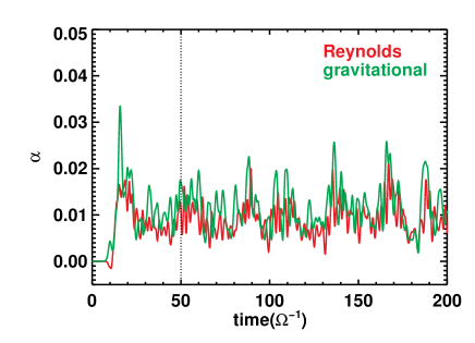
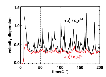
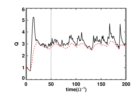
Figure 1: Time history of the gravito-turbulent disk of pure gas case with $t_{\rm{cool}}\Omega=10$. Top left: The gravitational (green) and Reynolds (red) stresses normalized with averaged pressure as a function of time. Top Right: the density dispersion versus time. Bottom left: the velocity dispersion with (red) and without (black) density weight. Bottom right: The averaged Toomre Q-parameter using sound speed with (red dashed) and without (black solid)density weight. In our dust+gas hybrid simulations, we choose $t=50\Omega^{-1}$ (indicated by vertical dotted lines) as our initial state and distribute dust particles randomly in space.

We start with pure gas simulations. At $t=0$ we initialize a uniformly distributed gas disk and set $\Sigma_{0}=\Omega=G=1$. The thermal energy is such that $Q=c_{\rm{s}}\Omega/(\pi G\Sigma_{0})=1.1$ close to the critical Toomre $Q$-parameter for a razor-thin disk ($\simeq 1$; Toomre, 1964; Goldreich & Lynden-Bell, 1965), where $c_{\rm{s}}=\sqrt{\Gamma(\Gamma-1)U/\Sigma}$ is the sound speed. The velocity is $\mathbf{u_{0}}=(\delta_{x},-q\Omega x+\delta_{y})$, where $\delta_{x}$ and $\delta_{y}$ are randomized perturbations at $\sim$$1\%$ of the initial sound speed $c_{\rm{s}}{{}_{0}=1.1\pi}$. Our simulation domain is a box which covers $[-80,80]\,G\Sigma_{0}/\Omega^{2}$ in both radial ($x$) and azimuthal ($y$) direction with $512^{2}$ grid points. This amounts to a spatial span of $160H/(\pi Q)\simeq 51Q^{-1}H$ and a resolution of $\simeq 10Q/H$, where $H\equiv c_{\rm{s}}/\Omega=\pi Q(G\Sigma_{0}/\Omega^{2})$ is the disk scale height.

We allow the disk to cool off immediately with a fixed cooling time $t_{\rm{cool}}\Omega\in\{5,10,20,40\}$. After a short transient phase which normally takes about twice the cooling time, the disk settles to a quasi-steady gravito-turbulent state in which the heating from compression and shocks is balanced by the imposed cell-by-cell cooling. For example, we show the time evolution of Reynolds and gravitational stresses, surface density and velocity dispersions and Toomre’s Q parameter from the $t_{\rm{cool}}\Omega=10$ case in Figure 1.

All quantities saturate after $\geq 20\Omega^{-1}$, and well established turbulence sustains to the end of the simulations (hundreds of dynamical times). The time averaged ($t>50\Omega^{-1}$) nominal $\alpha$, i.e., stresses normalized with pressure, is $\alpha\simeq 0.020$ for the sum of the Reynolds and gravitational stress. Toomre’s Q is hovering $\sim 3$ (Gammie, 2001) which also sets the spatial averaged sound speed $\langle c_{\rm{s}}\rangle=\pi Q(G\Sigma_{0}/\Omega)$. The Q-parameter using density weighted sound speed $\langle c_{\rm{s}}\rangle_{\scriptscriptstyle\Sigma}$ (red dashed curve in bottom right panel) shows less fluctuation and slightly diminished ($\sim 10\%$) mean. We choose the density weighted measure hereafter and simply use $\langle c_{\rm{s}}\rangle$ to represent the density weighted sound speed. But we do note that the spatial and temporal averaged velocity dispersion $\langle u_{\rm{x}}\rangle$ (black) is about twice the density weighted value $\langle u_{\rm{x}}\rangle_{\scriptscriptstyle\Sigma}$ (red) as shown in the bottom left panel of Figure 1. The cause and effects will be discussed in section 3.2. We also emphasize that the density dispersion $\delta\Sigma_{g}/\Sigma_{0}\simeq 0.6$ for $\alpha\sim 0.02$, much stronger than found in the MRI-driven turbulence case where $\delta\rho/\rho\sim\sqrt{0.5\alpha}\sim 0.1$ for similar $\alpha$ values with or without net weak magnetic field (Nelson & Gressel, 2010; Okuzumi & Hirose, 2011; Shi et al., 2016). We will discuss it further in section 3.7.

We then randomly distribute dust particles in space at $t=50\Omega^{-1}$ (for $t_{\rm{cool}}\Omega\leq 20$) or $100\Omega^{-1}$ (for $t_{\rm{cool}}\Omega=40$), and evolve the particle+fluid system for another $200\Omega^{-1}$. We implemented seven types of particles with constant stopping time such that the Stokes number $\tau_{s}\equiv\Omega t_{\rm{stop}}\in[10^{-3},10^{-2},0.1,1,10,10^{2},10^{3}]$, evenly spaced in logarithmic scale. For each type, we use $2^{19}$ ($\sim$$5\times 10^{5}$) particles, or $\sim$ 2 particles per grid cell on average. Their velocities follow the background shear initially. Since gas densities vary in time and space, it would be more physical to fix the size of each particle rather than its stopping time; nevertheless, our default simulations fix stopping times to more easily compare with previous simulations that do likewise. We also verify explicitly that our simulations with fixed stopping time agree well with a simulation that uses fixed particle sizes (see Section 3.6). For this latter run, we employ a stopping time based on the Epstein drag law:

$$t_{\rm{stop}}{{}_{,i}}=\frac{fa^{*}_{i}}{\Sigma c_{\rm{s}}}\,,$$ (9)

where $a^{*}_{i}=10^{i-4}$ for $i=1$–$7$ is the dimensionless size of the $i$-th particle species. The converting factor $f\simeq 3\pi(G\Sigma_{0}^{2}/\Omega^{2})$ is chosen such that $fa^{*}_{i}/\langle\!\langle\Sigma c_{\rm{s}}\rangle\!\rangle_{\rm t}\sim a^{*}_{i}$, matching $\tau_{s}$ used in the fixed stopping time runs.

3 RESULTS

3.1 Standard run

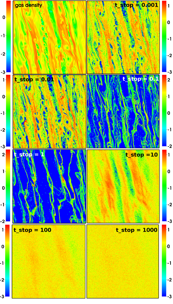
Figure 2: Snapshots of gas and dust surface density distributions at the end of simulation. The domain size is $L_{\rm{x}}=L_{\rm{y}}=160G\Sigma_{0}/\Omega^{2}\simeq 17H$, and cooling time is $10\Omega^{-1}$. Values are normalized against initial values and color coded in log scale. We see small $t_{\rm{stop}}$ particles tracing the gas; particles with intermediate $\tau_{s}=0.1$-$1$ strongly clustering; and larger particles diffused across the domain.

We first present our standard run tc=10, i.e., $t_{\rm{cool}}\Omega=10$ run (see Table 1 for the gas properties). After distributing the particles randomly on the grid, the particles quickly adjust in response to the dynamical gas flows. After $\sim 20\Omega^{-1}$, the distribution of particles reaches a steady state. As an illustration, we have shown the gas and dust density in Figure 2 at $t=180\Omega^{-1}$. Clearly, the small particles ($\tau_{s}\leq 10^{-2}$) are nearly perfectly coupled to the gas and therefore share the same density structures of the gas. Particles with intermediate stopping time, for both $\tau_{s}=0.1$ and $1$, appear to concentrate along the dense gas filaments and cause dust density enhancement of two orders of magnitude relative to the mean (note the color bars for $\tau_{s}=0.1$ and $1$ now extend to higher values). Transient vortices are also observable in the snapshots for gas and $\tau_{s}<1$ particles, but are probably under-resolved; see Gibbons et al. (2015) for the effects of vortices on particle concentration. For large particles ($\tau_{s}\geq 10$), they are strongly disturbed by the gravitational stirring from the fluctuating gas (see further discussion of the effects of gravity in section 3.5). After $\sim 20\Omega^{-1}$, they are completely redistributed and their end status recovers a random distribution similar to the initial.

In Figure 3, we show the time-averaged fraction of cumulative mass for each type of particle, binned in local surface density (number of particles in each cell) normalized to the mean ($2$/cell). The running profiles of small sized particles resemble that of the time-averaged gas (solid black curve). Those with large stopping times track the initial random distribution (dotted black). In contrast, the blue ($\tau_{s}=1$) and green ($\tau_{s}=0.1$) curves show that intermediate-sized particles exhibit relatively higher densities, $\Sigma_{p}/\langle\Sigma_{p}\rangle\sim 10$–$100$.

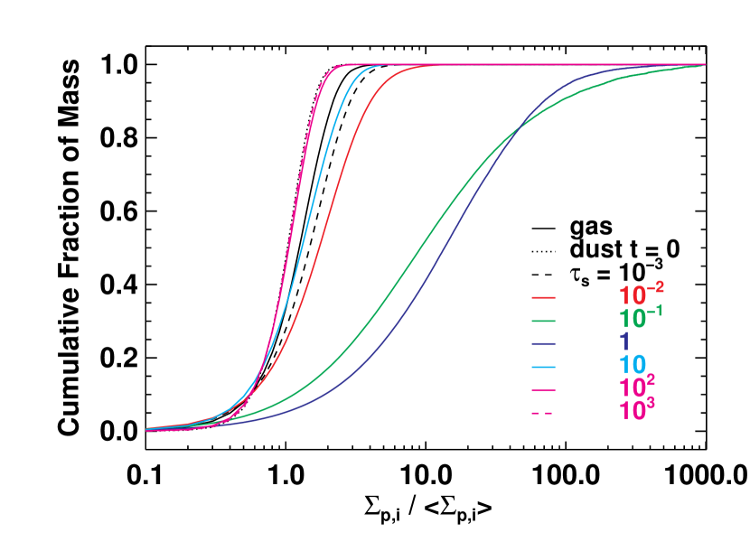
Figure 3: The time-averaged cumulative fraction of the total particle mass as a function of particle surface density. The surface density is normalized by the averaged value (equal to the initial value) and thus represents the concentration factor of the dust particles. We also show the time-averaged gas distribution (black solid) and the initial dust distribution (black dotted) for comparison.

After reaching quasi-steady state, we further evolve the dust+gas mixture for a total duration of $200\Omega^{-1}$. We then measure the radial diffusion coefficients, particle eccentricity and relative velocities averaged over all particles of the same type. The results are presented in the following subsections.

3.2 Radial diffusion

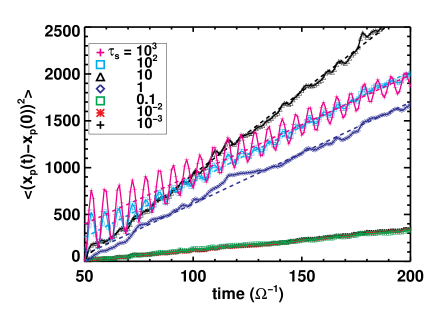
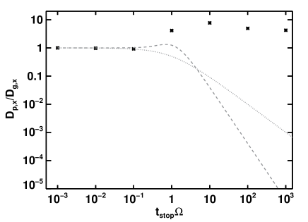
Figure 4: Left: The squared radial displacement versus time for all types of particles ($\tau_{s}\equiv t_{\rm{stop}}\Omega$) in run tc=10 ($t_{\rm{cool}}\Omega=10$. The color symbols (with solid curves) are measurement, the dashed curves are the linear fits to the data. Their slopes are then twice the diffusion coefficients based on Equation 10. Right: Symbols mark the radial diffusion coefficients for particles with different stopping time. At larger stopping time, the measured coefficients are largely different than models of either Youdin & Lithwick (2007) (dashed gray curve) or Cuzzi et al. (1993) (dotted) due to extra stirring from the gas self-gravity.

We utilize the following formula to derive the radial diffusion coefficients $D_{\rm{p,x}}$ of different types of particles in our simulations (Youdin & Lithwick, 2007; Carballido et al., 2011):

$$D_{\rm{p,x}}\equiv\frac{1}{2}\frac{d\langle|x_{p}(t)-x_{p}(0)|^{2}\rangle}{dt}\,,$$ (10)

where $D_{\rm{p,x}}$ is the diffusion coefficient for given particle stopping time, $x_{p}(t)$ and $x_{p}(0)$ are the radial position at time $t$ and initial (taken to be $50\Omega^{-1}$ after injecting the particles to the gas disk). The radial coordinate is extended beyond the edges of the sheet so that particles moves on radially without periodic boundary conditions. The measurements are made at every time interval $\delta t=0.5\Omega^{-1}$, and are performed for a duration of $150\Omega^{-1}$ long. The average $\langle\,\rangle$ here is taken for all particles within the same type.

The squared displacements as a function of time on the right hand side of Equation (10) are shown in the left panel of Figure 4. Each curve represents the displacement of one distinctive type of particles. For particles of $\tau_{s}\leq 0.1$, the curves overlap. As they are well-coupled with the turbulent gas flows, their displacements reflect the properties of gas diffusion. For larger particles, the gravitational stirring dominates the drag force which introduces some extra effective diffusion. As a result, the displacement curves of those particles have bigger slopes. For the largest two dust species we implemented, the curves show periodic oscillations which are due to the epicyclic motion of individual particles. The large amplitude of the epicyclic motion is a result of the strong gravitational forcing of the background gas.

Now with the help of Equation 10 and Figure 4, we can derive the radial diffusion coefficients based on the slope of the squared displacements using linear fitting. The results are shown in the right panel of Figure 4 and also recorded in Table 2. The radial diffusion coefficients $D_{\rm{p,x}}$ are normalized against the gas diffusion coefficient $D_{g,x}$; the latter is approximated using the $D_{\rm{p,x}}$ of particles with $\tau_{s}=10^{-3}$. We find $D_{\rm{p,x}}\simeq D_{\rm{g,x}}$ for $\tau_{s}\leq 0.1$. However, $D_{\rm{p,x}}$ exceeds $D_{\rm{g,x}}$ for particles with longer $t_{\rm{stop}}$, and stay roughly constant, $D_{\rm{p,x}}\sim 6$–$8D_{\rm{g,x}}$. For comparison, we also plot the diffusion coefficient predicted by models in Cuzzi et al. (1993, dotted gray curve) and Youdin & Lithwick (2007, dashed gray). Both predict small and decreasing values for larger particles based on homogeneous turbulence without extra forcing like self-gravity, in clear contrast with what we obtain in our gravito-turbulent disk. When gravitational stirring is artificially suppressed (see section 3.5), we do recover similar relationship as they predicted.

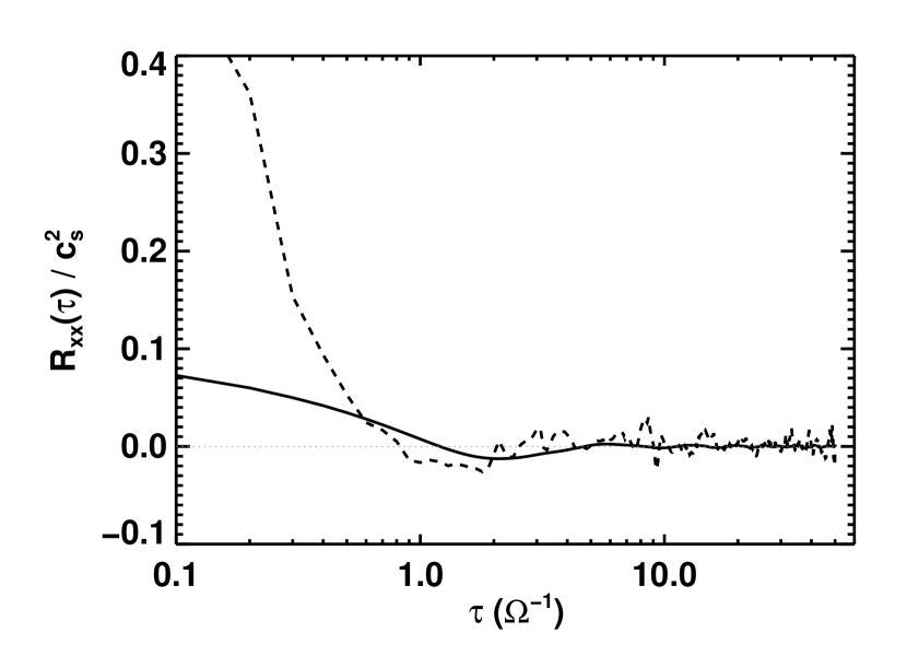
Figure 5: The radial velocity auto-correlation functions of the gravito-turbulent gas disk calculated with (solid) and without (dashed) density weight.

We also check the validity of approximating $D_{\rm{g,x}}$ with $D_{\rm{p,x}}$ by measuring the auto-correlation function of the turbulent velocity field directly. In general,

$$D_{\rm{g,x}}=\int_{0}^{\infty}R_{\rm xx}(\tau)d\tau\,,$$ (11)

where $R_{\rm xx}(\tau)=\langle u_{\rm{x}}(\tau)u_{\rm{x}}(0)\rangle$ is the auto-correlation of the gas velocity at time $\tau$. However, in gravito-turbulent disk, the spiral density shock waves cause low density ($\Sigma/\Sigma_{0}\sim O(10^{-2})$) valleys between high density ($\Sigma/\Sigma_{0}\sim O(1)$) ridges. Most of the matter in the high density regions has small velocity, but the gas in low density region has very high velocity ($\sim c_{\rm{s}}$). The auto-correlation function defined above would strongly bias toward the low density instead of the high density region where most of the small dust particles reside. One way to remove the bias is to calculate the gas or dust density weighted auto-correlation function

$$R_{\rm xx}(\tau)=\frac{\int\!\Sigma(\tau)u_{\rm{x}}(\tau)\Sigma(0)u_{\rm{x}}(0)dxdy}{\int\!\Sigma(\tau)\Sigma(0)dxdy}=\langle u_{\rm{x}}(\tau)u_{\rm{x}}(0)\rangle_{\scriptscriptstyle\Sigma}\,,$$ (12)

in which $u_{\rm{x}}(0)$ and $\Sigma(0)$ are velocity and density at a reference time, $u_{\rm{x}}(\tau)$ and $\Sigma(\tau)$ are measured at time $\tau$ from the reference point and are both sheared back to that point in order to calculate the correlation. Shown in Figure 5 is the velocity auto-correlation calculated with (solid curve) and without (dashed curve) density weight. Integrating the density weighted $R_{\rm xx}$, we get $D_{\rm{g,x}}\simeq 0.014\langle\!\langle c_{\rm{s}}\rangle\rangle\Omega^{-1}$ close to the $D_{\rm{p,x}}\simeq 0.012\langle\!\langle c_{\rm{s}}\rangle\rangle\Omega^{-1}$ measured with particles of $\tau_{s}=10^{-3}$. However, using $R_{xx}$ without density weight would overestimate the diffusion coefficient by a factor of $15$.

3.3 Eccentricity growth

When particle eccentricity is small, we have the relation

$$v_{\rm{x}}^{2}\simeq 2v_{\rm{y}}^{2}\simeq e^{2}\Omega^{2}r^{2}\,.$$ (13)

We can therefore measure the orbital eccentricity of each individual particle according to this relation, and obtain the evolution of the eccentricity as shown in Figure 6. Although the initial $e=0$, we find the mean eccentricity quickly saturates at $e\simeq 0.2$-$0.3(H/R)$ for particles of $\tau_{s}\leq 1$. It then saturates slower and levels off at greater value for increasing $\tau_{s}>1$. The saturated values are $e\simeq 0.7(H/R)$ and $1.3(H/R)$ for $\tau_{s}=10$ and $10^{2}$ particles (see Figure 7). The eccentricity of $\tau_{s}=10^{3}$ particle keeps rising gradually through the end of the simulation, suggesting that a saturation level of $\gtrsim 2(H/r)$ might be achieved for a longer simulation which is consistent with previous simulations of planetesimals in gravito-turbulent disks (Britsch et al., 2008; Walmswell et al., 2013). We also find that the particle eccentricity obtained in gravito-turbulent disk is in general much greater than that could be excited in the MRI-driven turbulent disk with similar turbulent stress-to-pressure ratio $\alpha$. The latter usually gives $e\sim 10^{-2}$–$10^{-1}(H/R)Q^{-1}$ (Yang et al., 2009, 2012; Nelson & Gressel, 2010), orders of magnitude smaller than what we have observed here in our simulations.

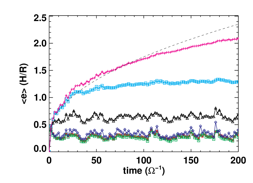
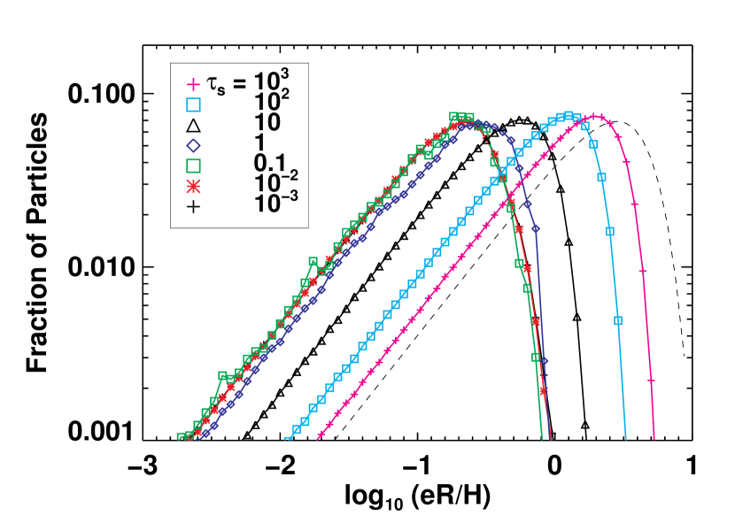
Figure 6: Top: The time evolution of orbital eccentricities averaged over all particles of the same type. The dashed line is $0.15(\Omega t)^{1/2}$, which characterize the early growth of the eccentricity for large particles. Bottom: The relative number distribution of particle eccentricity at late time of simulation. We choose 100 bins evenly divided between $\log_{10}(eR/H)=-3$ and $1$ for the distribution plot. The dashed line shows a typical Rayleigh distribution for comparison.

Since the particle eccentricity is excited by nearly random gravity field, the evolution will follow the general $\propto\sqrt{t}$ law (Ogihara et al., 2007),

$$e=C\left(\frac{H}{R}\right)(\Omega t)^{1/2}\,,$$ (14)

where the dimensionless coefficient $C$ determines the growth rate and can be measured with our simulation. We fit the early growing phase of the both $\tau_{s}=10^{2}$ (cyan square) and $10^{3}$ (magenta cross) with the above relation and obtain $C\simeq 0.15$ as the best fit coefficient (see the black dashed curve in Figure 6) The excitation time scale of eccentricity could be estimated as $t_{\rm exc}\sim e/(de/dt)\sim 2e^{2}(R/H)^{2}C^{-2}\Omega^{-1}$. We can therefore predict the saturated eccentricity by equating $t_{\rm exc}$ with the damping time scale, in our case, is simply the stopping time $t_{\rm{stop}}$. The eccentricity at saturation is therefore

$$e\sim C(H/R)(\tau_{s}/2)^{1/2}\,.$$ (15)

For $\tau_{s}=10^{2}$ particles, this gives $e\sim 1.1(H/R)$ that matches what we observe in Figure 6 very well. It also predicts a saturation level of $e\sim 4.7(H/R)$ if we extend the simulation for another $\sim 300\Omega^{-1}$.

Equation 14 also allows us to measure the dimensionless parameter $\gamma$ which characterizes the amplitude of the fluctuating gravity field as defined in Ogihara et al. (2007). Following Ida et al. (2008) and Okuzumi & Ormel (2013), we write the eccentricity growth as

$$e\simeq 1.6\gamma\left(\frac{M_{\odot}}{M_{*}}\right)\left(\frac{\Sigma}{10\,{\rm g}\,{\rm cm^{-3}}}\right)\left(\frac{R}{100\,{\rm AU}}\right)^{2}\left(\Omega t\right)^{1/2}\,.$$ (16)

After comparing with Equation 14, we find the dimensionless turbulent strength $\gamma\simeq 0.01$ in our gravito-turbulent disk with $\Omega t_{\rm{cool}}=10$ or $\alpha\simeq 0.02$, considerably larger than that in MRI disks with similar $\alpha$ (e.g., $\gamma\sim 10^{-4}$ in Yang et al., 2012).

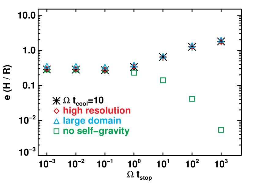
Figure 7: The time averaged (last $15$ orbits) particle eccentricity (or equivalently the velocity dispersion $\delta v/c_{\rm{s}}$) varies with stopping time. The standard run using $t_{\rm{cool}}=10\Omega^{-1}$ are shown in asterisk. The label ‘high resolution’, ‘large domain’, and ‘no self-gravity’ represent results from tc=10.hires using doubled resolution, tc=10.dble with doubled sheet size, and tc=10.wosg without gravitational forcing from the gas respectively, and are discussed in section 3.5 and 3.8.

We also calculate the saturated eccentricity distributions of particles. In Figure 6, we find that particles of all types obey a Rayleigh-like distribution (Yang et al., 2009, 2012). The probability rises toward greater eccentricity, and then drops at roughly the mean eccentricity measured in the top panel of Figure 6. Particles having $\tau_{s}<1$ share nearly the same properties as gas. As $\tau_{s}$ increases above unity, increasingly many particles obtain higher eccentricities owing to stochastic gravitational forcing by gas. This behavior contrasts with that shown in Figure $6$ of Gibbons et al. (2012), in which the particle velocity distribution narrows as $\tau_{s}$ exceeds unity; their simulations omit gravitational stirring.

3.4 Relative velocity

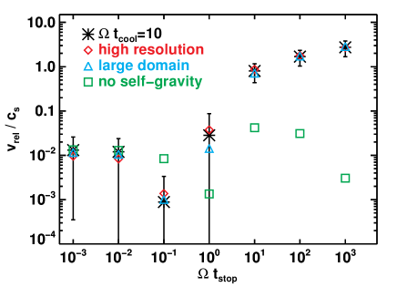
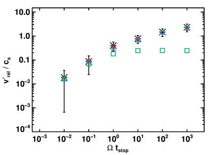
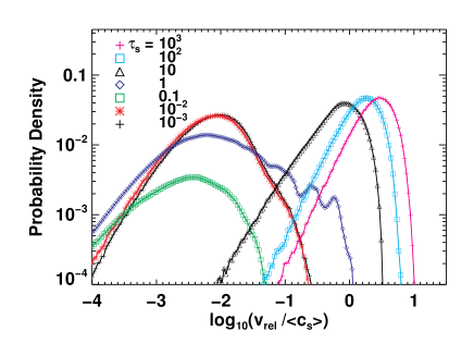
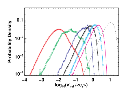
Figure 8: Average relative velocities versus particle stopping time (top row), and underlying probability density distributions of relative velocity (bottom row). Averages are taken over the final orbit of the simulations. The relative velocity $v_{\rm rel}$ is evaluated between particles of the same type (stopping time), while $v^{\prime}_{\rm rel}$ is measured with respect to $\tau_{s}=10^{-3}$ particles. Error bars show the standard deviation for run tc=10 alone (asterisks). The probability density curve for $v_{\rm rel}$ between $\tau_{s}=0.1$ particles (green squares in bottom left panel) has a diminished amplitude because there is significant probability at $v_{\rm rel}/\langle c_{\rm{s}}\rangle<10^{-4}$, which is off the scale of the plot. For comparison, a Maxwellian distribution is shown in the bottom right panel as a dashed curve.

The high eccentricities obtained in these particles indicate large velocity dispersion, which leads to the question of what is the relative velocity between pair collision. We thus measure the relative velocity of the same type particle or the mono-disperse case $v_{\rm rel}$, and also the relative velocity with respect to the smallest grains ($\tau_{s}=10^{-3}$) or a bi-disperse velocity $v_{\rm rel}^{\prime}$, in each grid cell assuming there is no sub-structure below this scale. The results are shown in Figure 8.

In general, the relative velocity (see the asterisk symbols in top two panels) $v_{\rm rel}$ and $v_{\rm rel}^{\prime}$ increase from $\sim 10^{-2}c_{\rm{s}}$ to $\gtrsim c_{\rm{s}}$ as the $\tau_{s}$ increases from $10^{-3}$ to $10^{3}$ which is indicated by the increasing velocity dispersion or eccentricity as discussed in previous section. Exceptions occur at $\tau_{s}=0.1\rm{-}1$, where particles show the strongest clustering effects (coherent and therefore less relative motions in the filaments), the relative velocity of the same type particles is largely reduced. It even drops below $10^{-3}c_{\rm{s}}$ for $\tau_{s}=0.1$ case. The general approach of approximating particle relative velocity via the measurement of velocity dispersion fails here. Our $v_{\rm rel}$ and $v_{\rm rel}^{\prime}$ for smaller particles ($\tau_{s}\leq 0.1$) seem similar to what are found in MRI-driven turbulent disks (Carballido et al., 2010). However, our $v_{\rm rel}$ and $v^{\prime}_{\rm rel}$ increases with $t_{\rm{stop}}$ for larger particles that have $\tau_{s}>0.1$, in contrast to MRI-driven turbulence results (c.f. Figure 2 and 3 in Carballido et al., 2010) where turbulent torquing due to the fluctuating gravity field of the gas is not considered. The latter show $v_{\rm rel}$ falls continuously, and $v^{\prime}_{\rm rel}$ stays roughly constant with $t_{\rm{stop}}$, in agreement with the theoretical prediction in isotropic turbulence (Ormel & Cuzzi, 2007). We will discuss the effects of gravitational stirring in section 3.5.

We also show the probability density functions (PDFs) for $v_{\rm rel}$ and $v_{\rm rel}^{\prime}$ in Figure 8. The PDFs of larger particles ($\tau_{s}>1$) are similar to Maxwellian distribution (see the dashed curve in the bottom right panel as an example of Maxwellian distribution) (Windmark et al., 2012; Garaud et al., 2013). Particles smaller than $\tau_{s}\sim 1$, however, show broader distributions and smaller mean values than the bigger particles. They deviate significantly from a Maxwellian and resemble more of a log-normal distribution (Mitra et al., 2013; Pan et al., 2014). Relative velocities with respect to the smallest particles, i.e., $v^{\prime}_{\rm rel}$, have distributions that shift gradually to higher values as the size of the larger particle increases. Between $\tau_{s}=0.01$ and $\tau_{s}=0.001$ particles, the largest relative velocities $v^{\prime}_{\rm rel}>0.1c_{\rm{s}}$, which might lead to collisional destruction, are mostly due to their different deceleration rates in post-shock regions (Nakamoto & Miura, 2004; Jacquet & Thompson, 2014). As plotted in Figure 9, the locations where $v^{\prime}_{\rm rel}>0.1c_{\rm{s}}$ (white symbols) are found just behind shock fronts, where gas radial velocities are discontinuous.

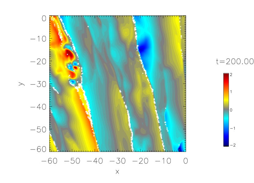
Figure 9: Snapshot of gas radial velocities (normalized by the volume-averaged sound speed) at $t=200\Omega^{-1}$. Large relative velocities ($>0.1c_{\rm{s}}$) between $\tau_{s}=10^{-2}$ and $10^{-3}$ particles are overlaid as white symbols. Evidently, large relative velocities between particles characterize regions just behind shock fronts; in post-shock regions, particles decelerate at different rates according to their different stopping times (Nakamoto & Miura, 2004; Jacquet & Thompson, 2014).

Relative velocities $v_{\rm rel}$ between particles of the same type can be separated into two groups. One group corresponds to the small-size particles ($\tau_{s}\leq 1$), for which relative velocities peak at $v_{\rm rel}\simeq 0.01c_{\rm{s}}$. The other group corresponds to large-sized particles ($\tau_{s}>1$), for which peak velocities are sonic. We note that $\tau_{s}=0.1$ (green squares) particles show diminished amplitude and a significant shift toward smaller relative velocity due to the clustering effect: $\sim 80\%$ of contribution from $v_{\rm rel}/c_{\rm{s}}\ll 10^{-4}$ is not shown in this plot. While for $\tau_{s}=1$ particles, there is also a second, near sonic, contribution, which shows the transitional behavior from small size (friction-dominated) to large size (gravity-dominated) particles.

3.5 Effects of gravitational stirring

The gravitational stirring effect has been studied in MRI-driven turbulent disks and shown to induce high velocity dispersion for solid bodies bigger than $\sim 100\,\rm{m}$ (or $\tau_{s}\gtrsim 10^{3}$ at radius $R\sim$ AU) (Nelson & Gressel, 2010; Yang et al., 2009, 2012; Okuzumi & Ormel, 2013; Ormel & Okuzumi, 2013). But we will show the dominating gravitational forcing kicks in for even smaller particles owning to its much stronger density fluctuation, $\delta\Sigma/\Sigma\sim 5\sqrt{\alpha}$ in gravito-turbulent disks (see section 3.7) rather than $\sim\sqrt{0.5\alpha}$ in MRI-driven turbulent disks (Nelson & Gressel, 2010; Yang et al., 2012).

As the stopping time increases, the first term in Equation (8), the drag force, becomes less important compared to the second term, the gravitational acceleration. Assuming the characteristic length scale of the spiral density features is $l$, then $|\nabla\Phi|\sim\Phi/l\sim G\delta\Sigma$, where $\delta\Sigma\sim\Sigma$ in our gravito-turbulent disk is the density fluctuation. The length scale can be approximated with the most unstable wavelength for axisymmetric disturbances, or simply the disk scaleheight, $l\sim c_{\rm{s}}^{2}/G\Sigma\sim Q^{2}(G\Sigma/\Omega^{2})\sim H$. This is also supported by our simulations; the density waves have typical radial wavelength $\sim H$ in the top left panel of Figure 2. The drag force $|u_{\rm{x}}-v_{\rm{x}}|/t_{\rm{stop}}\lesssim\Omega l/t_{\rm{stop}}\sim c_{\rm{s}}/t_{\rm{stop}}$. The ratio of these two thus gives

$$\frac{|\nabla\Phi|}{|u_{\rm{x}}-v_{\rm{x}}|/t_{\rm{stop}}}\sim\frac{1}{Q}\frac{\delta\Sigma}{\Sigma}\tau_{s}\,,$$ (17)

the gravitational stirring becomes more important than aerodynamical drag when $\tau_{s}>Q\sim 1$ in gravito-turbulent disks. However, for non-self-gravitating turbulent disks such as MRI-driven turbulent disks, $\delta\Sigma/\Sigma$ is one order of magnitude smaller, and $Q\gg 1$. As a results, the gravitational stirring only affect particles with $\tau_{s}>10Q\gg 1$.

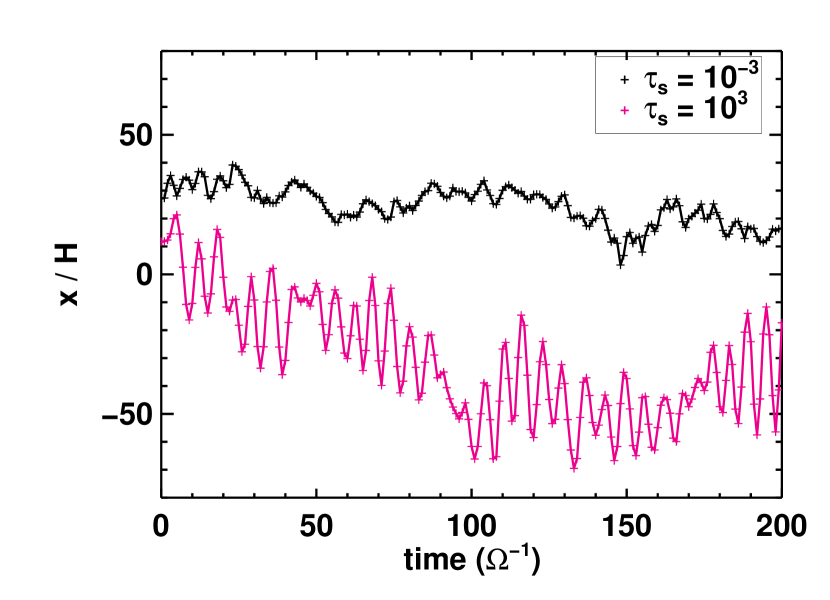
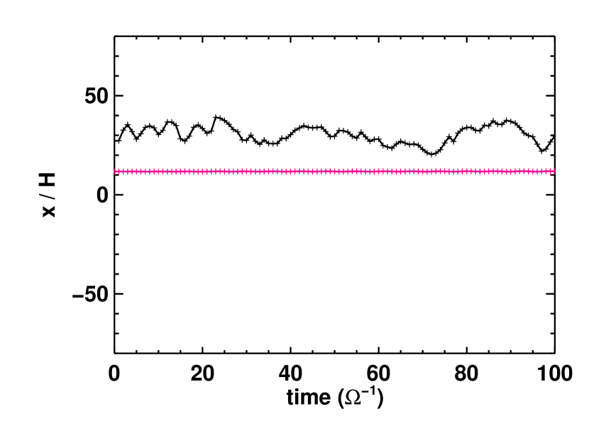
Figure 10: Examples of radial displacement for two particles with fixed stopping time $\tau_{s}=10^{-3}$ (black) and $10^{3}$ (magenta) in run with (top panel) and without (bottom panel) gravity pull from the gas in the calculation. The gravitational stirring of the $\tau_{s}=10^{3}$ particle causes large amplitude oscillations which are absent in the bottom panel when gravity from the gas is removed.

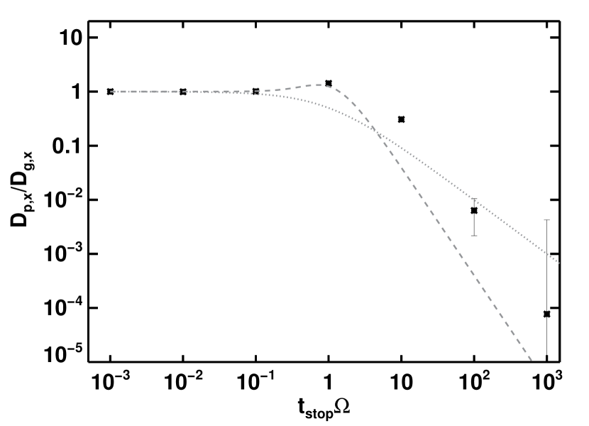
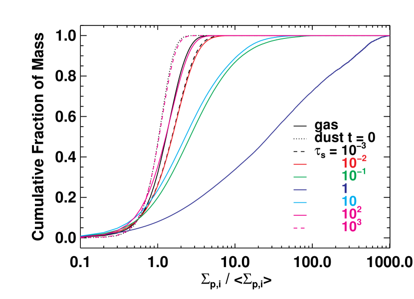
Figure 11: Similar to Figure 4 and 3, we show radial diffusion coefficients (top panel) and cumulative fraction of dust mass (bottom panel) for run tc=10.wosg, in which the gravitational forcing from the gas is artificially removed. At larger stopping time, the measured $D_{\rm{p,x}}$ without gravitational stirring are now closer to models of Youdin & Lithwick (2007) (dashed gray curve) or Cuzzi et al. (1993) (dotted). The clustering effect for particles of $\tau_{s}=0.1$ observed in Figure 3 is absent when gravitational stirring is removed.

In top panel of Figure 10, we show the time variation of radial positions of two representative particles in the standard simulation. The particle with larger $\tau_{s}=10^{3}$ oscillates with a peak-to-peak amplitude of $\sim 40G\Sigma_{0}/\Omega^{2}$ at a frequency of the orbital frequency $\Omega$ after it is released in the turbulent disk. However, the small particle, $\tau_{s}=10^{-3}$, scatters randomly over time and does not show strong periodic variations.

To reveal the self-gravity effect to the dust dynamics, we perform a rerun (tc=10.wosg) of the standard simulation but suppress the gravitational forcing manually, i.e. removing $-\nabla\Phi$ term in Equation 8. The radially projected trajectories of the same two representative particles are plotted in the bottom panel of Figure 10 for comparison. Clearly, the small particle is not affected by the missing of gravitational acceleration, and appears to behave similarly as in the standard run. However, the larger particle in tc=10.wosg barely moves radially when the only acceleration/deceleration is friction.

Without the gravitational stirring, the diffusion of particle also look significantly different than in Figure 4. In Figure 11, we present the diffusion coefficients measured in run tc=10.wosg using the same method as in Figure 4. Again, the small $t_{\rm{stop}}$ particles are unaffected and therefore give nearly the same $D_{\rm{p,x}}$ as in the standard run. $D_{\rm{p,x}}$ of particles with $\tau_{s}>1$ drops rapidly as $D_{\rm{p,x}}\propto(\tau_{s})^{-2}$ which manifests the lack of gravitational forcing. We note the exact relation between diffusion coefficient and stopping time slightly deviates from models of Cuzzi et al. (1993); Youdin & Lithwick (2007). We speculate that is a result of different power spectra in gravito-turbulent disks than normal homogeneous turbulence model adopted in these models.

In Figure 11, we also compute the cumulative mass fraction for run tc=10.wosg. As expected, the $\Omega t_{\rm{stop}}=1$ particles show the strongest concentration and more contribution towards the higher concentration ($\gtrsim 100$) than the standard tc=10 run. Both $\Omega t_{\rm{stop}}=0.1$ and $\Omega t_{\rm{stop}}=10.0$ show similar secondary clustering but are much weaker than the concentration of $\Omega t_{\rm{stop}}=0.1$ in the case where gravity is present.

Without the stochastic gravitational stirring, the averaged particle eccentricity for all types of particles never exceed $e\sim 0.3(H/R)$ as shown in Figure 7 (green squares). The small particles ($\tau_{s}\leq 1$) have similar eccentricities as in the standard run; however, those larger particles are dynamically unimportant, and $e$ approaches nearly zero (initial value) as $\tau_{s}$ increases. The gravitational stirring is also responsible for the increasing relative velocities for particles of $\tau_{s}\geq 1$. As shown in top row of Figure 8 in green squares, instead of rising up, $v_{\rm rel}$ decreases while $v^{\prime}_{\rm rel}$ stays constant with increasing $\tau_{s}$ when gravitational forcing is not included, which is consistent with the results from previous study (Ormel & Cuzzi, 2007; Carballido et al., 2010).

3.6 Fixed particle size

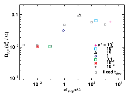
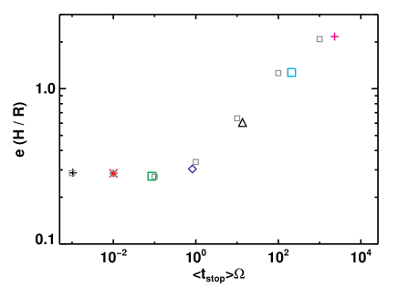
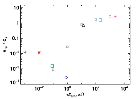
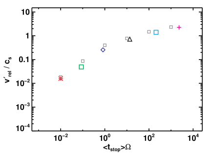
Figure 12: Diffusion coefficients (top left), particle eccentricity (top right), relative velocities $v_{\rm rel}$ (bottom left) and $v^{\prime}_{\rm rel}$ (bottom right) versus the effective stopping time for fixed size simulation tc=10.size. The effective stopping times are calculated by time and particle averaging of $t_{\rm{stop}}$ of individual particle. Results of tc=10 from Figure 4, which are shown with smaller grey squares, almost match fixed size results and therefore validate the usage of fixed stopping time particles in this work. We note the constant $t_{\rm{stop}}$ approach could overestimate the relative speed for intermediate size particles with $a^{*}=1$ or effective $\tau_{s}\sim 1$.

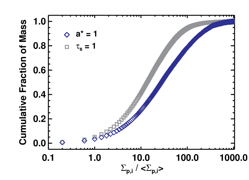
Figure 13: How particles concentrate in a run with fixed stopping time $\tau_{s}=1$ (from run tc=10) versus a run with fixed particle size $a^{*}=1$ (from run tc=10.size). The latter case, having an effective $\tau_{s}\simeq 0.83$, shows stronger concentration.

In case that the fluctuations of the density and sound speed are large ($\lesssim O(1)$), as is the case in gravito-turbulent disks, the constant stopping time assumption for individual particles might not be valid as the particles would have varying $t_{\rm{stop}}$ as they travel around different regions of the disk. We therefore, in this section, test if our results still hold statistically when we fix particle size instead of the stopping time.

We set up seven types of particles with fixed size, dimensionless size $a_{i}^{*}=10^{i-4}$ for $i=1$-$7$, as described in Equation (9) and section 2.2. Everything else is kept the same as the standard run tc=10. For each type of particles, we define an effective stopping time $\langle\langle t_{\rm{stop}}{{}_{,i}}\rangle_{\scriptscriptstyle\Sigma}\rangle_{t}$ by first measuring the stopping time of individual particle according to Equation 9, and then averaging over all particles of the same type and time. We find the averaged stopping time $\langle\langle\tau_{s}{{}_{,i}}\rangle\rangle_{t}\Omega\simeq[1.04\times 10^{-3},1.01\times 10^{-2},0.086,0.827,13.5,2.10\times 10^{2},2.31\times 10^{3}]$ for $a_{i}^{*}=10^{-3}$–$10^{3}$. For small particles ($a_{i}^{*}<0.1$), $\langle\langle\tau_{s}{{}_{,i}}\rangle\rangle_{t}\simeq a_{i}^{*}\Omega^{-1}$ as designed because we choose the converting factor$f$ in Equation 9 to match $a^{*}$ with $\tau_{s}$ of the fixed stopping time case. For intermediate size, the averaged stopping time is only $\lesssim 20\%$ smaller than the designed values. For larger particle with $a_{i}^{*}>1$, the effective stopping time is roughly $\sim 2a_{i}^{*}\Omega^{-1}$.

After converting $a^{*}$ to the effective stopping time, we find the results stay the same as the simulations using particles of constant stopping times. In Figure 12, we show the diffusion coefficient, particle eccentricity, and relative velocities in large colored symbols. They almost follow the results using fixed $t_{\rm{stop}}$ (gray squares). Therefore, statistically, these results validate the usage of fixed $t_{\rm{stop}}$ particles even in the highly fluctuated density field of a gravito-turbulent disk. In general, the results of fixed $t_{\rm{stop}}$ can approximate the results of fixed size particles. But this approach (constant $t_{\rm{stop}}$) might underestimate the clustering effect for the intermediate size particle $\tau_{s}=1$ as shown in Figure 13. This also leads to an overestimate of the relative speed $v_{\rm rel}$ for intermediate size particles of $\tau_{s}\sim 1$. The actual relative speed for intermediate size particles would become even smaller than what we have obtained.

3.7 Effects of cooling time

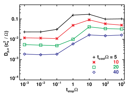
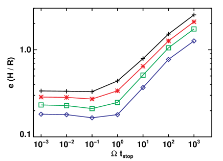
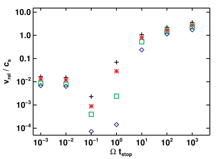
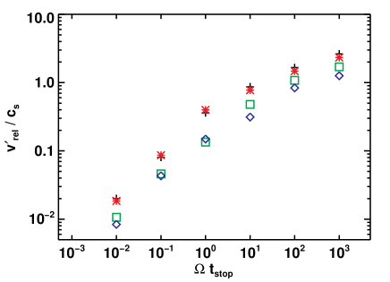
Figure 14: The dependence on cooling time (different symbols) of the radial diffusion coefficient (top left), saturated particle eccentricity (top right), relative velocity between particles of the same type (bottom left), and relative velocity with respect to $\tau_{s}=10^{-3}$ particles (bottom right). The measured $D_{\rm{p,x}}$ is nearly inversely proportional to $t_{\rm{cool}}$, while particle eccentricity and relative velocities roughly follow $t_{\rm{cool}}^{-1/2}$.

The dust dynamics would also be affected by the strength of the turbulence. In a gravito-turblent disk, the strength of the turbulence, e.g., in term of $\alpha$, is inversely proportional to the cooling time (Gammie, 2001; Shi & Chiang, 2014). We can therefore study how the dust dynamics changes with the turbulent strength by varying $t_{\rm{cool}}$.

We perform simulations with $t_{\rm{cool}}\Omega=5$ (run tc=5), $20$ (run tc=20), and $40$ (run tc=40) using the same particle distribution as in the $t_{\rm{cool}}\Omega=10$ standard run. We then measure the diffusion coefficient in each $t_{\rm{cool}}$ case and present the results in Figure 14. We find $D_{\rm{p,x}}$ of various cooling time share rather similar profile. It is flat at $\tau_{s}<0.1$ end when aerodynamical coupling is strong. $D_{\rm{p,x}}$ traces $D_{\rm{g,x}}$ in this regime, and the Schmidt number, which measures the ratio of angular momentum transport and mass diffusion, ${\rm Sc}\equiv\alpha c_{\rm{s}}^{2}\Omega^{-1}/D_{\rm{g,x}}\sim 1.4$–$2.4$, stays roughly constant. The diffusion coefficient rises up for $0.1\leq\tau_{s}\leq 1$, indicating the increasing effect of the gravitational stirring. In the very long stopping time regime, $\tau_{s}\geq 10$, the profile levels off again as the dominant gravitational acceleration does not depend on $t_{\rm{stop}}$. The magnitude of $D_{\rm{p,x}}$ is usually $5$–$9$ times of the diffusion of small particle or gas. For given particle size, we find $D_{\rm{p,x}}$ scales roughly as $\propto 1/t_{\rm{cool}}$ which indicates stronger diffusion in stronger turbulence.

Varying the cooling time also affects the particle concentration. In Figure 15, we show the density snapshots of simulations using different cooling times at the top row. As $t_{\rm{cool}}$ gets longer, we find the turbulent amplitude diminishes, so does the tilt angle of the shearing wave features. This leads to less frequent interactions between separated shearing waves and longer life time for existing density features. In the bottom row of Figure 15, we find strong interactions of shearing waves in $\Omega t_{\rm{cool}}=5$ run leads to plume-like structure of $\tau_{s}=1$ particle with typical concentration of $\sim 10$-$100$. The concentration is greater, $\gtrsim 100-10^{3}$ for $\Omega t_{\rm{cool}}=40$ case, and particles are more spatially confined in very narrow streams. In Figure 16, we quantitatively confirm this result by showing the cumulative mass fraction of the $\tau_{s}=1$ particles for various cooling times. As $t_{\rm{cool}}$ rises, more and more mass actually concentrate towards larger dust density, although the density dispersion of gas decreases.

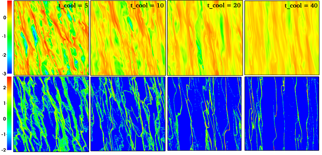
Figure 15: The logarithmic values of the gas (top) and $\Omega t_{\rm{stop}}=1$ particle density (bottom) at the end of simulations with various cooling time as shown in the top panels of each column. Color bars are on the left of each row. As $t_{\rm{cool}}$ increases, the fluctuation of gas density becomes weaker, the tilt angle of shearing waves also gets smaller, both indicates relatively weaker angular momentum transport as the cooling time scale gets longer. However, stronger clustering effects are found for longer cooling cases as the velocity dispersion from the gas gets weaker.

The particle relative velocity and eccentricity drops as the cooling time gets longer (see Figure 14). In general, from $\Omega t_{\rm{cool}}=10$ to $40$, $v_{\rm rel}$, $v^{\prime}_{\rm rel}$ and $e$ diminish by less than a factor of $\sim 2$-$3$, roughly scales as $\propto\alpha^{1/2}$, similar to the way velocity/density dispersion scales. Exceptions occur at the intermediate size particles (as found in section 3.4), $\tau_{s}=0.1$ and $1$, where we find the relative velocity of the same kind $v_{\rm rel}$ drops rapidly with increasing cooling time. It diminishes $\sim 30$ times from $\Omega t_{\rm{cool}}=5$ to $40$ for $\tau_{s}=0.1$ particles and $\lesssim 10^{3}$ times for particles with $\tau_{s}=1$. As the intermediate-sized particles show the strongest clustering, the rather slow relative velocity would favor gravitational collapsing.

Based on our results in Table 1, the density dispersion usually follows $\delta\Sigma/\Sigma\simeq 2(\Omega t_{\rm{cool}})^{-1/2}\simeq 5\alpha^{1/2}$ in gravito-turbulent disks. As already mentioned in section 3.5, this is much stronger fluctuation than found in MRI disks ($\sim\lesssim\alpha^{1/2}$). Similar as in section 3.3, we also measure the dimensionless turbulent strength $\gamma$ based on the eccentricity growth for different $t_{\rm{cool}}$ runs and list them in Table 1. The strength parameter $\gamma\simeq 0.07\alpha^{1/2}$ seems about one order of magnitude greater than those found in MRI-driven turbulent disks (Nelson & Gressel, 2010; Yang et al., 2012) which also explains why we observe much larger eccentricity and relative speed for large particles ($\tau_{s}>1$) in our gravito-turbulent disks.

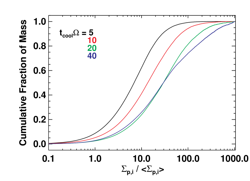
Figure 16: Similar to Figure 3, the cumulative mass fraction of the particles with $\Omega t_{\rm{stop}}=1$ for various cooling times. Longer $t_{\rm{cool}}$ results in stronger concentration and clustering.

3.8 Domain size and resolution effects

In this section, we investigate if our results are affected by the size of the computational domain we adopt. By doubling the size of the shearing sheet and meanwhile keeping the numerical resolution the same, run tc=10.dble quadruples the numbers of grid cells and dust particles. Following the discussion in section 2.2, we first start with a pure gas simulation with $\Omega t_{\rm{cool}}=10$ using now an extended domain. This simulation runs for $\sim 200\Omega^{-1}$ and quasi-steady gravito-turbulent stage is confirmed after $\lesssim 20\Omega^{-1}$. We then inject the particles at $t=50\Omega^{-1}$ similar to our standard run, and rerun for another $200\Omega^{-1}$ with now both gas and particles on the grids. The results are summarized in Table 1 (for the gas) and 2 (for the dust diffusion).

We find the gas properties of tc=10.dble, do not deviate much from those of the standard run tc=10. The diffusion coefficients for different type of dust particles are also very similar, $\sim 20\%$ of difference at most. No significant variations are observed comparing the particle eccentricity/relative velocities between the standard (black asterisk) and the double-sized (cyan triangles) simulations in Figure 7 and 8 either. We find similar clustering for the intermediate size particles as well. All these suggest converging results are obtained by adopting domain size of our standard run.

In another run tc=10.hires, we double the number of grid cells in $x$ and $y$ directions and quadruple the total numbers of particles for each species to study the effects of numerical resolution. The gas properties and the radial diffusion coefficients in this higher resolution run are listed in Table 2. We find doubling the resolution would slightly increase $\alpha_{\rm tot}$ and $D_{\rm{p,x}}$ by $\lesssim 20\%$. The particle eccentricity and relative velocities (see red diamond symbols in Figure 7 and top two panels of Figure 8) are also very similar to those from the standard run. We therefore confirm good numerical convergence in our results.

4 DISCUSSION

In this section, we try to construct a model of gravito-turbulent disk, and convert our scale free results in previous sections into a more physical and realistic format. An optically thin turbulent flow driven by gravity of its own can be easily found on the outskirts of protoplanetary disks. At an orbital distance of $R\sim 100$AU from a solar-mass star, a disk mass of $\Sigma R^{2}\sim 0.01M_{\odot}$ or surface density of $\Sigma\sim 10\rm{g}\,\rm{cm}^{-2}$, and a temperature of $T\sim 10\rm{K}$ would lead to a Toomre Q about unity and a cooling time scale much longer than the local dynamical time. Depending on the dust opacity of the disk, the cooling time can vary from several times to orders of magnitude longer than the local $\Omega^{-1}$ (Shi & Chiang, 2014). In this disk, $H/R\sim 0.1$ and gas density $\rho_{\rm g}\sim\Sigma/H\sim 10^{-13}\rm{g}\,\rm{cm^{-3}}$.

4.1 Particle sizes

The mean free path of the gas at radius $R\sim 100$AU is $\lambda\sim 10^{4}\rm{cm}$, which is typically much greater than the dust particle size we have simulated. Therefore the particle’s stopping time can be characterized as

$$\tau_{s}\simeq 0.1\left(\frac{s}{\rm{cm}}\right)\left(\frac{R}{100\,\rm{AU}}\right)^{-3/2}\left(\frac{T}{10\,\rm{K}}\right)^{-1/2}$$

$$\times\left(\frac{\rho_{s}}{1\,\rm{g\,cm^{-3}}}\right)\left(\frac{\rho_{g}}{10^{-13}\,\rm{g\,cm^{-3}}}\right)^{-1}\,,$$ (18)

using the Epstein’s law, where $s$ is the physical size of the dust particle. Specifically in our simulations, particles with $\tau_{s}=10^{-3}$ would be translated to $0.1$ mm in particle size, and $\tau_{s}=10^{3}$ corresponds to $0.1$ km planetesimals.

For particles even smaller than $0.1$ mm, they are perfectly coupled with gas, and will behave very similarly as the sub-mm-sized particles we explored using our simulations. For planetesimals even bigger than $0.1$ km in size, the stopping time starts to depend on the relative velocity between the dust and gas. However, similar to Equation 17, we can show that in the Stokes regime, the gravitational stirring always dominates the gas drag in our gravito-turbulent disk. The general empirical formula for the drag force reads $F_{\rm D}=0.5C_{\rm D}({\rm{Re}})\pi s^{2}\rho_{g}{\rm v_{gs}^{2}}$, where $\rm{Re}\sim s\rm{v_{gs}}/\nu\sim s{\rm v_{gs}}/\lambda c_{\rm{s}}$ is the fluid Reynolds number, the relative velocity between gas and dust ${\rm v_{gs}}\sim v^{\prime}_{\rm rel}\gtrsim c_{\rm{s}}$ for large particles as implied by our simulations, and the dimensionless coefficient $C_{\rm D}(\rm{Re})\sim 0.1$-$10$ for typical Re of $s>0.1$ km planetesimals in our gravito-turbulent disk described above (Cheng, 2009; Perets & Murray-Clay, 2011). The ratio between the specific drag force and the gravitational acceleration is therefore

$$\frac{F_{\rm D}/m_{s}}{|\nabla\Phi|}\sim 7\times 10^{-3}\left(\frac{C_{\rm d}}{10}\right)\left(\frac{s}{10^{4}\,\rm{cm}}\right)^{-1}$$

$$\times\left(\frac{\rho_{s}}{1\,\rm{g}\,\rm{cm^{-3}}}\right)^{-1}\left(\frac{H/R}{0.1}\right)^{-1}$$

$$\times\left(\frac{R}{100\,{\rm{AU}}}\right)^{-1}\left(\frac{{\rm v_{gs}}}{0.1\,\rm{km}\,\rm{s^{-1}}}\right)^{2}\,,$$ (19)

where $|\nabla\Phi|\sim G\delta\Sigma\sim 5\sqrt{\alpha}\,G\Sigma$ (see section 3.7) is the gravitational force density, and $m_{s}$ is the mass of the assumed spherical planetesimal of radius $s$. Given Equation 4.1, we can see that the dynamics of the km- or larger planetesimals is mostly determined by the gravity of the gas in gravito-turbulent disks. Therefore, our results for $\tau_{s}=10^{3}$, or $s=0.1$ km, particles could be easily extrapolated to even bigger planetesimals.

4.2 Implications

4.2.1 Fast mass transport via turbulent diffusion

Radial diffusion due to turbulent and gravitational stirring can contribute to the mass transport of the solids. The time for particles across a radial distance $\Delta R$ solely due to the diffusion process is $t_{\rm diff}\sim\Delta R^{2}/D_{\rm{p,x}}$. If we take $\Omega t_{\rm{cool}}=10$ run as an example, $t_{\rm diff}\sim 10^{5}\left(\Delta R/10\rm{AU}\right)^{2}$ yr for cm or smaller particles ($\tau_{s}<1$) or $\sim 10^{4}\left(\Delta R/10\rm{AU}\right)^{2}$ yr for particles of $10$ cm or bigger ($\tau_{s}\geq 1$). Both suggests the radial diffusion in gravito-turbulent disks might play a role in the radial transport of the solids. For comparison, the drift time scale due to the radial pressure gradient of the gas is $t_{\rm drift}\sim\Delta R/v_{\rm drift}\gtrsim 10^{4}\left(\Delta R/10\rm{AU}\right)$ yr, with radial drift velocity $v_{\rm drift}\sim\tau_{s}(1+\tau_{s}^{2})^{-1}\eta v_{\rm K}$ and $\eta\sim\left(c_{\rm{s}}/v_{\rm K}\right)^{2}$. We thus find

$$\frac{t_{\rm diff}}{t_{\rm drift}}\simeq\begin{cases}10\tau_{s}\left(\frac{\Delta R}{10\rm{AU}}\right)\left(\frac{\alpha}{0.02}\right)^{-1}&\rm{if~{}~{}}\tau_{s}<1\\ \tau_{s}^{-1}\left(\frac{\Delta R}{10\rm{AU}}\right)\left(\frac{\alpha}{0.02}\right)^{-1}&\rm{if~{}~{}}\tau_{s}\geq 1\,,\end{cases}$$ (20)

in which we put back in the cooling time dependence of the diffusion coefficient (see section 3.7) as $D_{\rm{p,x}}\propto\alpha\propto(\Omega t_{\rm{cool}})^{-1}$ roughly. The radial transport due to turbulent diffusion and gravitational stirring really becomes comparable to the radial drift effect especially for the large particles with $\tau_{s}\geq 1$. Outward diffusive transport counters, to some extent, inward drift of large particles and partially alleviates the radial drift barrier problem (Weidenschilling, 1977; Boss, 2015). In Figure 17, we show this effect for particles with $\tau_{s}=1$ — those that drift fastest — using a diffusion coefficient $D_{\rm{p,x}}=0.1c_{\rm{s}}^{2}\Omega^{-1}$. We evolve a narrow Gaussian distribution of particles at $100$ AU for $10^{5}$ years by solving the Fokker-Planck equation, including both radial drift and turbulent diffusion (Adams & Bloch, 2009). The finite volume algorithm FiPy (Guyer et al., 2009) is used to solve the partial differential equation. About 10% of the original set of particles (black solid curve in Figure 17) can still be found at $R=100$ AU; by contrast, if radial diffusion is turned off (green dashed curve), practically none remain at the original location. On the other hand, as we discuss in the next section, inward diffusion might also help particles move out of turbulent regions and avoid disruption induced by gravitational torques. It is clear that radial diffusion of dust in gravito-turbulent disks is significant.

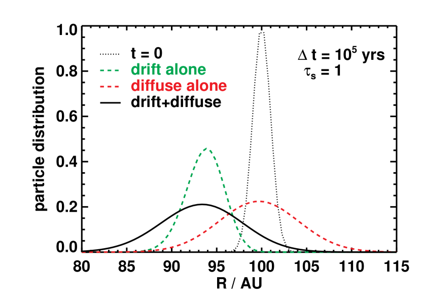
Figure 17: The particle ($\tau_{s}=1$) distribution after $10^{5}$ years due to the effects of radial drift and diffusion (using $D_{\rm{p,x}}=0.1c_{\rm{s}}^{2}/\Omega$). An 1D advection-diffusion model (Adams & Bloch, 2009) is used to evolve the distribution. About $10\%$ of the initial values can still be found at $R=100$ AU (black solid) in contrast to the radial drift alone case (green dashed) where nearly all particles drift out of $R=100$ AU.

4.2.2 Fragmentation and run-away accretion barriers

Large relative velocity between particle pairs might lead to catastrophic disruptions. For micron-to-meter-sized particles, the critical collisional speeds which would results in fragmentation is $v_{\rm f}\gtrsim 1\,\rm{m}\,\rm{s^{-1}}$ (Blum & Wurm, 2008; Stewart & Leinhardt, 2009; Carballido et al., 2010), which is $\gtrsim 0.01c_{\rm{s}}$ in our disk. Based on the probability distribution function of relative velocity for the equal-sized particles (bottom left panel of Figure 8), particles of decimeter or smaller ($\tau_{s}\leq 1$) are mostly below this fragmentation barrier.

As particle grows even bigger, its self-gravity would strengthen the particle against catastrophic disruption. The criteria of fragmentation is such that the specific kinetic energy of a collision ($v_{\rm rel}^{2}/2$) exceeds the critical disruption energy

$$Q_{\rm D}\simeq\left[Q_{0}\left(\frac{s}{1\rm{cm}}\right)^{a}\!\!+B\left(\frac{\rho_{s}}{1\rm{g}\,\rm{cm^{-3}}}\right)\left(\frac{s}{1\rm{cm}}\right)^{b}\right]\,\rm{erg}\,\rm{g^{-1}}\,,$$ (21)

where $Q_{0}\sim 10^{7}\rm{-}10^{8}$ is the material strength, $B\simeq 0.3\rm{-}2.1$ parameterize the self-gravity effect, $a\simeq-0.4$, and $b\simeq 1.3$ for pair-collisions between equal-sized particles (Benz & Asphaug, 1999; Ida et al., 2008). We note that different material properties, projectile-to-target mass ratio and impact velocity could all cause differences in this criteria (Stewart & Leinhardt, 2009). Therefore, we should take the above energy criteria as a rough order-of-magnitude estimation.

Following Ida et al. (2008) and using Equation 21, we find that a collision results in destruction if the relative velocity exceeds the fragmentation velocity

$$v_{\rm f}\simeq 0.13c_{\rm{s}}\left(\frac{s}{1\,\rm{km}}\right)^{0.65}\left(\frac{\rho_{s}}{3\,\rm{g}\,\rm{cm^{-3}}}\right)^{1/2}\left(\frac{R}{100\,\rm{AU}}\right)^{1/2}\,.$$ (22)

Thus particles with ${\rm{m}}\leq s\leq{\rm{km}}$ ($10\leq\tau_{s}\leq 10^{4}$) would have fragmentation velocity $\sim(0.01{\rm{-}}0.1)c_{\rm{s}}$, much lower than the most probable relative velocity of those particles found in our simulations (see again the bottom left panel of Figure 8). The high relative velocity found in our gravito-turbulent disks would therefore limit the size that the majority of planetesimal formation could reach.

If the main channel of planetesimal formation is through gravitational run-away accretion, it would require the relative velocity to be even lower than the escape velocity of the collisional outcome (Ida et al., 2008; Okuzumi & Ormel, 2013; Ormel & Okuzumi, 2013),

$$v_{\rm esc}\simeq 4\times 10^{-3}c_{\rm{s}}\left(\frac{s}{1\,\rm{km}}\right)\left(\frac{\rho_{s}}{3\,\rm{g}\,\rm{cm^{-3}}}\right)^{1/2}\left(\frac{R}{100\,\rm{AU}}\right)\,.$$ (23)

The planetesimal formation from collisional accretion is strongly disfavored in our gravito-turbulent disks.

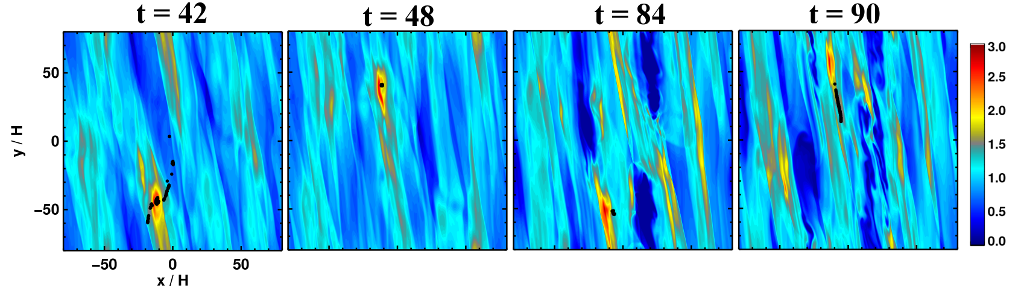
Figure 18: Illustration of the time evolution of the dust concentration for $\Omega t_{\rm{cool}}=40$ run, in which a selection of particles ($\sim 20,000$ in number) with $\tau_{s}=1$ are marked as black dots, and the color contour at the background shows the density fluctuation in linear scale. We first identify a high density ($\Sigma_{p}\gtrsim 1000$) particle cluster at $t=48\Omega^{-1}$, as show in the second panel with black dots. We then track each individual particles backward/forward in time. The compact cluster disappears only after $t=84\Omega^{-1}$, which lasts nearly $6$ orbits before being sheared away.

There are a few conditions that might allay the difficulties: (1) When taking into account of $t_{\rm{cool}}$, a longer cooling time scale would reduce the relative velocity (only weakly depends on $t_{\rm{cool}}$ though; see Figure 14) and thus lower the possibility of fragmentation. (2) We note the distribution functions show a sizeable spread toward smaller relative velocity, therefor a small fraction of planetesimals might still survive the collision or even accrete although the mean relative velocity is high (Windmark et al., 2012). (3) The strong diffusion may bring planetesimals outside the gravito-turbulent zone, and proceed further growth in a less violent environment. (4) If the pre-existing sizes of the planetesimals are big enough, they might avoid fragmentation and/or run-away barrier since $v_{\rm rel}$ scales with $\tau_{s}$ differently than $v_{\rm esc}$ and $v_{\rm f}$ do. We find $v_{\rm rel}/c_{\rm{s}}\simeq(\tau_{s}/10)^{0.16}$ after extrapolating our relative speed results in the bottom left panel of Figure 14 toward high $\tau_{s}$ end. We thus find only planetesimals $\gtrsim 100\,{\rm km}$ could pass the fragmentation barrier; only $\gtrsim 1000\,{\rm km}$-sized planetesimals would result in collisional accretion. Such large planetesimals might form via gravitational instability as we will discuss next.

4.2.3 Gravitational collapse

Despite the problems caused by the big relative velocity for particles bigger than meter-size, those cm-to-decimeter-sized ($\tau_{s}=0.1\rm{-}1$) pebbles, find themselves mostly in very dense coherent structures and possessing very low relative velocities. As shown in Figure 2 and 15, the concentration factor $\Sigma_{\rm p}/\langle\Sigma_{\rm p}\rangle$ is typically $\gtrsim 10$-$100$ in those filament-like structures. Concentrations can go even higher than $\gtrsim 100$-$10^{3}$ times the original particle density for longer cooling time $t_{\rm{cool}}=40\Omega^{-1}$. This density enhancement of the dust particles would push the dust-to-gas ratio from $\sim 1/100$ to $\Sigma_{\rm p}/\Sigma_{g}\gtrsim 10$. More importantly, the resulting local dust density

$$\rho_{\rm p}\gtrsim 10^{-12}\left(\frac{\Sigma_{\rm p}/\Sigma_{g}}{10}\right){\rm g}\,{\rm cm^{-3}}\,,$$ (24)

will exceed the Roche density

$$\rho_{\rm Roche}\sim\frac{M_{*}}{R^{3}}\sim 10^{-12}\left(\frac{M_{*}}{M_{\odot}}\right)\left(\frac{R}{100\,\rm{AU}}\right)^{-3}\,,$$ (25)

where $M_{*}$ is the stellar mass, and therefore trigger gravitational collapse. This opens up a potential channel of planetesimal formation via gravitational collapse (Boss, 2000; Britsch et al., 2008; Gibbons et al., 2012, 2014; Shi & Chiang, 2013). In Figure 18, we show a clump of $\tau_{s}=1$ particles which possess over-density $\Sigma_{\rm p}/\langle\Sigma_{\rm p}\rangle\gtrsim 10^{3}$ could survive for $\simeq 6\,{\rm orbits}$, or $6,000{\rm yr}$ at $R=100\,\rm{AU}$, before getting disrupted in a gravito-turbulent disk with $\Omega t_{\rm{cool}}=40$. This is significantly longer than the dynamical time that is necessary for the process of gravitational collapse. Even if the dust density does not cross the Roche density, the $\rho_{\rm p}\sim\rho_{g}$ in our gravito-turbulent disks could still trigger other instabilities such as streaming instability (Goodman & Pindor, 2000; Youdin & Goodman, 2005) for those intermediate size particles. As a result, the dust density increases further and graviational collapse would still occur eventually. The resulting planetesimals would then diffuse out the gravito-turbulent region as discussed in section 4.2.1 and avoid being destroyed (if $s\lesssim 100\,\rm{km}$) due to collision with planetesimals of the same size.

4.2.4 Comparison with MRI-driven turbulent disks

In general, we find relatively stronger radial diffusion and eccentricity growth in our gravito-turbulent disks than in MRI-driven turbulent disks of similar $\alpha$.

According to Yang et al. (2009, 2012), the standard deviation of radial drift can be described as

$$\sigma(\Delta x)=C_{x}\,\xi\,H\left(\frac{t\Omega}{2\pi}\right)^{1/2}\,,$$ (26)

where $C_{x}$ is a dimensionless coefficient and $\xi\equiv 4\pi G\rho_{0}(2\pi/\Omega)^{2}=4(2\pi)^{3/2}/Q$ assuming $\rho_{0}=\Sigma_{0}/2H$. Comparing it with Equation (10), we can convert our diffusion coefficient to

$$C_{x}\simeq 0.056\,Q\left(\frac{D_{\rm{p,x}}}{c_{\rm{s}}^{2}/\Omega}\right)^{1/2}\,.$$ (27)

Take our standard tc=10 run ($\alpha\simeq 0.02$) as an example, $D_{\rm{p,x}}\geq 0.05c_{\rm{s}}^{2}/\Omega$ for large particles with $\tau_{s}>1$, we therefore obtain a dimensionless $C_{x}\geq 0.038$, more than one order of magnitude larger than $C_{x}$ measured in MRI disks (cf. Table 1 in Nelson & Gressel (2010) and Table 2 in Yang et al. (2012)).

The excitation of eccentricity can also be described as (Yang et al., 2009, 2012)

$$\sigma(\Delta e)=C_{e}\,\xi\left(\frac{H}{R}\right)\left(\frac{t\Omega}{2\pi}\right)^{1/2}\,,$$ (28)

where $C_{e}$ is a dimensionless coefficient characterizes the growth rate. After comparing it with Equation 14, we have

$$C_{e}\simeq 0.040\,QC\,.$$ (29)

Recalling $C\simeq 0.15$ for $\tau_{s}=10^{2}$ when $\Omega t_{\rm{cool}}=10$ in section 3.3, we find the typical $C_{e}\simeq 0.018$, much greater than $10^{-3}$–$10^{-4}$ found in Yang et al. (2012) using local shearing boxes, and one order of magnitude greater than reported in Nelson & Gressel (2010) with global simulations.

The increasing eccentricity and diffusion is a result of stronger gravitational forcing in gravito-turbulent disk than in MRI disk. Quantitatively, the parameter $\gamma$ (closely related to $\delta\Sigma/\Sigma$) reflects the strength of this stirring. As discussed in section 3.7 and also shown in Table 1, this dimensionless parameter $\gamma$ is at least one order of magnitude larger than found in MRI disks (e.g., Yang et al., 2012). As discussed in section 3.5, the stronger forcing also pushes more types of particles ($\tau_{s}>1$) into the gravity dominated regime; while in MRI disk, as shown in Figure 15 and 23 of Nelson & Gressel (2010), this occurs only for particles with $\tau_{s}>100$.

5 SUMMARY AND CONCLUSION

We have studied the dynamics of dust in gravito-turbulent disks, i.e., gaseous disks whose turbulence is driven by self-gravity, using 2D hybrid (particle and gas) simulations in a local shearing sheet approximation. For dust particles, we included the aerodynamic drag and gravitational pull from self-gravitating gas, and neglected particle self-gravity and feedback. We obtained the density distribution, radial diffusion coefficient and relative velocities for dust particles with stopping times distributed from $10^{-3}\Omega^{-1}$ to $10^{3}\Omega^{-1}$. We summarize our main results as follows:

1. Particles with small stopping times ($\tau_{s}<0.1$) are aerodynamically well-coupled to gas and therefore trace the gas distribution. Diffusion coefficients for small particles are close to those for gas. The gas diffusion coefficient $D_{\rm{g,x}}$ is related to the angular momentum transport parameter $\alpha$ via a roughly constant Schmidt number ${\rm Sc}=\alpha/D_{\rm{g,x}}=1.4{\rm-}2.4$. Small particles also have low eccentricities ($e\sim 0.1(H/R)(\alpha/0.01)^{1/2}$) and low relative velocities ($\lesssim 0.01{\rm-}0.1\,(\alpha/0.01)^{1/2}c_{\rm{s}}$).

2. Particles with larger stopping times ($\tau_{s}\gtrsim 1$) are more strongly gravitationally forced from self-gravitating gas than by aerodynamic drag. The stronger forcing results in diffusion coefficients that are $\gtrsim 5$ times greater than those of smaller particles. Turbulent diffusion in gravito-turbulent disks therefore plays an important role in radial transport of large bodies. Strong stochastic gravitational stirring generates large eccentricities ($e\gtrsim 0.5{\rm-}1(H/R)(\alpha/0.01)^{1/2}$) and large relative velocity ($\gtrsim(\alpha/0.01)^{1/2}c_{\rm{s}}$). These disfavor planetesimal formation by pairwise collision as the typical collisional speed exceeds both the escape and fragmentation velocities.

3. Particles of intermediate size ($\tau_{s}=0.1{\rm-}1$) are marginally coupled to gas, and are collected by both gas drag and gravitational torques (see equation 17) into filament-like structures having large overdensities ($\gtrsim 10{\rm-}10^{3}$ times the background) and low relative velocities ($\lesssim 0.01c_{\rm{s}}$) between like-sized particles. The density concentration is high enough to trigger direct gravitational collapse. Nascent planetesimals can avoid collisional disruption by diffusing to less turbulent regions of the disk.

4. Longer cooling times result in weaker turbulence ($\alpha\propto(\Omega t_{\rm{cool}})^{-1}$), weaker particle diffusion ($\propto\alpha$), lower relative velocities and eccentricities ($\propto\sqrt{\alpha}$), and stronger clustering for intermediate-size ($\tau_{s}=0.1{\rm-}1$) particles.

5. Compared to MRI-turbulent disks, gravito-turbulent disks show almost one order-of-magnitude stronger density fluctuations for similar $\alpha$ ($\delta\Sigma/\Sigma\simeq 5\sqrt{\alpha}$ versus $\sqrt{0.5\alpha}$). Stronger gravitational stirring leads to higher eccentricities and relative velocities between particles.

In a recent paper that parallels ours, Booth & Clarke (2016) study the relative velocities of dust particles in global smoothed-particle hydrodynamics (SPH) simulations of gravito-turbulent protoplanetary disks. Like us, they find large relative velocities for particles with $\tau_{s}\gtrsim 3$ (compare our Figure 8 with their Figures 6 and 7).

Future investigations could improve upon our work in any number of ways. As we use massless test particles in 2D hydrodynamic local simulations with a simplistic cooling prescription, the effects of vertical sedimentation, particle feedback, particle self-gravity (Gibbons et al., 2014), and self-consistent heating and cooling on dust dynamics could be further explored. Local and eventually global 3D simulations which account for these physical effects would be clear next steps.

References

- Adams & Bloch (2009) Adams F. C., Bloch A. M., 2009, ApJ, 701, 1381
- Alexander et al. (2008) Alexander C. M. O. ., Grossman J. N., Ebel D. S., Ciesla F. J., 2008, Science, 320, 1617
- Andrews (2015) Andrews S. M., 2015, PASP, 127, 961
- Andrews & Williams (2007) Andrews S. M., Williams J. P., 2007, ApJ, 671, 1800
- Armitage (2011) Armitage P. J., 2011, ARA&A, 49, 195
- Bai & Stone (2010) Bai X.-N., Stone J. M., 2010, ApJS, 190, 297
- Balbus & Hawley (1991) Balbus S. A., Hawley J. F., 1991, ApJ, 376, 214
- Balbus & Hawley (1998) Balbus S. A., Hawley J. F., 1998, Reviews of Modern Physics, 70, 1
- Barranco & Marcus (2005) Barranco J. A., Marcus P. S., 2005, ApJ, 623, 1157
- Benz & Asphaug (1999) Benz W., Asphaug E., 1999, Icarus, 142, 5
- Blum & Wurm (2008) Blum J., Wurm G., 2008, ARA&A, 46, 21
- Booth & Clarke (2016) Booth R. A., Clarke C. J., 2016, preprint, (arXiv:1603.00029)
- Boss (2000) Boss A. P., 2000, ApJ, 536, L101
- Boss (2015) Boss A. P., 2015, ApJ, 807, 10
- Britsch et al. (2008) Britsch M., Clarke C. J., Lodato G., 2008, MNRAS, 385, 1067
- Carballido et al. (2010) Carballido A., Cuzzi J. N., Hogan R. C., 2010, MNRAS, 405, 2339
- Carballido et al. (2011) Carballido A., Bai X.-N., Cuzzi J. N., 2011, MNRAS, 415, 93
- Cheng (2009) Cheng N.-S., 2009, Powder Technology, 189, 395
- Chiang & Youdin (2010) Chiang E., Youdin A., 2010, Annual Reviews of Earth and Planetary Science, 38
- Cossins et al. (2009) Cossins P., Lodato G., Clarke C. J., 2009, MNRAS, 393, 1157
- Cuzzi & Alexander (2006) Cuzzi J. N., Alexander C. M. O., 2006, Nature, 441, 483
- Cuzzi et al. (1993) Cuzzi J. N., Dobrovolskis A. R., Champney J. M., 1993, Icarus, 106, 102
- Eisner et al. (2005) Eisner J. A., Hillenbrand L. A., Carpenter J. M., Wolf S., 2005, ApJ, 635, 396
- Flaherty et al. (2015) Flaherty K. M., Hughes A. M., Rosenfeld K. A., Andrews S. M., Chiang E., Simon J. B., Kerzner S., Wilner D. J., 2015, ApJ, 813, 99
- Forgan et al. (2012) Forgan D., Armitage P. J., Simon J. B., 2012, MNRAS, 426, 2419
- Gammie (2001) Gammie C. F., 2001, ApJ, 553, 174
- Garaud et al. (2013) Garaud P., Meru F., Galvagni M., Olczak C., 2013, ApJ, 764, 146
- Gibbons et al. (2012) Gibbons P. G., Rice W. K. M., Mamatsashvili G. R., 2012, MNRAS, 426, 1444
- Gibbons et al. (2014) Gibbons P. G., Mamatsashvili G. R., Rice W. K. M., 2014, MNRAS, 442, 361
- Gibbons et al. (2015) Gibbons P. G., Mamatsashvili G. R., Rice W. K. M., 2015, MNRAS, 453, 4232
- Goldreich & Lynden-Bell (1965) Goldreich P., Lynden-Bell D., 1965, MNRAS, 130, 125
- Goodman & Pindor (2000) Goodman J., Pindor B., 2000, Icarus, 148, 537
- Gressel et al. (2012) Gressel O., Nelson R. P., Turner N. J., 2012, MNRAS, 422, 1140
- Guyer et al. (2009) Guyer J. E., Wheeler D., Warren J. A., 2009, Computing in Science & Engineering, 11, 6
- Ida et al. (2008) Ida S., Guillot T., Morbidelli A., 2008, ApJ, 686, 1292
- Jacquet & Thompson (2014) Jacquet E., Thompson C., 2014, ApJ, 797, 30
- Johansen et al. (2009) Johansen A., Youdin A., Klahr H., 2009, ApJ, 697, 1269
- Johansen et al. (2011) Johansen A., Klahr H., Henning T., 2011, A&A, 529, A62
- Johansen et al. (2014) Johansen A., Blum J., Tanaka H., Ormel C., Bizzarro M., Rickman H., 2014, Protostars and Planets VI, pp 547–570
- Johnson & Gammie (2003) Johnson B. M., Gammie C. F., 2003, ApJ, 597, 131
- Johnson et al. (2006) Johnson E. T., Goodman J., Menou K., 2006, ApJ, 647, 1413
- Johnson et al. (2008) Johnson B. M., Guan X., Gammie C. F., 2008, ApJS, 177, 373
- Klahr & Bodenheimer (2003) Klahr H. H., Bodenheimer P., 2003, ApJ, 582, 869
- Laughlin et al. (2004) Laughlin G., Steinacker A., Adams F. C., 2004, ApJ, 608, 489
- Lodato & Rice (2004) Lodato G., Rice W. K. M., 2004, MNRAS, 351, 630
- Lodato & Rice (2005) Lodato G., Rice W. K. M., 2005, MNRAS, 358, 1489
- Mamatsashvili & Rice (2009) Mamatsashvili G. R., Rice W. K. M., 2009, MNRAS, 394, 2153
- Masset (2000) Masset F., 2000, A&AS, 141, 165
- Maxey (1987) Maxey M. R., 1987, J. Fluid Mech., 174, 441
- Mejía et al. (2005) Mejía A. C., Durisen R. H., Pickett M. K., Cai K., 2005, ApJ, 619, 1098
- Meru & Bate (2011) Meru F., Bate M. R., 2011, MNRAS, 411, L1
- Mitra et al. (2013) Mitra D., Wettlaufer J. S., Brandenburg A., 2013, ApJ, 773, 120
- Nakamoto & Miura (2004) Nakamoto T., Miura H., 2004, in Mackwell S., Stansbery E., eds, Lunar and Planetary Science Conference Vol. 35, Lunar and Planetary Science Conference.
- Nelson (2005) Nelson R. P., 2005, A&A, 443, 1067
- Nelson & Gressel (2010) Nelson R. P., Gressel O., 2010, MNRAS, 409, 639
- Ogihara et al. (2007) Ogihara M., Ida S., Morbidelli A., 2007, Icarus, 188, 522
- Okuzumi & Hirose (2011) Okuzumi S., Hirose S., 2011, ApJ, 742, 65
- Okuzumi & Ormel (2013) Okuzumi S., Ormel C. W., 2013, ApJ, 771, 43
- Ormel & Cuzzi (2007) Ormel C. W., Cuzzi J. N., 2007, A&A, 466, 413
- Ormel & Okuzumi (2013) Ormel C. W., Okuzumi S., 2013, ApJ, 771, 44
- Paardekooper (2012) Paardekooper S.-J., 2012, MNRAS, 421, 3286
- Paczynski (1978) Paczynski B., 1978, Acta Astron., 28, 91
- Pan et al. (2011) Pan L., Padoan P., Scalo J., Kritsuk A. G., Norman M. L., 2011, ApJ, 740, 6
- Pan et al. (2014) Pan L., Padoan P., Scalo J., 2014, ApJ, 792, 69
- Perets & Murray-Clay (2011) Perets H. B., Murray-Clay R. A., 2011, ApJ, 733, 56
- Ricci et al. (2010) Ricci L., Testi L., Natta A., Neri R., Cabrit S., Herczeg G. J., 2010, A&A, 512, A15
- Rice et al. (2003) Rice W. K. M., Armitage P. J., Bate M. R., Bonnell I. A., 2003, MNRAS, 339, 1025
- Rice et al. (2004) Rice W. K. M., Lodato G., Pringle J. E., Armitage P. J., Bonnell I. A., 2004, MNRAS, 355, 543
- Rice et al. (2006) Rice W. K. M., Lodato G., Pringle J. E., Armitage P. J., Bonnell I. A., 2006, MNRAS, 372, L9
- Rodríguez et al. (2005) Rodríguez L. F., Loinard L., D’Alessio P., Wilner D. J., Ho P. T. P., 2005, ApJ, 621, L133
- Shi & Chiang (2013) Shi J.-M., Chiang E., 2013, ApJ, 764, 20
- Shi & Chiang (2014) Shi J.-M., Chiang E., 2014, ApJ, 789, 34
- Shi et al. (2016) Shi J.-M., Stone J. M., Huang C. X., 2016, MNRAS, 456, 2273
- Stewart & Leinhardt (2009) Stewart S. T., Leinhardt Z. M., 2009, ApJ, 691, L133
- Stone & Gardiner (2009) Stone J. M., Gardiner T., 2009, New Astron., 14, 139
- Stone & Gardiner (2010) Stone J. M., Gardiner T. A., 2010, ApJS, 189, 142
- Stone et al. (2008) Stone J. M., Gardiner T. A., Teuben P., Hawley J. F., Simon J. B., 2008, ApJS, 178, 137
- Testi et al. (2014) Testi L., et al., 2014, Protostars and Planets VI, pp 339–361
- Tobin et al. (2013) Tobin J. J., Hartmann L., Chiang H.-F., Wilner D. J., Looney L. W., Loinard L., Calvet N., D’Alessio P., 2013, ApJ, 771, 48
- Toomre (1964) Toomre A., 1964, ApJ, 139, 1217
- Voelk et al. (1980) Voelk H. J., Jones F. C., Morfill G. E., Roeser S., 1980, A&A, 85, 316
- Walmswell et al. (2013) Walmswell J., Clarke C., Cossins P., 2013, MNRAS, 431, 1903
- Weidenschilling (1977) Weidenschilling S. J., 1977, MNRAS, 180, 57
- Weidenschilling & Cuzzi (1993) Weidenschilling S. J., Cuzzi J. N., 1993, in E. H. Levy & J. I. Lunine ed., Protostars and Planets III. pp 1031–1060
- Williams & Cieza (2011) Williams J. P., Cieza L. A., 2011, ARA&A, 49, 67
- Windmark et al. (2012) Windmark F., Birnstiel T., Ormel C. W., Dullemond C. P., 2012, A&A, 544, L16
- Yang et al. (2009) Yang C.-C., Mac Low M.-M., Menou K., 2009, ApJ, 707, 1233
- Yang et al. (2012) Yang C.-C., Mac Low M.-M., Menou K., 2012, ApJ, 748, 79
- Youdin & Goodman (2005) Youdin A. N., Goodman J., 2005, ApJ, 620, 459
- Youdin & Lithwick (2007) Youdin A. N., Lithwick Y., 2007, Icarus, 192, 588
- Zhu et al. (2015) Zhu Z., Stone J. M., Bai X.-N., 2015, ApJ, 801, 81
- van Leer (2006) van Leer B., 2006, Comm. Comput. Phys., 1, 192