Classification of joint numerical ranges of three hermitian matrices of size three

Abstract.

The joint numerical range $W(F)$ of three hermitian $3$-by-$3$ matrices $F=(F_{1},F_{2},F_{3})$ is a convex and compact subset in $\mathbb{R}^{3}$. We show that $W(F)$ is generically a three-dimensional oval. Assuming $\dim(W(F))=3$, every one- or two-dimensional face of $W(F)$ is a segment or a filled ellipse. We prove that only ten configurations of these segments and ellipses are possible. We identify a triple $F$ for each class and illustrate $W(F)$ using random matrices and dual varieties.

Classification of joint numerical ranges

1. Introduction

We denote the space of complex $d$-by-$d$ matrices by $M_{d}$, the real subspace of hermitian matrices by $M^{\rm h}_{d}:=\{a\in M_{d}\mid a^{*}=a\}$, and the identity matrix by $\mathds{1}_{d}\in M_{d}$. We write $\langle x,y\rangle:=\overline{x_{1}}y_{1}+\cdots+\overline{x_{d}}y_{d}$, $x,y\in\mathbb{C}^{d}$ for the inner product on $\mathbb{C}^{d}$. For $d,n\in\mathbb{N}=\{1,2,3,\ldots\}$, let $F:=(F_{1},\ldots,F_{n})\in(M^{\rm h}_{d})^{n}$ be an $n$-tuple of hermitian $d$-by-$d$ matrices. The joint numerical range of $F$ is

$$W(F):=\{(\langle x,F_{1}x\rangle,\ldots,\langle x,F_{n}x\rangle)\mid x\in\mathbb{C}^{d},\langle x,x\rangle=1\}\subset\mathbb{R}^{n}.$$

For $n=2$, identifying $\mathbb{R}^{2}\cong\mathbb{C}$, the set $W(F_{1},F_{2})$ is the numerical range $\{\langle x,Ax\rangle\mid x\in\mathbb{C}^{d},\langle x,x\rangle=1\}$ of $A:=F_{1}+\operatorname{i}F_{2}$. The numerical range is convex for all $d\in\mathbb{N}$ by the Toeplitz-Hausdorff theorem [55, 29]. Similarly, for $n=3$ and all $d\geq 3$ the joint numerical range $W(F_{1},F_{2},F_{3})$ is convex [2]. However, $W(F)$ is in general not convex for $n\geq 4$, see [45, 41, 26].

Let $d,n\in\mathbb{N}$ be arbitrary and call $F\in(M^{\rm h}_{d})^{n}$ unitarily reducible if there is a unitary $U\in M_{d}$ such that the matrices $U^{*}F_{1}U,\ldots,U^{*}F_{n}U$ have a common block diagonal form with two proper blocks. Otherwise $F$ is unitarily irreducible.

The shape of the numerical range ($n=2$) is well understood. The elliptical range theorem [40] states that the numerical range of a $2$-by-$2$ matrix is a singleton, segment, or filled ellipse. Kippenhahn [36] proved for all $d\in\mathbb{N}$ and $F\in(M^{\rm h}_{d})^{2}$ that $W(F)$ is the convex hull of the boundary generating curve defined in Remark 1.3. He showed for $3$-by-$3$ matrices ($d=3$) that if $F$ is unitarily reducible, then $W(F)$ is a singleton, segment, triangle, ellipse, or the convex hull of an ellipse and a point outside the ellipse. If $F$ is unitarily irreducible, then $W(F)$ is an ellipse, the convex hull of a quartic curve (with a flat portion on the boundary), or the convex hull of a sextic curve (an oval). Kippenhahn’s result for $3$-by-$3$ matrices was expressed in terms of matrix invariants and matrix entries of $F_{1}+\operatorname{i}F_{2}$, see [35, 49, 47, 54]. The boundary generating curve was also used [16] to find a classification of the numerical range of a $4$-by-$4$ matrix. Another result [31, 30] is that a subset $W$ of $\mathbb{C}$ is the numerical range of some $d$-by-$d$ matrix if and only if it is a translation of the polar of a rigidly convex set of degree less than or equal to $d$, see Corollary 3 of [30]. We omit the details of this last description as we will not use it.

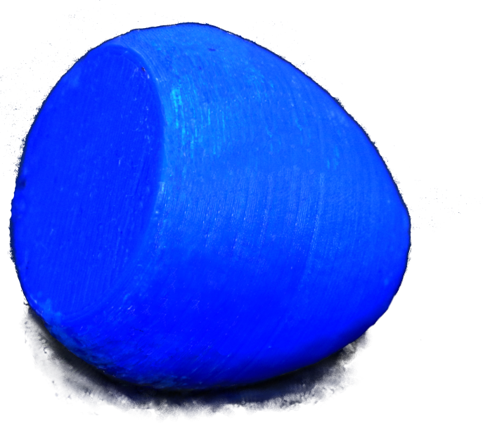
a) Ex. 6.2, $s=0,e=1$

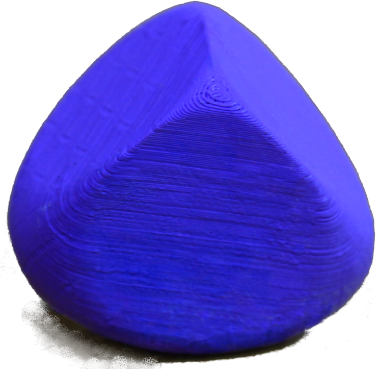
b) Ex. 6.4, $s=0,e=3$

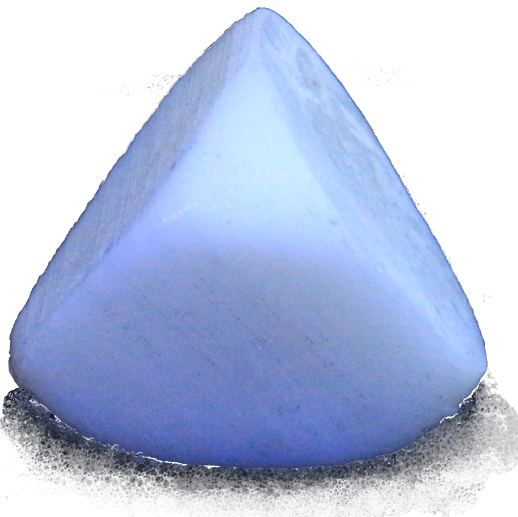
c) Ex. 6.5, $s=0,e=4$

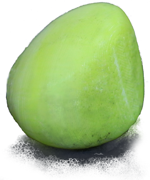
d) Ex. 6.6, $s=1,e=0$

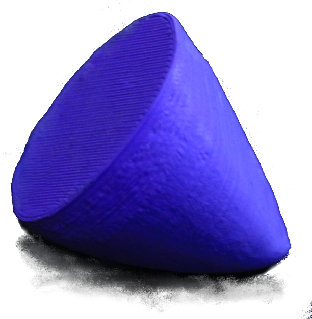
e) Ex. 6.7, $s=1,e=1$

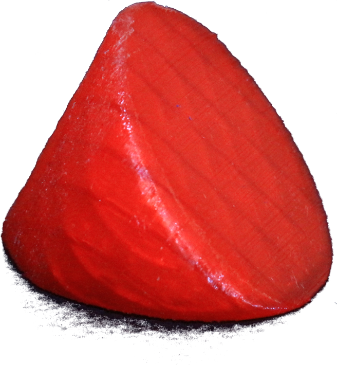
f) Ex. 6.8, $s=1,e=2$

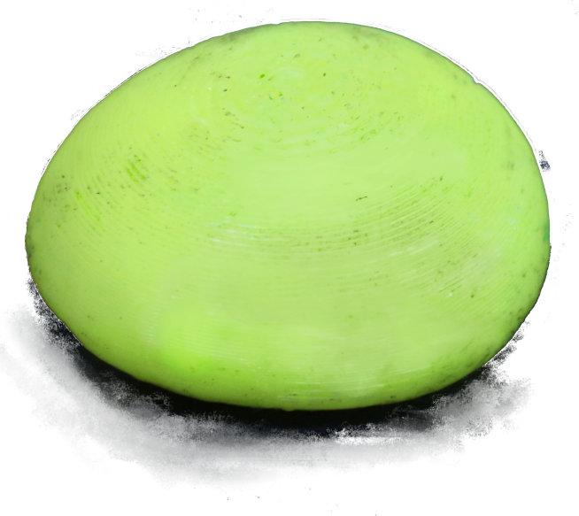
g) $s=e=0$

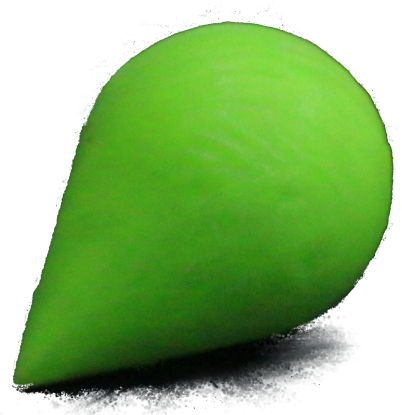
h) $s=\infty,e=0$

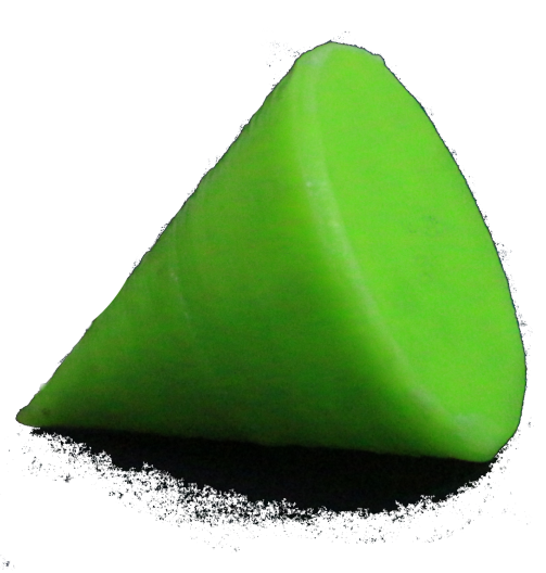
i) $s=\infty,e=1$

Figure 1. 3D printouts of exemplary joint numerical ranges of triples of hermitian 3-by-3 matrices from random density matrices: $s$ denotes the number of segments, $e$ the number of ellipses in the boundary.

Despite the long history of the problem [8, 37, 14, 15, 12], a classification of the joint numerical range of triples of matrices ($n=3$) is unknown even in the case $d=n=3$. Our motivation to tackle this problem is quantum mechanics, as we explain in Section 2. The link to physics is that for arbitrary $d,n\in\mathbb{N}$ and $F\in(M^{\rm h}_{d})^{n}$ the convex hull

$$L(F):=\operatorname{conv}(W(F))$$

of $W(F)$ is a projection (image under a linear map) of the state space $\mathcal{M}_{d}$ of the algebra $M_{d}$ [19]. The state space consists of $d$-by-$d$ density matrices, that is positive semi-definite matrices of trace one, which represent the states of a quantum system.

Until further notice let $d=n=3$, where $L(F)=W(F)$ holds. One of us used random matrices to compute exemplary joint numerical ranges [59]. Photos of their printouts on a 3D-printer are depicted in Figure 1. The printout shown in Figure 1f) was the starting point of this research. As a result we present a simple classification of $W(F)$ in terms of exposed faces. An exposed face of $W(F)$ is a subset of $W(F)$ which is either empty or consists of the maximizers of a linear functional on $W(F)$. Lemma 4.3 shows that the non-empty exposed faces of $W(F)$ which are neither singletons nor equal to $W(F)$ are segments or filled ellipses. We call them large faces of $W(F)$ and collect them in the set

(1.1) $$\mathcal{L}(F)\,:=\,\{ \mbox{$G$ is an exposed face of $W(F)$}\mid$$

$$\mbox{$G\neq W(F)$ and $G$ is a segment or a filled ellipse}\}.$$

Let $e$ (resp. $s$) denote the number of filled ellipses (resp. segments) in $\mathcal{L}(F)$. We recall that a corner point of $W(F)$ is a point which lies on three supporting hyperplanes with linearly independent normal vectors.

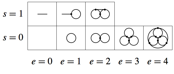
Figure 2. Possible configurations of large faces of a joint numerical range without corner points for $d=n=3$. Circles (resp. segments) denote large faces which are filled ellipses (resp. segments). Dots denote intersection points between large faces.

Theorem 1.1.

Let $F\in(M^{\rm h}_{3})^{3}$. If $W(F)$ has no corner point, then the set $\mathcal{L}(F)$ of large faces of $W(F)$ has one of the eight configurations of Figure 2.

Proof: It is easy to see that large faces intersect mutually (Lemma 5.1). Since $W(F)$ has no corner point, no point lies on three mutually distinct large faces (Lemma 5.2). Hence the union of large faces contains an embedded complete graph with one vertex at the centroid of each large face (Lemma 5.3). Now, a well-known theorem of graph embedding [48] shows $e+s\leq 4$. We observe that $s=0,1$ holds, because for $s\geq 2$ the set $W(F)$ has a corner point (Lemma 5.4). We exclude the case $(e,s)=(3,1)$ by noting that for $s\geq 1$ the embedded complete graph has a vertex on a segment. Then the graph has vertex degree at most two which implies $e+s\leq 3$. $\square$

Section 6 shows three-dimensional examples of $W(F)$ without corner points for all configurations of Figure 2. We are unaware of earlier examples of

$$(e,s)\quad=\quad(1,0),\quad(2,0),\quad(3,0),\quad\mbox{and}\quad(0,1).$$

Ovals, where $(e,s)=(0,0)$, are studied in [37]. An example of $(e,s)=(4,0)$ is in [32], one of $(e,s)=(1,1)$ is in [15], and one of $(e,s)=(2,1)$ is in [9].

If $\dim(W(F))=3$ and $W(F)$ has corner points, then Lemma 4.10 shows that $W(F)$ is the convex hull of an ellipsoid and a point outside the ellipsoid, where $(e,s)=(0,\infty)$, or the convex hull of an ellipse and a point outside the affine hull of the ellipse, where $(e,s)=(1,\infty)$. Examples are depicted in Figure 1h) and 1i).

If $\dim(W(F))=2$ then $e=0$. By projecting to a plane, $W(F)$ corresponds to the numerical range of a 3-by-3 matrix. Notice that $W(F)$ belongs to one of four classes of 2D objects characterized by the number of segments $s=0,1,2,3$. The classification of $W(F)$ in terms of this number $s$ is courser than that explained above [36]. An object with $s=0$ can be an ellipse or the convex hull of a sextic curve.

Remark 1.2 (Limits of extreme points).

Three-dimensional joint numerical ranges of $F\in(M^{\rm h}_{3})^{3}$ solve a problem posed in [57]. A limit of extreme points of $\mathcal{M}_{d}$, $d\in\mathbb{N}$, is again an extreme point and the question is whether the analogue holds for projections of $\mathcal{M}_{d}$. This doubt is dispelled by observing for $(e,s)=(0,1),(1,1),(2,1)$ that any point in the relative interior of the segment in $\mathcal{L}(F)$ is a limit of extreme points of $W(F)$ but no extreme point itself, see Figure 4. The problem was already solved in Example 6 of [9] and discussed in Example 4.2 of [50] with an example of $(e,s)=(2,1)$. A simpler example, with larger matrices, is

$$F_{1}=\left(\begin{smallmatrix}1&0&0&0\\ 0&-1&0&0\\ 0&0&1&0\\ 0&0&0&1\end{smallmatrix}\right),\qquad F_{2}=\left(\begin{smallmatrix}0&1&0&0\\ 1&0&0&0\\ 0&0&0&0\\ 0&0&0&0\end{smallmatrix}\right),\qquad F_{3}=\left(\begin{smallmatrix}0&0&0&0\\ 0&0&0&0\\ 0&0&-1&0\\ 0&0&0&1\end{smallmatrix}\right),$$

where $W(F_{1},F_{2},F_{3})$ is the convex hull of the union of the unit disk in the $x$-$y$-plane with the points $(1,0,\pm 1)$.

Remark 1.3 (Real varieties).

For arbitrary $d,n\in\mathbb{N}$ we consider the hypersurface in the complex projective space $\mathbb{P}^{n}$, defined as the zero locus

$$\textstyle S_{F}:=\{(u_{0}:\cdots:u_{n})\in\mathbb{P}^{n}\mid\det(u_{0}\mathds{1}+u_{1}F_{1}+\cdots+u_{n}F_{n})=0\}.$$

An analysis of singularities of $S_{F}$ for $d=n=3$ shows that $W(F)$ has at most four large faces which are ellipses [14]. This estimate also follows from our classification. The dual variety $S_{F}^{*}\subset\mathbb{P}^{n}{}^{*}$ is the complex projective variety which is the closure of the set of tangent hyperplanes of $S_{F}$ at smooth points [22, 28, 24]. The boundary generating hypersurface [15] of $F$ is the real affine part of the dual variety,

$$S_{F}^{*}(\mathbb{R}):=\{(x_{1},\ldots,x_{n})\in\mathbb{R}^{n}\mid(1:x_{1}:\cdots:x_{n})\in S_{F}^{*}\}.$$

For $n=2$, the variety $S_{F}^{*}(\mathbb{R})$ is called boundary generating curve, and Kippenhahn [36] showed that the convex hull of $S_{F}^{*}(\mathbb{R})$ is the numerical range $W(F_{1},F_{2})$. A more detailed proof is given in [15]. For $d=n=3$, Chien and Nakazato [15] discovered that $S_{F}^{*}(\mathbb{R})$ can contain (unbounded) lines, so the analogue of the Kippenhahn assertion is wrong for $n\geq 3$. We will see examples of such lines in Section 6.

Section 4 studies exposed faces. One result is that the joint numerical range of $F\in(M^{\rm h}_{3})^{3}$ is generically an oval, that is a compact strictly convex set with interior points and smooth boundary. More generally, Theorem 4.2 shows that $L(F)=\operatorname{conv}(W(F))$ is generically an oval for all $d\geq 2$ and $n\leq 3$, using the von Neumann-Wigner non-crossing rule [44, 26] and results about normal cones developed in Section 3. Using the crossing rule [23], Lemma 4.7 shows that $W(F)$ is no oval for $d=3$, $n\geq 6$. Among real matrices, ovals are generic for $d\geq 2$ and $n\leq 2$, but do not appear for $d=3$ and $n\geq 4$. We also point out in Section 4 that the discriminant vanishes at normal vectors of large faces. This gives an easy to check condition for the (non-) existence of large faces, because a sum of squares decompositions of the modulus of the discriminant [33] can be used.

Acknowledgements. SW thanks Didier Henrion, Konrad Schmüdgen, and Rainer Sinn for discussions. It is a pleasure to thank the "Complexity Garage" at the Jagiellonian University, where all the 3D printouts were made, and to Lia Pugliese for taking their photos. We acknowledge support by a Brazilian Capes scholarship (SW), by the Polish National Science Center under the project number DEC-2011/02/A/ST1/00119 (KŻ) and by the project #56033 financed by the Templeton Foundation. Research was partially completed while SW was visiting the Institute for Mathematical Sciences, National University of Singapore in 2016.

2. Quantum states

Our interest in the joint numerical range is its role in quantum mechanics where the hermitian matrices $M^{\rm h}_{d}$ are called Hamiltonians or observables, see e.g. [7], and they correspond to physical systems with $d$ energy levels or measurable quantities having $d$ possible outcomes.

Usually a (complex) C*-subalgebra $\mathcal{A}$ of $M_{d}$ is considered as the algebra of observables of a quantum system [1]. If $a\in M_{d}$ is positive semi-definite then we write $a\succeq 0$. The physical states of the quantum system are described by $d$-by-$d$ density matrices which form the state space of $\mathcal{A}$,

(2.1) $$\mathcal{M}(\mathcal{A}):=\{\rho\in\mathcal{A}\mid\rho\succeq 0,\operatorname{tr}(\rho)=1\}.$$

It is well-known that $\mathcal{M}(\mathcal{A})$ is a compact convex subset of $M^{\rm h}_{d}$, see for example Theorem 4.6 of [1]. We are mainly interested in $\mathcal{M}_{d}:=\mathcal{M}(M_{d})$, but in Sec. 4 also in the compressed algebra $pM_{d}p$ where $p\in M_{d}$ is a projection, that is $p^{2}=p^{*}=p$. The state space $\mathcal{M}(pM_{d}p)$ is, as we recall in Sec. 4, an exposed face of $\mathcal{M}_{d}$, see [1, 56]. The state space $\mathcal{M}_{2}$ is a Euclidean ball, called Bloch ball, but $\mathcal{M}_{d}$ is not a ball [7] for $d\geq 3$. Although several attempts were made to analyze properties of this set [34, 6, 52, 38, 25], its complicated structure requires further studies.

We use the inner product $\langle a,b\rangle:=\operatorname{tr}(a^{*}b)$, $a,b\in M_{d}$. For any state $\rho\in\mathcal{M}_{d}$ and Hamiltonian $a\in M^{\rm h}_{d}$, the real number $\langle\rho,a\rangle$ is the expectation value of possible outcomes of measurements of $a$. The state $\rho$ is a pure state if $\rho$ is a rank-one projection. The pure state which is the projection onto the span of a unit vector $x\in\mathbb{C}^{d}$ is denoted by $\rho=|x\rangle\langle x|$ and

$$\langle\rho,a\rangle=\langle|x\rangle\langle x|,a\rangle=\langle x,ax\rangle.$$

Therefore, the standard numerical range $W(a)$ of a hermitian matrix $a$ is the set of expectation values of $a$ obtained from all pure states. An arbitrary state of $\mathcal{M}_{d}$, which may not be pure, is called a mixed state. The spectral theorem applied to a mixed state shows that the convex hull of $W(a)$ is the set of expectation values of $a$ obtained from all mixed states. Since $W(a)$ is convex, no convex hull operation is needed and therefore $W(a)$ can be identified as a projection of $\mathcal{M}_{d}$ onto a line.

Similarly, the standard numerical range $W(F_{1},F_{2})$ of a non-hermitian operator $F_{1}+\operatorname{i}F_{2}$ is convex. So $W(F_{1},F_{2})$ is the set of the expectation values of measurements of two hermitian operators $F_{1}$ and $F_{2}$ performed on two copies of the same mixed quantum state. In other words, $W(F_{1},F_{2})$ is a projection of $\mathcal{M}_{d}$ onto a two-plane [19, 46]. The Dvoretzky theorem [20] implies that for large dimension $d$ a generic 2D projection of the convex set $\mathcal{M}_{d}$ is close to a circular disk, so that the numerical range of a non-hermitian random matrix of the Ginibre ensemble typically forms a disk [17].

In this work we analyze joint numerical ranges of triples of hermitian matrices of size three. These joint numerical ranges are convex and can be interpreted as sets of expectation values of three hermitian observables performed on three copies of the same mixed quantum state. They form projections of the 8D set of density matrices of size three into a three-plane [27].

An example of projection into high-dimensional planes is the map from the states of a composite system to marginals of subsystems. The geometry of three-dimensional projections of two-party marginals was recently studied [58, 10, 11] to investigate many-body quantum systems.

To formalize the discussion of expectation values and projections of the set $\mathcal{M}_{d}$ we consider arbitrary $d,n\in\mathbb{N}$ and $n$ hermitian matrices $F=(F_{1},\ldots,F_{n})\in(M^{\rm h}_{d})^{n}$ of size $d$. We will use the linear map

$$\textstyle\mathbb{E}_{F}:M^{\rm h}_{d}\to\mathbb{R}^{n},\quad a\mapsto(\langle a,F_{1}\rangle,\ldots,\langle a,F_{n}\rangle)$$

to study the image

(2.2) $$\textstyle L(F):=\mathbb{E}_{F}(\mathcal{M}_{d})=\{\mathbb{E}_{F}(\rho)\mid\rho\in\mathcal{M}_{d}\}\subset\mathbb{R}^{n}$$

of the state space $\mathcal{M}_{d}=\mathcal{M}(M_{d})$ defined in (2.1). The set $L(F)$ was called joint algebraic numerical range [43], also convex support [56] in analogy with statistics [4]. The compact convex set $L(F)$ is the convex hull of the joint numerical range

(2.3) $$\textstyle L(F)=\operatorname{conv}(W(F)).$$

Proofs of equation (2.3) can be found in [43, 27]. We recall that $L(F)=W(F)$ holds for $n=3$ and $d\geq 3$ where $W(F)$ is convex. In what follows, we will work mostly with $L(F)$ rather than $W(F)$.

Some of the 3D images shown in Figure 1 are generated using random sampling – this method is simple conceptually and produces objects which are accurate enough for use in printing. In this numerical procedure, which we implemented in Mathematica, we calculate a finite number (of order of $10^{5}$) of points inside $W(F)$,

$$\{(\langle x,F_{1}x\rangle,\ldots,\langle x,F_{n}x\rangle)\mid x\in S\},$$

where $S$ is the set of points sampled from the uniform distribution on the unit sphere of $\mathbb{C}^{d}$ (this step is realized by sampling points from complex $d$-dimensional Gaussian distribution and normalizing the result). A convex hull of generated points is then calculated using ConvexHullMesh procedure and exported to an .stl file, which contains a description of the 3D object recognized by the software used in printing. The final objects were made with PIRX One 3D printer.

3. Normal cones and ovals

We show that joint algebraic numerical ranges have in a sense many normal cones. We prove that this property allows to characterize ovals in terms of strict convexity.

A face of a convex subset $C\subset\mathbb{R}^{m}$, $m\in\mathbb{N}$, is a convex subset of $C$ which contains the endpoints of every open segment in $C$ which it intersects. An exposed face of $C$ is defined as the set of maximizers of a linear functional on $C$. If $C$ is non-empty and compact, then for every $u\in\mathbb{R}^{m}$ the set

(3.1) $$\mathbb{F}_{C}(u):=\operatorname*{argmax}_{x\in C}\langle x,u\rangle$$

is an exposed face of $C$. By definition, the empty set is also an exposed face (then the set of exposed faces forms a lattice). It is well-known that every exposed face is a face. If a face (resp. exposed face) is singleton, then we call its element an extreme point (resp. exposed point). A face (resp. exposed face) of $C$ which is different from $\emptyset,C$ is called proper face (resp. proper exposed face).

Let $C\subset\mathbb{R}^{m}$ be a convex subset and $x\in C$. The normal cone of $C$ at $x$ is

$$N(x):=\{u\in\mathbb{R}^{m}\mid\forall y\in C:\,\langle u,y-x\rangle\leq 0\}.$$

Elements of $N(x)$ are called (outer) normal vectors of $C$ at $x$. It is well-known that there is a non-zero normal vector of $C$ at $x$ if and only if $x$ is a boundary point of $C$. In that case $x$ is smooth if $C$ admits a unique outer unit normal vector at $x$.

The normal cone of $C$ at a non-empty face $G$ of $C$ is well-defined as the normal cone $N(G):=N(x)$ of $C$ at any point $x$ in the relative interior of $G$ (the relative interior of $G$ is the interior of $G$ with respect to the topology of the affine hull of $G$). See for example Section 4 of [57] about the consistency of this definition, and set $N(\emptyset):=\mathbb{R}^{m}$. The convex set $C$ is a convex cone if $C\neq\emptyset$ and if $x\in C$, $\lambda\geq 0$ implies $\lambda x\in C$. A ray is a set of the form $\{\lambda\cdot u\mid\lambda\geq 0\}\subset\mathbb{R}^{m}$ for non-zero $u\in\mathbb{R}^{m}$. An extreme ray of $C$ is a ray which is a face of $C$.

We denote the set of exposed faces and normal cones of $C$ by $\mathcal{E}_{C}$ and $\mathcal{N}_{C}$, respectively. Each of these sets is partially ordered by inclusion and forms a lattice, that is the infimum and supremum of each pair of elements exist. A chain in a lattice is a totally ordered subset, the length of a chain is the cardinality minus one. The length of a lattice is the supremum of the lengths of all its chains. Lattices of faces have been studied earlier [3, 42], in particular these of state spaces [1], and linear images $L(F)$ of state spaces [56]. By Proposition 4.7 of [57], if $C$ is not a singleton then

(3.2) $$\mathcal{E}_{C}\to\mathcal{N}_{C},\quad G\mapsto N(G)$$

is an antitone lattice isomorphism. This means that the map is a bijection and for all exposed faces $G,H$ we have $G\subset H$ if and only if $N(G)\supset N(H)$.

What makes a joint algebraic numerical range $C$ special is that all non-empty faces of its normal cones are normal cones of $C$, too, as we will see in Lemma 3.1. For two-dimensional $C\subset\mathbb{R}^{2}$ this means that a boundary point of $C$ is smooth unless it is the intersection of two one-dimensional faces of $C$, as one can see from the isomorphism (3.2). That property is well-known [5] for the numerical range $W(F_{1},F_{2})$ of a matrix $A=F_{1}+\operatorname{i}F_{2}\in M_{d}$. For example, the half-moon $\{z\in\mathbb{C}:|z|\leq 1,\Re(z)\geq 0\}$ is not the numerical range of any matrix. This also follows from Anderson’s theorem [13] which asserts that if $W(F_{1},F_{2})$ is included in the unit disk and contains $d+1$ distinct points of the unit circle, then $W(F_{1},F_{2})$ is the unit disk.

To prove the lemma we introduce the Definitions 6.1 and 7.1 of [57] for the special case of a non-empty, compact, and convex subset $C\subset\mathbb{R}^{m}$. Let $u\in\mathbb{R}^{m}$ be a non-zero vector. Then $u$ is called sharp normal for $C$ if for every relative interior point $x$ of the exposed face $\mathbb{F}_{C}(u)$ the vector $u$ is a relative interior point of the normal cone of $C$ at $x$. The touching cone of $C$ at $u$ is defined to be the face of the normal cone of $C$ at $\mathbb{F}_{C}(u)$ which contains $u$ in its relative interior [53]. The linear space $\mathbb{R}^{m}$ and the orthogonal complement of the translation vector space of the affine hull of $C$ are touching cones of $C$ by definition. We point out that every normal cone of $C$ is a touching cone of $C$.

Lemma 3.1.

Every non-empty face of every normal cone of $L(F)$ is a normal cone of $L(F)$.

Proof: Propositions 2.9 and 2.11 of [56] prove that every non-zero hermitian $d$-by-$d$ matrix is sharp normal for the state space $\mathcal{M}_{d}$. Therefore, Proposition 7.6 of [57] shows that every touching cone of $\mathcal{M}_{d}$ is a normal cone of $\mathcal{M}_{d}$. Corollary 7.7 of [57] proves that $L(F)$, being a projection of $\mathcal{M}_{d}$, has the analogous property that every touching cone of $L(F)$ is a normal cone of $L(F)$. The characterization of touching cones as the non-empty faces of normal cones, given in Theorem 7.4 of [57], completes the proof. $\square$

We define an oval as a convex and compact subset of $\mathbb{R}^{m}$ with interior points each of whose boundary points is a smooth exposed point. Notice that ovals are strictly convex. For the following class of convex sets strict convexity implies smoothness.

Lemma 3.2.

Let $C\subset\mathbb{R}^{m}$ be a convex and compact subset of $\mathbb{R}^{m}$ with interior points, such that every extreme ray of every normal cone of $C$ is a normal cone of $C$. Then $C$ is an oval if and only if all proper exposed faces of $C$ are singletons.

Proof: We assume first that $C$ is an oval. By definition, the boundary of $C$ is covered by extreme points. Since $C$ is the disjoint union of the relative interiors of its faces, see for example Theorem 2.1.2 of [53], this shows that all proper faces of $C$ are singletons.

Conversely, we assume that all proper exposed faces of $C$ are singletons. Since $C$ has full dimension, the proper faces of $C$ cover the boundary $\partial C$. Every proper face lies in a proper exposed face, see for example Lemma 4.6 of [57], so $\partial C$ is covered by exposed points. Let $x$ be an arbitrary exposed point of $C$. We have to show that $x$ is a smooth point. As $\dim(C)=m$, the normal cone $N(x)$ contains no line and so it has at least one extreme ray which we denoted by $r$ (see e.g. Theorem 1.4.3 of [53]). By assumption, $r$ is a normal cone of $C$. So

$$\{0\}\subset r\subset N(x)\subset\mathbb{R}^{m}$$

is a chain in the lattice $\mathcal{N}_{C}$ of normal cones. Thereby the inclusion $\{0\}\subset r$ is proper. By the antitone isomorphism (3.2), there is an exposed face $F$ with normal cone $r$,

$$C\supset F\supset\{x\}\supset\emptyset$$

is a chain in the lattice $\mathcal{E}_{C}$ of exposed faces, and the inclusion $C\supset F$ is proper. By assumption, all proper exposed faces of $C$ are singletons. So $F=\{x\}$ follows. Using the isomorphism (3.2) a second time gives $r=N(x)$, that is $x$ is a smooth point. $\square$

4. Exposed faces

This section collects methods to study exposed faces of the joint algebraic numerical range $L(F)$. We start with the well-known representation of exposed faces in terms of eigenspaces of the greatest eigenvalues of real linear combinations of $F_{1},\ldots,F_{n}$. This allows us to show that the generic shape of $L(F)$ is an oval for $n=1,2,3$ ($n=1,2$ for real symmetric $F_{i}$’s). For $3$-by-$3$ matrices we discuss the discriminant of the characteristic polynomial and the sum of squares decomposition of its modulus. We further discuss pre-images of exposed points. This allows us to prove that $L(F)$ is no oval for $d=3$ if $n\geq 6$ ($n\geq 4$ for real symmetric matrices). Finally we address corner points.

Let $d,n\in\mathbb{N}$ be arbitrary. As before we write $F=(F_{1},\ldots,F_{n})\in(M^{\rm h}_{d})^{n}$ and we define

$$F(u):=u_{1}F_{1}+\cdots+u_{n}F_{n},\qquad u\in\mathbb{R}^{n}.$$

By (2.2) the joint algebraic numerical range $L(F)$ is the image of the state space $\mathcal{M}_{d}$ under the map $\mathbb{E}_{F}$. So all subsets of $L(F)$ are equivalently described in terms of their pre-images under the restricted map $\mathbb{E}_{F}|_{\mathcal{M}_{d}}$. In particular, the exposed face $\mathbb{F}_{L(F)}(u)$ of $L(F)$, in the notation from (3.1), has the pre-image

(4.1) $$\textstyle\mathbb{E}_{F}|_{\mathcal{M}_{d}}^{-1}(\mathbb{F}_{L(F)}(u))=\mathbb{F}_{\mathcal{M}_{d}}(F(u))=\operatorname*{argmax}_{\rho\in\mathcal{M}_{d}}\langle\rho,F(u)\rangle.$$

See for example Lemma 5.4 of [57] for this simple observation. The equation (4.1) offers an algebraic description of exposed faces of $L(F)$. For $a\in M^{\rm h}_{d}$ the exposed face $\mathbb{F}_{\mathcal{M}_{d}}(a)=\mathcal{M}(pM_{d}p)$ of the state space $\mathcal{M}_{d}=\mathcal{M}(M_{d})$ is the state space of the algebra $pM_{d}p$ where $p$ is the spectral projection of $a$ corresponding to the greatest eigenvalue, see [1] or [56]. Therefore (4.1) shows

(4.2) $$\mathbb{E}_{F}|_{\mathcal{M}_{d}}^{-1}(\mathbb{F}_{L(F)}(u))=\mathcal{M}(pM_{d}p),\qquad u\in\mathbb{R}^{n},$$

where $p$ is the spectral projection of $F(u)$ corresponding to the greatest eigenvalue.

Remark 4.1 (Spectral representation of faces).

A proof is given in Section 3.2 of [26] that for $u\in\mathbb{R}^{n}$ the support function $h_{W(F)}:=\max\{\langle x,u\rangle\mid x\in W(F)\}$ of $W(F)$ is the greatest eigenvalue of $F(u)$. This result goes back to Toeplitz [55] for $n=2$. The same conclusion follows also from (2.3) and (4.2), in particular $h_{W(F)}(u)=\max\{\langle x,u\rangle\mid x\in L(F)\}$.

The generic joint algebraic numerical range of at most three hermitian matrices is an oval.

Theorem 4.2.

Let $n\in\{1,2,3\}$ and $d\geq 2$. Then the set of $n$-tuples of hermitian $d$-by-$d$ matrices $F\in(M^{\rm h}_{d})^{n}$ such that $L(F)$ is an oval is open and dense in $(M^{\rm h}_{d})^{n}$.

Proof: For $n=1,2,3$ and $d\in\mathbb{N}$ the set $\mathcal{O}_{1}$ of all $F\in(M^{\rm h}_{d})^{n}$ where every matrix in the pencil $\{F(u)\mid u\in\mathbb{R}^{n}\setminus\{0\}\}$ has $d$ simple eigenvalues is open and dense in $(M^{\rm h}_{d})^{n}$, this was shown in Prop. 4.9 of [26]. Hence, for $F\in\mathcal{O}_{1}$ all proper exposed faces of $L(F)$ are singletons by (4.2). Secondly, since $n+1\leq\dim_{\mathbb{R}}(M^{\rm h}_{d})=d^{2}$ holds by the assumptions $n\leq 3$ and $d\geq 2$, it is easy to prove that $\mathds{1}_{d},F_{1},\ldots,F_{n}$ are linearly independent for $F$ in an open and dense subset $\mathcal{O}_{2}$ of $(M^{\rm h}_{d})^{n}$, that is $\dim(L(F))=n$ holds for $F\in\mathcal{O}_{2}$. The extreme rays of every normal cone of $L(F)$ are normal cones of $L(F)$ by Lemma 3.1. Hence Lemma 3.2 proves that $L(F)$ is an oval for all $F$ in $\mathcal{O}_{1}\cap\mathcal{O}_{2}$. The proof is completed by observing that the intersection of two open and dense subsets of any topological space is open and dense. $\square$

Let us now focus on $3$-by-$3$ matrices ($d=3$). As explained earlier in this section, every proper exposed face of the state space $\mathcal{M}_{3}=\mathcal{M}(M_{3})$ is the state space $\mathcal{M}(pM_{3}p)$ of the algebra $pM_{3}p$ for a projection $p\in M_{3}$ of rank one or two. In the former case $\mathcal{M}(pM_{3}p)$ is a singleton and in the latter case a three-dimensional Euclidean ball. Hence (4.1) shows that every proper exposed face of $L(F)$ is a singleton, segment, filled ellipse, or filled ellipsoid.

Lemma 4.3.

Let $F$ be an $n$-tuple of hermitian $3$-by-$3$ matrices. Then every proper face of $L(F)$ is a singleton, segment, filled ellipse, or filled ellipsoid. If that face is no singleton then it is an exposed face of $L(F)$.

Proof: Every proper face $G$ of $L(F)$ lies in a proper exposed face $H$ of $L(F)$ (see for example Lemma 4.6 of [57]), hence $G\subset H$ is a face of $H$. As mentioned above, $H$ is a singleton, segment, ellipse, or ellipsoid. Therefore $G=H$ holds if $G$ is no singleton. $\square$

The next aim is to provide a method to certify that all large faces, defined in (1.1) for $d=n=3$, were found. To this end we use the discriminant and a sum of squares decomposition of its modulus.

Remark 4.4 (Discriminant method).

Recall from (2.2) that $L(F)=\mathbb{E}_{F}(\mathcal{M}_{3})$ is a projection of a state space. Hence, if the exposed face $\mathbb{F}_{L(F)}(u)$ of $L(F)$, defined by $u\in\mathbb{R}^{3}$, is a large face, then its pre-image $\mathbb{E}_{F}|_{\mathcal{M}_{d}}^{-1}(\mathbb{F}_{L(F)}(u))$ is necessarily no singleton. As we pointed out in (4.2) this means that the greatest eigenvalue of $F(u)$ is degenerate, which is equivalent to a vanishing discriminant as we see next.

Let $a_{1},a_{2},a_{3}\in\mathbb{C}$ and consider the polynomial $p(\lambda)=-\lambda^{3}+a_{1}\lambda^{2}+a_{2}\lambda+a_{3}$ of degree three. The discriminant of $p$, see Section A.1.2 of [22], is

$$-(27a_{3}^{2}+18a_{1}a_{2}a_{3}-4a_{1}^{3}a_{3}+4a_{2}^{3}-a_{1}^{2}a_{2}^{2}).$$

Let $\lambda_{1},\lambda_{2},\lambda_{3}\in\mathbb{C}$ denote the roots of $p$. Then the discriminant of $p$ can be written

$$\textstyle\Pi_{1\leq i<j\leq 3}(\lambda_{i}-\lambda_{j})^{2}.$$

The discriminant $\delta(A)$ of a 3-by-3 matrix $A\in M_{3}$ is the discriminant of the characteristic polynomial $\det(A-\lambda\mathds{1})$. So, $A$ has a multiple eigenvalue if and only if $\delta(A)=0$.

Let $Z\in M_{3}$ be a normal $3$-by-$3$ matrix, that is $Z^{*}Z=ZZ^{*}$. The entries of the matrices $Z^{0}=\mathds{1}$, $Z^{1}=Z$, and $Z^{2}=ZZ$ can be combined into a $9$-by-$3$ matrix $Z_{*}$ by choosing an ordering of $\{1,2,3\}^{\times 2}=\{1,2,3\}\times\{1,2,3\}$. The $i$-th column of $Z_{*}$ is defined to be equal to $Z^{i}$ in that ordering for $i=0,1,2$. Now the absolute value of the discriminant $\delta(Z)$ is [33]

(4.3) $$\textstyle|\delta(Z)|=\sum_{\nu}|M_{\nu}|^{2},$$

where the sum extends over the $84$ subsets $\nu\subset\{1,2,3\}^{\times 2}$ of cardinality three and where $M_{\nu}$ is the $3$-by-$3$ minor of the rows of $Z_{*}$ which are indexed by $\nu$. The theory of discriminants or (4.3) show that $|\delta(Z)|$ is homogeneous of degree six. It is worth noting that the discriminant of a real symmetric $3$-by-$3$ matrix can be decomposed into a sum of five squares [18].

For $3$-by-$3$ matrices, a vanishing discriminant is not only necessary (Remark 4.4) but also almost sufficient for the existence of large faces, with the exception of special Euclidean balls. To describe this problem more precisely, let $d,n\in\mathbb{N}$ be arbitrary. We define an equivalence relation on $(M^{\rm h}_{d})^{n}$. For $F=(F_{1},\ldots,F_{n})\in(M^{\rm h}_{d})^{n}$ and a unitary $U\in M_{d}$ let $U^{*}FU:=(U^{*}F_{1}U,\ldots,U^{*}F_{n}U)$. Two tuples $F,G\in(M^{\rm h}_{d})^{n}$ are equivalent if and only if either

(4.4) $$G=U^{*}FU U\in M_{d}$$ holds for some unitary

or

(4.5) $$\mathds{1}_{d},G_{1},\ldots,G_{n} \mathds{1}_{d},F_{1},\ldots,F_{n}$$ and have the same span.

The statement (4.4) means that the equivalence classes are invariant under unitary similarity with any unitary $U\in M_{d}$,

(4.6) $$\textstyle(M^{\rm h}_{d})^{n}\to(M^{\rm h}_{d})^{n},\quad F\mapsto U^{*}FU.$$

Joint algebraic numerical ranges are fixed under these maps, $L(U^{*}FU)=L(F)$. The statement (4.5) means that the equivalence classes are invariant under the action of the affine group of $\mathbb{R}^{n}$. More precisely, let $A=(a_{i,j})\in\mathbb{R}^{n\times n}$ be an invertible matrix and $b\in\mathbb{R}^{n}$. There are two affine transformations

(4.7) $$\textstyle\alpha:\mathbb{R}^{n}\to\mathbb{R}^{n},\quad x\mapsto(\sum_{j=1}^{n}a_{i,j}x_{j}+b_{i})_{i=1}^{n}$$

and

(4.8) $$\textstyle\beta:(M^{\rm h}_{d})^{n}\to(M^{\rm h}_{d})^{n},\quad F\mapsto(\sum_{j=1}^{n}a_{i,j}F_{j}+b_{i}\mathds{1}_{d})_{i=1}^{n}.$$

Notice that $\alpha(L(F))=L(\beta(F))$ holds, as $\alpha\circ\mathbb{E}_{F}(X)=\mathbb{E}_{\beta(F)}(X)$ for all $X\in M^{\rm h}_{d}$ of trace one. In other words, joint algebraic numerical ranges and $n$-tuples of hermitian matrices transform equivariantly under the affine group of $\mathbb{R}^{n}$.

We call $(v_{1},\ldots,v_{k})$ a real $k$-frame of $\mathbb{C}^{2}$ if $v_{1},\ldots,v_{k}\in\mathbb{C}^{2}$ are real linearly independent. The tuple $(v_{1},\ldots,v_{k})$ is an orthonormal real $k$-frame of $\mathbb{C}^{2}$ if $v_{1},\ldots,v_{k}\in\mathbb{C}^{2}$ are orthonormal with respect to the Euclidean scalar product which is the real part of the standard inner product of $\mathbb{C}^{2}$.

Lemma 4.5.

Let $n\in\mathbb{N}$, $F\in(M^{\rm h}_{3})^{n}$, $D:=\dim(L(F))$, $D\geq 1$, and assume that the pre-image of some exposed point of $L(F)$ under $\mathbb{E}_{F}|_{\mathcal{M}_{3}}$ is no singleton.

Then $D\leq 5$ and $F$ is equivalent modulo (4.6) and (4.8) to $G=(G_{1},\ldots,G_{n})$ where

(4.9) $$G_{1}=\left(\begin{array}[]{ccc}1&0&0\\ 0&1&0\\ 0&0&-1\end{array}\right),\qquad G_{i}=\left(\begin{array}[]{cc|c}0&0&\raisebox{-7.0pt}{$v_{i}$}\\[-5.0pt] 0&0&\\ \hline\cr\lx@intercol\hfil v_{i}^{*}\hfil\lx@intercol\vrule\lx@intercol&0\end{array}\right),\quad 2\leq i\leq D,$$

for a real $(D-1)$-frame $(v_{2},\ldots,v_{D})$ of $\mathbb{C}^{2}$, and where $G_{i}=0$ for $D<i\leq n$. The real frame may be chosen to be orthonormal. Specifically, if $D\leq 4$ then there are $\varphi\in[0,\pi]$ and $\theta\in[0,2\pi)$ such that $v_{2},\ldots,v_{D}$ can be taken from the list

(4.10) $$v_{2}=\left(\begin{smallmatrix}1\\ 0\end{smallmatrix}\right),\quad v_{3}=\left(\begin{smallmatrix}\operatorname{i}\cos(\varphi)\\ \sin(\varphi)\end{smallmatrix}\right),\quad\mbox{and}\quad v_{4}=\cos(\theta)\left(\begin{smallmatrix}-\operatorname{i}\sin(\varphi)\\ \cos(\varphi)\end{smallmatrix}\right)+\sin(\theta)\left(\begin{smallmatrix}0\\ \operatorname{i}\end{smallmatrix}\right).$$

Thereby $\varphi$ is unique if $D=3$. Both $\varphi$ and $\theta$ are unique if $D=4$. If $D=5$ then one can take

(4.11) $$v_{2}=\left(\begin{smallmatrix}1\\ 0\end{smallmatrix}\right),\quad v_{3}=\left(\begin{smallmatrix}\operatorname{i}\\ 0\end{smallmatrix}\right),\quad v_{4}=\left(\begin{smallmatrix}0\\ 1\end{smallmatrix}\right),\quad\mbox{and}\quad v_{5}=\left(\begin{smallmatrix}0\\ \operatorname{i}\end{smallmatrix}\right).$$

If the matrices $F$ are real symmetric, then $D\leq 3$ and one can choose $v_{2},\ldots,v_{D}$ from the list

(4.12) $$v_{2}=\left(\begin{smallmatrix}1\\ 0\end{smallmatrix}\right)\quad\mbox{and}\quad v_{3}=\left(\begin{smallmatrix}0\\ 1\end{smallmatrix}\right).$$

For all matrix tuples $G$ of the form (4.9) with $(D-1)$-frames (4.10), (4.11), or (4.12), the joint algebraic numerical range $L(G)$ is the cartesian product of the unit ball $B^{D}=\{y\in\mathbb{R}^{D}\mid y_{1}^{2}+\cdots+y_{D}^{2}\leq 1\}$ of $\mathbb{R}^{D}$ with the origin of $\mathbb{R}^{n-D}$. The pre-image $\mathbb{E}_{G}|_{\mathcal{M}_{3}}^{-1}(1,0,\ldots,0)$ is a three-dimensional Euclidean ball and the pre-images of all other exposed points of $L(G)$ are singletons.

Proof: Let $x$ be an exposed point of $L(F)$ with multiple pre-images, say $u\in\mathbb{R}^{n}$ is a unit vector and $\{x\}=\mathbb{F}_{L(F)}(u)$. Applying a rotation (4.8) of $\mathbb{R}^{n}$ we take $u:=(1,0,\ldots,0)$. By (4.2) the pre-image of $x$ is $\mathbb{E}_{F}|_{\mathcal{M}_{3}}^{-1}(x)=\mathcal{M}(p\mathcal{M}_{3}p)$ where $p$ is the spectral projection of $F(u)=F_{1}$ corresponding to the greatest eigenvalue of $F_{1}$. Since

$$\mathbb{E}_{F}|_{\mathcal{M}_{3}}^{-1}(x)\neq\{\tfrac{p}{\operatorname{tr}(p)}\},\mathcal{M}_{3},$$

it follows that $p$ has rank two. Notice that $pF_{1}p,\ldots,pF_{n}p$ are scalar multiples of $p$. Otherwise there will be $\rho_{1},\rho_{2}\in\mathcal{M}(p\mathcal{M}_{3}p)$ and an index $i\in\{1,\ldots,n\}$ such that $\langle\rho_{1},F_{i}\rangle\neq\langle\rho_{2},F_{i}\rangle$, but this contradicts the assumption that $\{x\}=\mathbb{E}_{F}(\mathcal{M}(pM_{3}p))$ is a singleton. A unitary similarity (4.6) and another affine map (4.8) transform $F$ into the tuple $G$ defined in (4.9).

The real $(D-1)$-frame $\chi:=(v_{2},\ldots,v_{D})$ may be transformed into an orthogonal real frame using the unitary group $U(2)$ and the general linear group ${\rm GL_{4}}(\mathbb{R})$ acting on $\mathbb{C}^{2}\cong\mathbb{R}^{4}$. More precisely, a unitary $V\in U(3)$ which acts on $G$ via (4.6) and which keeps $G_{1}$ fixed has the form

$$V=\left(\begin{smallmatrix}U&0\\ 0&e^{-\operatorname{i}\phi}\end{smallmatrix}\right)$$

for some unitary $U\in U(2)$ and $\phi\in\mathbb{R}$. The action of $V$ on $G_{2},\ldots,G_{D}$ is

$$V\left(\begin{smallmatrix}0&v_{i}\\ v_{i}^{*}&0\end{smallmatrix}\right)V^{*}=\left(\begin{smallmatrix}0&e^{\operatorname{i}\phi}Uv_{i}\\ (e^{\operatorname{i}\phi}Uv_{i})^{*}&0\end{smallmatrix}\right).$$

An affine map (4.8) which fixes $G_{1}$ and $G_{D+1}=\cdots=G_{n}=0$ acts on $\chi$ by taking invertible real linear combinations. So the general linear group ${\rm GL_{4}}(\mathbb{R})$ acts on $\chi$. If $F$ is real symmetric, then the orthogonal group $O(2)\subset U(2)$ suffices. These group actions lead to the orthogonal real frames (4.10), (4.11), and (4.12).

Let us analyze $L(G)$. Since $G_{i}=0$ for $i>D$, it suffices to study $D=n$. Remark 4.1 shows that for $u\in\mathbb{R}^{n}$

$$h(u):=\max_{x\in L(G)}\langle u,x\rangle$$

is the greatest eigenvalue of $G(u)=u_{1}G_{1}+\cdots+u_{n}G_{n}$. An easy computation shows that if $u$ is a unit vector then the matrix $G(u)$ has eigenvalues $\{-1,u_{1},1\}$. So $h(u)=1$ holds for all unit vectors $u\in\mathbb{R}^{n}$ and this shows that $L(G)$ is the unit ball $B^{n}$. Let $v:=(1,0,\ldots,0)\in\mathbb{R}^{n}$. The pre-image $\mathbb{E}_{G}|_{\mathcal{M}_{3}}^{-1}(v)$ of the exposed point $\{v\}=\mathbb{F}_{L(G)}(v)$ of $L(G)$ is a three-dimensional ball since the greatest eigenvalue of $G_{1}$ is degenerate (4.2). As we point out in Remark 4.4, to see that $v$ is the unique exposed point of $L(G)$ with multiple pre-image points, it suffices to show that the discriminant $\delta(G(u))$ is non-zero for unit vectors $u\in\mathbb{R}^{n}$ which are not collinear with $v$. But this follows from the formula

$$\delta(G(u))=4(u_{2}^{2}+\cdots+u_{n}^{2})^{2}$$

which is readily verified. $\square$

It is worth to remark on unitary (ir-) reducibility in the context of pre-images.

Remark 4.6.

Let $n\in\mathbb{N}$, $F\in(M^{\rm h}_{3})^{n}$, and let $L(F)$ have an exposed point with multiple pre-images under $\mathbb{E}_{F}|_{\mathcal{M}_{3}}:\mathcal{M}_{3}\to L(F)$. It was shown in Theorem 3.2 of [39] for such tuples $F$ that if the dimension $D=\dim(L(F))$ is at most $D=2$ then $F$ is unitarily reducible. The same conclusion can be drawn from Lemma 4.5. With rare exceptions, the lemma shows also that if $D\geq 3$ then $F$ is unitarily irreducible. The exceptions are those $F$ where $D=3$ and where $F$ is equivalent modulo (4.6) and (4.8) to an $n$-tuple $G$ with vectors

$$v_{2}=\left(\begin{smallmatrix}1\\ 0\end{smallmatrix}\right)\quad\mbox{and}\quad v_{3}=\left(\begin{smallmatrix}\pm\operatorname{i}\\ 0\end{smallmatrix}\right)$$

specified in equation (4.10).

While $L(F)$ is generically an oval for $d\geq 2$ and $n\leq 3$ (by Theorem 4.2), we now exclude ovals for $d=3$ and large $n$.

Lemma 4.7.

Let $F\in(M^{\rm h}_{3})^{n}$ and $D=\dim(L(F))$. If $D\geq 6$ ($D\geq 4$ suffices if the $F_{i}$’s are real symmetric), then $L(F)$ is no oval.

Proof: Since $n\geq D$ holds, the bound on $D$ implies $n\geq 4$ (resp. $n\geq 3$ for real symmetric matrices). Thus, Theorem D (resp. Theorem B) of [23] proves that there is a non-zero $u\in\mathbb{R}^{n}$ such that $F(u)=u_{1}F_{1}+\cdots+u_{n}F_{n}$ has a multiple eigenvalue. So the greatest eigenvalue of $F(v)$ is degenerate, either for $v=u$ or for $v=-u$. As we see from (4.2), this means that the exposed face $\mathbb{F}_{L(F)}(v)$ has multiple pre-image points under $\mathbb{E}_{F}|_{\mathcal{M}_{3}}$. If $L(F)$ is an oval, then $\mathbb{F}_{L(F)}(v)$ is a singleton and then Lemma 4.5 shows $D\leq 5$ ($D\leq 3$ if the matrices $F$ are real symmetric). $\square$

We finish the section with an analysis of corner points of a convex compact subset $C\subset\mathbb{R}^{m}$. A point $x\in C$ is a corner point [21] of $C$ if the normal cone $N(x)$ of $C$ at $x$ has dimension $m$. A point $x\in C$ is a conical point [8] of $C$ if $C\subset x+K$ holds for a closed convex cone $K\subset\mathbb{R}^{m}$ containing no line. The polar of a closed convex cone $K\subset\mathbb{R}^{m}$ is

$$K^{\circ}=\{u\in\mathbb{R}^{m}\mid\forall x\in K:\langle x,u\rangle\leq 0\}.$$

We recall that $K^{\circ}$ is a closed convex cone and $K=(K^{\circ})^{\circ}$, see for example [53].

Lemma 4.8.

Let $C\subset\mathbb{R}^{m}$ be a convex compact subset and $x\in C$. Then $x$ is a conical point of $C$ if and only if $x$ is a corner point $C$.

Proof: For any point $x\in C$, the smallest closed convex cone containing $C-x$ is the polar $N(x)^{\circ}$ of the normal cone $N(x)$ of $C$ at $x$, see for example equation (2.2) of [53]. So for an arbitrary closed convex cone $K\subset\mathbb{R}^{m}$ we have $C-x\subset K\iff N(x)^{\circ}\subset K$, that is

$$C\subset x+K\iff K^{\circ}\subset N(x).$$

The observation that $K$ contains no line if and only if $K^{\circ}$ has full dimension $m$ then proves the claim. $\square$

The existence of corner points of $L(F)$ has strong algebraic consequences for $F$.

Lemma 4.9.

Let $F\in(M^{\rm h}_{3})^{n}$, and let $p$ be a corner point of $L(F)$. Then $F$ is unitarily reducible and there exists a non-zero vector $x\in\mathbb{C}^{d}$ such that $F_{i}x=p_{i}x$ holds for $i=1,\ldots,n$.

Proof: The equivalence of the notions of conical point and corner point is proved in Lemma 4.8. The remaining claims are proved in Proposition 2.5 of [8]. $\square$

We derive a classification of corner points of $L(F)$ for 3-by-3 matrices.

Lemma 4.10.

Let $F\in(M^{\rm h}_{3})^{n}$, $D:=\dim(L(F))$, and let $p\in\mathbb{R}^{n}$ be a corner point of $L(F)$. Then $D\in\{0,1,2,3,4\}$ and, ignoring $D=0,1$, the joint algebraic numerical range $L(F)$ is the convex hull of the union of $\{p\}$

• ($D=2$) with a segment whose affine hull does not contain $p$ or with an ellipse which contains $p$ in its affine hull but not in its convex hull,

• ($D=3$) with an ellipse whose affine hull does not contain $p$ or with an ellipsoid which contains $p$ in its affine hull but not in its convex hull,

• ($D=4$) with an ellipsoid whose affine hull does not contain $p$.

Proof: Lemma 4.9 proves that there exists a unitary $U\in M_{3}$ such that $U^{*}FU$ has the block-diagonal form $U^{*}FU=\left(\,(p_{1})\oplus G_{1},\ldots,(p_{n})\oplus G_{n}\,\right)$ with $G\in(M^{\rm h}_{2})^{n}$. The joint algebraic numerical range $L(F)=L(U^{*}FU)$ is the convex hull of the union of $L(G)$ and $\{p\}$. Since $L(G)$ is a singleton, a segment, a filled ellipse, or a filled ellipsoid, only the cases listed above do occur. $\square$

5. Arguments for the classification

Details of Theorem 1.1 are discussed concerning intersections of large faces, a graph embedding, and corner points.

We consider the joint numerical range $L(F)$ of a triple $F=(F_{1},F_{2},F_{3})\in(M^{\rm h}_{3})^{3}$ of hermitian $3$-by-$3$ matrices. We recall from (1.1) that a large face of $L(F)$ is a proper exposed face of $L(F)$ which is no singleton. Equivalently, a large face is an exposed face of $L(F)$ of the form of a segment or of the form of an ellipse, but different from $L(F)$ itself. The set of large faces of $L(F)$ is denoted by $\mathcal{L}(F)$. Let

(5.1) $$P:\mathbb{R}^{3}\to\mathbb{R}^{2},\quad(x_{1},x_{2},x_{3})\mapsto(x_{1},x_{2})$$

denote the projection onto the $x_{1}$-$x_{2}$-plane.

Lemma 5.1.

Let $F\in(M^{\rm h}_{3})^{3}$, let $G_{1},G_{2}\in\mathcal{L}(F)$, and let $G_{1}\neq G_{2}$. Then $G_{1}$ and $G_{2}$ intersect in a unique point which is an extreme point of $G_{1}$ and of $G_{2}$. There is a rotation $\alpha$ of $\mathbb{R}^{3}$ in the notation of (4.7) and a corresponding map $\beta$ defined in (4.8), such that $\alpha(L(F))=L(\beta(F))$ and such that $P(\alpha(G_{1}))$ and $P(\alpha(G_{2}))$ are different one-dimensional faces of $L(F^{\prime}_{1},F^{\prime}_{2})$ where $(F^{\prime}_{1},F^{\prime}_{2},F^{\prime}_{3})=\beta(F)$.

Proof: The pre-image of $G_{i}$ is of the form $\mathbb{E}_{F}|_{\mathcal{M}_{3}}^{-1}(G_{i})=\mathcal{M}(p_{i}M_{3}p_{i})$ for $i=1,2$ where $p_{i}\in M_{3}$ is a projection of rank two (4.2). Since $L(F)=\mathbb{E}_{F}(\mathcal{M}_{3})$ and since the images of $p_{1}$ and $p_{2}$ intersect in a one-dimensional subspace of $\mathbb{C}^{3}$, we have $G_{1}\cap G_{2}\neq\emptyset$. The intersection $G_{1}\cap G_{2}$ is a face of $G_{1}$ and of $G_{2}$. Large faces being ellipses or segments, $G_{1}\cap G_{2}$ is an extreme point of $G_{1}$ and $G_{2}$.

Let $v_{i}$ be a unit vector which exposes $G_{i}$, $i=1,2$. By this we mean, in the notation of (3.1), that $G_{i}=\mathbb{F}_{L(F)}(v_{i})$. Since $G_{1}\cap G_{2}\neq\emptyset$ and $G_{1}\neq G_{2}$, the vectors $v_{1}$ and $v_{2}$ span a two-dimensional subspace $U\subset\mathbb{R}^{3}$. We choose an orthogonal transformation $\alpha$, defined in (4.7), which rotates $U$ into the $x_{1}$-$x_{2}$-plane and we put $G^{\prime}_{i}:=\alpha(G_{i})$, $i=1,2$. Using the map $\beta$ corresponding to $\alpha$, defined in (4.8), we put $F^{\prime}=(F^{\prime}_{1},F^{\prime}_{2},F^{\prime}_{3}):=\beta(F)$. Then $G^{\prime}_{1}$ and $G^{\prime}_{2}$ are distinct intersecting large faces of $L(F^{\prime})$. Since $G^{\prime}_{1}$ and $G^{\prime}_{2}$ are exposed by vectors in the $x_{1}$-$x_{2}$-plane, the projected large faces $P(G^{\prime}_{1})$ and $P(G^{\prime}_{2})$ are intersecting proper exposed faces of $L(F^{\prime}_{1},F^{\prime}_{2})=P(L(F^{\prime}))$. Since $G^{\prime}_{i}=P|_{L(F^{\prime})}^{-1}(P(G^{\prime}_{i}))$ for $i=1,2$, we notice that $P(G^{\prime}_{1})\subset P(G^{\prime}_{2})$ implies $G^{\prime}_{1}\subset G^{\prime}_{2}$. But $G^{\prime}_{1}\subset G^{\prime}_{2}$ is impossible for distinct large faces $G^{\prime}_{1}\neq G^{\prime}_{2}$, so $P(G^{\prime}_{1})$ is no singleton and $P(G^{\prime}_{1})\neq P(G^{\prime}_{2})$. Similarly, $P(G^{\prime}_{2})\subset P(G^{\prime}_{1})$ is impossible, from which the claim follows. $\square$

Next we study $L(F)$ without corner points. Mutually distinct large faces $G_{1},G_{2},G_{3}$ of $L(F)$ satisfy the assumptions of Lemma 5.2.

Lemma 5.2.

Let $C\subset\mathbb{R}^{3}$ be a convex subset without corner point. Let $G_{1},G_{2},G_{3}$ be proper exposed faces of $C$, none of which is included in any of the others. Then $G_{1}\cap G_{2}\cap G_{3}=\emptyset$.

Proof. By contradiction, we assume that $G=G_{1}\cap G_{2}\cap G_{3}$ is non-empty. Since $L(F)$ has no corner points, the normal cone of $G$ has non-maximal dimension $\dim(N(G))\leq 2$. As $G$ is strictly included in $G_{i}$ for $i=1,2,3$, the antitone lattice isomorphism (3.2) shows that $N(G_{i})$ is strictly included in $N(G)$. Proposition 4.8 of [57] shows that $N(G_{i})$ is a proper face of $N(G)$, so $\dim(N(G_{i}))<\dim(N(G))\leq 2$ holds for $i=1,2,3$. Since the $G_{i}$ are proper exposed faces of $L(F)$ we have $\dim(N(G_{i}))\geq 1$. Summarizing the dimension count, we have $\dim(N(G_{i}))=1$ for $i=1,2,3$ and $\dim(N(G))=2$. But this is a contradiction, as a two-dimensional convex cone cannot have three one-dimensional faces. $\square$

A complete graph with vertex set $\mathcal{L}(F)$ can be embedded into the relative boundary of $L(F)$.

Lemma 5.3 (Graph embedding).

Let $F\in(M^{\rm h}_{3})^{3}$, let $L(F)$ have no corner point, and let $k$ be the number of large faces of $L(F)$. Then the complete graph on $k$ vertices embeds into the union of large faces with one vertex at the centroid of each large face.

Proof: For each $G\in\mathcal{L}(F)$ we denote by $c(G)$ the centroid of $G$ and take $c(G)$ as a vertex of the graph to be embedded. Let $G,H\in\mathcal{L}(F)$ be distinct. We would like to embed the edge $\{c(G),c(H)\}$ connecting $c(G)$ and $c(H)$ into the union of large faces as the curve which is the union of two segments

$$\overline{c(G)c(H)}:=[c(G),p(G,H)]\,\cup\,[p(G,H),c(H)]$$

where $p(G,H)$ is the unique intersection point of $G$ and $H$ found in Lemma 5.1. It remains to show for any $G_{1},G_{2},H_{1},H_{2}\in\mathcal{L}(F)$ with $G_{1}\neq H_{1}$ and $G_{2}\neq H_{2}$ and with $\{G_{1},H_{1}\}\neq\{G_{2},H_{2}\}$ that the curves $\overline{c(G_{1})c(H_{1})}$ and $\overline{c(G_{2})c(H_{2})}$ have no intersection, except possibly at their end points. Otherwise, by construction of the curves, we have $p(G_{1},H_{1})=p(G_{2},H_{2})$. Now Lemma 5.2 shows $\{G_{1},H_{1}\}=\{G_{2},H_{2}\}$ which completes the proof. $\square$

Each two segments in $\mathcal{L}(F)$ produce a corner point of $L(F)$ at their intersection.

Lemma 5.4.

Let $F\in(M^{\rm h}_{3})^{3}$ and let there be two distinct segments in $\mathcal{L}(F)$. Then the two segments intersect in a corner point of $L(F)$.

Proof: Lemma 5.1 proves that, after applying an affine transformation, if necessary, the two segments in $\mathcal{L}(F)$ project onto the $x_{1}$-$x_{2}$-plane to two one-dimensional faces of $L(F_{1},F_{2})$. The classification of the numerical range of a $3$-by-$3$ matrix [36, 35] shows that either $L(F_{1},F_{2})$ is a triangle or the convex hull of an ellipse and a point outside the ellipse.

First, let $L(F_{1},F_{2})$ be a triangle. Another affine transformation allows us to take

$$F_{1}=\operatorname{diag}(0,0,-1)\quad\mbox{and}\quad F_{2}=\operatorname{diag}(0,-1,0)$$

where the triangle $L(F_{1},F_{2})$ has vertices $(0,0)$, $(0,-1)$, and $(-1,0)$. Our strategy is to describe $F_{3}$ based on the assumption that the pre-image $\mathbb{F}_{L(F)}(1,0,0)$ resp. $\mathbb{F}_{L(F)}(0,1,0)$ of the segment $[(0,0),(0,-1)]$ resp. $[(-1,0),(0,0)]$ under $P|_{L(F)}$ is a segment itself. Let

$$v:=(1,0,0),\qquad v_{1}:=(0,1,0),\quad\mbox{and}\quad v_{2}:=(0,0,1).$$

Another way of saying that $\mathbb{F}_{L(F_{1},F_{2})}(1,0)=P\,\mathbb{F}_{L(F)}(1,0,0)$ is a segment is to say that the vectors $v,v_{1}$ span the eigenspace of $F_{1}$ corresponding to the largest eigenvalue and that

$$\langle v,F_{2}v\rangle\neq\langle v_{1},F_{2}v_{1}\rangle.$$

By assumption, $\mathbb{F}_{L(F)}(1,0,0)=P|_{L(F)}^{-1}\,\mathbb{F}_{L(F_{1},F_{2})}(1,0)$ is a segment, hence (4.2) shows

$$F_{3}|_{{\rm span}\{v,v_{1}\}}\in{\rm span}\{F_{2}|_{{\rm span}\{v,v_{1}\}},\mathds{1}_{3}|_{{\rm span}\{v,v_{1}\}}\},$$

where $A|_{X}$ denotes the compression to a subspace $X\subset\mathbb{C}^{3}$ of the linear map defined by $A\in M_{3}$ in the standard basis. In particular,

$$\langle v_{1},F_{3}v\rangle\in{\rm span}\{\langle v_{1},F_{2}v\rangle,\langle v_{1},v\rangle\}=\{0\}.$$

Similarly $\langle v_{2},F_{3}v\rangle=0$. Since $v_{1}$ and $v_{2}$ span the orthogonal complement of $v$, we find $F$ in block diagonal form

$$F_{1}=\left(\begin{array}[]{c|c}0&0\hskip 5.0pt0\\ \hline\cr 0&\raisebox{-7.0pt}{{\mbox{{$G_{1}$}}}}\\[-5.0pt] 0&\end{array}\right),\quad F_{2}=\left(\begin{array}[]{c|c}0&0\hskip 5.0pt0\\ \hline\cr 0&\raisebox{-7.0pt}{{\mbox{{$G_{2}$}}}}\\[-5.0pt] 0&\end{array}\right),\quad F_{3}=\left(\begin{array}[]{c|c}a&0\hskip 5.0pt0\\ \hline\cr 0&\raisebox{-7.0pt}{{\mbox{{$G_{3}$}}}}\\[-5.0pt] 0&\end{array}\right)$$

for some $a\in\mathbb{R}$ and $G=(G_{1},G_{2},G_{3})\in(M^{\rm h}_{2})^{3}$. Since $L(G)$ projects to the segment

$$P(L(G))=L(G_{1},G_{2})=[(-1,0),(0,-1)]$$

in the $x_{1}$-$x_{2}$-plane and because $L(F)$ is the convex hull of $L(G)\cup\{(0,0,a)\}$, it follows that $(0,0,a)$ is a corner point of $L(F)$.

Second, let $L(F_{1},F_{2})$ be the convex hull of an ellipse and a point outside the ellipse. We have to distinguish a family of affinely inequivalent numerical ranges. Lemma 5.1 of [54] proves that there is a real $b>1$ such that $(F_{1},F_{2})$ is equivalent modulo transformations (4.6) and (4.8) to $(F_{1}^{\prime},F_{2}^{\prime})$, where

$$F_{1}^{\prime}=\left(\begin{array}[]{ccc}b&0&0\\ 0&0&1\\ 0&1&0\end{array}\right)\quad\mbox{and}\quad F_{2}^{\prime}=\left(\begin{array}[]{ccc}0&0&0\\ 0&0&-\operatorname{i}\\ 0&\operatorname{i}&0\end{array}\right).$$

Another affine transformation allows us to take $F_{1}$ and $F_{2}$ of the form

$$F_{1}=F_{1}^{\prime}+\sqrt{b^{2}-1}\cdot F_{2}^{\prime}\quad\mbox{and}\quad F_{2}=F_{1}^{\prime}-\sqrt{b^{2}-1}\cdot F_{2}^{\prime}.$$

Following the same strategy as in the first case of a triangle, we put

$$v:=(1,0,0),\qquad v_{1}:=(0,1-\operatorname{i}\sqrt{b^{2}-1},b),\quad\mbox{and}\quad v_{2}:=(0,1+\operatorname{i}\sqrt{b^{2}-1},b).$$

We obtain $\langle v_{1},F_{3}v\rangle=0$ because $v$ and $v_{1}$ span the eigenspace of $F_{1}$ corresponding to the maximal eigenvalue $b>1$ (the other eigenvalue of $F_{1}$ is $-b$) while

$$\langle v,F_{2}v\rangle=b>2/b-b=\langle\tfrac{v_{1}}{\|v_{1}\|},F_{2}\tfrac{v_{1}}{\|v_{1}\|}\rangle.$$

Similarly $\langle v_{2},F_{3}v\rangle=0$ follows and shows that $F$ has block diagonal form

$$F_{1}=\left(\begin{array}[]{c|c}b&0\hskip 5.0pt0\\ \hline\cr 0&\raisebox{-7.0pt}{{\mbox{{$G_{1}$}}}}\\[-5.0pt] 0&\end{array}\right),\quad F_{2}=\left(\begin{array}[]{c|c}b&0\hskip 5.0pt0\\ \hline\cr 0&\raisebox{-7.0pt}{{\mbox{{$G_{2}$}}}}\\[-5.0pt] 0&\end{array}\right),\quad F_{3}=\left(\begin{array}[]{c|c}a&0\hskip 5.0pt0\\ \hline\cr 0&\raisebox{-7.0pt}{{\mbox{{$G_{3}$}}}}\\[-5.0pt] 0&\end{array}\right)$$

for some $a\in\mathbb{R}$ and $G=(G_{1},G_{2},G_{3})\in(M^{\rm h}_{2})^{3}$. By construction, $L(G_{1},G_{2})$ is a non-degenerate ellipse (tightly) bounded inside the square $[-b,b]\times[-b,b]$. The numerical range is the convex hull of the ellipse and $(b,b)$. Since $(b,b)$ lies outside the ellipse, we conclude that $(b,b,a)$ is a corner point of $L(F)$. $\square$

6. Examples

We analyze three-dimensional examples of joint algebraic numerical ranges without corner points, one for each configuration of Figure 2. Some of the examples are depicted using a heuristic algebraic drawing procedure.

For all examples we write down the outer normal vectors $u\in\mathbb{R}^{3}$ of all large faces and we provide hermitian squares as witnesses that there are no other large faces. The details are explained in Example 6.2 and are omitted later on. We also omit the explicit verification that $u$ exposes a large face, since this is an easy computation with $2$-by-$2$ matrices (4.2): If the spectral projection of the greatest eigenvalue of $F(u)$ is $p$ then the exposed face $\mathbb{F}_{L(F)}(u)$ is the joint numerical range of the compressions of $F_{1},F_{2},F_{3}$ to the range of $p$.

Remark 6.1 (Heuristic drawing method for joint algebraic numerical ranges).

Recall from Remark 1.3 the definition of the complex projective hypersurface $S_{F}$ in $\mathbb{P}^{3}$ with defining polynomial $p(u_{0},u_{1},u_{2},u_{3}):=\det(u_{0}\mathds{1}+u_{1}F_{1}+u_{2}F_{2}+u_{3}F_{3})$, the dual variety $S_{F}^{*}\subset\mathbb{P}^{n}{}^{*}$, and the boundary generating hypersurface $S_{F}^{*}(\mathbb{R})\subset\mathbb{R}^{3}$. Since $S_{F}$ is a hypersurface, $S_{F}^{*}$ is the Gauss image [28] of $S_{F}$. We compute a Groebner basis of the ideal of polynomials vanishing on $S_{F}^{*}$ by eliminating the variables $u_{0},u_{1},u_{2},u_{3}$ from the ideal generated by

$$p,\qquad\partial_{u_{i}}p-x_{i},\quad i=0,1,2,3.$$

In the following examples, the ideal of $S_{F}^{*}$ is generated by a polynomial $\tilde{q}(x_{0},x_{1},x_{2},x_{3})$ and the boundary generating surface of $F$ is

$$S_{F}^{*}(\mathbb{R})=\{x\in\mathbb{R}^{3}\mid q(x)=0\}$$

where $q(x_{1},x_{2},x_{3}):=\tilde{q}(1,x_{1},x_{2},x_{3})$. While for $n=2$ and $F\in(M^{\rm h}_{d})^{2}$ the numerical range $L(F_{1},F_{2})$ is the convex hull of $S_{F}^{*}(\mathbb{R})$, the analogue is wrong for $n=3$ because the boundary generating surface can contain lines [15]. The drawings of Figure 3 and 4 were generated with Mathematica. They show pieces of $S_{F}^{*}(\mathbb{R})$ for which parametrizations were obtained. The joint algebraic numerical range $L(F)$ seems to be accurately reproduced by the convex hull of these pieces. Pieces of $S_{F}^{*}(\mathbb{R})$ which do not touch the boundary of $L(F)$ were excluded from the drawings.

Figure 3. a) Object with one ellipse and b) object with four ellipses at the boundary. The depicted surfaces are the pieces of the boundary generating surfaces which lie on the boundary of the joint algebraic numerical range.

We discuss examples for the configurations of Figure 2 with the exception of ovals. Examples of ovals are the Euclidean balls in Lemma 4.5. More general ovals are discussed in [37].

Example 6.2 ($(e,s)=(1,0)$, one ellipse, no segments).

See Figure 1a) and 3a) for pictures. If

$$F_{1}:=\left(\begin{smallmatrix}1&0&0\\ 0&1&0\\ 0&0&-1\\ \end{smallmatrix}\right),\quad F_{2}:=\tfrac{1}{\sqrt{2}}\left(\begin{smallmatrix}0&1&0\\ 1&0&1\\ 0&1&0\\ \end{smallmatrix}\right),\quad F_{3}:=\tfrac{1}{\sqrt{2}}\left(\begin{smallmatrix}0&-\operatorname{i}&0\\ \operatorname{i}&0&-\operatorname{i}\\ 0&\operatorname{i}&0\\ \end{smallmatrix}\right),$$

then

$$q= -4x_{1}^{3}-4x_{1}^{4}+27x_{2}^{2}+18x_{1}x_{2}^{2}-13x_{1}^{2}x_{2}^{2}-32x_{2}^{4}+27x_{3}^{2}+18x_{1}x_{3}^{2}-13x_{1}^{2}x_{3}^{2}$$

$$-64x_{2}^{2}x_{3}^{2}-32x_{3}^{4}.$$

The greatest eigenvalue of $F_{1}$ is degenerate and a direct computation proves that $\mathbb{F}_{L(F)}(1,0,0)$ is an ellipse (hence $\mathbb{F}_{L(F)}(-1,0,0)$ is a singleton). The sum of squares representation (4.3) of the modulus $|\delta(F(u))|$ of the discriminant of $F(u)$ contains the term

$$|M_{\nu}|^{2}=(u_{2}^{2}+u_{3}^{2})^{3}/8$$

corresponding to $\nu:=\{{\scriptstyle(1,1)},{\scriptstyle(1,2)},{\scriptstyle(1,3)}\}$. This term vanishes only for $u_{2}=u_{3}=0$. Thus Remark 4.4 shows that $\mathbb{F}_{L(F)}(1,0,0)$ is the only large face of $L(F)$.

Example 6.3 ($(e,s)=(2,0)$, two ellipses, no segments).

If

$$F_{1}:=\left(\begin{smallmatrix}1&0&0\\ 0&-1&0\\ 0&0&0\\ \end{smallmatrix}\right),\quad F_{2}:=\left(\begin{smallmatrix}0&0&1\\ 0&0&0\\ 1&0&0\\ \end{smallmatrix}\right),\quad F_{3}:=\left(\begin{smallmatrix}0&1&0\\ 1&0&0\\ 0&0&0\\ \end{smallmatrix}\right),$$

then

$$q=4x_{1}x_{2}^{2}-4x_{1}^{2}x_{2}^{2}-x_{2}^{4}+4x_{3}^{2}-4x_{1}^{2}x_{3}^{2}-4x_{2}^{2}x_{3}^{2}-4x_{3}^{4}.$$

The hermitian squares corresponding to $\nu_{1}:=\{{\scriptstyle(1,1)},{\scriptstyle(1,2)},{\scriptstyle(3,3)}\}$, $\nu_{2}:=\{{\scriptstyle(1,1)},{\scriptstyle(1,3)},{\scriptstyle(2,2)}\}$, and $\nu_{3}:=\{{\scriptstyle(1,1)},{\scriptstyle(2,2)},{\scriptstyle(3,3)}\}$ are

$$|M_{\nu_{1}}|^{2} =(1+u_{1}^{2})^{2}, \mbox{if $u_{3}=\pm 1$},$$

$$|M_{\nu_{2}}|^{2} =u_{2}^{2}(u_{2}^{2}-2u_{1}^{2})^{2},$$

$$\mbox{and}\quad|M_{\nu_{3}}|^{2} =u_{1}^{2}(u_{2}^{2}-2u_{1}^{2})^{2}, \mbox{if $u_{3}=0$}.$$

Thus, $\mathbb{F}_{L(F)}(-1,\pm\sqrt{2},0)$ are the unique large faces of $L(F)$. The $x_{1}$-axis lies in the boundary generating surface $S_{F}^{*}(\mathbb{R})$.

Example 6.4 ($(e,s)=(3,0)$, three ellipses, no segments).

See Figure 1b) for a picture corresponding to the matrices (6.1). If

$$F_{1}:=\left(\begin{smallmatrix}0&1&0\\ 1&0&0\\ 0&0&0\\ \end{smallmatrix}\right),\quad F_{2}:=\tfrac{1}{\sqrt{2}}\left(\begin{smallmatrix}0&\operatorname{i}&1\\ -\operatorname{i}&0&0\\ 1&0&0\\ \end{smallmatrix}\right),\quad F_{3}:=\left(\begin{smallmatrix}1&0&0\\ 0&1&0\\ 0&0&-1\\ \end{smallmatrix}\right),$$

then

$$q= -4x_{1}^{6}-24x_{1}^{4}x_{2}^{2}+27x_{2}^{4}-48x_{1}^{2}x_{2}^{4}-32x_{2}^{6}+36x_{1}^{2}x_{2}^{2}x_{3}+18x_{2}^{4}x_{3}+8x_{1}^{4}x_{3}^{2}$$

$$-4x_{1}^{2}x_{2}^{2}x_{3}^{2}-13x_{2}^{4}x_{3}^{2}-4x_{2}^{2}x_{3}^{3}-4x_{1}^{2}x_{3}^{4}-4x_{2}^{2}x_{3}^{4}.$$

The hermitian squares corresponding to $\nu_{1}:=\{{\scriptstyle(1,1)},{\scriptstyle(1,2)},{\scriptstyle(2,2)}\}$ and $\nu_{2}:=\{{\scriptstyle(1,1)},{\scriptstyle(1,2)},{\scriptstyle(3,3)}\}$ are

$$|M_{\nu_{1}}|^{2} =(1+2u_{1}^{2})/8, \mbox{if $u_{2}=\pm 1$},$$

$$\mbox{and}\quad|M_{\nu_{2}}|^{2} =u_{1}^{2}(u_{1}^{2}-4u_{3}^{2})^{2}, \mbox{if $u_{2}=0$}.$$

Thus, $\mathbb{F}_{L(F)}(0,0,1)$, and $\mathbb{F}_{L(F)}(\pm 2,0,-1)$ are the unique large faces of $L(F)$. The $x_{3}$-axis lies in the boundary generating surface $S_{F}^{*}(\mathbb{R})$. Out of curiosity we mention the example

(6.1) $$\textstyle F_{1}:=\left(\begin{smallmatrix}1&0&0\\ 0&0&1\\ 0&1&0\\ \end{smallmatrix}\right),\quad F_{2}:=\left(\begin{smallmatrix}0&1&0\\ 1&0&0\\ 0&0&1\\ \end{smallmatrix}\right),\quad F_{3}:=\left(\begin{smallmatrix}0&0&\operatorname{i}\\ 0&1&0\\ -\operatorname{i}&0&0\\ \end{smallmatrix}\right).$$

Here the normal vectors of the three ellipses are mutually orthogonal and $q$ is of degree six with the maximal number of $84$ monomials.

Example 6.5 ($(e,s)=(4,0)$, four ellipses, no segments).

See Figure 1c) and 3b) for pictures. If

$$F_{1}:=\tfrac{1}{2}\left(\begin{smallmatrix}0&1&0\\ 1&0&0\\ 0&0&0\\ \end{smallmatrix}\right),\quad F_{2}:=\tfrac{1}{2}\left(\begin{smallmatrix}0&0&1\\ 0&0&0\\ 1&0&0\\ \end{smallmatrix}\right),\quad F_{3}:=\tfrac{1}{2}\left(\begin{smallmatrix}0&0&0\\ 0&0&1\\ 0&1&0\\ \end{smallmatrix}\right),$$

then

$$q=x_{1}x_{2}x_{3}-x_{1}^{2}x_{2}^{2}-x_{1}^{2}x_{3}^{2}-x_{2}^{2}x_{3}^{2}.$$

For all unit vectors $u\in\mathbb{R}^{3}$ the discriminant of $F(u)$ is

$$\delta(F(u))= \tfrac{1}{32}((u_{1}^{2}-u_{2}^{2})^{2}+(u_{2}^{2}-u_{3}^{2})^{2}+(u_{3}^{2}-u_{1}^{2})^{2}$$

$$+6(u_{3}^{2}(u_{1}^{2}-u_{2}^{2})^{2}+u_{1}^{2}(u_{2}^{2}-u_{3}^{2})^{2}+u_{2}^{2}(u_{3}^{2}-u_{1}^{2})^{2})).$$

Thus (4.2) proves that

$$\mathbb{F}_{L(F)}(-1,-1,-1), \mathbb{F}_{L(F)}(-1,1,1),$$

$$\mathbb{F}_{L(F)}(1,-1,1), \mbox{and}\quad\mathbb{F}_{L(F)}(1,1,-1)$$

are the unique large faces of $L(F)$. The boundary generating surface $S_{F}^{*}(\mathbb{R})$ is known as the Roman surface. It contains the three coordinate axes. This example was discussed in [32].

Example 6.6 ($(e,s)=(0,1)$, no ellipses, one segment).

See Figure 1d) for a picture. If

$$F_{1}:=\left(\begin{smallmatrix}0&1&0\\ 1&0&0\\ 0&0&0\\ \end{smallmatrix}\right),\quad F_{2}:=\left(\begin{smallmatrix}1&0&0\\ 0&-1&0\\ 0&0&1\\ \end{smallmatrix}\right),\quad F_{3}:=\tfrac{1}{\sqrt{2}}\left(\begin{smallmatrix}0&0&\operatorname{i}\\ 0&0&1\\ -\operatorname{i}&1&0\\ \end{smallmatrix}\right),$$

then $q$ has degree eight and 31 monomials. The hermitian squares corresponding to $\nu_{1}:=\{{\scriptstyle(1,1)},{\scriptstyle(1,2)},{\scriptstyle(1,3)}\}$ and $\nu_{2}:=\{{\scriptstyle(1,1)},{\scriptstyle(1,2)},{\scriptstyle(3,3)}\}$ are

$$|M_{\nu_{1}}|^{2} =(1+4u_{1}^{4}+4u_{1}^{2}(1+4u_{2}^{2}))/8, \mbox{if $u_{3}=\pm 1$},$$

$$\mbox{and}\quad|M_{\nu_{2}}|^{2} =u_{1}^{6}, \mbox{if $u_{3}=0$}.$$

Thus, $\mathbb{F}_{L(F)}(0,1,0)$ is the unique large face of $L(F)$. The affine hull of $\mathbb{F}_{L(F)}(0,1,0)$ (which is the line $\{x\in\mathbb{R}^{3}\mid x_{1}=0,x_{2}=1\}$) and the $x_{2}$-axis lie in the boundary generating surface $S_{F}^{*}(\mathbb{R})$.

Figure 4. a) Object with one segment and one ellipse and b) object with one segment and two ellipses.

Example 6.7 ($(e,s)=(1,1)$, one ellipse, one segment).

If $\lambda\in\mathbb{R}$ and

$$F_{1}:=\tfrac{1}{2}\left(\begin{smallmatrix}\lambda&0&0\\ 0&0&1\\ 0&1&0\\ \end{smallmatrix}\right),\quad F_{2}:=\tfrac{1}{2}\left(\begin{smallmatrix}0&0&1\\ 0&0&0\\ 1&0&0\\ \end{smallmatrix}\right),\quad F_{3}:=\left(\begin{smallmatrix}0&0&0\\ 0&0&0\\ 0&0&1\\ \end{smallmatrix}\right),$$

then

$$q=-4x_{1}^{2}x_{3}^{2}-4x_{2}^{2}x_{3}^{2}+4x_{3}^{3}-4x_{3}^{4}+4x_{1}x_{2}^{2}x_{3}\lambda-x_{2}^{4}\lambda^{2}.$$

See Figure 1e) and 4a) for pictures, the latter at $\lambda=1$. For $\lambda=0$, equation (4.12) of Lemma 4.5 shows that $L(F)$ is the Euclidean ball of radius $\tfrac{1}{2}$ centered at $(0,0,\tfrac{1}{2})$. For $\lambda=1$ the hermitian squares corresponding to $\nu_{1}:=\{{\scriptstyle(1,1)},{\scriptstyle(1,2)},{\scriptstyle(1,3)}\}$, $\nu_{2}:=\{{\scriptstyle(1,1)},{\scriptstyle(1,3)},{\scriptstyle(2,2)}\}$, and $\nu_{3}:=\{{\scriptstyle(1,1)},{\scriptstyle(2,2)},{\scriptstyle(2,3)}\}$ are

$$|M_{\nu_{1}}|^{2} =u_{1}^{2}/64, \mbox{if $u_{2}=\pm 1$},$$

$$|M_{\nu_{2}}|^{2} =1/64, \mbox{if $u_{2}=\pm 1$, $u_{1}=0$},$$

$$\mbox{and}\quad|M_{\nu_{3}}|^{2} =u_{1}^{4}u_{3}^{2}/16, \mbox{if $u_{2}=0$}.$$

Thus, $\mathbb{F}_{L(F)}(1,0,0)$ and $\mathbb{F}_{L(F)}(0,0,-1)$ are the unique large faces of $L(F)$. The $x_{1}$-axis lies in the boundary generating surface $S_{F}^{*}(\mathbb{R})$. For $\lambda=2$, the joint algebraic numerical range $L(F)$ is affinely isomorphic to the example in Section 3 of [15], where the first line in $S_{F}^{*}(\mathbb{R})$ was discovered.

Example 6.8 ($(e,s)=(2,1)$, two ellipses, one segment).

See Figure 1f) and 4b) for pictures. If

$$F_{1}:=\left(\begin{smallmatrix}0&0&0\\ 0&0&0\\ 0&0&1\end{smallmatrix}\right),\quad F_{2}:=\tfrac{1}{2}\left(\begin{smallmatrix}0&1&0\\ 1&0&0\\ 0&0&0\end{smallmatrix}\right),\quad F_{3}:=\tfrac{1}{2}\left(\begin{smallmatrix}0&0&1\\ 0&0&0\\ 1&0&0\end{smallmatrix}\right),$$

then

$$q=-x_{1}^{2}x_{2}^{2}+x_{1}x_{3}^{2}-x_{1}^{2}x_{3}^{2}-x_{3}^{4}.$$

The hermitian squares corresponding to $\nu_{1}:=\{{\scriptstyle(1,1)},{\scriptstyle(1,3)},{\scriptstyle(2,2)}\}$ and $\nu_{2}:=\{{\scriptstyle(1,1)},{\scriptstyle(1,2)},{\scriptstyle(3,3)}\}$ are

$$|M_{\nu_{1}}|^{2} =1/64, \mbox{if $u_{3}=\pm 1$},$$

$$\mbox{and}\quad|M_{\nu_{2}}|^{2} =u_{2}^{2}(u_{2}^{2}-4u_{1}^{2})^{2}/64, \mbox{if $u_{3}=0$}.$$

Thus, $\mathbb{F}_{L(F)}(-1,0,0)$ and $\mathbb{F}_{L(F)}(1,\pm 2,0)$ are the unique large faces of $L(F)$. The $x_{1}$- and $x_{2}$-axes lie in the boundary generating surface $S_{F}^{*}(\mathbb{R})$. The joint algebraic numerical range $L(F)$ is affinely isomorphic to the object in Example 6 of [9].

Stephan Weis

Centre for Quantum Information and Communication

Universit libre de Bruxelles

50 av. F.D. Roosevelt - CP165/59

1050 Bruxelles

Belgium

e-mail: maths@weis-stephan.de

Karol Życzkowski

Marian Smoluchowski Institute of Physics

Jagiellonian University

Łojasiewicza 11

30-348 Krak w

Poland

e-mail: karol.zyczkowski@uj.edu.pl

and

Center for Theoretical Physics

of the Polish Academy of Sciences

Al. Lotnikow 32/46

02-668 Warsaw

Poland

References

• [1] E. M. Alfsen and F. W. Shultz (2001) State Spaces of Operator Algebras: Basic Theory, Orientations, and C*-Products, Birkhäuser, Boston
• [2] Y. H. Au-Yeung and Y. T. Poon (1979) A remark on the convexity and positive definiteness concerning Hermitian matrices, Southeast Asian Bull. Math. 3 85–92
• [3] G. P. Barker (1973) The lattice of faces of a finite dimensional cone, Linear Algebra Appl 7 71–82
• [4] O. Barndorff-Nielsen (1978) Information and Exponential Families in Statistical Theory, Wiley, Chichester
• [5] N. Bebiano (1986) Nondifferentiable points of $\partial W_{c}(A)$, Linear and Multilinear Algebra 19 249–257
• [6] I. Bengtsson, S. Weis, and K. Życzkowski (2013) Geometry of the set of mixed quantum states: An apophatic approach, in Geometric Methods in Physics, Springer, Basel, Trends in Mathematics 175–197
• [7] I. Bengtsson and K. Życzkowski (2017) Geometry of Quantum States, II edition, Cambridge University Press, Cambridge
• [8] P. Binding and C.-K. Li (1991) Joint ranges of Hermitian matrices and simultaneous diagonalization, Linear Algebra Appl 151 157–167
• [9] J. Chen, Z. Ji, C.-K. Li, Y.-T. Poon, Y. Shen, N. Yu, B. Zeng, and D. Zhou (2015) Discontinuity of maximum entropy inference and quantum phase transitions, New J Phys 17 083019
• [10] J.-Y. Chen, Z. Ji, Z.-X. Liu, Y. Shen, and B. Zeng (2016) Geometry of reduced density matrices for symmetry-protected topological phases, Phys Rev A 93 012309
• [11] J. Chen, C. Guo, Z. Ji, Y.-T. Poon, N. Yu, B. Zeng, and J. Zhou (2017) Joint product numerical range and geometry of reduced density matrices, Science China Physics, Mechanics & Astronomy 60 020312
• [12] W.-S. Cheung, X. Liu, and T.-Y. Tam (2011) Multiplicities, boundary points, and joint numerical ranges, Oper Matrices 1 41–52
• [13] M.-T. Chien and H. Nakazato (1999) Boundary generating curves of the c-numerical range, Linear Algebra and its Applications 294 67–84
• [14] M.-T. Chien and H. Nakazato (2009) Flat portions on the boundary of the Davis-Wielandt shell of 3-by-3 matrices, Linear Algebra Appl 430 204–214
• [15] M.-T. Chien and H. Nakazato (2010) Joint numerical range and its generating hypersurface, Linear Algebra Appl 432 173–179
• [16] M.-T. Chien and H. Nakazato (2012) Singular points of the ternary polynomials associated with 4-by-4 matrices, Electronic Journal of Linear Algebra 23 755–769
• [17] B. Collins, P. Gawron, A. E. Litvak and K. Życzkowski (2014) Numerical range for random matrices, J Math Anal Appl 418 516–533
• [18] M. Domokos (2011) Discriminant of symmetric matrices as a sum of squares and the orthogonal group, Communications on Pure and Applied Mathematics 64 443–465
• [19] C. F. Dunkl, P. Gawron, J. A. Holbrook, J. Miszczak, Z. Puchała, and K. Życzkowski (2011) Numerical shadow and geometry of quantum states, J Phys A-Math Theor 44 335301
• [20] A. Dvoretzky (1961) Some results on convex bodies and Banach spaces, Proc. Internat. Sympos. Linear Spaces, Jerusalem p. 123–160
• [21] M. Fiedler (1981) Geometry of the numerical range of matrices, Linear Algebra Appl 37 81–96
• [22] G. Fischer (2001) Plane Algebraic Curves, AMS, Providence, Rhode Island
• [23] S. Friedland, J. W. Robbin, and J. H. Sylvester (1984) On the crossing rule, Communications on Pure and Applied Mathematics 37 19–37
• [24] I. M. Gelfand, M. M. Kapranov, and A. V. Zelevinsky (1994) Discriminants, Resultants, and Multidimensional Determinants, Birkhäuser Boston, Boston
• [25] S. K. Goyal, B. N. Simon, R. Singh, and S. Simon (2016) Geometry of the generalized Bloch sphere for qutrits, J Phys A-Math Theor 49 165203
• [26] E. Gutkin, E. A. Jonckheere, and M. Karow (2004) Convexity of the joint numerical range: topological and differential geometric viewpoints, Linear Algebra Appl 376 143–171
• [27] E. Gutkin and K. Życzkowski (2013) Joint numerical ranges, quantum maps, and joint numerical shadows, Linear Algebra Appl 438 2394–2404
• [28] J. Harris (1995) Algebraic Geometry: A First Course, Corr. 3rd print, Springer, New York
• [29] F. Hausdorff (1919) Der Wertvorrat einer Bilinearform, Math. Z. 3 314–316
• [30] J. W. Helton and I. M. Spitkovsky (2012) The possible shapes of numerical ranges, Operators and Matrices 6 607–611
• [31] D. Henrion (2010) Semidefinite geometry of the numerical range, Electronic J Linear Al 20 322–332
• [32] D. Henrion (2011) Semidefinite representation of convex hulls of rational varieties, Acta Appl Math 115 319–327
• [33] N. V. Ilyushechkin (1992) Discriminant of the characteristic polynomial of a normal matrix, Mathematical Notes 51 230–235
• [34] L. Jakóbczyk and M. Siennicki (2001) Geometry of Bloch vectors in two-qubit system, Phys Lett A 286 383–390
• [35] D. S. Keeler, L. Rodman, and I. M. Spitkovsky (1997) The numerical range of $3\times 3$ matrices, Lin Alg Appl 252 115–139
• [36] R. Kippenhahn (1951) Über den Wertevorrat einer Matrix, Math Nachr 6 193–228
• [37] N. Krupnik and I. M. Spitkovsky (2006) Sets of matrices with given joint numerical range, Linear Algebra Appl 419 569–585
• [38] P. Kurzyński, A. Kołodziejski, W. Laskowski, and M. Markiewicz (2016) Three-dimensional visualisation of a qutrit, Phys Rev A 93 062126
• [39] T. Leake, B. Lins, and I. M. Spitkovsky (2014) Pre-images of boundary points of the numerical range, Oper Matrices 8 699–724
• [40] C.-K. Li (1996) A simple proof of the elliptical range theorem, P Am Math Soc 124 1985–1986
• [41] C.-K. Li and Y.-T. Poon (2000) Convexity of the joint numerical range, SIAM J Matrix Anal A 21 668–678
• [42] R. Loewy and B.-S. Tam (1986) Complementation in the face lattice of a proper cone, Linear Algebra Appl 79 195–207
• [43] V. Müller (2010) The joint essential numerical range, compact perturbations, and the Olsen problem, Stud Math 197 275–290
• [44] J. von Neumann, E. P. Wigner (1929) Über das Verhalten von Eigenwerten bei adiabatischen Prozessen, Phys Z 30 467–470
• [45] B. Polyak (1998) Convexity of quadratic transformations and its use in control and optimization, Journal of Optimization Theory and Applications 99 553–583
• [46] Z. Puchała, J. A. Miszczak, P. Gawron, C. F. Dunkl, J. A. Holbrook, and K. Życzkowski (2015) Restricted numerical shadow and geometry of quantum entanglement, Lin Algebra Appl 479 12–51
• [47] P. X. Rault, T. Sendova, and I. M. Spitkovsky (2013) 3-by-3 matrices with elliptical numerical range revisited, Electronic J Linear Al 26 158–167
• [48] G. Ringel and J. W. T. Youngs (1968) Solution of the Heawood map-coloring problem, P Natl Acad Sci USA 60 438–445
• [49] L. Rodman and I. M. Spitkovsky (2005) $3\times 3$ matrices with a flat portion on the boundary of the numerical range, Lin Alg Appl 397 193–207
• [50] L. Rodman, I. M. Spitkovsky, A. Szkoła, and S. Weis (2016) Continuity of the maximum-entropy inference: Convex geometry and numerical ranges approach, J Math Phys 57 015204
• [51] P. Rostalski and B. Sturmfels (2012) Dualities, in Semidefinite Optimization and Convex Algebraic Geometry, G. Blekherman, P. Parrilo, and R. Thomas, Eds., SIAM, Philadelphia, 203–250
• [52] G. Sarbicki and I. Bengtsson (2013) Dissecting the qutrit, J Phys A-Math Theor 46 035306
• [53] R. Schneider (2014) Convex bodies: the Brunn-Minkowski theory, Cambridge University Press, New York
• [54] I. M. Spitkovsky and S. Weis (2016) Pre-images of extreme points of the numerical range, and applications, Operators and Matrices 10 1043–1058
• [55] O. Toeplitz (1918) Das algebraische Analogon zu einem Satze von Fejér, Math Z 2 187–197
• [56] S. Weis (2011) Quantum convex support, Linear Algebra Appl 435 3168–3188
• [57] S. Weis (2012) A note on touching cones and faces, J Convex Anal 19 323–353
• [58] V. Zauner, D. Draxler, Y. Lee, L. Vanderstraeten, J. Haegeman, and F. Verstraete (2016) Symmetry breaking and the geometry of reduced density matrices, New J Phys 18 113033
• [59] K. Życzkowski, K. A. Penson, I. Nechita, and B. Collins (2011) Generating random density matrices, J Math Phys 52 062201
Konrad Szymański