Weak limits for the largest subpopulations in Yule processes with high mutation probabilities

Abstract

We consider a Yule process until the total population reaches size $n\gg 1$, and assume that neutral mutations occur with high probability $1-p$ (in the sense that each child is a new mutant with probability $1-p$, independently of the other children), where $p=p_{n}\ll 1$. We establish a general strategy for obtaining Poisson limit laws for the number of subpopulations exceeding a given size and apply this to some mutation regimes of particular interest. Finally, we give an application to subcritical Bernoulli bond percolation on random recursive trees with percolation parameter $p_{n}$ tending to zero.

Key words: Branching processes, mutation, percolation, random increasing trees.
Subject Classification: 60J27; 60J80; 60K35.

1 Introduction

We consider a system of branching processes with mutations specified as follows. The underlying total population process is modeled by a standard Yule process $Z$, that is a continuous-time birth process started from one individual with unit birth rate per unit population size. We superpose independent mutations, by declaring that a new-born child is a clone of its parent with probability $p\in(0,1)$, and a mutant otherwise. Being a mutant means that the individual obtains a new genetic type which was not present before. We observe the process $Z$ at the instant when the $n$th individual is born and group individuals of the same genetic type into subpopulations.

In this paper, we are interested in questions concerning the (asymptotic) sizes of these subpopulations under strong mutations, the sense that $p=p_{n}\rightarrow 0$. By approximating the population system from below and above by two different processes, where sub-populations are independent and have an explicit distribution, we develop a general strategy to obtain non-trivial (Poisson) weak limits for the number of subpopulations exceeding a given size (which might grow with $n$ as well).

We then discuss our strategy in the context of three qualitatively different mutation regimes. For fixed $\ell\in\mathbb{N}$, we identify first $p_{n}\sim an^{-1/\ell}$, $a>0$ fixed, as the regime in which, in the limit $n\rightarrow\infty$, the largest subpopulations have size $\ell+1$. For its number, we obtain a Poisson limit law and show that the number of subpopulations of size $j$ for $j\in\{1,\ldots,\ell\}$ tends to infinity (Theorem 1 and Corollary 2).

Secondly, we discuss the regime $p_{n}\sim a/\ln n$. Since the size of the subpopulation containing the ancestor is of order $n^{p_{n}}$, see Proposition 1, this is the border-line case between a bounded and an unbounded size for the ancestral subpopulation. We show that the sizes of the largest subpopulations are concentrated around $c_{1}\ln n+c_{2}\ln\ln n$, where $c_{1}$ and $c_{2}$ are positive constants depending on $a$ (Theorem 3). For the exact choice $p_{n}=a/\ln n$ and $\lambda>0$, we find a correction $c_{3}=c_{3}(a,\lambda)\in\mathbb{R}$ such that, with $y_{n}=c_{1}\ln n+c_{2}\ln\ln n+c_{3}$, the number of subpopulations greater than $y_{n}$ converges along subsequences $(y_{n(m)})\subset(y_{n})$ with converging fractional part to a Poisson$(\Lambda)$-distributed random variable, where $\Lambda$ is expressed in terms of $a,\lambda$ and $(y_{n(m)})$ (Theorem 2).

Thirdly, we study the case $1/\ln n\ll p_{n}\ll 1$. Here, it turns out that the sizes of the largest subpopulations are to first order given by ${\rm e}^{-1}p_{n}^{-1}n^{p_{n}}$. For $p_{n}\geq\ln\ln n/\ln n$ and given $\lambda>0$, we compute a precise barrier such that the number of subpopulations exceeding this barrier follows in the limit the Poisson-law with parameter $\lambda$ (Theorem 4).

This work originates from questions about Bernoulli bond percolation on so-called random recursive trees, when their size $n$ tends to infinity and the percolation parameter $p=p_{n}$ satisfies $p_{n}\rightarrow 0$. The connection to branching processes stems from the fact that the genealogical tree built from the first $n$ individuals in a standard Yule process can be interpreted as a random recursive tree $T_{n}$ on $\{1,\ldots,n\}$. Mutations in the Yule process can naturally be modeled on its genealogical tree, by cutting the edges that connect mutants to its parent. Then the connected subsets of vertices form the subpopulations of the same genetic type. To put it differently, the connected components (clusters) on a random recursive tree $T_{n}$ that arise from a Bernoulli bond percolation, where each edge is erased with probability $1-p$ independently of each other, can be viewed as the subpopulations in a Yule process with mutation rate $1-p$, observed at the instant when there are $n$ individuals in total in the system. The strategy we develop here in terms of Yule processes allows a concise analysis of cluster sizes, for any choice of $p_{n}$ tending to zero. For sequences of $p_{n}$ such that $p_{n}\rightarrow 1$ or $p_{n}=p\in(0,1)$ remains constant, similar connections between systems of branching processes and percolation on increasing tree families have been utilized before in, e.g., [9, 8, 4, 5]. The precise definition of a random recursive tree, its connection to Yule processes and more references to existing results on percolation will be discussed in Section 5.

The rest of this paper is organized as follows. In the next Section 2, we properly define the population system and provide some heuristics for regimes of interest and Poisson limits. Then, in Section 3, we explain our strategy for obtaining Poisson limit laws for the number of subpopulations (or clusters) greater than a given size. Section 4 contains our main results; we exemplify our strategy by proving limit results for certain mutation rates of particular interest. In the last Section 5, we establish the link to percolation on random recursive trees. Appendix A contains some (standard) estimates on Yule processes, which we use in our analysis.

Notation: We let $\mathbb{N}=\{1,2,\ldots\}$. If $(a_{n}:n\in\mathbb{N})$, $(b_{n}:n\in\mathbb{N})$ are two sequences of real numbers, we write $a_{n}\sim b_{n}$ if $a_{n}/b_{n}\rightarrow 1$ as $n\rightarrow\infty$, and we write $a_{n}\ll b_{n}$ or $b_{n}\gg a_{n}$ if and only if $a_{n}/b_{n}\to 0$ as $n\to\infty$. Moreover, if $f(n)$ and $g(n)$ are two positive functions, we say $g(n)=O(f(n))$ if there exists $M>0$ such that $g(n)\leq Mf(n)$ for all $n\in\mathbb{N}$, and we write $f(n)=o(g(n))$ if $g(n)/f(n)\rightarrow 0$ as $n\rightarrow\infty$. We will use the letters $c$ or $C$ for small or large generic constants that do not depend on $n$. Their values may change from line to line.

2 Yule processes with mutations

In this section, we introduce the population system we work with, and present some basic results and heuristics. For background on Yule processes, we refer to Appendix A, and for more information to Chapter $3$ of [3].

2.1 A population system with infinitely many types

Let $Z=(Z(t):t\geq 0)$ be a standard Yule process with unit birth rate per individual and started from one single particle, i.e. $Z(0)=1$. Let $p\in[0,1]$. We superpose mutations on $Z$ as follows: When a new child is born, we declare it to be a clone of its parent with probability $p$, and a mutant with a new genetic type different from all the previous types with probability $1-p$. We let $b_{1}^{(p)}=0$ and write $0<b_{2}^{(p)}<b_{3}^{(p)}<\dots$ for the sequence of consecutive birth times of individuals which are mutants. More specifically, the ancestor present at time $b_{1}^{(p)}=0$ has genetic type $1$, as well as its clone children. The first mutant is born at time $b_{2}^{(p)}$ and has genetic type $2$. The next mutant appears in the system at time $b_{3}^{(p)}$ and receives genetic type $3$; it is a mutant of an individual of either type $1$ or of type $2$, and so on. We group individuals of the same genetic type into subpopulations, so that at time $t$, the population system consists of at most $Z(t)$ many subpopulations. In contrast to [8], we will here not be interested in the genealogical structure, but only in the sizes of the subpopulations.

For $i\in\mathbb{N}$, we let $(Y^{(p)}_{i}(t):t\geq 0)$ denote the subpopulation process counting the individuals of type $i$, with $Y^{(p)}_{i}(t)=0$ if $t<b_{i}^{(p)}$. It should be clear that the processes $(Y^{(p)}_{i}(b_{i}^{(p)}+t):t\geq 0)$, $i\in\mathbb{N}$, form independent Yule processes with birth rate $p$ per individual and started from one single individual each. The number of subpopulations of different genetic types present at time $t\geq 0$ is denoted by

$$T^{(p)}(t)=\max\left\{i\in\mathbb{N}_{0}:b_{i}^{(p)}\leq t\right\}.$$

Viewed as a process in $t$, $T^{(p)}=(T^{(p)}(t),t\geq 0)$ is a counting process started from $1$ which grows at rate $(1-p)Z(t)$. Its predictable compensator is absolutely continuous with density $(1-p)Z(t)$, that is

$$T^{(p)}(t)-\int_{0}^{t}(1-p)Z(s){\textup{d}}s,\quad t\geq 0,$$

is a martingale. See, e.g., [16, Theorem 9.15].

We next build a process ${\bf Y}^{(p)}=({\bf Y}^{(p)}(t):t\geq 0)$ by setting

$${\bf Y}^{(p)}(t)=\left(Y_{1}^{(p)}(t),Y_{2}^{(p)}(t),\ldots\right),\quad t\geq 0.$$

Note that ${\bf Y}^{(p)}(0)=(1,0,\ldots)$. Clearly, we can retrieve the total population size $Z(t)$ at time $t$ from ${\bf Y}^{(p)}$,

$$Z(t)=\sum_{i=1}^{\infty}Y_{i}^{(p)}(t).$$

It follows from its construction that the process ${\bf Y}^{(p)}$ is Markovian with transition rates at time $t\geq 0$ for $y_{1},\ldots,y_{k}\in\mathbb{N}$ given by

$$(y_{1},\ldots,y_{k},0,\ldots) \mapsto(y_{1},\ldots,y_{k},1,0,\ldots)\quad\textup{at rate }(1-p)(y_{1}+\ldots+y_{k}),$$

$$(y_{1},\ldots,y_{k},0,\ldots) \mapsto(y_{1},\ldots,y_{i-1},y_{i}+1,y_{i+1},\ldots,y_{k},0,\ldots)\quad\textup{at rate }py_{i}.$$

Mostly we will stop ${\bf Y}^{(p)}$ at the instant when the $n$th particle is born,

$$\tau_{n}=\inf\left\{t\geq 0:Z(t)=n\right\}.$$

Obviously, we have $\tau_{i}\leq b_{i}^{(p)}$ for all $i\in\mathbb{N}$ and all $p\in[0,1]$. Moreover, since ${\rm e}^{-t}Z(t)$ is a martingale which converges almost surely to a standard exponential $\mathcal{E}$ as $t$ tends to infinity, see Appendix A,

$$\lim_{n\rightarrow\infty}\left(\tau_{n}-\ln n\right)=-\ln\mathcal{E}\quad\hbox{almost surely}.$$ (1)

2.2 The size of the ancestral subpopulation

In this section, we point at a simple limit theorem in distribution for the size $Y_{1}^{(p)}(\tau_{n})$ of the subpopulation at time $\tau_{n}$ having the same genetic type as the ancestor individual. We obtain the following characterization when $p=p_{n}\ll 1$.

Proposition 1.

For $\lambda>0$, denote by Geo$(\lambda)$ a geometrically distributed random variable of parameter $\lambda$, and by Exp$(1)$ a standard exponential random variable. Then the following holds:

1. If $0\leq p_{n}\ll 1/\ln n$, then $Y_{1}^{(p_{n})}(\tau_{n})\xrightarrow[n\to\infty]{(d)}1.$

2. If $p_{n}\sim a/\ln n$ for some $a>0$, then $Y_{1}^{(p_{n})}(\tau_{n})\xrightarrow[n\to\infty]{(d)}\textup{Geo}({\rm e}^{-a}).$

3. If $1/\ln n\ll p_{n}\ll 1$, then $n^{-p_{n}}Y_{1}^{(p_{n})}(\tau_{n})\xrightarrow[n\to\infty]{(d)}\textup{Exp}(1).$

Proof:   Assume $p_{n}\rightarrow 0$, and let $G_{n}=\left\{|\tau_{n}-\ln n|\leq p_{n}^{-1/2}\right\}$. From (1), we know $\mathbb{P}(G_{n})\rightarrow 1$ as $n\rightarrow\infty$. For $(a)$ and $(b)$, it thus suffices to show that for $x\in\mathbb{N}$,

$$\mathbb{P}\left(Y_{1}^{(p_{n})}(\tau_{n})>x;\,G_{n}\right)\rightarrow 1-F(x)\quad\textup{as }n\rightarrow\infty,$$

where $F$ is the distribution function of the stated limit in $(a)$ or $(b)$, respectively. Since $Y_{1}^{(p_{n})}(t)$ is monotone increasing in $t$, we have

$$\mathbb{P}\left(Y_{1}^{(p_{n})}(\ln n-p_{n}^{-1/2})>x;\,G_{n}\right)\leq\mathbb{P}\left(Y_{1}^{(p_{n})}(\tau_{n})>x;\,G_{n}\right)\leq\mathbb{P}\left(Y_{1}^{(p_{n})}(\ln n+p_{n}^{-1/2})>x\right).$$ (2)

Since $Y^{(p_{n})}(t)$ has a geometric law with success probability $\exp(-p_{n}t)$, we obtain

$$\mathbb{P}\left(Y_{1}^{(p_{n})}(\ln n+p_{n}^{-1/2})>x\right)=\left(1-\exp\left(-\left(p_{n}\ln n+p_{n}^{1/2}\right)\right)\right)^{x}.$$

It is readily checked that when $x\in\mathbb{N}$ and $n\rightarrow\infty$, the right side converges for $p_{n}\ll 1/\ln n$ to zero, whereas for $p_{n}\sim a/\ln n$, it converges to $(1-{\rm e}^{-a})^{x}$. Writing

$$\mathbb{P}\left(Y_{1}^{(p_{n})}(\ln n-p_{n}^{-1/2})>x;\,G_{n}\right)=\mathbb{P}\left(Y_{1}^{(p_{n})}(\ln n-p_{n}^{-1/2})>x\right)+\mathbb{P}(G_{n}^{c}),$$

we see that the same convergence holds for the probability on the left side in (2). This shows $(a)$ and $(b)$. The proof of $(c)$ is entirely similar and left to the reader. $\Box$

Remark 1.

1. The above statements remain true $Y_{1}^{(p)}(\tau_{n})$ is replaced by any $Y_{i}^{(p)}(\tau_{n})$ for $i\in\mathbb{N}$ fixed.

2. For $p\in(0,1)$ fixed, it has been shown independently in [5] and [20] that $n^{-p}Y_{1}^{(p)}(\tau_{n})$ converges to a Mittag-Leffler distributed random variable with parameter $p$. In turn, the latter converges to a standard exponential random variable when $p\rightarrow 0$. If $p_{n}\rightarrow 1$ as $n\rightarrow\infty$, then $n^{-p_{n}}Y_{1}^{(p_{n})}(\tau_{n})\rightarrow 1$ a.s., see [4].

3. We note that for each $p\in[0,1]$, the mean of $Y_{1}^{(p)}(\tau_{n})$ can be computed exactly. Indeed, we have

   $$\mathbb{E}\left[Y_{1}^{(p)}(\tau_{n})\right]=\sum_{i=1}^{n}\mathbb{P}\left(i\in Y_{1}^{(p)}(\tau_{n})\right)=\sum_{i=1}^{n}\mathbb{E}\left[p^{D(i)}\right],$$

   where $D(i)$ is the insertion depth of $i$, i.e., $D(i)$ is the height of $i$ in the genealogical tree of the Yule process stopped at time $\tau_{n}$ (with $D(1)=0$). From [12] we know that $D(i){\stackrel{{\scriptstyle\textup{(d)}}}{{=}}}\sum_{j=1}^{i-1}\xi_{j}$, where $\xi_{j}$ are independent Bernoulli random variables of parameter $1/j$. Consequently,

   $$\sum_{i=1}^{n}\mathbb{E}\left[p^{D(i)}\right]=1+p\sum_{i=2}^{n}\prod_{j=2}^{i-1}\mathbb{E}\left[p^{\xi(j)}\right] =1+p\sum_{i=2}^{n}\prod_{j=2}^{i-1}\left(\frac{p}{j}+1-\frac{1}{j}\right)$$

   $$=1+p\sum_{i=1}^{n-1}\frac{1}{i!}\prod_{j=2}^{i}(j-1+p).$$

2.3 Poisson heuristic for the number of large subpopulations

Clearly, when $p_{n}\ll 1/n$, the $n$ first individuals are all mutants and all subpopulations at time $\tau_{n}$ are singletons with high probability. When $p_{n}\sim a/n$, standard Poisson approximation to the binomial law (and the fact that the genealogical tree of $Z(\tau_{n})$ is not star-like) shows that the number of subpopulations of size $2$ is asymptotically Poisson$(a)$-distributed. For general $\ell>1$, it is however a priori not obvious in which regime subpopulations of size $\ell+1$ will emerge, and if so, how many of them. Following the tradition of Aldous [1], we shall now present an heuristic argument to determine this regime, and will check later on that our informal approach can actually be made rigorous.

We are interested in the number of subpopulations of size $>\ell$ at time $\tau_{n}$,

$$N^{n,p}(\ell)=\sum_{i=1}^{\infty}1\mkern-6.0mu1_{\left\{Y^{(p)}_{i}(\tau_{n})>\ell\right\}}.$$

For $i\gg 1$ and $p\ll 1$, the birth time $b^{(p)}_{i}$ of the $i$th mutant is close to the birth time $\tau_{i}$ of the $i$th individual, and by (1), we have $b^{(p)}_{i}-\ln i\sim-\ln\mathcal{E}$ a.s. Thus the distribution of $Y^{(p)}_{i}(\tau_{n})$ should be close to that of a Yule process with birth rate $p$ evaluated at time $\tau_{n}-b^{(p)}_{i}\sim\ln(n/i)$, that is to a geometric distribution with parameter $\exp(-p\ln(n/i))=(i/n)^{p}$. Therefore, the Bernoulli variable $1\mkern-6.0mu1_{\left\{Y^{(p)}_{i}(\tau_{n})>\ell\right\}}$ has parameter

$$\mathbb{P}(Y^{(p)}_{i}(\tau_{n})>\ell)\sim\left(1-(i/n)^{p}\right)^{\ell}\sim\left(p\ln\frac{n}{i}\right)^{\ell}.$$

Let us now recall Le Cam’s inequality for the reader’s convenience.

Inequality of Le Cam [18] Let $(a_{n})_{n}\subset\mathbb{N}$ be a sequence of integers. For each $n\in\mathbb{N}$, let $\xi_{n,i}$, $1\leq i\leq a_{n},$ be independent Bernoulli random variables with parameters $q_{n,i}$. Set $S_{n}=\xi_{n,1}+\cdots+\xi_{n,a_{n}}$, and let $\lambda_{n}=\mathbb{E}[S_{n}]=\sum_{i=1}^{a_{n}}q_{n,i}$. Then

$$\sum_{j=1}^{\infty}\left|\mathbb{P}\left(S_{n}=j\right)-\frac{\lambda_{n}^{j}{\rm e}^{-\lambda_{n}}}{j!}\right|\leq 2\sum_{i=1}^{a_{n}}q_{n,i}^{2}.$$

In particular, if $\lim_{n\rightarrow\infty}\lambda_{n}=\lambda\in(0,\infty)$ and $\lim_{n\rightarrow\infty}\sum_{i=1}^{a_{n}}q_{n,i}^{2}=0$, then $S_{n}\xrightarrow[]{(d)}{\textup{Poi}}(\lambda)$, where ${\textup{Poi}}(\lambda)$ is a Poisson$(\lambda)$-distributed random variable.

Even though the variables $Y^{(p)}_{i}(\tau_{n})$, $i\in\mathbb{N}$, which describe the sizes of the subpopulations, are clearly not independent (obviously, they add up to $n$), let us pretend for the purpose of this section that $1\mkern-6.0mu1_{\left\{Y^{(p)}_{i}(\tau_{n})>\ell\right\}}$ for $i=1,\ldots,n$, form a sequence of independent Bernoulli variables. Since

$$\sum_{i=1}^{n}\left(p\ln\frac{n}{i}\right)^{\ell}\sim p^{\ell}n\int_{0}^{1}(\ln 1/t)^{\ell}{\rm d}t=p^{\ell}n\ell!,$$

we infer that for $a>0$,

$$p=p_{n}\sim\frac{a}{n^{1/\ell}}$$

should be the regime in which the largest subpopulations have size $\ell+1$, and more precisely, then

$$N^{n,p_{n}}(\ell)\xrightarrow[]{(d)}{\textup{Poi}}(\ell!a^{\ell}).$$

These informal calculations are of course far from a rigorous proof; nonetheless we shall show in the forthcoming Theorem 1 that the above weak convergence actually holds. For this, we shall first develop a general strategy to analyze the asymptotic behavior of the number of large subpopulations in the next section.

3 The number of subpopulations exceeding a given size

We will establish limit laws for the number of subpopulations of size $>x\in\mathbb{N}$ at time $\tau_{n}$,

$$N^{n,p}(x)=\sum_{i=1}^{\infty}1\mkern-6.0mu1_{\left\{Y^{(p)}_{i}(\tau_{n})>x\right\}},$$ (3)

when $p=p_{n}\rightarrow 0$. The threshold $x$ may be fixed or $x=x_{n}\rightarrow\infty$ (depending on the choice of $(p_{n})_{n}$). Roughly speaking, the key step consists in approximating the population system ${\bf Y}^{(p)}$ at time $\tau_{n}$ by systems $\underline{\bf Y}^{(p)}$ and $\overline{\bf Y}^{(p)}$ in which mutants are born at deterministic times, and such that ${\bf Y}^{(p)}$ is bounded by $\underline{\bf Y}^{(p)}$ from below and by $\overline{\bf Y}^{(p)}$ from above. The advantage of working with deterministic times comes from the fact that we can in this way decouple populations sizes from birth times and then deal with independent Bernoulli variables. In the new systems, we can compute moments of the quantities corresponding to $N^{n,p}(x)$ more easily. Provided we construct $\underline{\bf Y}^{(p)}$ and $\overline{\bf Y}^{(p)}$ such that the expected numbers of subpopulations of a size larger than $x$ match asymptotically in the two systems, this will ultimately lead to limit statements for $N^{n,p}(x)$ in the original system.

In fact, it will be sufficient to control ${\bf Y}^{(p)}$ on a set of large probability. In this regard, recall that convergence in distribution of a sequence of random variables $(U_{n}:n\in\mathbb{N})$ to some random variable $U$ is equivalent to convergence in distribution of $U_{n}1\mkern-6.0mu1_{E_{n}}$ to $U$, provided $(E_{n}:n\in\mathbb{N})$ is a sequence of events with $\mathbb{P}(E_{n})\rightarrow 1$. Concerning limit results for $N^{n,p}$, we can therefore restrict ourselves to certain “good” events $E_{n}$ of large probability, which we specify next.

Lemma 1.

Assume that $p_{n}\rightarrow 0$, and let $(k_{n})_{n}\subset\mathbb{N}$ be a sequence of integers such that $k_{n}\rightarrow\infty$ and $k_{n}p_{n}\rightarrow 0$ as $n\rightarrow\infty$. There exists an event $E_{n}$ (depending on $n$, $p_{n}$ and $k_{n}$) of probability $\mathbb{P}(E_{n})\rightarrow 1$, on which the following holds true:

1. $\tau_{k_{n}}=b_{k_{n}}^{(p)}\leq(\ln k_{n})^{2}$,

2. $(1-k_{n}^{-1/3})k_{n}{\rm e}^{t}\,\leq Z(\tau_{k_{n}}+t)\,\leq(1+k_{n}^{-1/3})k_{n}{\rm e}^{t}\quad\textup{for all }t\geq 0,$

3. $(1-3k_{n}^{-1/3})k_{n}{\rm e}^{t}\leq T^{(p_{n})}(b_{k_{n}}^{(p)}+t)\leq(1+3k_{n}^{-1/3})k_{n}{\rm e}^{t}\quad\textup{for all }t\geq 0.$

We call $E_{n}$ the good event, and for establishing our limit results for $N^{n,p_{n}}(x_{n})$, we will work on $E_{n}$. The proof of the lemma uses standard estimates on Yule processes and is given in the appendix.

Note that the event $\{\tau_{k_{n}}=b_{k_{n}}^{(p)}\}$ under $(a)$ is precisely the event that the first $k-1$ born individuals (discounting the ancestor individual) are all mutants. The choice of $k_{n}$ will depend on our applications and will be specified later on. Roughly speaking, we choose $k_{n}$ in such a way that with high probability, the first $2k_{n}$ born individuals do not contribute to $N^{n,p_{n}}(x_{n})$.

Define for $i\in\mathbb{N}$

$$\overline{\beta}(i) =\ln i-\ln\left(1-3k_{n}^{-1/3}\right)-\ln k_{n},$$

$$\underline{\beta}(i) =\ln i-\ln\left(1+3k_{n}^{-1/3}\right)-\ln k_{n},$$

so that

$$(1-3k_{n}^{-1/3})k_{n}\exp\left(\overline{\beta}(i)\right)=(1+3k_{n}^{-1/3})k_{n}\exp\left(\underline{\beta}(i)\right)=i.$$ (4)

Lemma 1 immediately implies the following control over birth times on the event $E_{n}$.

Corollary 1.

On the good event $E_{n}$, we have the bounds

$$\tau_{k_{n}}+\underline{\beta}(i)\leq\tau_{i}\leq\tau_{k_{n}}+\overline{\beta}(i).$$

and

$$b_{k_{n}}^{(p)}+\underline{\beta}(i)\leq b_{i}^{(p)}\leq b_{k_{n}}^{(p)}+\overline{\beta}(i).$$

In the next two sections, we show how to upper and lower bound $N^{n,p_{n}}(x_{n})$ on the good event $E_{n}$ for $(x_{n})_{n}$ a sequence of positive integers (possibly constant). For ease of notation, we write $p$ instead of $p_{n}$, and $x$ instead of $x_{n}$. We shall always work on the event $E_{n}$, with the properties stated in Lemma 1.

3.1 An upper bound

Recall the notation (3). We treat the summands $i$ with $i\leq 2k_{n}-1$ and $i\geq 2k_{n}$ separately and first consider the case $i\geq 2k_{n}$. From Corollary 1, we deduce that for $i\geq 2k_{n}$,

$$\tau_{n}\leq b_{k_{n}}^{(p)}+\overline{\beta}(n)\leq b_{i}^{(p)}+\overline{\beta}(n)-\underline{\beta}(i).$$ (5)

In the sum (3), only the terms with $b_{i}^{(p)}\leq\tau_{n}$ do contribute. Thus we can restrict ourselves to summands with $2k_{n}\leq i\leq n^{\ast}$, where

$$n^{\ast}=\max\left\{i\in\mathbb{N}:\underline{\beta}(i)\leq\overline{\beta}(n)\right\}.$$ (6)

Setting $U_{i}^{n,p}=Y^{(p)}_{i}(b_{i}^{(p)}+\overline{\beta}(n)-\underline{\beta}(i))$, we obtain from (5) and the fact that $Y^{(p)}_{i}(t)$ is monotone increasing in $t$ the almost-sure upper bound

$$\sum_{i=2k_{n}}^{n^{\ast}}1\mkern-6.0mu1_{\left\{Y^{(p)}_{i}(\tau_{n})>x\right\}}1\mkern-6.0mu1_{E_{n}}\leq\sum_{i=2k_{n}}^{n^{\ast}}1\mkern-6.0mu1_{\left\{U_{i}^{n,p}>x\right\}}.$$

Note that the variables $U_{i}^{n,p}$, $2k_{n}\leq i\leq n^{\ast}$, are independent of each other, and $U_{i}^{n,p}$ has the law of the population size of a Yule process with birth rate $p$ at time $\overline{\beta}(n)-\underline{\beta}(i)$ when started from a single individual.

The summands with $1\leq i\leq 2k_{n}-1$ we all bound in the same (rough) way, by disregarding the individual birth times of the corresponding subpopulations. More specifically, we remark that on $E_{n}$,

$$\tau_{n}\leq\tau_{k_{n}}+\overline{\beta}(n)+\leq\overline{\beta}(n)+\ln^{2}(k_{n}).$$

so that, defining $U_{i}^{n,p}=Y^{(p)}_{i}(b_{i}^{(p)}+\overline{\beta}(n)+\ln^{2}(k_{n}))$ and using again monotonicity of $Y_{i}^{(p)}(t)$, we have almost surely

$$\sum_{i=1}^{2k_{n}-1}1\mkern-6.0mu1_{\left\{Y^{(p)}_{i}(\tau_{n})>x\right\}}1\mkern-6.0mu1_{E_{n}}\leq\sum_{i=1}^{2k_{n}-1}1\mkern-6.0mu1_{\left\{U_{i}^{n,p}>x\right\}}.$$

For $1\leq i\leq 2k_{n}-1$, the $U_{i}^{n,p}$’s are independent and identically distributed according to the law of the population size of a Yule process with birth rate $p$ at time $\overline{\beta}(n)+\ln^{2}(k_{n})$ when started from a single individual. Moreover, the families $(U_{i}^{n,p}:1\leq i\leq 2k_{n}-1)$ and $(U_{i}^{n,p}:2k_{n}\leq i\leq n^{\ast})$ are independent of each other. Letting

$$\overline{S}^{n,p}(x)=\sum_{i=1}^{n^{\ast}}1\mkern-6.0mu1_{\left\{U_{i}^{n,p}>x\right\}},$$

we note that our above estimates yield

$$N^{n,p}(x)1\mkern-6.0mu1_{E_{n}}\leq\overline{S}^{n,p}(x)\quad\hbox{almost surely.}$$ (7)

3.2 A lower bound

Our lower bound on $N^{n,p}(x)1\mkern-6.0mu1_{E_{n}}$ begins with the trivial estimate

$$N^{n,p}(x)\geq\sum_{i=2k_{n}}^{\infty}1\mkern-6.0mu1_{\left\{Y^{(p)}_{i}(\tau_{n})>x\right\}},$$

that is we will consider only summands with an index $i\geq 2k_{n}$. From Corollary 1, we see that on the good event $E_{n}$,

$$\tau_{n}\geq\tau_{k_{n}}+\underline{\beta}(n)=b_{k_{n}}^{(p)}+\underline{\beta}(n)\geq b_{i}^{(p)}+\underline{\beta}(n)-\overline{\beta}(i).$$ (8)

Now let

$$n_{\ast}=\max\left\{i\in\mathbb{N}:\overline{\beta}(i)\leq\underline{\beta}(n)\right\}.$$

Defining $V_{i}^{n,p}=Y^{(p)}_{i}(b_{i}^{(p)}+\underline{\beta}(n)-\overline{\beta}(i))$, we arrive with (8) at the almost-sure lower bound

$$\sum_{i=2k_{n}}^{\infty}1\mkern-6.0mu1_{\left\{Y^{(p)}_{i}(\tau_{n})>x\right\}}1\mkern-6.0mu1_{E_{n}}\geq\sum_{i=2k_{n}}^{n_{\ast}}1\mkern-6.0mu1_{\left\{V_{i}^{n,p}>x\right\}}1\mkern-6.0mu1_{E_{n}}.$$

The variables $V_{i}^{n,p}$, $2k_{n}\leq i\leq n_{\ast}$, are independent, and $V_{i}^{n,p}$ is distributed as the population size of a Yule process with birth rate $p$ at time $\underline{\beta}(n)-\overline{\beta}(i)$ when started from a single individual. With

$$\underline{S}^{n,p}(x)=\sum_{i=2k_{n}}^{n_{\ast}}1\mkern-6.0mu1_{\left\{V_{i}^{n,p}>x\right\}},$$

we have shown that

$$N^{n,p}(x)1\mkern-6.0mu1_{E_{n}}\geq\underline{S}^{n,p}(x)1\mkern-6.0mu1_{E_{n}}\quad\hbox{almost surely.}$$ (9)

Note that the $V_{i}^{n,p}$’s are not independent of the event $E_{n}$. By construction, we have $V_{i}^{n,p}\leq U_{i}^{n,p}$ almost surely for $2k_{n}\leq i\leq n_{\ast}$.

3.3 Bounds on the mean

The crucial step of our approach is to control the means $\mathbb{E}\left[\underline{S}^{n,p}(x)1\mkern-6.0mu1_{E_{n}}\right]$ and $\mathbb{E}\left[\overline{S}^{n,p}(x)\right]$. In this section, we develop bounds valid for all regimes. The exact asymptotic analysis will then depend on the choices of $(p_{n})_{n}$ and $(x_{n})_{n}$ and will be postponed to Section 4.

The behavior of both expectations will be dominated by the following integral.

Lemma 2.

Let $p>0$, $x>0$. Then

$$\int_{0}^{\infty}\left(1-{\rm e}^{-ps}\right)^{x}{\rm e}^{-s}{\textup{d}}s=\frac{\Gamma(1/p+1)\Gamma(x+1)}{\Gamma(1/p+x+1)},$$

where $\Gamma$ denotes the Gamma-function.

Proof:   We let first $u={\rm e}^{-s}$ and then $v=u^{p}$ to obtain

$$\int_{0}^{\infty}\left(1-{\rm e}^{-ps}\right)^{x}{\rm e}^{-s}{\textup{d}}s =\int_{0}^{1}(1-u^{p})^{x}{\textup{d}}u=\frac{1}{p}\int_{0}^{1}(1-v)^{x}v^{1/p-1}{\textup{d}}v$$

$$=\frac{1}{p}\textup{B}(1/p,x+1)=\frac{\Gamma(1/p+1)\Gamma(x+1)}{\Gamma(1/p+x+1)},$$

where the last two identities follow from well-known expressions for the Beta- and Gamma-functions B and $\Gamma$, respectively. $\Box$

From now on, we let for $n,x\in\mathbb{N}$ and $p>0$,

$${\rm I}(n,p,x)=n\frac{\Gamma(1/p+1)\Gamma(x+1)}{\Gamma(1/p+x+1)}.$$

The following asymptotics as $n\rightarrow\infty$ are immediately derived from Stirling’s formula.

Lemma 3.

When $p=p_{n}\rightarrow 0$ and $x=x_{n}\rightarrow\infty$, then

$${\rm I}(n,p,x)\sim\sqrt{2\pi}n\frac{(1/p)^{1/p+1/2}\,x^{x+1/2}}{(1/p+x)^{1/p+x+1/2}},$$

whereas if $p=p_{n}\rightarrow 0$ and $x\in\mathbb{N}$ is fixed, then

$${\rm I}(n,p,x)\sim x!np^{x}.$$

3.3.1 An upper bound on the mean

In order to evaluate $\mathbb{E}\left[\overline{S}^{n,p}(x)\right]$, recall the definition of $U_{i}^{n,p}$ for $1\leq i\leq n^{\ast}$. When evaluated at time $t\geq 0$, a Yule process with birth rate $p$, started from a single individual, follows the geometric law with success probability $\exp(-pt)$. For $1\leq i\leq 2k_{n}-1$, this implies

$$\mathbb{P}\left(U_{i}^{n,p}>x\right)=\left(1-\exp\left(-p(\overline{\beta}(n)+\ln^{2}(k_{n}))\right)\right)^{x}.$$

Letting $\Sigma_{1}^{n,p}(x)=\mathbb{E}[\sum_{i=1}^{2k_{n}-1}1\mkern-6.0mu1_{\{U_{i}^{n,p}>x\}}]$, we thus have

$$\Sigma_{1}^{n,p}(x)=2k_{n}\left(1-\exp\left(-p(\overline{\beta}(n)+\ln^{2}(k_{n}))\right)\right)^{x}.$$ (10)

In our applications, we will choose $k_{n}$ such that $\Sigma_{1}^{n,p}(x)\rightarrow 0$ as $\rightarrow\infty$, that is, the first $2k_{n}-1$ summands are negligible. For the summands with $i\geq 2k_{n}$, we get

$$\mathbb{E}\left[\sum_{i=2k_{n}}^{n^{\ast}}1\mkern-6.0mu1_{\left\{U_{i}^{n,p}>x\right\}}\right]=\sum_{i=2k_{n}}^{n^{\ast}}\left(1-\exp\left(-p(\overline{\beta}(n)-\underline{\beta}(i))\right)\right)^{x},$$

and it remains to analyze the sum on the right. We put $f(n,t)=(1+3k_{n}^{-1/3})k_{n}{\rm e}^{t}$ and obtain

$$\sum_{i=2k_{n}}^{n^{\ast}}\left(1-\exp\left(-p(\overline{\beta}(n)-\underline{\beta}(i))\right)\right)^{x} =\sum_{i=2k_{n}}^{n^{\ast}}\left(1-\exp\left(-p(\overline{\beta}(n)-\underline{\beta}(i))\right)\right)^{x}\int_{\underline{\beta}(i-1)}^{\underline{\beta}(i)}f(n,t){\textup{d}}t$$

$$\leq\int_{\underline{\beta}(2k_{n}-1)}^{\underline{\beta}(n^{\ast})}\left(1-\exp\left(-p(\overline{\beta}(n)-t)\right)\right)^{x}f(n,t){\textup{d}}t$$

$$\leq\int_{0}^{\overline{\beta}(n)}\left(1-\exp\left(-p(\overline{\beta}(n)-t)\right)\right)^{x}f(n,t){\textup{d}}t.$$ (11)

In the first step, we used the fact that $\int_{\underline{\beta}(i-1)}^{\underline{\beta}(i)}f(n,t){\textup{d}}t=1$ by (4), and for the last equality that $\underline{\beta}(n^{\ast})\leq\overline{\beta}(n)$ by definition of $n^{\ast}$, see (6). With the change of variables $s=\overline{\beta}(n)-t$ and again (4), the last integral is equal to

$$\frac{1+3k_{n}^{-1/3}}{1-3k_{n}^{-1/3}}\,n\int_{0}^{\overline{\beta}(n)}\left(1-{\rm e}^{-ps}\right)^{x}{\rm e}^{-s}{\textup{d}}s\leq\left(1+10k_{n}^{-1/3}\right)n\int_{0}^{\infty}\left(1-{\rm e}^{-ps}\right)^{x}{\rm e}^{-s}{\textup{d}}s,$$

where the bound on the right holds for $n$ sufficiently large, recalling that $k_{n}\rightarrow\infty$. For evaluating the integral on the right side, we use Lemma 2. We have shown that for $n$ large enough,

$$\boxed{\mathbb{E}\left[N^{n,p}(x)1\mkern-6.0mu1_{E_{n}}\right]\leq\mathbb{E}\left[\overline{S}^{n,p}(x)\right]\leq\Sigma_{1}^{n,p}(x)+\left(1+10k_{n}^{-1/3}\right){\rm I}(n,p,x).}$$ (12)

3.3.2 A lower bound on the mean

We turn to $\mathbb{E}\left[\underline{S}^{n,p}(x)1\mkern-6.0mu1_{E_{n}}\right]$ and write

$$\mathbb{E}\left[\underline{S}^{n,p}(x)1\mkern-6.0mu1_{E_{n}}\right]=\mathbb{E}\left[\underline{S}^{n,p}(x)\right]-\mathbb{E}\left[\underline{S}^{n,p}(x)1\mkern-6.0mu1_{(E_{n})^{c}}\right].$$ (13)

Put $\Sigma_{2}^{n,p}(x)=\mathbb{E}[\underline{S}^{n,p}(x)1\mkern-6.0mu1_{(E_{n})^{c}}].$ In our applications, $\Sigma_{2}^{n,p}(x)$ will tend to zero. Indeed, provided $\mathbb{E}[\underline{S}^{n,p}(x)]$ remains uniformly bounded in $n$, the same holds true for its second moment, see Remark 2 below. We get with Cauchy-Schwarz $\Sigma_{2}^{n,p}(x)\leq C(1-\mathbb{P}(E_{n}))^{1/2}=o(1)$ as $n\rightarrow\infty.$

Concerning the first term on the right side of (13), we have

$$\mathbb{E}\left[\underline{S}^{n,p}(x)\right]=\sum_{i=2k_{n}}^{n_{\ast}}\left(1-\exp\left(-p(\underline{\beta}(n)-\overline{\beta}(i))\right)\right)^{x}.$$

Then, with $g(n,t)=(1-3k_{n}^{-1/3})k_{n}{\rm e}^{t}$, a similar calculation as under (3.3.1) shows

$$\sum_{i=2k_{n}}^{n_{\ast}}\left(1-\exp\left(-p(\underline{\beta}(n)-\overline{\beta}(i))\right)\right)^{x}\geq\int_{\overline{\beta}(2k_{n})}^{\underline{\beta}(n)}\left(1-\exp\left(-p(\underline{\beta}(n)-t)\right)\right)^{x}g(n,t){\textup{d}}t.$$

Putting $s=\underline{\beta}(n)-t$, the last integral is bounded from below by

$$(1-10k_{n}^{-1/3})\,n\int_{0}^{\underline{\beta}(n)-\overline{\beta}(2k_{n})}\left(1-{\rm e}^{-ps}\right)^{x}{\rm e}^{-s}{\textup{d}}s.$$

Now let

$$\Sigma_{3}^{n,p}(x)=\left(1-10k_{n}^{-1/3}\right)\,n\int_{\underline{\beta}(n)-\overline{\beta}(2k_{n})}^{\infty}\left(1-{\rm e}^{-ps}\right)^{x}{\rm e}^{-s}{\textup{d}}s.$$

The term $\Sigma_{3}^{n,p}(x)$ will be negligible in our applications. Using again Lemma 2, we have shown that

$$\mathbb{E}\left[\underline{S}^{n,p_{n}}(x)\right]\geq\left(1-10k_{n}^{-1/3}\right){\rm I}(n,p,x)-\Sigma_{3}^{n,p}(x),$$ (14)

and therefore

$$\boxed{\mathbb{E}\left[N^{n,p}(x)1\mkern-6.0mu1_{E_{n}}\right]\geq\mathbb{E}\left[\underline{S}^{n,p}(x)1\mkern-6.0mu1_{E_{n}}\right]\geq\left(1-10k_{n}^{-1/3}\right){\rm I}(n,p,x)-\left(\Sigma_{2}^{n,p}(x)+\Sigma_{3}^{n,p}(x)\right).}$$ (15)

For the rest of this text, we refer to the quantities $\Sigma_{1}^{n,p}(x)$ and $\Sigma_{2}^{n,p}(x)$, $\Sigma_{3}^{n,p}(x)$ as the error terms of $\mathbb{E}[\overline{S}^{n,p}(x)]$ and $\mathbb{E}[\underline{S}^{n,p}(x)1\mkern-6.0mu1_{E_{n}}]$, respectively, whereas the term ${\rm I}(n,p,x)$ involving the Gamma-function (which is the same for both expectations) is referred to as the main term.

3.4 General strategy

Here we outline our general program how to obtain non-degenerate (Poisson) limit laws for $N^{n,p}(x)$ when $p=p_{n}\rightarrow 0$ and $x=x_{n}$ may depend on $n$ as well. We will control $N^{n,p}(x)$ on the good event $E_{n}$ in terms of the lower and upper bounds $\underline{S}^{n,p}(x)$ and $\overline{S}^{n,p}(x)$.

Our strategy is based on the following general observation.

Lemma 4.

Let $(U_{n}:n\in\mathbb{N})$, $(V_{n}:n\in\mathbb{N})$ be sequences of $\mathbb{R}$-valued uniformly integrable random variables with $U_{n}\leq V_{n}$ almost surely for all $n\in\mathbb{N}$. Assume $V_{n}\xrightarrow[]{(d)}V$ for some random variable $V$. Then, if $\mathbb{E}[U_{n}]\rightarrow\mathbb{E}[V]$, we have $U_{n}\xrightarrow[]{(d)}V$ as $n\rightarrow\infty$.

Proof:   Writing $U_{n}=V_{n}+(U_{n}-V_{n})$, the claim follows if we show that $U_{n}-V_{n}\rightarrow 0$ in probability. Since $U_{n}\leq V_{n}$ almost surely, we have $\mathbb{E}[|V_{n}-U_{n}|]=\mathbb{E}[V_{n}]-\mathbb{E}[U_{n}]$. Uniform integrability and the fact that $V_{n}\rightarrow V$ in distribution implies $\mathbb{E}[V_{n}]\rightarrow\mathbb{E}[V]$, see, e.g., [10, Theorem 3.5]. Since $\mathbb{E}[U_{n}]\rightarrow\mathbb{E}[V]$ by assumption, the proof is complete. $\Box$

We stress that instead of assuming $V_{n}\xrightarrow[]{(d)}V$ and $\mathbb{E}[U_{n}]\rightarrow\mathbb{E}[V]$, one could also assume $U_{n}\xrightarrow[]{(d)}V$ and $\mathbb{E}[V_{n}]\rightarrow\mathbb{E}[V]$ and then deduce $V_{n}\xrightarrow[]{(d)}V$ (in fact, for positive integrable random variables, this can be proved by Fatou’s lemma via Skorokhod’s representation theorem, without assuming uniform integrability). However, for us it is more natural to work under the assumption of Lemma 4.

Remark 2.

Uniform integrability will not pose any problem in our setting: If $V_{n}$ is a sum of indicators of independent events, then

$$\mathbb{E}\left[V_{n}^{2}\right]\leq\mathbb{E}\left[V_{n}\right]+\mathbb{E}\left[V_{n}\right]^{2},$$

implying that if $\sup_{n\in\mathbb{N}}\mathbb{E}\left[V_{n}\right]<\infty$, then $(V_{n}:n\in\mathbb{N})$ has a uniformly bounded second moment as well and is therefore uniformly integrable.

We now assume that the sequence $(p_{n})_{n}$ is fixed and satisfies $p_{n}\rightarrow 0$. We ask for non-degenerate limits of $N^{n,p_{n}}(x_{n})$. Recall the definition of $\overline{S}^{n,p_{n}}(x_{n})$. Our strategy consists of the following steps. We use the notation from the preceding sections.

• Find a sequence $(x_{n})_{n}\subset\mathbb{N}$ such that, for a suitable choice of $(k_{n})_{n}$ with $p_{n}k_{n}\rightarrow 0$,

  $$\liminf_{n\rightarrow\infty}\mathbb{E}\left[\underline{S}^{n,p_{n}}(x_{n})1\mkern-6.0mu1_{E_{n}}\right]\geq\lambda\quad\hbox{and}\quad\limsup_{n\rightarrow\infty}\mathbb{E}\left[\overline{S}^{n,p_{n}}(x_{n})\right]\leq\lambda$$

  for some strictly positive constant $\lambda>0$. By construction, this implies

  $$\mathbb{E}\left[\underline{S}^{n,p_{n}}(x_{n})1\mkern-6.0mu1_{E_{n}}\right]\sim\mathbb{E}\left[N^{n,p_{n}}(x_{n})1\mkern-6.0mu1_{E_{n}}\right]\sim\mathbb{E}\left[\overline{S}^{n,p_{n}}(x_{n})\right]\sim\lambda.$$

• Show that for $(k_{n})_{n}$ as under Step $1$, with $a_{n}=n^{\ast}$ and $q_{n,i}=\mathbb{P}\left(U_{i}^{n,p_{n}}>x_{n}\right)$,

  $$\lim_{n\rightarrow\infty}\sum_{i=1}^{a_{n}}q_{n,i}^{2}=0.$$

• Le Cam’s inequality applied to the sum $\overline{S}^{n,p_{n}}(x_{n})$ gives $\overline{S}^{n,p_{n}}(x_{n})\xlongrightarrow[]{(d)}{\textup{Poi}}(\lambda)$. Apply Lemma 4 to deduce that $N^{n,p_{n}}(x_{n})1\mkern-6.0mu1_{E_{n}}\xlongrightarrow[]{(d)}{\textup{Poi}}(\lambda)$ and hence $N^{n,p_{n}}(x_{n})\xlongrightarrow[]{(d)}{\textup{Poi}}(\lambda)$ as $n\rightarrow\infty$.

Note that the constant $\lambda$ under Step $1$ does not depend on the sequence $(k_{n})_{n}$. Of course, depending on the point of view, one can also fix a sequence of thresholds $(x_{n})_{n}$ and then ask for a choice of $(p_{n})_{n}$ such that non-degenerate limits of $N^{n,p_{n}}(x_{n})$ appear.

It is also of interest to understand when $N^{n,p_{n}}(x_{n})\rightarrow 0$ or $N^{n,p_{n}}(x_{n})\rightarrow\infty$ in probability. In order to prove such behaviors, we will in the first case apply Markov’s inequality and then show that the expectation converges to zero, while for the second case, we will make use of the following lemma.

Lemma 5.

In the setting of Le Cam’s inequality, cf. Section 2.3, assume that $\lambda_{n}=\mathbb{E}[S_{n}]\rightarrow\infty$ as $n\rightarrow\infty$. Then $S_{n}\xrightarrow[]{(p)}\infty$, i.e., for each $K>0$, $\mathbb{P}(S_{n}\geq K)\rightarrow 1$ as $n\rightarrow\infty$.

The proof follows from an application of the Bienaymé-Chebycheff inequality.

We remark that Le Cam’s inequality can be used to obtain quantitative bounds on the rate of convergence. In our case, since we regard $N^{n,p_{n}}(x_{n})$ only on the good event $E_{n}$, one would have to optimize the choice of this event for establishing good bounds. This will not be our concern here.

4 Limit results for subpopulation sizes

We will now work out our strategy explained in the last section. Even though it can be applied to any choice of $p_{n}$ such that $p_{n}\rightarrow 0$, we will restrict ourselves to discussing three regimes of particular interest. Each of them corresponds to a different limiting behavior of the ancestral subpopulation, as discussed in Proposition 1.

4.1 The regime of bounded subpopulations

In Section 2.3, we argued heuristically that in the regime

$$p_{n}\sim\frac{a}{n^{1/\ell}},\quad a>0\hbox{ and }\ell\in\mathbb{N}\hbox{ fixed,}$$

there should be a Poissonian number of subpopulations of size $>\ell$ when $n\rightarrow\infty$. We shall now prove this rigorously, together with the fact that there are no subpopulations of a size strictly larger than $\ell+1$, and an unbounded number of subpopulations of size $\ell$ (or, more generally, of size $j$ for each $1\leq j\leq\ell$, see Corollary 2). We point to Theorem 5.4 of [11] for similar results for percolation on the complete graph, that is, the Erdős-Rényi random graph model.

It will be convenient to use the notation $\Delta^{n,p_{n}}(\ell)=N^{n,p_{n}}(\ell-1)-N^{n,p_{n}}(\ell)$ for the number of subpopulations of size equal to $\ell$. Recall that $c$ and $C$ denote generic constants whose values may change from line to line.

Theorem 1.

Fix $\ell\in\mathbb{N}$ and $a>0$, and assume $p_{n}\sim an^{-1/\ell}$. Then, as $n\rightarrow\infty$,

$$\Delta^{n,p_{n}}(\ell+1)\xrightarrow[]{(d)}{\textup{Poi}}(\ell!a^{\ell}).$$

Moreover, $N^{n,p_{n}}(\ell+1)\xrightarrow[]{(p)}0$, and $\Delta^{n,p_{n}}(\ell)\xrightarrow[]{(p)}\infty$.

Proof:   Our first two claims follow if we show that $N^{n,p_{n}}(\ell)\xrightarrow[]{(d)}{\textup{Poi}}(\ell!a^{\ell})$ and $N^{n,p_{n}}(\ell+1)\xrightarrow[]{(p)}0$ as $n$ tends to infinity. We follow the strategy outlined in Section 3. We choose $k_{n}=\lfloor\ln n\rfloor$ and first bound $\mathbb{E}\left[\overline{S}^{n,p_{n}}(\ell)\right]$ from above, via (12). The error term $\Sigma_{1}^{n,p_{n}}(\ell)$ is estimated by

$$\Sigma_{1}^{n,p_{n}}(\ell)\leq\frac{3a^{\ell}\ln^{\ell+1}n}{n}=o(1).$$

For the main term in (12), we obtain with Lemma 3 as $n\rightarrow\infty$,

$${\rm I}(n,p_{n},\ell)=n\frac{\Gamma(1/p_{n}+1)\Gamma(\ell+1)}{\Gamma(1/p_{n}+\ell+1)}\sim\ell!np_{n}^{\ell}=\ell!a^{\ell}+o(1).$$

The last two display imply

$$\mathbb{E}\left[\overline{S}^{n,p_{n}}(\ell)\right]\leq\ell!a^{\ell}+o(1).$$

We turn to a lower bound on $\mathbb{E}\left[\underline{S}^{n,p_{n}}(\ell)1\mkern-6.0mu1_{E_{n}}\right]$, which we will establish via expression (15). We first show that the error terms $\Sigma_{2}^{n,p_{n}}(\ell)$ and $\Sigma_{3}^{n,p_{n}}(\ell)$ tend to zero. For that purpose, recall that by construction,

$$\mathbb{E}\left[\underline{S}^{n,p_{n}}(\ell)\right]\leq\mathbb{E}\left[\overline{S}^{n,p_{n}}(\ell)\right]\leq C.$$

Hence the second moment of $\underline{S}^{n,p_{n}}(\ell)$ is uniformly bounded as well, see Remark 2, so that with Cauchy-Schwarz,

$$\Sigma_{2}^{n,p_{n}}(\ell)\leq C(1-\mathbb{P}(E_{n}))^{1/2}=o(1).$$

For the error term $\Sigma_{3}^{n,p_{n}}(\ell)$ in (15), we note that $\underline{\beta}(n)-\overline{\beta}(2k_{n})\geq\ln n-3\ln\ln n$, whence

$$\Sigma_{3}^{n,p_{n}}(\ell) \leq n\int_{\underline{\beta}(n)-\overline{\beta}(2k_{n})}^{\infty}\left(1-{\rm e}^{-p_{n}s}\right)^{\ell}{\rm e}^{-s}{\textup{d}}s$$

$$\leq\frac{1}{n}+n\int_{\ln n-3\ln\ln n}^{2\ln n}\left(1-{\rm e}^{-p_{n}s}\right)^{\ell}{\rm e}^{-s}{\textup{d}}s+\leq C\frac{\ln^{4\ell}n}{n}=o(1).$$ (16)

Since the main term of (15) agrees with that of (12), we get $\mathbb{E}\left[\underline{S}^{n,p_{n}}(\ell)1\mkern-6.0mu1_{E_{n}}\right]\geq\ell!a^{\ell}-o(1),$ and consequently

$$\mathbb{E}\left[\underline{S}^{n,p_{n}}(\ell)1\mkern-6.0mu1_{E_{n}}\right]\sim\mathbb{E}[N^{n,p_{n}}(\ell)1\mkern-6.0mu1_{E_{n}}]\sim\mathbb{E}\left[\overline{S}^{n,p_{n}}(\ell)\right]\sim\ell!a^{\ell}\quad\hbox{ for }n\rightarrow\infty.$$

Step $1$ of the strategy is therefore established (with the constant $\lambda$ there given by $\ell!a^{\ell}$), and so is Step $2$, since

$$\sum_{i=1}^{n^{\ast}}\mathbb{P}\left(U_{i}^{n,p_{n}}>\ell\right)^{2} \leq\max_{i}\mathbb{P}\left(U_{i}^{n,p_{n}}>\ell\right)\mathbb{E}\left[\overline{S}^{n,p_{n}}(\ell)\right]$$

$$\leq C\left(1-\exp\left(-p_{n}(\overline{\beta}(n)+\ln^{2}(k_{n}))\right)\right)^{\ell}=o(1).$$

We follow Step 3 and obtain $N^{n,p_{n}}(\ell)\xrightarrow[]{(d)}{\textup{Poi}}(\ell!a^{\ell})$ as $n$ tends to infinity.

For the second part of the theorem, we use Markov’s inequality to obtain

$$\mathbb{P}\left(N^{n,p_{n}}(\ell+1)\geq 1\right)\leq\mathbb{E}\left[N^{n,p_{n}}(\ell+1)1\mkern-6.0mu1_{E_{n}}\right]+\mathbb{P}(E_{n}^{c})\leq\mathbb{E}\left[\overline{S}^{n,p_{n}}(\ell+1)\right]+o(1).$$

Using again the bound (12) for $\mathbb{E}\left[\overline{S}^{n,p_{n}}(\ell+1)\right]$, we first estimate the error term $\Sigma_{1}^{n,p_{n}}(\ell+1)$ and then the main term similarly to above and obtain $\mathbb{E}\left[\overline{S}^{n,p_{n}}(\ell+1)\right]\leq Cn^{-1/\ell}$. This proves $N^{n,p_{n}}(\ell+1)\xrightarrow[]{(p)}0$ as $n\rightarrow\infty$.

It remains to show that $\Delta^{n,p_{n}}(\ell)\xrightarrow[]{(p)}\infty$, that is for each $K\in\mathbb{N}$, $\mathbb{P}(\Delta^{n,p_{n}}(\ell)>K)\rightarrow 1$ as $n$ tends to infinity. Writing $\Delta^{n,p_{n}}(\ell)=N^{n,p_{n}}(\ell-1)-N^{n,p_{n}}(\ell)$, we have seen that $N^{n,p_{n}}(\ell)$ converges in distribution to a Poisson random variable, so we may prove the claim for $N^{n,p_{n}}(\ell-1)$ instead of $\Delta^{n,p_{n}}(\ell)$. Since $N^{n,p_{n}}(\ell-1)1\mkern-6.0mu1_{E_{n}}\geq\underline{S}^{n,p_{n}}(\ell-1)1\mkern-6.0mu1_{E_{n}}$ almost surely, cf. (9), we can estimate

$$\mathbb{P}\left(N^{n,p_{n}}(\ell-1)\geq K\right) \geq\mathbb{P}\left(N^{n,p_{n}}(\ell-1)\geq K;\,E_{n}\right)-o(1)\geq\mathbb{P}\left(\underline{S}^{n,p_{n}}(\ell-1)\geq K;\,E_{n}\right)-o(1)$$

$$\geq\mathbb{P}\left(\underline{S}^{n,p_{n}}(\ell-1)\geq K\right)-o(1).$$

We analyze the mean of $\underline{S}^{n,p_{n}}(\ell-1)$ via (14) and obtain with Stirling’s formula

$$\mathbb{E}\left[\underline{S}^{n,p_{n}}(\ell-1)\right]\geq cn^{1/\ell}.$$

An application of Lemma 5 shows $\underline{S}^{n,p_{n}}(\ell-1)\xrightarrow[]{(p)}\infty$ and thus finishes the proof. $\Box$

Theorem 1 does not tell us how the number of subpopulations equal to $j$ behave when $j$ is strictly less than $\ell$. This can however be deduced from the cases $j=\ell$ and $j=\ell+1$, as we show next.

Corollary 2.

In the setting of Theorem 1, we have $\Delta^{n,p_{n}}(j)\xrightarrow[]{(p)}\infty$ as $n\rightarrow\infty$ for each $1\leq j\leq\ell$.

Proof:   For $j=\ell$, the statement forms already part of the theorem, so we fix $j\in\mathbb{N}$ with $1\leq j<\ell$. Put $\alpha_{n}=\lfloor n^{1-j/\ell}\rfloor$. We will show that the number of subpopulations of size $j$ that stem from the $\alpha_{n}$th individual is already unbounded as $n\rightarrow\infty$, see Figure 1.

In this regard, we let $Z_{\alpha_{n}}=(Z_{\alpha_{n}}(t+\tau_{\alpha_{n}}):t\geq 0)$ denote the process that counts the individuals which are descendants of the $\alpha_{n}$th individual of $Z$, i.e. $Z_{\alpha_{n}}(t+\tau_{\alpha_{n}})$ is the number of individuals in the original system at time $t+\tau_{\alpha_{n}}$ which have the $\alpha_{n}$th individual as their common ancestor, no matter whether there are clones or mutants. It should be clear that $Z_{\alpha_{n}}$ evolves as a standard Yule process started from one individual. Next, note that by construction,

$$\tau_{n}-\tau_{\alpha_{n}}\,\,{\stackrel{{\scriptstyle\textup{(d)}}}{{=}}}\,\,\sum_{j=\alpha_{n}}^{n-1}\frac{1}{j}\mathcal{E}_{j}$$

for $(\mathcal{E}_{j}:j\in\mathbb{N})$ a sequence of independent standard exponentials. In particular,

$$\mathbb{E}\left[\tau_{n}-\tau_{\alpha_{n}}\right]=(j/\ell)\ln n+o(1),\quad\textup{Var}\left(\tau_{n}-\tau_{\alpha_{n}}\right)=o(1),$$

hence $(\tau_{n}-\tau_{\alpha_{n}})-(j/\ell)\ln n\rightarrow 0$ in probability as $n\rightarrow\infty$. Since ${\rm e}^{-t}Z_{\alpha_{n}}(t)$ converges almost surely to a standard exponential variable $\mathcal{E}$ as $t\rightarrow\infty$, this implies

$$\lim_{n\rightarrow\infty}n^{-j/\ell}Z_{\alpha_{n}}\left(\tau_{n}-\tau_{\alpha_{n}}\right)=\mathcal{E}\quad\textup{in probability.}$$ (17)

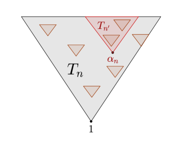
Figure 1: Schematic of the proof of Corollary 2. The outer triangle represents the genealogical tree $T_{n}$ of $Z(\tau_{n})$, and the small triangles are the subpopulations of size $j$ in ${\bf Y}^{(p_{n})}(\tau_{n})$. When $\alpha_{n}\sim n^{1-j/\ell}$, the subtree $T_{n^{\prime}}$ of $T_{n}$ rooted at the $\alpha_{n}$th individual has size $n^{\prime}\approx n^{j/\ell}$. Since $p_{n}\approx{(n^{\prime})}^{-1/j}$, Theorem 1 shows that within $T_{n^{\prime}}$, the number of subpopulations of size $j$ tends to infinity when $n\rightarrow\infty$. A fortiori, the same must hold for $\Delta^{n,p_{n}}(j)$.

Write $N^{n,p_{n}}_{|\alpha_{n}}(k)$ for the number of subpopulations of size $>k\in\mathbb{N}$ in the system ${\bf Y}^{(p)}$ stopped at time $\tau_{n}$, whose common ancestor is given by the $\alpha_{n}$th individual, and similarly, define $\Delta^{n,p_{n}}_{|\alpha_{n}}(k)$ by counting only the subpopulations of size equals $k$ that stem from individual $\alpha_{n}$. Obviously, $N^{n,p_{n}}_{|\alpha_{n}}(k)\leq N^{n,p_{n}}(k)$ and $\Delta^{n,p_{n}}_{|\alpha_{n}}(k)\leq\Delta^{n,p_{n}}(k)$. For $K>0$, we estimate

$$\mathbb{P}\left(\Delta^{n,p_{n}}(j)\geq K\right) \geq\mathbb{P}\left(\Delta^{n,p_{n}}_{\alpha_{n}}(j)\geq K\right)=\mathbb{P}\left(N^{n,p_{n}}_{|\alpha_{n}}(j-1)\geq K+N^{n,p_{n}}_{|\alpha_{n}}(j)\right)$$

$$\geq\mathbb{P}\left(N^{n,p_{n}}_{|\alpha_{n}}(j-1)\geq 2K\right)-\mathbb{P}\left(N^{n,p_{n}}_{|\alpha_{n}}(j)>K\right).$$ (18)

We will show that the first probability tends to $1$ for each choice of $K$, while the second can be made as small as we wish provided $K$ is sufficiently large.

For that purpose, we remark that conditionally on $Z_{\alpha_{n}}\left(\tau_{n}-\tau_{\alpha_{n}}\right)=m$, as a consequence of the dynamics, $N^{n,p_{n}}_{|\alpha_{n}}(k)$ for $k\in\mathbb{N}$ has same law as $N^{m,p_{n}}(k)$, the number of subpopulations exceeding $k$ in ${\bf Y}^{(p_{n})}(\tau_{m})$. Moreover, if $m,m^{\prime}\in\mathbb{N}$ with $m\leq m^{\prime}$, the variable $N^{m,p_{n}}(k)$ is stochastically dominated by $N^{m^{\prime},p_{n}}(k)$ (adding individuals can only increase subpopulations). Now fix $\varepsilon>0$. By (17), we find $n_{0}\in\mathbb{N}$ and $c_{1},C_{1}>0$ such that for all $n\geq n_{0}$, with $m_{n}=\lfloor c_{1}n^{j/\ell}\rfloor$ and $M_{n}=\lceil C_{1}n^{j/\ell}\rceil$, the event

$$A_{n}=\left\{Z_{\alpha_{n}}\left(\tau_{n}-\tau_{\alpha_{n}}\right)\in[m_{n},M_{n}]\right\}$$

has probability at least $1-\varepsilon$. We first look at the second probability in (4.1). By our observations from above, we have for $n\geq n_{0}$,

$$\mathbb{P}\left(N^{n,p_{n}}_{|\alpha_{n}}(j)>K\right)\leq\mathbb{P}\left(N^{n,p_{n}}_{|\alpha_{n}}(j)>K\,|\,A_{n}\right)+\varepsilon\leq\mathbb{P}\left(N^{M_{n},p_{n}}(j)>K\right)+\varepsilon.$$

Recalling that $p_{n}\sim an^{-1/\ell}\sim(C_{1}^{1/j}a)M_{n}^{-1/j}$, we deduce from Theorem 1 that for $K\in\mathbb{N}$,

$$\mathbb{P}\left(N^{M_{n},p_{n}}(j)>K\right)\rightarrow\mathbb{P}\left(\textup{Poi}(C_{1}j!a^{j})>K\right)\quad\textup{as }n\rightarrow\infty.$$

The right side is smaller than $\varepsilon$ provided $K$ is large enough. For the first probability in (4.1), we have similarly

$$\mathbb{P}\left(N^{n,p_{n}}_{|\alpha_{n}}(j-1)\geq 2K\right)\geq(1-\varepsilon)\mathbb{P}\left(N^{n,p_{n}}_{|\alpha_{n}}(j-1)\geq 2K\,|\,A_{n}\right)\geq(1-\varepsilon)\mathbb{P}\left(N^{m_{n},p_{n}}(j-1)\geq 2K\right).$$

By Theorem 1, $N^{m_{n},p_{n}}(j-1)\rightarrow\infty$ in probability as $n$ tends to infinity, hence the probability on the right tends to $1$ for each choice of $K$. Since $\varepsilon>0$ was arbitrary, this concludes the proof of the corollary. $\Box$

The next corollary of Theorem 1 characterizes the regime where unbounded subpopulations appear in the limit $n\rightarrow\infty$. For the sake of clarity, we write $\mathbb{P}_{p_{n}}$ for the law of the system ${\bf Y}^{(p_{n})}$.

Corollary 3.

Let $(p_{n})_{n}\subset[0,1]$. Then

$$\left[\lim_{K\rightarrow\infty}\liminf_{n\rightarrow\infty}\mathbb{P}_{p_{n}}\left(\exists i\in\mathbb{N}\textup{ such that }Y_{i}^{(p_{n})}(\tau_{n})>K\right)=1\right]\Leftrightarrow\left[p_{n}\,n^{1/\ell}\rightarrow\infty\textup{ for each }\ell\in\mathbb{N}\right].$$

If one of the statements fails, $\lim_{K\rightarrow\infty}\liminf_{n\rightarrow\infty}\mathbb{P}_{p_{n}}\left(\exists i\in\mathbb{N}\textup{ such that }Y_{i}^{(p_{n})}(\tau_{n})>K\right)=0.$

The proof is a direct application of Theorem 1 and left to the reader.

4.2 The regime $p_{n}\sim a\ln^{-1}n$

Parts $(a)$ and $(b)$ of Proposition 1 identify

$$p_{n}\sim\frac{a}{\ln n},\quad a>0\hbox{ fixed,}$$

as the regime in which the ancestral subpopulation becomes non-trivial. Its size however remains bounded. What are the sizes of the largest subpopulations that do appear? As a consequence of Theorem 3, we will see that if we shift the subpopulation sizes by $-(c_{1}\ln n+c_{2}\ln\ln n)$ for some explicit constants $c_{1},c_{2}>0$, then for any $\ell\in\mathbb{N}$ and any $\varepsilon>0$, we find $C=C(\ell,\varepsilon)$ such that the $\ell$ largest (shifted) sizes are contained in $[-C,C]$ with probability at least $1-\varepsilon$, provided $n$ is large enough.

While Theorem 3 holds true whenever $p_{n}\sim a\ln^{-1}n$, we will first prove Theorem 2, which provides a stronger result valid for the case $p_{n}=a\ln^{-1}n$. Here we will compute a correction $c_{3}$ of order one to the above shift, such that the number of subpopulations greater than $y_{n}=c_{1}\ln n+c_{2}\ln\ln n+c_{3}$ converges to a Poisson limit along all subsequences $(y_{n(m)})_{m}$ of $(y_{n})_{n}$, whose fractional part has a limit as $m$ tends to infinity. Theorem 3 then readily follows from adapting some estimates used in the proof of Theorem 2.

Before we give the precise formulation of our results, we need some preparation. For $a>0$, define

$$f_{a}(t)=1+t\ln(at)-\frac{1+at}{a}\ln(1+at),\quad t>0.$$ (19)

On $(0,\infty)$, $f_{a}$ is a smooth function with $f_{a}(t)\rightarrow 1$ as $t\rightarrow 0$ and $f_{a}(t)\rightarrow-\infty$ for $t\rightarrow\infty$. Moreover, since on $(0,\infty)$,

$$f^{\prime}_{a}(t)=\ln(at)-\ln(1+at)<0,$$

the function $f_{a}$ is strictly decreasing, and there is a unique $t^{\ast}=t^{\ast}(a)\in(0,\infty)$ for which $f_{a}(t^{\ast})=0$. See Figure 2.

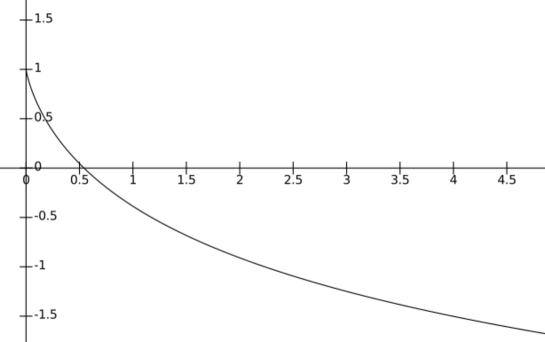
Figure 2: The function $f_{a}$ for $a=1$.

Now, for $a>0$ and $\lambda>0$ fixed and $t^{\ast}$ the root of $f_{a}$, put

$$y_{n}=t^{\ast}\ln n-\frac{1}{2f_{a}^{\prime}(t^{\ast})}\left(\ln\ln n+\ln\left(\frac{2\pi t^{\ast}}{\lambda^{2}(1+at^{\ast})}\right)\right)$$ (20)

We use the standard notation $\{y\}=y-\lfloor y\rfloor$ to denote the fractional part of a real $y\in\mathbb{R}$. As we will see in the following theorem, the barrier $y_{n}$ defines a precise threshold, in the following sense: Whenever $(y_{n(m)})_{m}$ is a subsequence of $(y_{n})_{n}$ such that $\lim_{m\rightarrow\infty}\{y_{n(m)}\}=:b\in[0,1)$ exists, then the number of subpopulations exceeding size $y_{n(m)}$ converges weakly to a Poisson$(\Lambda(a,b,\lambda))$-distributed random variable with intensity given by

$$\Lambda(a,b,\lambda)=\lambda\left(1+\frac{1}{at^{\ast}}\right)^{b}.$$ (21)

We will see in Corollary 4 that the restriction to subsequences with converging fractional part is actually necessary.

Theorem 2.

Assume $p_{n}=a\ln^{-1}n$ for some $a>0$. Let $\lambda>0$, and define $y_{n}=y_{n}(a,\lambda)$ as in (20). Let $(y_{n(m)})_{m}$ be a subsequence of $(y_{n})_{n}$ such that $\{y_{n(m)}\}\rightarrow b$ for some $b\in[0,1)$. Then, with $\Lambda(a,b,\lambda)$ as above, for $m\rightarrow\infty$,

$$N^{n(m),p_{n(m)}}(\lfloor y_{n(m)}\rfloor)\xrightarrow[]{(d)}{\textup{Poi}}\left(\Lambda(a,b,\lambda)\right).$$

Proof:   We again follow the strategy explained in Section 3. Recall that we require $p_{n}k_{n}\rightarrow 0$, and we will here choose $k_{n}=\lfloor\ln^{1/2}n\rfloor$. Putting $t_{n}=y_{n}/\ln n$, the first part of Lemma 3 and a small calculation show that as $n$ tends to infinity,

$${\rm I}(n,p_{n},\lfloor y_{n}\rfloor)\sim\sqrt{\frac{2\pi t_{n}}{1+at_{n}}}n\sqrt{\ln n}\frac{(at_{n})^{t_{n}\ln n}}{(1+at_{n})^{(a^{-1}+t_{n})\ln n}}\left(1+\frac{1}{at_{n}}\right)^{\{t_{n}\ln n\}}.$$

Taking the logarithm of the right hand side, we arrive at the expression

$$f_{a}(t_{n})\ln n+\frac{1}{2}\left(\ln\ln n+\ln\left(\frac{2\pi t_{n}}{1+at_{n}}\right)\right)+\{t_{n}\ln n\}\ln\left(1+\frac{1}{at_{n}}\right),$$ (22)

for $f_{a}$ as defined under (19). Obviously, $t_{n}=t^{\ast}+O(\frac{\ln\ln n}{\ln n})$, and by Taylor’s formula,

$$f_{a}(t_{n})=f_{a}^{\prime}(t^{\ast})(t_{n}-t^{\ast})+O\left(\left(\frac{\ln\ln n}{\ln n}\right)^{2}\right),$$

so that

$$f_{a}(t_{n})\ln n=-\frac{1}{2}\left(\ln\ln n+\ln\left(\frac{2\pi t_{n}}{\lambda^{2}(1+at_{n})}\right)\right)+o(1).$$

Taking exponentials, (22) and the last display show that for $m$ tending to infinity,

$${\rm I}\left(n(m),p_{n(m)},\lfloor y_{n(m)}\rfloor\right)\sim\Lambda(a,b,\lambda).$$

We next control the error terms $\Sigma_{1}^{n,p_{n}}$, $\Sigma_{2}^{n,p_{n}}$ and $\Sigma_{3}^{n,p_{n}}$. First, recalling that $\overline{\beta}(n)\leq\ln n+o(1)$, we have for $n$ sufficiently large,

$$\Sigma_{1}^{n,p_{n}}(\lfloor y_{n}\rfloor) =2k_{n}\left(1-\exp\left(-p_{n}(\overline{\beta}(n)+\ln^{2}(k_{n}))\right)\right)^{\lfloor y_{n}\rfloor}$$

$$\leq 2(\ln^{1/2}n)\left(1-\exp(-2a)\right)^{\lfloor y_{n}\rfloor}=o(1).$$

In particular,

$$\mathbb{E}\left[\overline{S}^{n(m),p_{n(m)}}(\lfloor y_{n(m)}\rfloor)\right]\leq\Lambda(a,b,\lambda)+o(1),$$

and, with Cauchy-Schwarz and Remark 2, $\Sigma_{2}^{n(m),p_{n(m)}}(\lfloor y_{n(m)}\rfloor)=o(1)$. Finally,

$$\Sigma_{3}^{n,p_{n}}(\lfloor y_{n}\rfloor) \leq n\int_{\underline{\beta}(n)-\overline{\beta}(2k_{n})}^{\infty}\left(1-{\rm e}^{-p_{n}s}\right)^{\lfloor y_{n}\rfloor}{\rm e}^{-s}{\textup{d}}s$$

$$\leq\frac{1}{n}+n\left(1-{\rm e}^{-2a}\right)^{\lfloor y_{n}\rfloor}\int_{\ln n-2\ln\ln n}^{2\ln n}{\rm e}^{-s}{\textup{d}}s=o(1),$$

so that as $m\rightarrow\infty$,

$$\mathbb{E}\left[\underline{S}^{n(m),p_{n(m)}}(\lfloor y_{n(m)}\rfloor)1\mkern-6.0mu1_{E_{n(m)}}\right]\sim\mathbb{E}[N^{n(m),p_{n(m)}}(\lfloor y_{n(m)}\rfloor)1\mkern-6.0mu1_{E_{n(m)}}] \sim\mathbb{E}\left[\overline{S}^{n(m),p_{n(m)}}(\lfloor y_{n(m)}\rfloor)\right]$$

$$\sim\Lambda(a,b,\lambda).$$

The condition under Step $2$ is fulfilled as well, see the estimate for $\Sigma_{1}^{n,p_{n}}$. Performing Step $3$, it follows that $N^{n(m),p_{n(m)}}(\lfloor y_{n(m)}\rfloor)$ converges to a Poisson$(\Lambda(a,b,\lambda))$ random variable. $\Box$

Theorem 2 implies the following remarkable weak convergence along subsequences for the size $C_{\ast}^{n,p_{n}}$ of the largest subpopulation at time $\tau_{n}$. For $a>0$, $r\in\mathbb{R}$ and $t^{\ast}$ the root of $f_{a}$, put

$$\lambda_{a,r}=\left(\frac{2\pi t^{\ast}}{1+at^{\ast}}\right)^{1/2}{\rm e}^{-r/2}.$$

Corollary 4.

Let $a>0$, $p_{n}=a\ln^{-1}n$ and $r\in\mathbb{R}$. Define $\lambda_{a,r}$ as above, and $y_{n}=y_{n}(a,\lambda_{a,r})$ in terms of $\lambda_{a,r}$ as in (20). Let $(y_{n(m)})_{m}$ be any subsequence of $(y_{n})_{n}$ such that $\{y_{n(m)}\}\rightarrow b$ for some $b\in[0,1)$. Then, for $m\rightarrow\infty$, with $\mu=\ln\left(2\pi/a^{2b}\right)+(1-2b)\ln\left(t^{\ast}/(1+at^{\ast})\right)$,

$$\mathbb{P}\left(C_{\ast}^{n(m),p_{n(m)}}-t^{\ast}\ln n(m)+\frac{1}{2f_{a}^{\prime}(t^{\ast})}\ln\ln n(m)\leq r\right)\rightarrow\exp\left(-{\rm e}^{-(r-\mu)/2}\right).$$

Proof:   The probability on the left hand side is equal to

$$\mathbb{P}\left(C_{\ast}^{n(m),p_{n(m)}}\leq\lfloor y_{n(m)}\rfloor\right)=\mathbb{P}\left(N^{n(m),p_{n(m)}}(\lfloor y_{n(m)}\rfloor)=0\right)\sim\mathbb{P}\left({\textup{Poi}}(\Lambda(a,b,\lambda_{a,r}))=0\right),$$

with $\Lambda(a,b,\lambda_{a,r})$ defined as in (21). The last asymptotics holds thanks to Theorem 2. The claim follows. $\Box$

Remark 3.

The limit expression on the right hand side in the above corollary is the distribution function of the Gumbel law with location parameter $\mu$ and scale parameter $2$. In view of our heuristics explained in Section 2.3 and of what is known about the maximum of $n$ independent geometrically distributed random variables, it should not come as a surprise that a Gumbel distribution appears in the limit for the recentered size of the largest subpopulation. Since $C_{\ast}^{n,p_{n}}$ is a discrete random variable and the Gumbel law is a continuous distribution, convergence along the full sequence cannot hold.

It is instructive to compare our previous two results with Theorem 5.10 and Corollary 5.11 of [11] for the Erdős-Rényi random graph model.

From the proof of Theorem 2, we easily derive that in the general case $p_{n}\sim a\ln^{-1}n$, the sizes of the largest subpopulations are concentrated around

$$b_{n}=t^{\ast}\ln n-\frac{1}{2f_{a}^{\prime}(t^{\ast})}\ln\ln n.$$ (23)

Theorem 3.

Assume $p_{n}\sim a\ln^{-1}n$ for some $a>0$. Define $b_{n}=b_{n}(a)$ as in (23), and let $(x_{n})_{n}$ be a sequence of positive integers. Then the following holds as $n\rightarrow\infty$.

1. If $(x_{n}-b_{n})\gg 1$, then $N^{n,p_{n}}(x_{n})\rightarrow 0.$

2. If $(b_{n}-x_{n})\gg 1$, then $N^{n,p_{n}}(x_{n})\rightarrow\infty.$

Proof:   We only have to adapt the estimates given in the proof of Theorem 2, so we will only sketch the necessary modifications. We again choose $k_{n}=\lfloor\ln^{1/2}n\rfloor$. We treat $(a)$ and $(b)$ together, and in this regard, we note that for $(b)$, by monotonicity of $N^{n,p_{n}}(x)$ we can assume that $x_{n}\gg\ln\ln n$. With $y_{n}$ everywhere replaced by $x_{n}$, we deduce from (22) that if $(x_{n}-b_{n})\gg 1$, then ${\rm I}(n,p_{n},x_{n})\rightarrow-\infty$, whereas if $(b_{n}-x_{n})\gg 1$, then ${\rm I}(n,p_{n},x_{n})\rightarrow\infty$. The error term $\Sigma_{1}^{n,p_{n}}(x_{n})$ is seen to be of order $o(1)$ with exactly the same argument as in the proof of Theorem 2, and so is the error term $\Sigma_{3}^{n,p_{n}}(x_{n})$, using here that $x_{n}\gg\ln\ln n$.

Now if $(x_{n}-b_{n})\gg 1$, we have by Markov’s inequality and (12),

$$\mathbb{P}\left(N^{n,p_{n}}(x_{n})\geq 1\right)\leq\mathbb{E}\left[\overline{S}^{n,p_{n}}(x_{n})\right]+o(1)=o(1),$$

and if $(b_{n}-x_{n})\gg 1$, then, as in the second part of the proof of Theorem 1, for any $K\in\mathbb{N}$,

$$\mathbb{P}\left(N^{n,p_{n}}(x_{n})\geq K\right)\geq\mathbb{P}\left(\underline{S}^{n,p_{n}}(x_{n})\geq K\right)-o(1).$$

The probability on the right tends to $1$ by an appeal to Lemma 5. $\Box$

4.3 The regime $\ln^{-1}n\ll p_{n}\ll 1$.

In the regime $p_{n}\gg 1/\ln n$, the ancestral subpopulation grows like $n^{p_{n}}$, see part $(c)$ of Proposition 1. As we shall prove in the following theorem, when $1/\ln n\ll p_{n}\ll 1$, the sizes of the largest subpopulations are to first order given by ${\rm e}^{-1}p_{n}^{-1}n^{p_{n}}$. For the case $\ln\ln n/\ln n\leq p_{n}\ll 1$ and $\lambda>0$, we will show that the number of subpopulations greater than

$$x_{n}=x_{n}(p_{n},\lambda)=\Bigl{\lfloor}{\left(\lambda^{-1}\sqrt{2\pi p_{n}^{-1}}\right)}^{p_{n}}{\rm e}^{-1}p^{-1}_{n}n^{p_{n}}\Bigr{\rfloor}$$ (24)

is asymptotically Poisson$(\lambda)$-distributed. Note that as $n\rightarrow\infty$, $g_{\lambda}(p_{n})=(\lambda^{-1}\sqrt{2\pi p_{n}^{-1}})^{p_{n}}\sim 1$, cf. Figure 3.

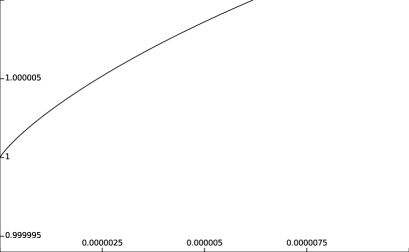
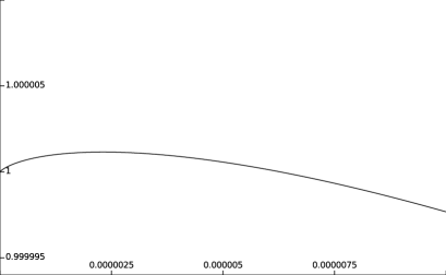
Figure 3: The function $g_{\lambda}(p)$ on $[0,10^{-5}]$ for $\lambda=200$ (left side) and $\lambda=1000$ (right side).

As it will become clear from the proof, we require $p_{n}\geq\ln\ln n/\ln n$ (and not merely $p_{n}\gg 1/\ln n$) only to simplify the calculation; without this assumption, the exact behavior of $p_{n}$ has to be taken into account more carefully.

Theorem 4.

Assume $\ln^{-1}n\ll p_{n}\ll 1$. Then the following holds as $n\rightarrow\infty$.

1. If $u>{\rm e}^{-1}$, then $N^{n,p_{n}}(\lfloor up_{n}^{-1}n^{p_{n}}\rfloor)\xrightarrow[]{(p)}0$. If $u<{\rm e}^{-1}$, then $N^{n,p_{n}}(\lfloor up_{n}^{-1}n^{p_{n}}\rfloor)\xrightarrow[]{(p)}\infty$.

2. Assume additionally $p_{n}\geq\ln\ln n/\ln n$ for large $n$. Then, with $x_{n}$ as in (24),

   $$N^{n,p_{n}}(x_{n})\xrightarrow[]{(d)}{\textup{Poi}}(\lambda).$$

Proof:   We work with the choice $k_{n}=\lfloor p_{n}^{-1/2}\rfloor$ and follow the steps of the strategy presented in Section 3. Since our proof is similar to the proofs of Theorem 1 and Theorem 2, we do not provide every detail.

We fix a real number $u>0$ and let $y_{n}=\lfloor up_{n}^{-1}n^{p_{n}}\rfloor$, $n\in\mathbb{N}$. For the main term ${\rm I}(n,p_{n},y_{n})$, Lemma 3 shows

$${\rm I}(n,p_{n},y_{n})\sim\sqrt{2\pi}\,n\frac{(1/p_{n})^{1/p_{n}+1/2}\,y_{n}^{y_{n}+1/2}}{(1/p_{n}+y_{n})^{1/p_{n}+y_{n}+1/2}}.$$ (25)

Note that since $p_{n}\gg 1/\ln n$, we have $p_{n}y_{n}\rightarrow\infty$ as $n\rightarrow\infty$. By Taylor’s formula,

$$\ln\left(\frac{1}{p_{n}}+y_{n}\right)=\ln(y_{n})+\frac{1}{p_{n}y_{n}}+O\left(\frac{1}{p^{2}_{n}y^{2}_{n}}\right).$$

From the last display, we deduce after a short calculation that the logarithm of the right hand side of (25) behaves asymptotically like

$$\frac{1}{2}\ln(2\pi)+\ln n-\left(\frac{1}{p_{n}}+\frac{1}{2}\right)\ln p_{n}-\frac{1}{p_{n}}\ln(y_{n})-\frac{1}{p_{n}}+O\left(\frac{1}{p^{2}_{n}y_{n}}\right)$$

$$\quad\quad\quad\quad=-\frac{1}{p_{n}}\left(1+\ln(u)+O(n^{-p_{n}})\right)-\frac{1}{2}\ln p_{n}+\frac{1}{2}\ln(2\pi).$$ (26)

In particular, if $u>{\rm e}^{-1}$, then the right hand side diverges to $-\infty$, whereas if $u<{\rm e}^{-1}$, it diverges to $+\infty$. Consequently, ${\rm I}(n,p_{n},y_{n})\rightarrow 0$ in the first and ${\rm I}(n,p_{n},y_{n})\rightarrow\infty$ in the second case. In order to finish the proof of $(a)$, it remains to convince ourselves that the error terms $\Sigma_{1}^{n,p_{n}}(y_{n})$ and $\Sigma_{3}^{n,p_{n}}(y_{n})$ do not contribute when $n$ tends to infinity. For the first one, we have

$$\Sigma_{1}^{n,p_{n}}(y_{n})\leq 2p_{n}^{-1/2}\left(1-\exp\left(-p_{n}(\overline{\beta}(n)+\ln^{2}(\lfloor p_{n}^{-1/2}\rfloor))\right)\right)^{y_{n}}.$$

Since $\overline{\beta}(n)\leq\ln n+o(1)$, we see from taking logarithms that $\Sigma_{1}^{n,p_{n}}(y_{n})=o(1)$, as wanted. The error term $\Sigma_{3}^{n,p_{n}}(y_{n})$ is readily seen to be of order $o(1)$ as well, and the claims under $(a)$ now follow from the same arguments as in the proof of Theorem 3 (or Theorem 1).

We turn to $(b)$ and fix $\lambda>0$. If $p_{n}\geq\ln\ln n/\ln n$ for $n$ large, then, with $x_{n}$ defined as in (24),

$$O\left(\frac{1}{p_{n}n^{p_{n}}}\right)=o(1).$$

Performing the above calculation with $y_{n}$ replaced by $x_{n}$ and $u$ by

$$u_{n}={\left(\lambda^{-1}\sqrt{2\pi p_{n}^{-1}}\right)}^{p_{n}}{\rm e}^{-1},$$

we deduce from (4.3) that the logarithm of right side in (25) behaves as $\ln\lambda+o(1)$, and thus

$${\rm I}(n,p_{n},x_{n})\sim\lambda.$$

Part $(b)$ now follows from the same line of reasoning as in the proof of Theorem 2, using that all the error terms $\Sigma_{i}^{n,p_{n}}(x_{n})$, $i=1,2,3$, are of order $o(1)$. $\Box$

5 Subcritical percolation on random recursive trees

In this final section, we make the precise link between the population system ${\bf Y}^{(p)}$ defined in Section 2 and percolation on random recursive trees.

A recursive tree with vertex set $[n]=\{1,\ldots,n\}$ is a tree rooted at $1$ with the property that the labels along the unique path from the root to any other vertex form an increasing sequence. A tree chosen uniformly at random among all these $(n-1)!$ recursive trees is called random recursive tree and denoted $T_{n}$. The study of Bernoulli bond percolation on large random recursive trees can be traced back to the analysis of an algorithm for isolating the root by Meir and Moon [19]; see also Drmota et al. [13] , Iksanov and Möhle [15] and Kuba and Panholzer [17] for more recent developments in this direction. It further plays a key role in the construction of the Bolthausen-Sznitman coalescent by Goldschmidt and Martin [14].

We choose $p=p_{n}\in(0,1)$ and write $C_{1}^{n,p},C_{2}^{n,p},\ldots$ for the percolation clusters of a Bernoulli bond percolation on $T_{n}$ with parameter $p$. That is, we erase each edge of $T_{n}$ with probability $1-p$ and independently of each other, and enumerate the connected components according to the increasing order of the label of their root vertex (i.e. their vertex with the smallest label).

We use the convention that $C_{i}^{n,p}=\emptyset$ if there are less than $i$ connected components after percolation on $T_{n}$. With our ordering, $C_{1}^{n,p}$ always represents the root cluster containing $1$; $C_{2}^{n,p}$ is the cluster rooted at the smallest vertex which does not belong to the root cluster $C_{1}^{n,p}$, and so on. We write $|C_{i}^{n,p}|$ for the number of vertices of $C_{i}^{n,p}$. Then the following holds.

Lemma 6.

Let $p\in[0,1]$. The families $(|C_{1}^{n,p}|,|C_{2}^{n,p}|,\ldots)$ and $(Y_{1}^{(p)}(\tau_{n}),Y_{2}^{(p)}(\tau_{n}),\ldots)$ have the same law.

Proof:   We construct percolation on a random recursive tree as a growth process in continuous time as follows. At time $t=0$, we start from the singleton $\{1\}$. Given percolation with parameter $p$ on a random recursive tree on $[k]$, $k\geq 1$, has been constructed, we equip each vertex $i\in[k]$ with an independent exponential clock $\mathcal{E}_{i}$ of parameter $1$. At time $\min_{i=1,\ldots,k}\mathcal{E}_{i}$, we flip a coin with heads probability $p$. If head shows up, we attach a vertex labeled $k+1$ to the vertex with label arg$\min_{i=1,\ldots,k}\mathcal{E}_{i}$. Otherwise, we add vertex $k+1$ to the system without connecting it to any other vertex. It follows from the construction of random recursive trees and the independence of the coin flips that we observe at the instant when the $n$th vertex is incorporated a Bernoulli bond percolation on $T_{n}$ with parameter $p$. Moreover, if we keep track of the sizes ${\bf C}^{(p)}(t)=(|C_{1}^{(p)}(t)|,|C_{2}^{(p)}(t)|,\ldots)$ of the growing percolation clusters, where $|C_{i}^{(p)}(t)|$ stores the size of the $i$th cluster at time $t$ and clusters are ordered according to their birth times, we obtain a Markov chain with initial state ${\bf C}^{(p)}(0)=(1,0,\ldots)$ and transition rates at time $t\geq 0$ for $c_{1},\ldots,c_{k}\in\mathbb{N}$ given by

$$(c_{1},\ldots,c_{k},0,\ldots) \mapsto(c_{1},\ldots,c_{k},1,0,\ldots)\quad\textup{at rate }(1-p)(c_{1}+\ldots+c_{k}),$$

$$(c_{1},\ldots,c_{k},0,\ldots) \mapsto(c_{1},\ldots,c_{i-1},c_{i}+1,c_{i+1},\ldots,c_{k},0,\ldots)\quad\textup{at rate }pc_{i}.$$

From the very construction of ${\bf Y}^{(p)}$, it follows that the processes $({\bf Y}^{(p)}(t):t\geq 0)$ and $({\bf C}^{(p)}(t):t\geq 0)$ grow according to the same dynamics, and the statement follows. $\Box$

If we think of the individuals of ${\bf Y}^{(p)}$ as being labeled $1,2,\ldots$, according to the increasing order of their birth times, there is in fact a one-to-one correspondence between subpopulations and clusters that respects the genealogy, as illustrated by Figure 4.

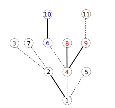
Figure 4: The genealogical tree of a Yule process with mutation, stopped after the birth of the $11$th individual. Subpopulations of different genetic types have different colors, and the edges connecting mutants to their parent are represented by dashed lines. Alternatively, the subpopulations can be viewed as the clusters of a Bernoulli bond percolation on a recursive tree on $\{1,\ldots,11\}$.

With the above lemma at hand, the results from Section 4 have a direct interpretation in terms of clusters stemming from a percolation on $T_{n}$ with parameter $p_{n}$. For example, Corollary 3 gives a necessary and sufficient condition on the percolation parameter $p_{n}$ such that in the limit $n\rightarrow\infty$, clusters of unbounded size appear.

More generally, the strategy developed in Section 3 gives a concise tool to decide whether for a given percolation sequence $p_{n}\rightarrow 0$ and thresholds $x_{n}$, there are clusters of a size of order $x_{n}$, and if so, how many. Indeed, as exemplified in Section 4, basically one only has to check the asymptotic behavior of the expression ${\rm I}(n,p_{n},x_{n})$ introduced below Lemma 2.

This work completes the study of percolation on random recursive trees initiated in [6], where percolation with supercritical parameter $p_{n}\sim 1-a/\ln n$, $a>0$ fixed, is studied. In [7], non-Gaussian fluctuations of the root cluster were proved, and the analysis of percolation clusters was extended in [4] to all regimes $p_{n}\rightarrow 1$. The works [6, 4] do additionally contain information on the genealogy of clusters (and not merely on their sizes), a type of question we did not investigate here.

As a common feature when $p_{n}\rightarrow 1$, the root cluster containing $1$ has size $\sim n^{p_{n}}$, while the sizes of the next largest clusters are of order $(1-p_{n})n^{p_{n}}$. This motivated a sub-classification of regions into weakly supercritical [$1/\ln n\ll 1-p_{n}\ll 1$] when $|C_{1}^{n,p_{n}}|\ll n$, supercritical [$1-p_{n}\sim t/\ln n$, $t>0$ fixed] when $|C_{1}^{n,p_{n}}|\sim{\rm e}^{-t}n$, and strongly supercritical [$1-p_{n}\ll 1/\ln n$] when $|C_{1}^{n,p_{n}}|\sim n$.

The regime of constant $p\in(0,1)$ may best be termed “critical”, since in this case, the root cluster loses its dominating role (with respect to the size). Some results can be found in [20] and [5], although the motivation there is somehow different. For similar reasons, we term the regime $p=p_{n}\rightarrow 0$ considered here “subcritical”. The classification into different regimes draws on the terminology which is usually used to describe the Erdős-Rényi random graph model (see, e.g., [2]).

We stress that there are other natural families of trees which can be grown according to a probabilistic evolution algorithm, like, e.g., scale-free random trees or $b$-ary random increasing trees. Indeed, branching systems with mutations were used in [8] to study percolation on scale-free random trees when $p_{n}\sim a/\ln n$, and in a similar fashion by Berzunza in [9] for $b$-ary random increasing trees. In the case of random recursive trees, the underlying population system is particularly simple, so we restricted our discussion of the subcritical regime to these trees, but we certainly expect similar results to hold true for other classes of increasing tree families.

Appendix A Proof of Lemma 1

In this appendix, we will construct an event $E_{n}$ with the “good” properties specified in Lemma 1. We first collect some properties of Yule processes.

A.1 Some properties of Yule processes

For $p\in[0,1]$, denote by $Y^{(p)}=(Y^{(p)}(t):t\geq 0)$ a Yule process with birth rate $p$ per unit population size. Given $y\in\mathbb{N}$, write $\mathbb{P}_{y}$ for its law under which $\mathbb{P}_{y}(Y^{(p)}(0)=y)=1$, and similarly $\mathbb{E}_{y}$ for its expectation. It is well-known that $W^{(p)}(t)={\rm e}^{-pt}Y^{(p)}(t)$, $t\geq 0$, is a square-integrable martingale. Under $\mathbb{P}_{y}$ and for $p>0$, its terminal value $W^{(p)}(\infty)$ is distributed as a sum of $y$ standard exponentials and follows thus the Gamma$(y,1)$-law. Note that Doob’s inequality applied to the square-integrable martingale $W^{(p)}(t)-y$ gives

$$\mathbb{E}_{y}\left[\sup_{t\geq 0}\big{|}W^{(p)}(t)-W^{(p)}(0)\big{|}^{2}\right]\leq 4\mathbb{E}_{y}\left[|W^{(p)}(\infty)-W^{(p)}(0)|^{2}\right]=4y.$$ (27)

We now work in the setting of Section 2. Recall the definition of the process $T^{(p)}=(T^{(p)}(t):t\geq 0)$ counting the number of different genetic types in the population system ${\bf Y}^{(p)}$, starting from $T^{(p)}(0)=1$. For $i\in\mathbb{N}$, $\tau_{i}=\inf\left\{t\geq 0:Z(t)=i\right\}$ denotes the birth time of the $i$th individual in the system ${\bf Y}^{(p)}$ (counting both clones and mutants), with $Z$ denoting the underlying standard Yule process. The time $b_{i}^{(p)}$ denotes the first time when an individual of genetic type $i$ appears, i.e., the $b_{i}^{(p)}$’s are the jump times of $T^{(p)}(t)$. We need the following control over $T^{(p)}$.

Lemma 7.

Let $p\in(0,1)$. For $k\in\mathbb{N}$, let $\mathbb{P}_{|k}$ be the conditional law given $\{\tau_{k}=b_{k}^{(p)}\}$ (i.e. the first $k-1$ children are all mutants), and let $\mathbb{E}_{|k}$ be its expectation. For every $t\geq 0$, we have

$$\mathbb{E}_{|k}\left[\sup_{0\leq s\leq t}\left|T^{(p)}(\tau_{k}+s)-\left(k+\int_{\tau_{k}}^{\tau_{k}+s}(1-p)Z(r){\textup{d}}r\right)\right|^{2}\right]\leq 4(1-p)k({\rm e}^{t}-1),$$

and

$$\mathbb{E}_{|k}\left[\sup_{s\geq t}{\rm e}^{-5s/3}\left|T^{(p)}(\tau_{k}+s)-\left(k+\int_{\tau_{k}}^{\tau_{k}+s}(1-p)Z(r){\textup{d}}r\right)\right|^{2}\right]\leq 324(1-p)k\,{\rm e}^{-2t/3}.$$

Proof:   Let $\mathcal{F}_{t}$ denote the natural filtration generated by the process $({\bf Y}^{(p)}(t):t\geq 0)$. Both processes $T^{(p)}$ and $Z$ are $\mathcal{F}_{t}$-adapted, and $\tau_{k}$ is a stopping time. We work now under the probability measure $\mathbb{P}_{|k}$. From the strong Markov property and the dynamics of ${\bf Y}^{(p)}$ described above, we see that $M^{(p)}(s)=T^{(p)}(\tau_{k}+s)-(k+\int_{\tau_{k}}^{\tau_{k}+s}(1-p)Z(r){\textup{d}}r)$ is a martingale with $M^{(p)}(0)=0$. Its quadratic variation is given by $[M^{(p)}](s)=T^{(p)}(\tau_{k}+s)-k$, and its second moment takes the form

$$\mathbb{E}_{|k}\left[|M^{(p)}(s)|^{2}\right] =\mathbb{E}_{|k}\left[[M^{(p)}](s)\right]=\mathbb{E}_{|k}\left[T^{(p)}(\tau_{k}+s)\right]-k$$

$$=\mathbb{E}_{|k}\left[\int_{\tau_{k}}^{\tau_{k}+s}(1-p)Z(r){\textup{d}}r\right]=\int_{0}^{s}(1-p)\mathbb{E}[Z(\tau_{k}+r)]{\textup{d}}r=(1-p)k({\rm e}^{t}-1).$$

For the last equality, we used the strong Markov property, which entails that $(Z(\tau_{k}+r):r\geq 0)$ is independent of $\mathcal{F}_{\tau_{k}}$ and distributed as a standard Yule process started from $k$ individuals. An appeal to Doob’s inequality gives

$$\mathbb{E}_{|k}\left[\sup_{0\leq s\leq t}|M^{(p)}(s)|^{2}\right]\leq 4\mathbb{E}_{|k}\left[|M^{(p)}(t)|^{2}\right]=4(1-p)k({\rm e}^{t}-1).$$

For the second statement, we bound for every $n\in\mathbb{N}$

$$\sup_{n\leq s<n+1}{\rm e}^{-5s/6}|M^{(p)}(s)|\leq{\rm e}^{-5n/6}\sup_{n\leq s<n+1}|M^{(p)}(s)|.$$

By Doob’s inequality, see the first part, the $L^{2}$-norm of the right side (with respect to the conditional measure $\mathbb{P}_{|k}$) is bounded by

$${\rm e}^{-5n/6}\left\|\sup_{n\leq s<n+1}|M^{(p)}(s)|\right\|_{2}\leq 2{\rm e}^{-5n/6}\sqrt{(1-p)k{\rm e}^{n+1}}\leq 2{\rm e}^{1/2}\sqrt{(1-p)k}\,{\rm e}^{-n/3}.$$

Thus, summing over $n$ and applying the triangle inequality,

$$\left\|\sup_{s\geq t}{\rm e}^{-5s/6}|M^{(p)}(s)|\right\|_{2}\leq 2{\rm e}^{1/2}\sqrt{(1-p)k}\sum_{n\geq\lfloor t\rfloor}{\rm e}^{-n/3}\leq 18\sqrt{(1-p)k}\,{\rm e}^{-t/3}.$$

Squaring both sides, the claim follows. $\Box$

We finally turn to the construction of an event $E_{n}=E_{n,p_{n},k_{n}}$ that satisfies the properties of Lemma 1.

Proof of Lemma 1:    We assume $p_{n}\rightarrow 0$ and fix any sequence of integers $k_{n}\in\mathbb{N}$ satisfying $k_{n}\rightarrow\infty$ and $k_{n}p_{n}\rightarrow 0$ as $n\rightarrow\infty$. Concerning property $(a)$ in Lemma 1, we first note that since each new-born child is a mutant with probability $1-p_{n}$, we have

$$\mathbb{P}\left(\tau_{k_{n}}=b_{k_{n}}^{(p_{n})}\right)=(1-p_{n})^{k_{n}-1}=1-o(1).$$

Moreover, by (1), we also have $\mathbb{P}(\tau_{k_{n}}<(\ln k_{n})^{2})=1-o(1)$, so that the event

$$E_{n}^{1}=\left\{\tau_{k_{n}}=b_{k_{n}}^{(p_{n})}\right\}\cap\left\{\tau_{k_{n}}<(\ln k_{n})^{2}\right\}$$

has probability $1-o(1)$ as $n$ tends to infinity.

We turn to property $(b)$. Since conditionally on $\tau_{k_{n}}$, $(Z(t+\tau_{k_{n}}):t\geq 0)$ is a Yule process started from $k_{n}$ individuals, we obtain from (27) and Chebycheff’s inequality

$$\mathbb{P}\left(\sup_{t\geq 0}\big{|}{\rm e}^{-t}Z(t+\tau_{k_{n}})-k_{n}|>k_{n}^{2/3}\right)\leq\frac{4}{k_{n}^{1/3}}.$$

In particular, if we let

$$E_{n}^{2}=\left\{(1-k_{n}^{-1/3})k_{n}{\rm e}^{t}\,\leq Z(\tau_{k_{n}}+t)\,\leq(1+k_{n}^{-1/3})k_{n}{\rm e}^{t}\quad\textup{for all }t\geq 0\right\},$$

then $\mathbb{P}(E_{n}^{2})\geq 1-4/k_{n}^{1/3}=1-o(1)$.

Finally, for property $(c)$ we need control over $(T^{(p)}(t):t\geq 0)$. In this regard, Lemma 7 in combination with Chebycheff’s inequality shows that conditionally on $\{\tau_{k_{n}}=b_{k_{n}}^{(p_{n})}\},$ the event

$$E_{n}^{3}=\left\{\left|T^{(p_{n})}(\tau_{k_{n}}+t)-\left(k_{n}+\int_{\tau_{k_{n}}}^{\tau_{k_{n}}+t}(1-p_{n})Z(r){\textup{d}}r\right)\right|\leq{\rm e}^{5t/6}k_{n}^{2/3}\quad\textup{for all }t\geq 0\right\}$$

has probability at least $1-324/k_{n}^{1/3}$. On $E_{n}^{2}\cap E_{n}^{3}$, we note that for $n$ sufficiently large, recalling that $p_{n}k_{n}\rightarrow 0$,

$$T^{(p_{n})}(\tau_{k_{n}}+t)\geq k_{n}+(1-p_{n})(1-k_{n}^{-1/3})k_{n}\int_{0}^{t}{\rm e}^{r}{\textup{d}}r-{\rm e}^{5t/6}k_{n}^{2/3}\geq(1-3k_{n}^{-1/3})k_{n}{\rm e}^{t},$$

and similarly

$$T^{(p_{n})}(\tau_{k_{n}}+t)\leq(1+3k_{n}^{-1/3})k_{n}{\rm e}^{t}.$$

Setting

$$E_{n}=E_{n}^{1}\cap E_{n}^{2}\cap E_{n}^{3},$$

we have constructed an event of probability $1-o(1)$ on which for $n$ sufficiently large, $(a)$, $(b)$ and $(c)$ in the statement of Lemma 1 are fulfilled. $\Box$

References

- [1] Aldous, D. Probability approximations via the Poisson clumping heuristic. Springer-Verlag, New York, (1989).
- [2] Alon, N., Spencer, J. The probabilistic method. Wiley, Third Edition (2008).
- [3] Athreya, K.B., Ney, P.E. Branching Processes. Dover Books on Mathematics (2004).
- [4] Baur, E. Percolation on random recursive trees. Preprint (2014), available at arXiv:1407.2508. To appear in Random Struct. Algor.
- [5] Baur, E., Bertoin, J. The fragmentation process of an infinite recursive tree and Ornstein-Uhlenbeck type processes. Electron. J. Probab. 20 (98) (2015), 1–20.
- [6] Bertoin, J. Sizes of the largest clusters for supercritical percolation on random recursive trees. Random Struct. Algor. 44 (1) (2014), 1098–2418.
- [7] Bertoin, J. On the non-Gaussian fluctuations of the giant cluster for percolation on random recursive trees. Electron. J. Probab. 19 (2014), no. 24, 1–15.
- [8] Bertoin, J., Uribe Bravo, G. Supercritical percolation on large scale-free random trees. Ann. Appl. Probab. 25 (1) (2015), 81–103.
- [9] Berzunza, G. Yule processes with rare mutation and their applications to percolation on b-ary trees. Electron. J. Probab. 20 (2015), 1–23.
- [10] Billinsgley, P. Convergence of Probability Measures. Second edition. Wiley series in Probability and Statistics (1999).
- [11] Bollobás, B. Random Graphs. Second edition. Cambridge University Press (2001).
- [12] Dobrow, R. P., Smythe R. T. Poisson approximations for functionals of random trees. Random Struct. Algor., 9 (1-2) (1996), 79–92.
- [13] Drmota, M., Iksanov, A., Möhle, M. and Rösler, U. A limiting distribution for the number of cuts needed to isolate the root of a random recursive tree. Random Struct. Algor. 34 (3) (2009), 319–336.
- [14] Goldschmidt, C. and Martin, J. B. Random recursive trees and the Bolthausen-Sznitman coalescent. Electron. J. Probab. 10 (2005), 718–745.
- [15] Iksanov, A. and Möhle, M. A probabilistic proof of a weak limit law for the number of cuts needed to isolate the root of a random recursive tree. Electron. Comm. Probab. 12 (2007), 28–35.
- [16] Klebaner, F. C. Introduction to Stochastic Calculus with Applications. Imperial College Press, 2nd edition (2005).
- [17] Kuba, M. and Panholzer, A. Multiple isolation of nodes in recursive trees. Online J. Anal. Comb. 9, (2014). Available at http://www.math.rochester.edu/ojac/vol9/98.pdf
- [18] Le Cam, L. An approximation theorem for the Poisson binomial distribution. Pacific J. Math. 10 (1960), 1181–1197.
- [19] Meir, A. and Moon, J. W. Cutting down recursive trees. Math. Biosci. 21 (1974), 173–181.
- [20] Möhle, M. The Mittag-Leffler process and a scaling limit for the block counting process of the Bolthausen-Sznitman coalescent. Lat. Am. J. Probab. Math. Stat. 12 (1) (2015), 35–53.