Ricci de Turck flow on singular manifolds

Abstract.

In this paper we prove local existence of a Ricci de Turck flow starting at a space with incomplete edge singularities and flowing for a short time within a class of incomplete edge manifolds. We derive regularity properties for the corresponding family of Riemannian metrics and discuss boundedness of the Ricci curvature along the flow. For Riemannian metrics that are sufficiently close to a flat incomplete edge metric, we prove long time existence of the Ricci de Turck flow. Under certain conditions, our results yield existence of Ricci flow on spaces with incomplete edge singularities. The proof works by a careful analysis of the Lichnerowicz Laplacian and the Ricci de Turck flow equation.

1. Introduction and statement of the main result

Geometric flows have attracted considerable interest and have been in the focus of extensive research in recent years, among all most notably the Ricci flow which provided the decisive tool in the proof of Thurston’s geometrization and the Poincare conjectures. In the present discussion we are interested in the Ricci flow $g(t)$ of an incomplete manifold $(M,g_{0})$ with an incomplete edge singular Riemannian metric $g_{0}$ satisfying the Ricci flow equation

$$\partial_{t}g(t)=-2\,\textup{Ric}(g(t)),\quad g(0)=g_{0}.$$ (1.1)

Such singular Ricci flows, which stay in a class of singular spaces, have been considered on Kähler manifolds in connection to a recent resolution of the Calabi-Yau conjecture for Kähler edge spaces by Jeffres, Mazzeo and Rubinstein [JMR11]. That paper arose in connection to the recent resolution of the Tian-Yau-Donaldson conjecture by Chen, Donaldson and Sun in [CDS15a, CDS15b, CDS15c] and Tian [Tia15]. We also refer the reader to the survey by Rubinstein [Rub14] on the background of the two conjectures. In related very interesting developments, Chen and Wang [ChWa15], Wang [Wan15], Liu and Zhang [LiZh14] study existence and various properties of the conical Kähler Ricci flow.

In two dimensions, Ricci flow reduces to the Yamabe flow and has been studied by Mazzeo, Rubinstein and Sesum in [MRS11] and Yin [Yin15]. Yamabe flow of singular edge manifolds in general dimension has been studied by the author in a joint work with Bahuaud in [BaVe14]. In the subsequent paper [BaVe15] we study the long time behaviour of Yamabe flow of edge manifolds and solve the Yamabe problem for incomplete edge metrics with a negative Yamabe invariant. Yamabe problem using elliptic methods has been studied by Akutagawa and Botvinnik in [AkBo03] in case of isolated conical singularities, as well as by Akutagawa, Carron and Mazzeo in [ACM12] on edge manifolds.

In the singular setting, Ricci flow need not be unique and alternatively to our treatment, Giesen-Topping [GiTo10, GiTo11] obtained a solution to the Ricci flow on surfaces starting at a singular metric that becomes instantaneously complete. Moreover, Simon [Sim13] studied Ricci flow in dimension two and three, where the singularity is smoothed out for positive times.

The setting of singular edge manifolds of dimension higher than two, which are not necessarily Kähler, is complicated since the Ricci flow equation does not reduce to a scalar equation and one is forced to study an equation of tensors. The present paper provides a first step into this direction and establishes short time existence of Ricci de Turck flow starting at and preserving a class of incomplete edge metrics. We point out that our analysis in particular applies to the setting of isolated conical singularities.

We now proceed with an introduction into basic geometry of incomplete edge spaces, definition of Hölder spaces on incomplete edge spaces, outline the basic argument for short-time existence of the Ricci de Turck flow and formulation of the main results.

1.1. Incomplete edge singularities

Definition 1.1.

Consider an open interior $M$ of a compact manifold $\overline{M}$ with boundary $\partial M$. Let $\mathscr{U}=(0,1)_{x}\times\partial M$ be a tubular neighborhood of the boundary in $M$ with the radial function $x:\mathscr{U}\to(0,1)$. Assume $\partial M$ is the total space of a fibration $\phi:\partial M\to B$ with the base $B$ and fibre $F$ being compact smooth manifolds, $\dim F\geq 1$. Consider a smooth Riemannian metric $g_{B}$ on the base manifold $B$ and a symmetric $2$-tensor $g_{F}$ on $\partial M$ which restricts to a fixed Riemannian metric on the fibres. We write $g_{F}$ for the Riemannian metrics on fibres as well. An incomplete edge metric $g$ on $M$ is defined here to be a smooth Riemannian metric such that $g=\overline{g}+h$ with $|h|_{\overline{g}}=O(x)$ and

$$\overline{g}\mid_{\,\mathscr{U}}=dx^{2}+x^{2}g_{F}+\phi^{*}g_{B}.$$

The singular neighborhood $\mathscr{U}$ of such an incomplete edge space $M$ is illustrated in Figure 1. If $\dim B=0$, the ”edge” reduces to a finite collection of isolated conical singularities.

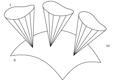
Figure 1. Incomplete Edge as a Cone bundle over $B$.

We call such an edge metric admissible if the fibration $\phi:(\partial M,g_{F}+\phi^{*}g_{B})\to(B,g_{B})$ is a Riemannian submersion. More precisely, we may split the tangent bundle $T_{p}\partial M$ into vertical and horizontal subspaces $T^{V}_{p}\partial M\oplus T^{H}_{p}\partial M$ as follows. The vertical subspace $T^{V}_{p}\partial M$ is the tangent space to the fibre of $\phi$ through $p$, and the horizontal subspace $T^{H}_{p}\partial M$ is the annihilator of the subbundle $T^{V}_{p}\partial M\lrcorner g^{F}\subset T^{*}\partial M$ ($\lrcorner$ denotes contraction). Then $\phi$ is a Riemannian submersion if $g_{F}$ restricted to $T^{H}_{p}\partial M$ vanishes. Any level set $(\{x\}\times\partial M,x^{2}g_{F}+\phi^{*}g_{B})$ is then a Riemannian submersion as well.

Other conditions on the metric $g$ will be added below and are related to the assumption of in a certain sense bounded curvature as well as the spectral analysis of the associated Laplace Beltrami and the Lichnerowicz Laplace operators.

1.2. Geometry of incomplete edge spaces

Choose local coordinates in the singular neighborhood $\mathscr{U}$ as follows. Consider local coordinates $(y)$ on $B$, lifted to $\partial M$ with respect to $\phi$, and then extended radially to $U$. Let coordinates $(z)$ restrict to local coordinates on fibres $F$. This defines local coordinates $(x,y,z)$ in the neighborhood $\mathscr{U}$.

Consider the Lie algebra of edge vector fields $\mathcal{V}_{e}$, which by definition are smooth over $\overline{M}$ and at the boundary $\partial M$ tangent to the fibres of the fibration. In local coordinates, $\mathcal{V}_{e}$ is locally generated by (we write $b:=\dim B$ and $f:=\dim F$)

$$\left\{x\frac{\partial}{\partial x},x\partial_{y}=\left(x\frac{\partial}{\partial y_{1}},\dots,x\frac{\partial}{\partial y_{b}}\right),\partial_{z}=\left(\frac{\partial}{\partial z_{1}},\dots,\frac{\partial}{\partial z_{f}}\right)\right\},$$

with coefficients in the linear combinations of the derivatives being by definition smooth on $\overline{M}$. The vector bundle ${}^{e}TM$ over $\overline{M}$ is defined by requiring that the edge vector fields $\mathcal{V}_{e}$ form a spanning set of sections $\mathcal{V}_{e}=C^{\infty}(\overline{M},{}^{e}TM)$. The dual vector bundle of ${}^{e}TM$ is denoted by ${}^{e}T^{*}M$ and is generated locally by the following one-forms

$$\left\{\frac{dx}{x},\frac{dy_{1}}{x},\dots,\frac{dy_{b}}{x},dz_{1},\dots,dz_{f}\right\}.$$ (1.2)

These differential one-forms, though singular in the usual sense, are smooth as sections of ${}^{e}T^{*}M$. We extend the radial function $x:\mathscr{U}\to(0,1)$ smoothly to $x\in C^{\infty}(\overline{M},[0,\infty))$ such that $x^{-1}(\{0\})=\partial M$ and $dx\restriction\partial M\neq 0$. We define the vector bundle ${}^{ie}TM$ by asking $xC^{\infty}(\overline{M},{}^{ie}TM)=C^{\infty}(\overline{M},{}^{e}TM)$. Its dual, the vector bundle ${}^{ie}T^{*}M$, is related to ${}^{e}T^{*}M$ by $C^{\infty}(\overline{M},{}^{ie}T^{*}M)=xC^{\infty}(\overline{M},{}^{e}T^{*}M)$, and is spanned locally by

$$\left\{dx,dy_{1},\dots,dy_{b},xdz_{1},\dots,xdz_{f}\right\}.$$ (1.3)

Construction of these vector bundles does not require a choice of a Riemannian metric on $M$. Rather the vector bundles ${}^{ie}T^{*}M$ and ${}^{ie}T^{*}M$ allow us to express the structure of the complete edge metric $x^{-2}g$ and the incomplete edge metric $g$, as well as the corresponding curvatures in a convenient way.

The complete edge metric $x^{-2}g$ can be viewed as a smooth section of the symmetric $2$-tensors on ${}^{e}T^{*}M$, which we write as $x^{-2}g\in\textup{Sym}^{2}({}^{e}T^{*}M)$. Therefore we refer to ${}^{e}TM$ and ${}^{e}T^{*}M$ as the complete tangent and cotangent bundles, respectively.

The incomplete edge metric $g$ can be viewed as a smooth section of the symmetric $2$-tensors on ${}^{ie}T^{*}M$, which we write as $g\in\textup{Sym}^{2}({}^{ie}T^{*}M)$. Therefore we refer to ${}^{ie}TM$ and ${}^{ie}T^{*}M$ as the incomplete tangent and cotangent bundles, respectively. We adopt such a convention of incomplete Riemannian edge metrics viewed as sections of $\textup{Sym}^{2}({}^{ie}T^{*}M)$ from now whenever we don’t say otherwise. Note also that the generators of ${}^{ie}TM$ and ${}^{ie}T^{*}M$ are of bounded length with respect to the Riemannian metric $g$ and its inverse, respectively.

The Riemannian curvature $(0,4)$ tensor $R(g)$ acting on $X_{1},X_{2},X_{3},X_{4}\in C^{\infty}(\overline{M},{}^{ie}TM)$ is generically $R(g)[X_{1},X_{2},X_{3},X_{4}]\in x^{-2}C^{\infty}(\overline{M})\equiv\{x^{-2}\cdot u\mid u\in C^{\infty}(\overline{M})\}$. We say in short that $R(g)$ acting on ${}^{ie}TM$ is generically of order $O(x^{-2})$ as $x\to 0$. Similarly, the Ricci curvature tensor $\textup{Ric}(g)$ acting on ${}^{ie}TM$, as well as the scalar curvature $\textup{scal}(g)$, are generically of order $O(x^{-2})$ as $x\to 0$. However, there are geometrically interesting situations, where the Ricci curvature tensor on ${}^{ie}TM$ is bounded up to $x=0$.

First of all, there is of course the example of a flat cone over $\mathbb{S}^{f}$. A second less trivial example is the case of a codimension two singularity, where the normal bundle $NB$ of $B$ inside $TM$ is a fibre bundle over $B$ with the fibre being a two-dimensional disc $\mathbb{D}^{2}$. The involution on $\mathbb{D}^{2}$ defines a global action $\sigma$ on the normal bundle $NB$, which may now be viewed as a branched covering of itself. Any $\sigma$-invariant smooth metric on $NB$ descends to a singular edge metric on $NB/_{\sigma}$ and extends smoothly to $M$. This defines an orbifold metric with incomplete edge singularity and bounded geometry. In a more general setting, any singularity covered by a smooth branched covering space admits a singular metric of bounded Ricci curvature.

The previous paragraph provides two explicit examples of spaces, which have bounded Ricci curvature despite having isolated conical or edge singularities. In both cases the singularity arises as an orbifold singularity. Another class of examples for singular spaces with bounded Ricci curvature has been provided by Hein and Sun [HeSu16], who constructed the first examples of compact Ricci flat manifolds with non-orbifold isolated conical singularities.

Another quite explicit example is the case of a knot $\mathbb{S}^{1}$ embedded into $\mathbb{S}^{3}$ or any other orientable $3$-manifold. The normal bundle of $\mathbb{S}^{1}$ may be equipped with an edge metric of any given angle. The fibres of the normal bundle are flat two-dimensional cones and the resulting metric, smoothly extended away from the singularity, is of bounded geometry.

Let us point out the assumption of a bounded geometry is obviously satisfied in the geometric setting of $g\!\!\mid_{\mathscr{U}}$ being a higher order perturbation of a Ricci-flat incomplete edge metric.

1.3. Hölder spaces on singular manifolds

Definition 1.2.

The Hölder space $\operatorname{\mathcal{C}^{\mathrm{\alpha}}_{\textup{ie}}}(M\times[0,T]),\mathrm{\alpha}\in(0,1),$ consists of functions $u(p,t)$ that are continuous on $\overline{M}\times[0,T]$ with finite $\mathrm{\alpha}$-th Hölder norm

$$\|u\|_{\mathrm{\alpha}}:=\|u\|_{\infty}+\sup\left(\frac{|u(p,t)-u(p^{\prime},t^{\prime})|}{d_{M}(p,p^{\prime})^{\mathrm{\alpha}}+|t-t^{\prime}|^{\frac{\mathrm{\alpha}}{2}}}\right)<\infty,$$ (1.4)

where the distance function $d_{M}(p,p^{\prime})$ between any two points $p,p^{\prime}\in M$ is defined with respect to the incomplete edge metric $g$, and in terms of the local coordinates $(x,y,z)$ in the singular neighborhood $\mathscr{U}$ given equivalently by

$$d_{M}((x,y,z),(x^{\prime},y^{\prime},z^{\prime}))=\left(|x-x^{\prime}|^{2}+(x+x^{\prime})^{2}|z-z^{\prime}|^{2}+|y-y^{\prime}|^{2}\right)^{\frac{1}{2}}.$$

The supremum is taken over all $(p,p^{\prime},t)\in M^{2}\times[0,T]$. We also introduce the Hölder space of time-independent functions (and suppress $[0,T]$ in the notation)

$$\operatorname{\mathcal{C}^{\mathrm{\alpha}}_{\textup{ie}}}(M):=\{u\in\operatorname{\mathcal{C}^{\mathrm{\alpha}}_{\textup{ie}}}(M\times[0,T])\mid u(\cdot,t)\ \textup{is independent of}\ t\in[0,T]\}.$$ (1.5)

We wish to explain in what way the Hölder space $\operatorname{\mathcal{C}^{\mathrm{\alpha}}_{\textup{ie}}}$ introduced above, may be defined locally. Consider any finite cover $\{U_{i}\}_{i\in I}$ of $\overline{M}$ by open coordinate charts and a partition of unity $\{\phi_{j}\}_{j\in J}$ subordinate to that cover. We can define a Hölder norm by

$$\|u\|^{\phi}_{\mathrm{\alpha}}:=\sum_{j\in J}\|\phi_{j}u\|_{\mathrm{\alpha}}.$$ (1.6)

Such a norm is equivalent to our original Hölder norm, since for any tuple $(p,p^{\prime})\in M^{2}$ with distance $d_{M}(p,p^{\prime})>\delta$ bounded away from zero, the quotient in the second summand of the formula (1.4) is bounded by $2\delta^{-1}\|u\|_{\infty}$. Consequently, we may assume without loss of generality that the tuples $(p,p^{\prime})\in M^{2}$ are always taken from within the same coordinate patch of a given atlas.

We also need a notion of Hölder spaces with values in the vector bundle $S=\textup{Sym}^{2}({}^{ie}T^{*}M)$ of symmetric $2$-tensors. with a fibrewise inner product $g_{S}$, induced by the Riemannian metric $g$.

Definition 1.3.

Denote by $h$ a fibrewise inner product on $S=\textup{Sym}^{2}({}^{ie}T^{*}M)$ induced by the Riemannian metric $g$. The Hölder space $\operatorname{\mathcal{C}^{\mathrm{\alpha}}_{\textup{ie}}}(M\times[0,T],S)$ consists of all sections $\mathrm{\omega}$ of $S$ which are continuous on $\overline{M}\times[0,T]$, such that for any local orthonormal frame $\{s_{j}\}$ of $S$, the scalar functions $g_{S}(\mathrm{\omega},s_{j})$ are $\operatorname{\mathcal{C}^{\mathrm{\alpha}}_{\textup{ie}}}(M\times[0,T])$.

The $\mathrm{\alpha}$-th Hölder norm of $\mathrm{\omega}$ is defined using a partition of unity $\{\phi_{j}\}_{j\in J}$ subordinate to a cover of local trivializations of $S$, with a local orthonormal frame $\{s_{jk}\}$ over $\operatorname{supp}(\phi_{j})$ for each $j\in J$. We put

$$\|\mathrm{\omega}\|^{(\phi,s)}_{\mathrm{\alpha}}:=\sum_{j\in J}\sum_{k}\|g_{S}(\phi_{j}\mathrm{\omega},s_{jk})\|_{\mathrm{\alpha}}.$$ (1.7)

As before in (1.6), norms corresponding to different choices of $(\{\phi_{j}\},\{s_{jk}\})$ are equivalent and we may drop the upper index $(\phi,s)$ from notation. The supremum norm $\|\mathrm{\omega}\|_{\infty}$ is defined similarly.

We now define the weighted and higher order Hölder spaces.

Definition 1.4.

1. The weighted Hölder space for $\gamma\in\mathbb{R}$ is

   $$x^{\gamma}\operatorname{\mathcal{C}^{\mathrm{\alpha}}_{\textup{ie}}}(M\times[0,T],S):=\{\,x^{\gamma}\mathrm{\omega}\mid\mathrm{\omega}\in\operatorname{\mathcal{C}^{\mathrm{\alpha}}_{\textup{ie}}}(M\times[0,T],S)\,\},$$

   $$\textup{with H\"{o}lder norm}\ \|x^{\gamma}\mathrm{\omega}\|_{\mathrm{\alpha},\gamma}:=\|\mathrm{\omega}\|_{\mathrm{\alpha}}.$$

2. The hybrid weighted Hölder space for $\gamma\in\mathbb{R}$ is

   $$\operatorname{\mathcal{C}^{\mathrm{\alpha}}_{\textup{ie}}}_{,\gamma}(M\times[0,T],S):=x^{\gamma}\operatorname{\mathcal{C}^{\mathrm{\alpha}}_{\textup{ie}}}(M\times[0,T],S)\,\cap\,x^{\gamma+\mathrm{\alpha}}\mathcal{C}^{0}_{\textup{ie}}(M\times[0,T],S)$$

   $$\textup{with H\"{o}lder norm}\ \|\mathrm{\omega}\|^{\prime}_{\mathrm{\alpha},\gamma}:=\|x^{-\gamma}\mathrm{\omega}\|_{\mathrm{\alpha}}+\|x^{-\gamma-\mathrm{\alpha}}\mathrm{\omega}\|_{\infty}.$$

3. Let $C^{k}(M\times[0,T],S)$ denote the space of $S$-sections that are $k$-times continuously differentiable in the open interior $M$ of $\overline{M}$. We identify the local expressions $\{x\partial_{x},x\partial_{y},\partial_{z}\}$ over $\mathscr{U}$ with their smooth extensions to vector fields over $M$. Then the weighted Hölder spaces of order $k\in\mathbb{N}$ are defined for any weight $\gamma\in\mathbb{R}$ as subspaces of

   $$\begin{split}&\operatorname{\mathcal{C}^{k,\mathrm{\alpha}}_{\textup{ie}}}(M\times[0,T],S)_{\gamma}=\{\mathrm{\omega}\in\operatorname{\mathcal{C}^{\mathrm{\alpha}}_{\textup{ie}}}_{,\gamma}\cap C^{k}\mid\{\operatorname{\mathcal{V}_{e}}^{j}\circ\,(x^{2}\partial_{t})^{\ell}\}\,\mathrm{\omega}\in\operatorname{\mathcal{C}^{\mathrm{\alpha}}_{\textup{ie}}}_{,\gamma}\ \textup{for any}\ j+2\ell\leq k\},\\ &\operatorname{\mathcal{C}^{k,\mathrm{\alpha}}_{\textup{ie}}}(M\times[0,T],S)^{b}_{\gamma}=\{u\in\operatorname{\mathcal{C}^{\mathrm{\alpha}}_{\textup{ie}}}\cap C^{k}\mid\{\operatorname{\mathcal{V}_{e}}^{j}\circ\,(x^{2}\partial_{t})^{\ell}\}\,u\in x^{\gamma}\operatorname{\mathcal{C}^{\mathrm{\alpha}}_{\textup{ie}}}\ \textup{for any}\ j+2\ell\leq k,\\ &\textup{if there is at least one $(x\partial_{x})$ or $\partial_{z}$ derivative included in $\operatorname{\mathcal{V}_{e}}^{j}\circ\,(x^{2}\partial_{t})^{\ell}$},\\ &\textup{otherwise $\operatorname{\mathcal{V}_{e}}^{j}\circ\,(x^{2}\partial_{t})^{\ell}u=(x\partial_{y})^{j}\circ(x^{2}\partial_{t})^{\ell}u\in x^{\min\{\gamma,j+2\ell\}}\operatorname{\mathcal{C}^{\mathrm{\alpha}}_{\textup{ie}}}$}\,\},\end{split}$$

4. In case of $\gamma=0$ we just write $\operatorname{\mathcal{C}^{k,\mathrm{\alpha}}_{\textup{ie}}}=\operatorname{\mathcal{C}^{k,\mathrm{\alpha}}_{\textup{ie}}}(M\times[0,T],S)^{b}_{0}$.

5. The weighted Hölder spaces of time-independent functions are given by

   $$\operatorname{\mathcal{C}^{k,\mathrm{\alpha}}_{\textup{ie}}}(M,S)_{\gamma}:=\{u\in\operatorname{\mathcal{C}^{k,\mathrm{\alpha}}_{\textup{ie}}}(M\times[0,T],S)_{\gamma}\mid u(\cdot,t)\ \textup{is independent of}\ t\in[0,T]\},$$

   $$\operatorname{\mathcal{C}^{k,\mathrm{\alpha}}_{\textup{ie}}}(M,S)^{b}_{\gamma}:=\{u\in\operatorname{\mathcal{C}^{k,\mathrm{\alpha}}_{\textup{ie}}}(M\times[0,T],S)^{b}_{\gamma}\mid u(\cdot,t)\ \textup{is independent of}\ t\in[0,T]\}.$$

In order to define the Hölder norms for $\operatorname{\mathcal{C}^{k,\mathrm{\alpha}}_{\textup{ie}}}(M\times[0,T],S)_{\gamma}$ and $\operatorname{\mathcal{C}^{k,\mathrm{\alpha}}_{\textup{ie}}}(M\times[0,T],S)^{b}_{\gamma}$, we consider as before any finite cover $\{U_{i}\}_{i\in I}$ of $\overline{M}$ by open coordinate charts, which we may assume to trivialize $S$ by appropriate refinement, and a partition of unity $\{\phi_{j}\}_{j\in J}$ subordinate to that cover. By a small abuse of notation we now identify $\mathcal{V}_{e}$ with a finite set of generating edge vector fields, when applied to sections with compact support in $\mathscr{U}$; and write $\mathcal{V}_{e}$ for any local orthonormal frame of vector fields, when applied to sections with compact support in a coordinate chart with distance bounded from below away from the edge singularity. We may now introduce $\mathscr{D}:=\{\operatorname{\mathcal{V}_{e}}^{j}\circ\,(x^{2}\partial_{t})^{\ell}\mid j+2\ell\leq k\}$ and can now write the Hölder norms on the higher order Hölder spaces as follows

$$\begin{split}&\|\mathrm{\omega}\|_{k+\mathrm{\alpha},\gamma}=\sum_{j\in J}\sum_{X\in\mathscr{D}}\|X(\phi_{j}\mathrm{\omega})\|^{\prime}_{\mathrm{\alpha},\gamma}+\|\mathrm{\omega}\|^{\prime}_{\mathrm{\alpha},\gamma},\quad\textup{on}\ \operatorname{\mathcal{C}^{k,\mathrm{\alpha}}_{\textup{ie}}}(M\times[0,T],S)_{\gamma},\\ &\|\mathrm{\omega}\|_{k+\mathrm{\alpha},\gamma}=\sum_{j\in J}\sum_{X\in\mathscr{D}}\|X(\phi_{j}\mathrm{\omega})\|_{\mathrm{\alpha},\gamma}+\|\mathrm{\omega}\|_{\mathrm{\alpha}},\quad\textup{on}\ \operatorname{\mathcal{C}^{k,\mathrm{\alpha}}_{\textup{ie}}}(M\times[0,T],S)^{b}_{\gamma},\end{split}$$ (1.8)

where in the second definition we replace $\|X(\phi_{j}\mathrm{\omega})\|^{\prime}_{\mathrm{\alpha},\gamma}$ by $\|X(\phi_{j}\mathrm{\omega})\|^{\prime}_{\mathrm{\alpha},\min\{\gamma,j+2\ell\}}$ if $X=(x\partial_{y})^{j}\circ(x^{2}\partial_{t})^{\ell}$. Any different choice of coordinate charts and the subordinate partition of unity, as well as different choices of generating vector fields $\mathcal{V}_{e}$ define equivalent Hölder norms.

For sections $\mathrm{\omega}$ compactly supported away from $\partial\overline{M}$, the Hölder norms above are equivalent to the classical parabolic Hölder norms introduced by Ladyzhenskaya, Solonnikov and Ural’tseva [LSU68].

The vector bundle $S$ decomposes into a direct sum of sub-bundles

$$S=S_{0}\oplus S_{1},$$ (1.9)

where the sub-bundle $S_{0}=\textup{Sym}_{0}^{2}({}^{ie}T^{*}M)$ is the space of trace-free (with respect to the fixed metric $g$) symmetric $2$-tensors, and $S_{1}$ is the space of pure trace (with respect to the fixed metric $g$) symmetric $2$-tensors. The sub bundle $S_{1}$ is trivial real vector bundle over $M$ of rank 1. Definition 1.4 extends verbatim to sections of $S_{0}$ and $S_{1}$. Since the sub-bundle $S_{1}$ is a trivial rank one real vector bundle, its sections correspond to scalar functions. Hence, we may omit $S_{1}$ from the notation and simply write e.g.

$$\begin{split}&\operatorname{\mathcal{C}^{k,\mathrm{\alpha}}_{\textup{ie}}}(M\times[0,T])_{\gamma}:=\operatorname{\mathcal{C}^{k,\mathrm{\alpha}}_{\textup{ie}}}(M\times[0,T],S_{1})^{b}_{\gamma},\\ &\operatorname{\mathcal{C}^{k,\mathrm{\alpha}}_{\textup{ie}}}(M)_{\gamma}:=\operatorname{\mathcal{C}^{k,\mathrm{\alpha}}_{\textup{ie}}}(M,S_{1})^{b}_{\gamma}.\end{split}$$ (1.10)

The Hölder spaces $\operatorname{\mathcal{C}^{k,\mathrm{\alpha}}_{\textup{ie}}}(M\times[0,T])^{b}_{\gamma}$ and $\operatorname{\mathcal{C}^{k,\mathrm{\alpha}}_{\textup{ie}}}(M\times[0,T],S)_{\gamma}$ are similar but not the same. They are adapted to the mapping properties of the heat operators for the Laplace Beltrami operator $\Delta$ and the Lichnerowicz Laplacian $\Delta_{L}$ with the former satisfying stochastic completeness. We will address the analytic reason for using such spaces in Remark 4.2.

Moreover, we refer the reader to the Appendix 11 for a detailed comparison of the various Hölder spaces on singular incomplete edge manifolds that appear in the literature, foremost the spaces in [JMR11, BaVe14].

We conclude the subsection with a definition of a Hölder regular geometry.

Definition 1.5.

Let $\mathrm{\alpha}\in(0,1),k\in\mathbb{N}_{0}$ and $\gamma>0$. An admissible edge space $(M,g)$ is $(\mathrm{\alpha},\gamma,k)$-Hölder regular if the following two conditions are satisfied

1. For the curvature $(0,4)$ tensor $R(g)$ acting on any sections $X_{1},X_{2},X_{3},X_{4}\in C^{\infty}(\overline{M},{}^{ie}TM)$

   $$R(g)[X_{1},X_{2},X_{3},X_{4}]\in x^{-2}\mathcal{C}^{k,\mathrm{\alpha}}_{\textup{ie}}(M).$$

2. $\textup{scal}(g)\in x^{-2+\gamma}\mathcal{C}^{k,\mathrm{\alpha}}_{\textup{ie}}(M)$ and the trace-free part of $\textup{Ric}(g)$ is $\mathcal{C}^{k,\mathrm{\alpha}}_{\textup{ie}}(M,S_{0})_{-2+\gamma}$.

1.4. Existence of the singular Ricci flow

Given a compact smooth Riemannian manifold $(M,g_{0})$, the Ricci flow of $g_{0}$ is by definition a family $g(t),t\in[0,T]$ of Riemannian metrics on $M$, satisfying the Ricci flow equation

$$\partial_{t}g(t)=-2\,\textup{Ric}(g(t)),\quad g(0)=g_{0}.$$ (1.11)

Ricci flow is not a parabolic equation due to its diffeomorphism invariance. Therefore existence of solutions does not follow directly from the classical parabolic theory. This problem is resolved using the so-called de Turck trick [Tur03]. The de Turck trick leads to an equivalent Ricci de Turck flow $g(t)$, which is given by the following equation.

$$\partial_{t}g(t)=-2\,\textup{Ric}(g(t))+\mathcal{L}_{W(t)}g(t),\quad g(0)=g_{0},$$ (1.12)

where $W(t)$ is the de Turck vector field defined in terms of the Christoffel symbols for the metrics $g(t)$ and a reference metric $\widetilde{g}$

$$W(t)^{k}=g(t)^{ij}\left(\Gamma^{k}_{ij}(g(t))-\Gamma^{k}_{ij}(\widetilde{g})\right).$$ (1.13)

The de Turck vector field $W(t)$ yields a one parameter family of diffeomorphisms $\phi(t)$ and the pullback $\phi(t)^{*}g(t)$ solves the Ricci flow (1.11). Ricci de Turck flow is a parabolic equation and existence of its solution can be easily obtained by the following argument. The equation (1.12) is linearized by writing $g(t)=v(t)+g_{0}$, which leads to a non-linear parabolic equation for $v(t)$

$$(\partial_{t}+\Delta_{L})v(t)=-2\,\textup{Ric}(g_{0})+O_{2}(v(t)),\quad v(0)=0,$$ (1.14)

where $\Delta_{L}$ is the Lichnerowicz Laplacian on symmetric two-tensors and $O_{2}(v(t))$ is a sum of terms which are at least quadratic in $v(t)$ and its first and second order derivatives. Clearly, the solution $v(t)$ is a fixed point of the following map

$$\begin{split}\Phi:&\ C^{2,\alpha}(M\times[0,T])\longrightarrow C^{2,\alpha}(M\times[0,T]),\\ &u\mapsto\int_{0}^{t}e^{-(t-\widetilde{t})\,\Delta_{L}}\left(-2\,\textup{Ric}(g_{0})+O_{2}(u(\widetilde{t}))\right)d\widetilde{t},\end{split}$$ (1.15)

where $e^{-t\,\Delta_{L}}$ is the heat operator of the Lichnerowicz Laplacian $\Delta_{L}$ and $C^{k,\alpha}$ are the usual parabolic Hölder spaces with $\alpha\in(0,1)$ and $k\in\mathbb{N}_{0}$. Classical Schauder estimates of Ladyzhenskaya, Solonnikov and Ural’tseva [LSU68] essentially prove the mapping property of the heat operator (acting with a convolution in time)

$$\begin{split}e^{-t\,\Delta_{L}}:&\ C^{0,\alpha}(M\times[0,T])\longrightarrow C^{2,\alpha}(M\times[0,T]),\\ &u\mapsto\int_{0}^{t}e^{-(t-\widetilde{t})\,\Delta_{L}}u(\widetilde{t})d\widetilde{t},\end{split}$$ (1.16)

and imply that $\Phi$ is bounded, since $O_{2}(u(\widetilde{t}))\in C^{0,\alpha}$ for $u\in C^{2,\alpha}$. A simple argument shows that for $\mu>0$ sufficiently small, $\Phi$ is a contraction on

$$Z_{\mu,T}:=\{u\in C^{2,\alpha}(M\times[0,T])\mid\|u\|_{2,\mathrm{\alpha}}\leq\mu\},$$ (1.17)

mapping $Z_{\mu,T}$ to itself for $\mu,T>0$ sufficiently small. Consequently, by the Banach fixed point theorem there exists a fixed point $v(t)$ of $\Phi$, which is a solution to the Ricci de Turck flow by construction.

While on smooth compact manifolds, Ricci flow continues to be a focal point of intensive research, on singular spaces even existence of Ricci flow is an open problem. If the manifold $(M.g)$ is singular, the argument outlined above may break down. The major difficulty hereby is whether some analogue of parabolic Schauder estimates as derived in [LSU68] can be established in the singular setting. The purpose of the present work is to study the Ricci de Turck flow on a singular edge manifolds. We derive parabolic Schauder estimates in this setting and prove short time existence of Ricci de Turck flow.

Our first main result establishes short time existence of Ricci de Turck flow starting at an admissible incomplete edge metric of Hölder regular geometry and flowing through the space of singular metrics, which preserves the admissible edge structure and Hölder regular geometry. The result holds under an additional assumption of tangential stability, which is a spectral condition imposed upon the Lichnerowicz Laplace operator introduced below in Definition 2.1 and discussed in detail in Theorem 2.2. Let us point out that [KrVe17, Theorem 1.4] provides an extensive list of explicit examples, where tangential stability is satisfied.

Theorem 1.6.

Consider an incomplete edge manifold $(M,g)$ with an admissible edge metric and Hölder-regular geometry, satisfying the assumption of tangential stability. Then for short time $g$ may be evolved under the Ricci de Turck flow into a family of Riemannian metrics $g(t)$ within the space of admissible edge metrics of Hölder regular geometry for some finite time $T>0$.

We will also address the relation between the Ricci de Turck and the Ricci flow, which is intricate in terms of regularity.

Our second main result concerns Ricci flow starting at metrics that are in a certain sense higher order small perturbations of flat incomplete edge metrics. In that case we actually obtain long time existence.

Theorem 1.7.

Consider an incomplete edge manifold $(M,h)$ of Hölder regular geometry with an admissible flat edge metric, satisfying the assumption of tangential stability. If $g_{0}$ is a higher order sufficiently small perturbation of $h$, then a Ricci de Turck flow $g(t)$ of admissible incomplete edge metrics of Hölder regular geometry, starting at $g_{0}$, exists for all time and stays in a small $\varepsilon$-neighborhood of $h$, uniformly in $t\geq 0$.

In a joint paper with Kröncke [KrVe17] we discuss stability of the Ricci de Turck flow for small perturbations of Ricci flat (not necessarily flat) singular metrics, assuming certain integrability conditions outside of the scope of the present paper.

In fact, Ricci flow through singular metrics has been studied by various authors in dimension two, e.g. by Mazzeo, Rubinstein and Sesum in [MRS11], our work jointly with Bahuaud in [BaVe14]. Somewhat different from the approach taken here, is the work by Giesen and Topping on instantaneously complete Ricci flow in [GiTo10] and [GiTo11]. Another alternative approach has been taken by Miles Simon in [Sim13], where Ricci flow smoothens out any Lipschitz singularity instantly.

The idea of the proof for both Theorem 1.6 and Theorem 1.7 is, exactly as in the compact smooth case, to linearize the Ricci de Turck flow and apply Banach fixed point theorem in appropriate Hölder spaces. This requires mapping properties of the heat operator for the Lichnerowicz Laplacian. The bulk of the paper is therefore devoted to deriving these mapping properties in the singular setting.

This paper is organized as follows. We begin with the analysis of the Lichnerowicz Laplace operator in §2 and construct a solution to its heat equation as a polyhomogeneous conormal distribution on a blown up heat space. In §4 we establish various mapping properties of the heat operator for the Lichnerowicz and the Laplace Beltrami operators. We employ these mapping properties to establish existence of a solution to the Ricci de Turck flow in §5 and show in §6 that this flow is indeed a flow of admissible incomplete edge metrics. Then §7 explains how to pass from the Ricci de Turck solution to the corresponding solution of the Ricci flow, along with a change in regularity. In §8 we discuss Hölder regularity of the Ricci de Turck flow for positive times, an aspect which will be crucial in subsequent maximum principle arguments. We conclude this paper with a long time existence result in §9 for Ricci flow of metrics that are sufficiently small perturbations of flat edge metrics.

Acknowledgements: The author thanks Burkhard Wilking, Christoph Böhm, Rafe Mazzeo and Eric Bahuaud for important discussions about aspects of Ricci flow and encouragement. He thanks Klaus Kröncke for helpful discussions concerning computations in his paper on Einstein warped products. He is grateful to the anonymous referee for careful reading of the manuscript, important remarks and suggestions. The author also gratefully acknowledges support of the Mathematical Institute at Münster University.

2. Lichnerowicz Laplacian on $2$-tensors of an exact cone

In this section we study the rough and the Lichnerowicz Laplace operators acting on symmetric $2$-tensors over an exact cone $\mathscr{C}(F):=(0,1)\times F$ with an exact conical metric $g=dx^{2}\oplus x^{2}g_{F}$. We provide explicit formulae and formulate assumptions that are necessary for the subsequent analytic arguments.

Consider for the moment any Riemannian manifold $(M,g)$ of dimension $m$. We will specify $M$ to be an exact cone $\mathscr{C}(F)$ right after the general definition. Let $L$ denote any vector bundle associated to $T^{*}M$, for instance the bundle $S$ of symmetric trace-free $2$-tensors $\textup{Sym}^{2}_{0}(T^{*}M)$. Let $\nabla$ denote the induced Levi-Civita connection acting on smooth compactly supported sections as

$$\nabla:C^{\infty}_{0}(M,L)\to C^{\infty}_{0}(M,L\otimes T^{*}M),$$

$$\nabla^{2}:C^{\infty}_{0}(M,L)\to C^{\infty}_{0}(M,L\otimes T^{*}M\otimes T^{*}M).$$

The rough Laplacian $\Delta$, acting on smooth compactly supported sections of $L$, is then defined as follows. Consider the pointwise inner product on fibres of $L$, induced by the Riemannian metric $g$ on $M$. Let $\{e_{i}\}_{i=1}^{m}$ denote a local orthonormal frame of $TM$, where $m$ is the dimension of $M$. The rough Laplacian is given by

$$\Delta:=-\sum_{i=1}^{m}\nabla^{2}_{e_{i}e_{i}}\equiv-\textup{tr}(\nabla^{2}).$$ (2.1)

The Lichnerowicz Laplacian on symmetric covariant $2$-tensors is defined in terms of the rough Laplacian $\Delta$ and additional curvature terms by

$$\Delta_{L}:=\Delta+2(\textup{Ric}-\textup{Riem}),$$ (2.2)

where for any symmetric covariant $2$-tensor $\mathrm{\omega}$ on any Riemannian manifold $(M,g)$, with the corresponding curvature tensor $\textup{Riem}(g)$ and the Ricci curvature tensor $\textup{Ric}(g)$, we have

$$\begin{split}&(\textup{Ric}\,\mathrm{\omega})_{ij}:=\left(\textup{Ric}(g)_{ik}\,g^{k\ell}\mathrm{\omega}_{\ell j}+\textup{Ric}(g)_{jk}\,g^{k\ell}\mathrm{\omega}_{\ell i}\right)/2,\\ &(\textup{Riem}\,\mathrm{\omega})_{ij}:=\textup{Riem}(g)_{ikj\ell}\,g^{ks}g^{\ell t}\mathrm{\omega}_{st}.\end{split}$$ (2.3)

Let us now specify the action of $\Delta_{L}$ in case of an exact cone. Let $M=\mathscr{C}(F):=(0,1)\times F$ be an exact cone with an exact conical metric $g=dx^{2}\oplus x^{2}g_{F}$. Let $L=\textup{Sym}^{2}({}^{ie}T^{*}\mathscr{C}(F))$ be the bundle of symmetric covariant $2$-tensors on the cone. We may decompose

$$C^{\infty}_{0}(\mathscr{C}(F),L)\equiv C^{\infty}_{0}(\mathscr{C}(F),\textup{Sym}^{2}({}^{ie}T^{*}\mathscr{C}(F)))=C^{\infty}_{0}(\mathscr{C}(F))g\oplus C^{\infty}_{0}(\mathscr{C}(F),S_{0})$$

into the pure trace and the trace-free parts with respect to the Riemannian edge metric $g$. This decomposition is preserved under the Lichnerowicz Laplacian. By a minor abuse of notation, $\Delta_{L}$ shall refer to the Lichnerowicz Laplacian on the trace-free part, while $\Delta^{\prime}_{L}$ denotes its action on the pure trace component. $\Delta^{\prime}_{L}$ is given by the action of the Laplace Beltrami operator with ($f=\dim F$)

$$\Delta^{\prime}_{L}(u\cdot g)=\left(-\partial_{x}^{2}u-\frac{f}{x}\partial_{x}u+\frac{1}{x^{2}}\,\square^{\prime}_{L}u\right)\cdot g,$$ (2.4)

where $\square^{\prime}_{L}$ is the Laplace Beltrami operator of $(F,g_{F})$. The action of $\Delta_{L}$ on the trace-free component has been computed by Delay [Del06, Lemma 4.2] and Guillarmou, Moroianu and Schlenker [GMS12, 7.4]. Let $\{z_{\alpha}\}$ denote local coordinates on $F$. We write for any symmetric trace-free $2$-tensor $\mathrm{\omega}\in C^{\infty}_{0}(\mathscr{C}(F),S_{0})$

$$\mathrm{\omega}_{xx}:=\mathrm{\omega}(\partial_{x},\partial_{x}),\quad \mathrm{\omega}_{x\mathrm{\alpha}}:=\mathrm{\omega}(\partial_{x},x^{-1}\partial_{z_{\mathrm{\alpha}}}),\qquad\mathrm{\omega}_{\mathrm{\alpha}\beta}:=\mathrm{\omega}(x^{-1}\partial_{z_{\mathrm{\alpha}}},x^{-1}\partial_{z_{\beta}});$$

$$\mathrm{\omega}^{\prime}_{x\mathrm{\alpha}}:=\mathrm{\omega}(\partial_{x},\partial_{z_{\mathrm{\alpha}}})=x\,\mathrm{\omega}_{x\mathrm{\alpha}},\quad\mathrm{\omega}^{\prime}_{\mathrm{\alpha}\beta}:=\mathrm{\omega}(\partial_{z_{\mathrm{\alpha}}},\partial_{z_{\beta}})=x^{2}\mathrm{\omega}_{\mathrm{\alpha}\beta}.$$

For simplicity of notation we denote the scalar function $\mathrm{\omega}_{xx}$ by $\eta$, the $(1,0)$-tensor $(\mathrm{\omega}^{\prime}_{x\mathrm{\alpha}})_{\mathrm{\alpha}}$ by $\xi^{\prime}$, and the symmetric $2$-tensor $(\mathrm{\omega}^{\prime}_{\mathrm{\alpha}\beta})_{\mathrm{\alpha}\beta}$ on the cross section of the cone by $\kappa^{\prime}$. Clearly, our convention is to use greek letters for components corresponding to the cross section $F$. Operators and quantities referring to the cross section $(F,g_{F})$ of the cone $\mathscr{C}(F)$ are denoted with an additional index $F$. Then we obtain as in [Del06, Lemma 4.2] and [GMS12, 7.4]

$$(\Delta_{L}\mathrm{\omega})_{xx}=\left(-\partial_{x}^{2}-\frac{f}{x}\partial_{x}+\frac{1}{x^{2}}\left(\Delta^{F}_{L}+2f+2\right)\right)\eta-\frac{4}{x^{3}}\delta_{F}\xi^{\prime},$$

$$(\Delta_{L}\mathrm{\omega})^{\prime}_{x\mathrm{\alpha}}=\left(-\partial_{x}^{2}-\frac{f-2}{x}\partial_{x}+\frac{1}{x^{2}}\left(\Delta^{F}_{L}+f+2\right)\right)\xi^{\prime}_{\mathrm{\alpha}}-\frac{2}{x}\partial_{z_{\mathrm{\alpha}}}\eta+\frac{2}{x^{3}}\delta_{F}\kappa^{\prime}_{\mathrm{\alpha}},$$

$$(\Delta_{L}\mathrm{\omega})^{\prime}_{\mathrm{\alpha}\beta}=\left(-\partial_{x}^{2}-\frac{f-4}{x}\partial_{x}+\frac{1}{x^{2}}\left(\Delta^{F}_{L}-4\right)\right)\kappa^{\prime}_{\mathrm{\alpha}\beta}-2\,\eta\,g^{F}_{\mathrm{\alpha}\beta}$$

$$\qquad\qquad\qquad\qquad\qquad\qquad\qquad\qquad+\frac{2}{x^{2}}(\textup{tr}_{g_{F}}\kappa^{\prime})g^{F}_{\mathrm{\alpha}\beta}-\frac{2}{x}\delta^{*}_{F}\xi^{\prime}_{\mathrm{\alpha}\beta},$$

where $\Delta^{F}_{L}$ acting on $h$ refers to the Lichnerowicz Laplacian acting on symmetric $2$-forms over $F$ and moreover, we have introduced the following notation

$$\Delta^{F}_{L}\eta:=\Delta_{F}\eta\equiv\square^{\prime}_{L}\eta,\quad\delta_{F}\xi^{\prime}:=g_{F}^{\mathrm{\alpha}\beta}(\nabla^{F}_{\beta}\xi^{\prime})_{\mathrm{\alpha}},$$

$$\Delta^{F}_{L}\xi^{\prime}_{\mathrm{\alpha}}:=(\nabla_{F}^{*}\nabla_{F}\xi^{\prime})_{\mathrm{\alpha}}+g_{F}^{\gamma\beta}\textup{Ric}^{F}_{\beta\mathrm{\alpha}}\xi^{\prime}_{\gamma},\quad\delta_{F}\kappa^{\prime}_{\mathrm{\alpha}}:=g_{F}^{\gamma\beta}(\nabla^{F}_{\beta}\kappa^{\prime})_{\mathrm{\alpha}\gamma},$$

$$(\delta^{*}_{F}\xi^{\prime})_{\mathrm{\alpha}\beta}:=(\nabla^{F}_{\mathrm{\alpha}}\xi^{\prime})_{\beta}+(\nabla^{F}_{\beta}\xi^{\prime})_{\mathrm{\alpha}}.$$

The formulae become more transparent if we switch to the action on $(\mathrm{\omega}_{xx},\mathrm{\omega}_{x\mathrm{\alpha}},\mathrm{\omega}_{\mathrm{\alpha}\beta})$. We denote the $(1,0)$-tensor $(\mathrm{\omega}_{x\mathrm{\alpha}})_{\mathrm{\alpha}}$ by $\xi$, and the symmetric $2$-tensor $(\mathrm{\omega}_{\mathrm{\alpha}\beta})_{\mathrm{\alpha}\beta}$ on the cross section of the cone by $\kappa$. Clearly, $\xi^{\prime}=x\xi$ and $\kappa^{\prime}=x^{2}\kappa$. The action of the Lichnerowicz Laplacian with respect to that rescaling is now given by

$$(\Delta_{L}\mathrm{\omega})_{xx}=\left(-\partial_{x}^{2}-\frac{f}{x}\partial_{x}+\frac{1}{x^{2}}\left(\Delta^{F}_{L}+2f+2\right)\right)\eta-\frac{4}{x^{2}}\delta_{N}\xi,$$

$$(\Delta_{L}\mathrm{\omega})_{x\mathrm{\alpha}}=\left(-\partial_{x}^{2}-\frac{f}{x}\partial_{x}+\frac{1}{x^{2}}\left(\Delta^{F}_{L}+4\right)\right)\xi_{\mathrm{\alpha}}-\frac{2}{x^{2}}\partial_{z_{\mathrm{\alpha}}}\eta+\frac{2}{x^{2}}\delta_{F}\kappa_{\mathrm{\alpha}},$$

$$(\Delta_{L}\mathrm{\omega})_{\mathrm{\alpha}\beta}=\left(-\partial_{x}^{2}-\frac{f}{x}\partial_{x}+\frac{1}{x^{2}}\left(\Delta^{F}_{L}+2-2f\right)\right)\kappa_{\mathrm{\alpha}\beta}-\frac{2}{x^{2}}\,\eta\,g^{F}_{\mathrm{\alpha}\beta}$$

$$\qquad\qquad\qquad\qquad\qquad\qquad\qquad\qquad+\frac{2}{x^{2}}(\textup{tr}_{g_{F}}\kappa)g^{F}_{\mathrm{\alpha}\beta}-\frac{2}{x^{2}}\delta^{*}_{F}\xi_{\mathrm{\alpha}\beta},$$

Identifying any trace-free $\mathrm{\omega}$ with the vector of its $(\mathrm{\omega}_{xx},\mathrm{\omega}_{x\mathrm{\alpha}},\mathrm{\omega}_{\mathrm{\alpha}\beta})$ components,

$$\begin{split}C^{\infty}_{0}(\mathscr{C}(F),S_{0})&\to C^{\infty}_{0}((0,1),C^{\infty}(F)\times\Omega^{1}(F)\times\textup{Sym}^{2}(T^{*}F)),\\ \mathrm{\omega}&\mapsto(\mathrm{\omega}_{xx},\mathrm{\omega}_{x\mathrm{\alpha}},\mathrm{\omega}_{\mathrm{\alpha}\beta}),\end{split}$$ (2.5)

where $\Omega^{1}(F)$ denotes differential $1$-forms on $F$, we arrive at the following expression for the action of the Lichnerowicz Laplacian on $\mathrm{\omega}\equiv(\mathrm{\omega}_{xx},\mathrm{\omega}_{x\mathrm{\alpha}},\mathrm{\omega}_{\mathrm{\alpha}\beta})$

$$\Delta_{L}\mathrm{\omega}=\left(-\partial_{x}^{2}-\frac{f}{x}\partial_{x}+\frac{1}{x^{2}}\,\square_{L}\right)\mathrm{\omega},$$ (2.6)

where the action of $\square_{L}$ is given by

$$\square_{L}=\left(\begin{array}[]{clc}\Delta^{F}_{L}+2f+2&-4\delta_{F}&0\\ -2\partial_{z}&\Delta^{F}_{L}+4&2\delta_{F}\\ -2g_{F}&-2\delta_{F}^{*}&\Delta^{F}_{L}+2-2f+2g_{F}\textup{tr}_{g_{F}}\end{array}\right).$$ (2.10)

We may now introduce the assumption of tangential stability.

Definition 2.1.

We call an admissible edge manifold $(M,g)$ tangentially stable with lower bounds $u_{0},u_{1}>0$, if $\min(\textup{Spec}\,\square_{L})=u_{0}$ and $\min(\textup{Spec}\,\square^{\prime}_{L}\backslash\{0\})=u_{1}$.

In the follow-up joint work with Kröncke [KrVe17, Theorem 1.3] we characterize tangential stability explicitly in terms of the spectrum of the Einstein and the Hodge Laplace operators on the cross section $(F,g_{F})$. We state the result here for completeness.

Theorem 2.2.

Let $(F,g_{F})$ be a compact Einstein manifold of dimension $f\geq 3$ with the Einstein constant $(f-1)$. We write $\Delta_{E}$ for its Einstein operator, and denote the Laplace Beltrami operator by $\Delta$. Then tangential stability holds if and only if $\mathrm{Spec}(\Delta_{E}|_{TT})>0$ and $\mathrm{Spec}(\Delta)\setminus\left\{0\right\}\cap(f,2(f+1)]=\varnothing$.

We also identify in [KrVe17, Theorem 1.4] an extensive list of explicit examples, where tangential stability is satisfied. This includes e.g. certain simple Lie groups and rank-1 symmetric spaces of compact type. The actual statement in [KrVe17] also identifies the cases where tangential stability fails. Moreover [KrVe17] shows that the only example where $(F,g_{F})$ is weakly tangentially stable in the sense of Definition 9.1, but not tangentially stable is the case of a sphere.

3. Heat operator of the Lichnerowicz Laplacian

We consider the Lichnerowicz Laplacian $\Delta_{L}$, acting on trace-free symmetric two-tensors on an admissible incomplete edge manifold $(M,g)$. In this subsection we consider the homogeneous or the inhomogeneous heat equations

$$\begin{split}&(\partial_{t}+\Delta_{L})\,\mathrm{\omega}_{\textup{hom}}(t,p)=0,\ \mathrm{\omega}_{\textup{hom}}(0,p)=\mathrm{\omega}_{0}(p),\\ &(\partial_{t}+\Delta_{L})\,\mathrm{\omega}_{\textup{inhom}}(t,p)=v(t,p),\ \mathrm{\omega}_{\textup{inhom}}(0,p)=0,\\ \end{split}$$ (3.1)

and obtain their fundamental solutions, following the heat kernel construction of [MaVe12]. The solutions are given in terms of an integral convolution operator acting on compactly supported sections such that

$$\begin{split}&\mathrm{\omega}_{\textup{hom}}(t,p)=\left(e^{-t\Delta_{L}}\mathrm{\omega}_{0}\right)(t,p):=\int_{M}\left(e^{-t\,\Delta_{L}}\left(p,\widetilde{p}\right),\mathrm{\omega}_{0}(\widetilde{p})\right)_{g}\operatorname{dvol_{g}}(\widetilde{p}),\\ &\mathrm{\omega}_{\textup{inhom}}(t,p)=\left(e^{-t\Delta_{L}}v\right)(t,p):=\int_{0}^{t}\int_{M}\left(e^{-(t-\widetilde{t})\,\Delta_{L}}\left(p,\widetilde{p}\right),v(\widetilde{t},\widetilde{p})\right)_{g}\operatorname{dvol_{g}}(\widetilde{p})d\widetilde{t}.\end{split}$$ (3.2)

In both cases we denote the fundamental solution by $e^{-t\Delta_{L}}$, which acts by time convolution on time-dependent sections.

Under the additional assumption $\Delta_{L}\geq 0$ on smooth compactly supported sections of $S_{0}$, the fundamental solution $e^{-t\Delta_{L}}$ can be identified with the heat operator of the Friedrichs self-adjoint extension of the Lichnerowicz Laplacian. This will be explained below in Theorem 3.5 and is crucial later on for the argument on the long time existence of the Ricci flow starting at small perturbations of flat metrics.

3.1. Heat kernel of a model operator

Before we proceed with an asymptotic analysis of the fundamental solution for the Lichnerowicz Laplacian $\Delta_{L}$ on an admissible edge manifold $(M,g)$, we consider a model operator which already comprises all the central properties of $\Delta_{L}$. Let us write $\mathbb{R}_{+}:=(0,\infty)$. Consider for any $\mu\geq 0$ the model operator

$$\ell_{\mu}:=-\frac{d^{2}}{ds^{2}}-\frac{f}{s}\frac{d}{ds}+\frac{1}{s^{2}}\left(\mu^{2}-\left(\frac{f-1}{2}\right)^{2}\right):C^{\infty}_{0}(\mathbb{R}_{+})\to C^{\infty}_{0}(\mathbb{R}_{+}),$$ (3.3)

acting on compactly supported smooth test functions $C^{\infty}_{0}(\mathbb{R}_{+})$. This operator is symmetric with respect to the inner product of $L^{2}(\mathbb{R}_{+},s^{f}ds)$. It can be conveniently studied under the unitary rescaling transformation $\Phi:L^{2}(\mathbb{R}_{+},s^{f}ds)\to L^{2}(\mathbb{R}_{+},ds)$ with $\Phi(u)=s^{f/2}u$. Then

$$\Phi\circ\ell_{\mu}\circ\Phi^{-1}=-\frac{d^{2}}{ds^{2}}+\frac{1}{s^{2}}\left(\mu^{2}-\frac{1}{4}\right)=:L_{\mu},$$ (3.4)

is a symmetric operator in $L^{2}(\mathbb{R}_{+},ds)$. Consider the maximal and minimal domains for $L_{\mu}$ acting on $C^{\infty}_{0}(\mathbb{R}_{+})$

$$\begin{split}\mathscr{D}_{\max}(L_{\mu}):=\{&\mathrm{\omega}\in L^{2}(\mathbb{R}_{+})\mid L_{\mu}\mathrm{\omega}\in L^{2}(\mathbb{R}_{+})\},\\ \mathscr{D}_{\min}(L_{\mu}):=\{&\mathrm{\omega}\in\mathscr{D}_{\max}(L_{\mu})\mid\exists(\mathrm{\omega}_{n})\subset C^{\infty}_{0}(\mathbb{R}_{+}):\\ &\mathrm{\omega}_{n}\xrightarrow{L^{2}}\mathrm{\omega},\quad L_{\mu}\mathrm{\omega}_{n}\xrightarrow{L^{2}}L_{\mu}\mathrm{\omega}\},\end{split}$$ (3.5)

where $L_{\mu}\mathrm{\omega}\in L^{2}(\mathbb{R}_{+})$ on $\mathrm{\omega}\in L^{2}(\mathbb{R}_{+})$ is understood in the distributional sense. The maximal (minimal) domain of $\ell_{\mu}$ is defined similarly and the domains are related by the unitary transformation $\Phi$

$$\mathscr{D}_{\max}(\ell_{\mu})=\Phi^{-1}\mathscr{D}_{\max}(L_{\mu}),\quad\mathscr{D}_{\min}(\ell_{\mu})=\Phi^{-1}\mathscr{D}_{\min}(L_{\mu}).$$

By explicit computations, see for example [Ver09, Proposition 2.10], any $\mathrm{\omega}\in\mathscr{D}_{\max}(L_{\mu})$ admits an asymptotic expansion

$$\begin{split}&\mathrm{\omega}=c^{+}_{\mu}(\mathrm{\omega})\,x^{\frac{1}{2}}+c^{-}_{\mu}(\mathrm{\omega})\,x^{\frac{1}{2}}\log(x)+\widetilde{\mathrm{\omega}},\quad\textup{if}\ \mu=0,\\ &\mathrm{\omega}=c^{+}_{\mu}(\mathrm{\omega})\,x^{\mu+\frac{1}{2}}+c^{-}_{\mu}(\mathrm{\omega})\,x^{-\mu+\frac{1}{2}}+\widetilde{\mathrm{\omega}},\quad\textup{if}\ \mu\in(0,1),\\ &\mathrm{\omega}=\widetilde{\mathrm{\omega}},\quad\textup{if}\ \mu\geq 1,\\ \end{split}$$ (3.6)

with coefficients $c^{\pm}_{\mu}(\mathrm{\omega})\in\mathbb{C}$ and $\widetilde{\mathrm{\omega}}\in\mathscr{D}_{\min}(L_{\mu})$. Hence any $\mathrm{\omega}\in\mathscr{D}_{\max}(\ell_{\mu})=\Phi^{-1}\mathscr{D}_{\max}(L_{\mu})$ admits an asymptotic expansion

$$\begin{split}&\mathrm{\omega}=c^{+}_{\mu}(\mathrm{\omega})\,x^{-\frac{(f-1)}{2}}+c^{-}_{\mu}(\mathrm{\omega})\,x^{-\frac{(f-1)}{2}}\log(x)+\widetilde{\mathrm{\omega}},\quad\textup{if}\ \mu=0,\\ &\mathrm{\omega}=c^{+}_{\mu}(\mathrm{\omega})\,x^{\mu-\frac{(f-1)}{2}}+c^{-}_{\mu}(\mathrm{\omega})\,x^{-\mu-\frac{(f-1)}{2}}+\widetilde{\mathrm{\omega}},\quad\textup{if}\ \mu\in(0,1),\\ &\mathrm{\omega}=\widetilde{\mathrm{\omega}},\quad\textup{if}\ \mu\geq 1,\\ \end{split}$$ (3.7)

with coefficients $c^{\pm}_{\mu}(\mathrm{\omega})\in\mathbb{C}$ and $\widetilde{\mathrm{\omega}}\in\mathscr{D}_{\min}(\ell_{\mu})$. We set $c^{\pm}_{\mu}(\mathrm{\omega})=0$ for $\mu\geq 1$. For any $\mathrm{\omega},v\in\mathscr{D}_{\max}(\ell_{\mu})$ we compute using integration by parts

$$\begin{split}&\langle L_{\mu}\Phi\mathrm{\omega},\Phi v\rangle_{L^{2}(\mathbb{R}_{+},ds)}-\langle\Phi\mathrm{\omega},L_{\mu}\Phi v\rangle_{L^{2}(\mathbb{R}_{+},ds)}=\\ &\langle\ell_{\mu}\mathrm{\omega},v\rangle_{L^{2}(\mathbb{R}_{+},s^{f}ds)}-\langle\mathrm{\omega},\ell_{\mu}v\rangle_{L^{2}(\mathbb{R}_{+},s^{f}ds)}=c_{\mu}\left(c^{+}_{\mu}(\mathrm{\omega})\overline{c^{-}_{\mu}(v)}-c^{-}_{\mu}(\mathrm{\omega})\overline{c^{+}_{\mu}(v)}\right).\end{split}$$ (3.8)

where $c_{\mu}=-1$ for $\mu=0$ and $c_{\mu}=2\mu$ otherwise. From this formula it becomes clear that boundary conditions need to be imposed on the coefficients $c^{\pm}_{\mu}(\mathrm{\omega})$ in order to obtain a self-adjoint extension of $\ell_{\mu}$ and $L_{\mu}$ In case $\mu\geq 1$, $\ell_{\mu}$ and $L_{\mu}$ are essentially self-adjoint, since no boundary terms appear after integration by parts in (3.8).

Existence of a self-adjoint extension of $L_{\mu}$ and $\ell_{\mu}$ with the same lower bound as $L_{\mu}$ and $\ell_{\mu}$, respectively, both acting on $C^{\infty}_{0}(\mathbb{R}_{+})$, is due to Friedrichs and Stone, see Riesz and Nagy [RiNa90, Theorem on p. 330], who introduced the so-called Friedrichs self-adjoint extension. Providing the functional analytic construction of the Friedrichs extension is out of scope of the present discussion. However the Friedrichs extension $L^{\mathscr{F}}_{\mu}$ of $L_{\mu}$, as well as the Friedrichs extension $\ell^{\mathscr{F}}_{\mu}$ of $\ell_{\mu}$ can be explicitly characterized as follows

$$\begin{split}&\mathscr{D}(L^{\mathscr{F}}_{\mu})=\{\mathrm{\omega}\in\mathscr{D}_{\max}(L_{\mu})\mid c^{-}_{\mu}(\mathrm{\omega})=0\},\\ &\mathscr{D}(\ell^{\mathscr{F}}_{\mu})=\{\mathrm{\omega}\in\mathscr{D}_{\max}(\ell_{\mu})\mid c^{-}_{\mu}(\mathrm{\omega})=0\}.\end{split}$$ (3.9)

Both extensions are related by the unitary transformation

$$L^{\mathscr{F}}_{\mu}=\Phi\circ\ell^{\mathscr{F}}_{\mu}\circ\Phi^{-1},\quad\mathscr{D}(\ell^{\mathscr{F}}_{\mu})=\Phi^{-1}\mathscr{D}(L^{\mathscr{F}}_{\mu}).$$

The heat kernel $H_{\mu}$ of the Friedrichs extension $L^{\mathscr{F}}_{\mu}$ is well-known and [Les97, Proposition 2.3.9] provided its explicit expression in terms of the modified Bessel function $I_{\mu}$ of first kind

$$H_{\mu}(t,s,\widetilde{s})=\frac{1}{2t}(s\widetilde{s})^{1/2}I_{\mu}\left(\frac{s\widetilde{s}}{2t}\right)e^{-\frac{s^{2}+\widetilde{s}^{2}}{4t}}.$$ (3.10)

Hence, the heat kernel $e^{-t\ell_{\mu}}$ of $\ell^{\mathscr{F}}_{\mu}$ is given by $(s\widetilde{s})^{-f/2}H_{\mu}(t,s,\widetilde{s})$, so that we obtain

$$e^{-t\ell_{\mu}}(s,\widetilde{s})=\frac{1}{2t}(s\widetilde{s})^{(1-f)/2}I_{\mu}\left(\frac{s\widetilde{s}}{2t}\right)e^{-\frac{s^{2}+\widetilde{s}^{2}}{4t}}.$$ (3.11)

3.2. Microlocal construction of a fundamental solution

The Lichnerowicz Laplacian writes in local coordinates $(x,y,z)$ in the singular neighborhood $\mathscr{U}$, which is locally a fibration of cones $\mathscr{C}(F)$ over $B$, as a sum of the Lichnerowicz Laplacian $\Delta^{\mathscr{C}}_{L}$ on the cone $\mathscr{C}(F)$ and the Lichnerowicz Laplacian in $y\in\mathbb{R}^{b}$, plus higher order terms.

The fundamental solution $e^{-t\Delta_{L}}$ will be a distribution on $M^{2}_{h}=\mathbb{R}^{+}\times\overline{M}^{2}$, taking values in $S_{0}\boxtimes S_{0}$, which is a vector bundle over $\overline{M}^{2}$ with the fibre $S_{0,p}\times S_{o,q}$ for any $(p,q)\in\overline{M}^{2}$. Consider the local coordinates near the corner in $M^{2}_{h}$ given by $(t,(x,y,z),(\widetilde{x},\widetilde{y},\widetilde{z}))$, where $(x,y,z)$ and $(\widetilde{x},\widetilde{y},\widetilde{z})$ are two copies of coordinates on $\overline{M}$ near the boundary. The kernel $e^{-t\Delta_{L}}(t,(x,y,z),(\widetilde{x},\widetilde{y},\widetilde{z}))$ has non-uniform behaviour at the submanifolds

$$A=\{(t,(x,y,z),(\widetilde{x},\widetilde{y},\widetilde{z}))\in M^{2}_{h}\mid t=0,\,x=\widetilde{x}=0,\,y=\widetilde{y}\},$$

$$D=\{(t,p,\widetilde{p})\in M^{2}_{h}\mid t=0,\,p=\widetilde{p}\},$$

which requires an appropriate blowup of the heat space $M^{2}_{h}$, such that the corresponding heat kernel lifts to a polyhomogeneous distribution in the sense of the following definition, which we cite from [Mel93] and [MaVe12].

Definition 3.1.

Let $\mathfrak{W}$ be a manifold with corners and $\{(H_{i},\rho_{i})\}_{i=1}^{N}$ an enumeration of its (embedded) boundaries with the corresponding defining functions. For any multi-index $J=(b_{1},\ldots,b_{N})\in\mathbb{C}^{N}$ we write $\rho^{J}:=\rho_{1}^{b_{1}}\ldots\rho_{N}^{b_{N}}$. Denote by $\mathcal{V}_{b}(\mathfrak{W})$ the smooth vector fields on $\mathfrak{W}$ lying tangent to all boundary faces.

1. A distribution $\mathrm{\omega}$ on $\mathfrak{W}$ is said to be conormal, if $\mathrm{\omega}$ is a restriction of a distribution across the boundary faces of $\mathfrak{W}$, $\mathrm{\omega}\in\rho^{J}L^{\infty}(\mathfrak{W})$ for some $J\in\mathbb{C}^{N}$ and $V_{1}\ldots V_{\ell}\mathrm{\omega}\in\rho^{J}L^{\infty}(\mathfrak{W})$ for all $V_{j}\in\mathcal{V}_{b}(\mathfrak{W})$ and for every $\ell\geq 0$.

2. An index set $E_{i}=\{(\gamma,p)\}\subset{\mathbb{C}}\times{\mathbb{N}_{0}}$ satisfies the following hypotheses:

   1. $\textup{Re}(\gamma)$ accumulates only at $+\infty$,

   2. for each $\gamma$ there exists $P_{\gamma}\in\mathbb{N}_{0}$, such that $(\gamma,p)\in E_{i}$ for all $p\leq P_{\gamma}$,

   3. if $(\gamma,p)\in E_{i}$, then $(\gamma+j,p^{\prime})\in E_{i}$ for all $j\in{\mathbb{N}_{0}}$ and $0\leq p^{\prime}\leq p$.

   \̇vskip6.0pt plus 2.0pt minus 2.0pt

3. An index family $E=(E_{1},\ldots,E_{N})$ is an $N$-tuple of index sets.

4. Finally, we define the notion of polyhomogeneous conormal distributions iteratively in the dimension of $\mathfrak{W}$. We say that a conormal distribution $\mathrm{\omega}$ is polyhomogeneous on $\mathfrak{W}$ with index family $E$, we write $\mathrm{\omega}\in\mathscr{A}_{\textup{phg}}^{E}(\mathfrak{W})$, if $\mathrm{\omega}$ is conormal and if in addition, near each $H_{i}$,

   $$\mathrm{\omega}\sim\sum_{(\gamma,p)\in E_{i}}a_{\gamma,p}\rho_{i}^{\gamma}(\log\rho_{i})^{p},\ \textup{as}\ \rho_{i}\to 0,$$

   with coefficients $a_{\gamma,p}$ conormal on $H_{i}$, polyhomogeneous with index $E_{j}$ at any intersection $H_{i}\cap H_{j}$ of hypersurfaces. In the first iteration step, where $\dim\mathfrak{W}=1$ and each boundary hypersurface $H_{i}$ is given by a point, the coefficients $a_{\gamma,p}$ are complex numbers.

Blowing up submanifolds $A$ and $D$ is a geometric procedure of introducing polar coordinates on $M^{2}_{h}$, around the submanifolds together with the minimal differential structure which turns polar coordinates into smooth functions on the blowup. A detailed account on the blowup procedure is given e.g. in [Mel93] and [Gri01]. Here we only give a basic idea and refer the reader to these references for an explicit account.

First we blow up parabolically (i.e. we treat $\sqrt{t}$ as a smooth variable) the submanifold $A$. This defines $[M^{2}_{h},A]$ as the disjoint union of $M^{2}_{h}\backslash A$ with the interior spherical normal bundle of $A$ in $M^{2}_{h}$, equipped with the minimal differential structure such that smooth functions in the interior of $M^{2}_{h}$ and polar coordinates on $M^{2}_{h}$ around $A$ are smooth. The interior spherical normal bundle of $A$ defines a new boundary hypersurface $-$ the front face ff in addition to the previous boundary faces $\{x=0\},\{\widetilde{x}=0\}$ and $\{t=0\}$, which lift to rf (the right face), lf (the left face) and tf (the temporal face), respectively.

The actual heat-space $\mathscr{M}^{2}_{h}$ is obtained by a second parabolic blowup of $[M^{2}_{h},A]$ along the diagonal $D$, lifted to a submanifold of $[M^{2}_{h},A]$. We proceed as before by cutting out the lift of $D$ and replacing it with its spherical normal bundle, which introduces a new boundary face $-$ the temporal diagonal td. The heat-space $\mathscr{M}^{2}_{h}$ comes with the blowdown map $\beta:\mathscr{M}^{2}_{h}\to\mathbb{R}^{+}\times\overline{M}^{2}$, which is a diffeomorphism from the interior of $\mathscr{M}^{2}_{h}$ onto $(0,\infty)\times M^{2}$. The heat space $\mathscr{M}^{2}_{h}$ and the lift of a curve starting at the corner of $M^{2}_{h}$ is illustrated in Figure 2. The base point of the lifted curve at the front face indicates the angle under which the curve approaches the corner of $(0,\infty)\times M^{2}$ before the lift.

Figure 2. The heat-space $\mathscr{M}^{2}_{h}$.

We now describe projective coordinates in a neighborhood of the front face ff in $\mathscr{M}^{2}_{h}$, which are used often as a convenient replacement for the polar coordinates. The drawback it that projective coordinates are not globally defined over the entire front face. Near the top corner of the front face ff, projective coordinates are given by

$$\rho=\sqrt{t},\ \xi=\frac{x}{\rho},\ \widetilde{\xi}=\frac{\widetilde{x}}{\rho},\ u=\frac{y-\widetilde{y}}{\rho},\ z,\ \widetilde{y},\ \widetilde{z}.$$ (3.12)

With respect to these coordinates, $\rho,\xi,\widetilde{\xi}$ are in fact the defining functions of the boundary faces ff, rf and lf respectively. For the bottom right corner of the front face, projective coordinates are given by

$$\tau=\frac{t}{\widetilde{x}^{2}},\ s=\frac{x}{\widetilde{x}},\ u=\frac{y-\widetilde{y}}{\widetilde{x}},\ z,\ \widetilde{x},\ \widetilde{y},\ \widetilde{z},$$ (3.13)

where in these coordinates $\tau,s,\widetilde{x}$ are the defining functions of tf, rf and ff respectively. For the bottom left corner of the front face, projective coordinates are obtained by interchanging the roles of $x$ and $\widetilde{x}$. We illustrate some of these projective coordinates in the Figure 3.

Figure 3. The heat-space $\mathscr{M}^{2}_{h}$.

Projective coordinates on $\mathscr{M}^{2}_{h}$ near temporal diagonal are given by

$$\eta=\frac{\sqrt{t}}{\widetilde{x}},\ S=\frac{(x-\widetilde{x})}{\sqrt{t}},\ U=\frac{y-\widetilde{y}}{\sqrt{t}},\ Z=\frac{\widetilde{x}(z-\widetilde{z})}{\sqrt{t}},\ \widetilde{x},\ \widetilde{y},\ \widetilde{z}.$$ (3.14)

In these coordinates, tf is defined as the limit $|(S,U,Z)|\to\infty$, ff and td are defined by $\widetilde{x},\eta$, respectively. The blow-down map $\beta:\mathscr{M}^{2}_{h}\to M^{2}_{h}$ is in local coordinates simply the coordinate change back to $(t,(x,y,z),(\widetilde{x},\widetilde{y},\widetilde{z}))$.

The fundamental solution $e^{-t\Delta_{L}}$ of the Lichnerowicz Laplacian $\Delta_{L}$ is constructed exactly as in [MaVe12]. In order to indicate the basic idea, consider the lift $\beta^{*}(x^{2}\Delta_{L})$ of $x^{2}\Delta_{L}$ to the heat-space $\mathscr{M}^{2}_{h}$. This amounts to writing the differential operator e.g. in projective coordinates (3.13). The restriction of $\beta^{*}(x^{2}\Delta_{L})$ to the front face does not differentiate in $\widetilde{y}\in B$, which can be viewed as a parameter and is given for each fixed $\widetilde{y}$ by the so-called normal operator

$$N(x^{2}\Delta_{L})_{\widetilde{y}}:=\beta^{*}(x^{2}\Delta_{L})\restriction\mathrm{ff}=s^{2}\left(\Delta^{\mathscr{C}}_{L,\widetilde{y}}+\Delta^{\mathbb{R}^{b}}_{L,\widetilde{y}}\right),$$ (3.15)

where $\Delta^{\mathscr{C}}_{L}$ is the Lichnerowicz Laplacian on the model cone $\mathscr{C}(F)$ acting in the variables $(s,z)$ and defined with respect to the metric $ds^{2}+s^{2}g_{F}$. The other summand $\Delta^{\mathbb{R}^{b}}_{L,\widetilde{y}}$ is the Lichnerowicz Laplacian acting in the variable $u\in\mathbb{R}^{b}\cong T_{\widetilde{y}}B$, defined with respect to the metric $g^{B}(\widetilde{y})$ on $T_{\widetilde{y}}B$.

The heat kernel of $\Delta^{\mathbb{R}^{b}}_{L,\widetilde{y}}$ acting on $u\in\mathbb{R}^{b}$ is constructed in the classical way. The heat kernel of $\Delta^{\mathscr{C}}_{L}$ on the model cone is obtained as follows. $\Delta^{\mathscr{C}}_{L}$ is computed in (2.6) and reduces over $\lambda$-eigenspaces $E_{\lambda}=\langle\phi_{\lambda}\rangle$ of the tangential operator $\square_{L}$ to a scalar multiplication operator, acting on $u\phi_{\lambda}$ with $u\in C^{\infty}_{0}(0,1)$ by

$$\Delta^{\mathscr{C}}_{L}\left(u\phi_{\lambda}\right)=\left(-\partial^{2}_{s}-\frac{f}{s}\partial_{s}+\frac{\lambda}{s^{2}}\right)u\cdot\phi_{\lambda}=:(\ell_{\mu}u)\phi_{\lambda},$$ (3.16)

with $\mu^{2}=\lambda+(f-1)^{2}/4\geq 0$. Consequently, the heat kernel of $\Delta^{\mathscr{C}}_{L}$ is given by the following sum

$$e^{-t\Delta^{\mathscr{C}}_{L}}(s,z,\widetilde{s},\widetilde{z})=\sum_{\mu(\lambda)}e^{-t\ell_{\mu(\lambda)}}(s,\widetilde{s})\,\phi_{\lambda}(z)\otimes\phi_{\lambda}(\widetilde{z}).$$ (3.17)

From the explicit expression (3.11) we obtain its asymptotics as $s\to 0$

$$\begin{split}e^{-t\Delta^{\mathscr{C}}_{L}}(s,z,\widetilde{s},\widetilde{z})&\sim\sum_{\lambda\,\in\,\textup{Spec}\,\square_{L}}a_{\lambda,k}(t,\widetilde{s},z,\widetilde{z})\,s^{\,\mu(\lambda)-\frac{(f-1)}{2}+2k}\\ &\sim\sum_{\lambda\,\in\,\textup{Spec}\,\square_{L}}\sum_{k=0}^{\infty}a_{\lambda,k}(t,\widetilde{s},z,\widetilde{z})\,s^{\sqrt{\lambda+\left(\frac{f-1}{2}\right)^{2}}-\frac{(f-1)}{2}+2k}\end{split}$$ (3.18)

Due to the direct sum decomposition in (3.15), the heat equation at the front face admits a fundamental solution $N(e^{-t\Delta_{L}})_{\widetilde{y}}$ obtained exactly as in [MaVe12, (3.10)] as a direct sum of the heat kernel for $\Delta^{\mathscr{C}}_{L}$ and the heat kernel of $\Delta^{\mathbb{R}^{b}}_{L,\widetilde{y}}$

$$N(e^{-t\Delta_{L}})(\tau,s,z,\widetilde{z},u)_{\widetilde{y}}:=e^{-\tau\,\Delta^{\mathscr{C}}_{L}}(s,z,\widetilde{s}=1,\widetilde{z})\,e^{-\tau\,\Delta^{R^{b}}_{L,\widetilde{y}}}(u,\widetilde{u}=0).$$ (3.19)

In order to construct the fundamental solution, the normal operator $N(e^{-t\Delta_{L}})_{\widetilde{y}}$ is extended off the front face and corrected iteratively, which involves composition of Schwartz kernels on $\mathscr{M}^{2}_{h}$. Following the heat kernel construction in [MaVe12] verbatim, we arrive at the following result.

Theorem 3.2.

Let $(M,g)$ be an incomplete edge manifold of dimension $m$ with an admissible edge metric $g$. Then the Lichnerowicz Laplacian $\Delta_{L}$ acting on symmetric trace-free 2-tensors admits a fundamental solution $e^{-t\Delta_{L}}$ to its heat equation, such that the lift $\beta^{*}e^{-t\Delta_{L}}$ is a polyhomogeneous function on $\mathscr{M}^{2}_{h}$ taking values in $S_{0}\boxtimes S_{0}$ with $S_{0}=\textup{Sym}^{2}_{0}({}^{ie}T^{*}M)$ and the index sets $(-m+\mathbb{N}_{0},0)$ at ff, $(-m+\mathbb{N}_{0},0)$ at td, vanishing to infinite order at tf. The index set at rf and lf is given explicitly by $E+\mathbb{N}_{0}$ where

$$E=\left\{\mu=\sqrt{\lambda+\left(\frac{f-1}{2}\right)^{2}}-\left(\frac{f-1}{2}\right)\mid\lambda\in\textup{Spec}(\square_{L})\right\}.$$ (3.20)

For convenience of the reader, let us note that e.g. in projective coordinates (3.13) and (3.14) the index sets at the boundary faces ff, rf as well as td, indicate the following asymptotic expansions

$$\begin{split}&\beta^{*}e^{-t\Delta_{L}}\sim\sum_{j=0}^{\infty}a_{j}(\tau,s,z,\widetilde{z},u,\widetilde{y})\,\widetilde{x}^{-m+j},\ \textup{as}\ \widetilde{x}\to 0,\\ &\beta^{*}e^{-t\Delta_{L}}\sim\sum_{j=0}^{\infty}b_{j}(S,U,Z,\widetilde{x},\widetilde{y},\widetilde{z})\,\eta^{-m+j},\ \textup{as}\ \eta\to 0,\\ &\beta^{*}e^{-t\Delta_{L}}\sim\sum_{\lambda\,\in\,\textup{Spec}\,\square_{L}}\sum_{j=0}^{\infty}c_{\lambda,j}(\tau,\widetilde{s},z,\widetilde{z})\,s^{\sqrt{\lambda+\left(\frac{f-1}{2}\right)^{2}}-\frac{(f-1)}{2}+j},\ \textup{as}\ s\to 0.\end{split}$$ (3.21)

While we do not repeat the heat kernel construction of [MaVe12] here, let us indicate some fundamental reasons for the asymptotics at the various boundary faces. The negative leading order $(-m)$ of asymptotics of the fundamental solution at the front face (as $\widetilde{x}\to 0$) is a consequence of the fact that the heat kernel $H$ on an the model edge $\mathscr{C}(F)\times\mathbb{R}^{b}$ with metric $dx^{2}+x^{2}g_{F}+dy^{2}$ is homogeneous of order $(-m)$ with ($r>0$)

$$H(r^{2}t,rx,z,r\widetilde{x},\widetilde{z},r(y-\widetilde{y}))=r^{-m}H(t,x,z,\widetilde{x},z,(y-\widetilde{y})).$$

The negative leading order $(-m)$ of asymptotics of the fundamental solution at the temporal diagonal (as $\eta\to 0)$ is due to the initial conditions at $t=0$ of the homogeneous heat equation in (3.1). Finally, the expansion at rf comes from the asymptotics (3.18).

Remark 3.3.

In case of the $2$-tensor $g_{F}$ on $\partial M$ restricting to a smooth variable family of Riemannian metrics on fibres $F$, that is not necessarily isospectral with respect to the tangential operator $\square_{L}$, the arguments and the main statements of this work continue to hold. However, the statement of Theorem 3.2 has to be adapted in that case: the fundamental solution $e^{-t\Delta_{L}}$ still admits a polyhomogeneous expansion at the front face ff and the temporal diagonal td of same order as before, however has a rather complicated behaviour at lf and rf.

Similar result in [MaVe12] constructs the heat kernel of the Laplace Beltrami operator on $(M,g)$ as a polyhomogeneous function on $\mathscr{M}^{2}_{h}$ with an index set $E^{\prime}+\mathbb{N}_{0}$ at rf and lf, defined similarly in terms of the spectrum of $\square^{\prime}_{L}$.

Remark 3.4.

Tangential stability introduced in Definition 2.1 is in fact equivalent to asking for a lower bound of $E$ and $E^{\prime}$. More precisely, the minimal elements $\mu_{0}\in E$ and $\mu_{1}\in E^{\prime}\backslash\{0\}$ are given by

$$\mu_{0}:=\sqrt{u_{0}+\left(\frac{f-1}{2}\right)^{2}}-\left(\frac{f-1}{2}\right),\quad\mu_{1}:=\sqrt{u_{1}+\left(\frac{f-1}{2}\right)^{2}}-\left(\frac{f-1}{2}\right).$$ (3.22)

Clearly, $\mu_{0}=\min(E+\mathbb{N}_{0})=\min E_{\mathrm{rf}}$, however in general $\mu_{1}$ need not be equal to the minimum of the index set $E^{\prime}_{\mathrm{rf}}\backslash\{0\}=(E^{\prime}+\mathbb{N}_{0})\backslash\{0\}$. In fact, $\mu_{1}=\min E^{\prime}_{\mathrm{rf}}\backslash\{0\}$ without any restrictions only if $\mu_{1}\in(0,1]$. Otherwise, $\mu_{1}$ is the minimal element of the index set $E^{\prime}_{\mathrm{rf}}$ of the heat kernel for the Laplace Beltrami operator at rf and lf, if the edge is a sufficiently higher order perturbation of a trivial fibration of exact cones. To make this precise, recall the notation of Definition 1.1. Assume that $\partial M\cong F\times B$ and the fibration $\phi:(\partial M,g_{F}\oplus g_{B})\to(B,g_{B})$ is the obvious projection onto the second factor. Assume that in the tubular neighborhood $\mathscr{U}\cong\mathscr{C}(F)\times B$ of the edge singularity, the edge metric is given by $g=\overline{g}+h$ with

$$\overline{g}\mid_{\mathscr{U}}=dx^{2}\oplus x^{2}g_{F}\oplus g_{B},$$ (3.23)

and $h$ a symmetric $2$-tensor such that $|h|_{\overline{g}}=O(x^{N})$ as $x\to 0$ for some $N\in\mathbb{N}$. Let us write $\mathbb{N}_{N}:=\{0\}\cup\{q\in\mathbb{N}\mid q\geq N\}$. Then $E^{\prime}_{\mathrm{rf}}=E^{\prime}+\mathbb{N}_{N}$, since $|h|_{\overline{g}}=O(x^{N})$ as $x\to 0$. Consequently, $\mu_{1}=\min E^{\prime}_{\mathrm{rf}}\backslash\{0\}$ if $|h|_{\overline{g}}=O(x^{N})$ as $x\to 0$ with $N\geq\mu_{1}$.

We conclude the section with an observation that assuming non-negativity of the Lichnerowicz Laplacian $\Delta_{L}$ acting on symmetric trace-free 2-tensors, the fundamental solution in Theorem 3.2 is the heat operator corresponding to the Friedrichs self-adjoint extension of $\Delta_{L}$.

Theorem 3.5.

Assume that $(M,g)$ is tangentially stable and $\Delta_{L}$ acting on $C^{\infty}_{0}(M,S_{0})$ is non-negative. Then the Friedrichs self-adjoint extension of $\Delta_{L}$ is non-negative as well and the fundamental solution $e^{-t\Delta_{L}}$ is the corresponding heat operator.

Proof.

Consider the maximal and minimal domains for $\Delta_{L}$ acting on $C^{\infty}_{0}(M,S_{0})$

$$\begin{split}\mathscr{D}_{\max}(\Delta_{L}):=\{&\mathrm{\omega}\in L^{2}(M,S_{0})\mid\Delta_{L}\mathrm{\omega}\in L^{2}(M,S_{0})\},\\ \mathscr{D}_{\min}(\Delta_{L}):=\{&\mathrm{\omega}\in\mathscr{D}_{\max}(\Delta_{L})\mid\exists(\mathrm{\omega}_{n})\subset C^{\infty}_{0}(M,S_{0}):\\ &\mathrm{\omega}_{n}\xrightarrow{L^{2}}\mathrm{\omega},\quad\Delta_{L}\mathrm{\omega}_{n}\xrightarrow{L^{2}}\Delta_{L}\mathrm{\omega}\}.\end{split}$$ (3.24)

Exactly as worked out in the joint work of the author with Mazzeo [MaVe12, Lemma 2.2], see also (3.7) for the explicit model cone case, any $\mathrm{\omega}\in\mathscr{D}_{\max}(\Delta_{L})$ admits a weak asymptotic expansion

$$\mathrm{\omega}=\sum_{\mu(\lambda)\in E\cap[0,1)}c^{+}_{\lambda}(\mathrm{\omega})x^{\mu(\lambda)-\frac{(f-1)}{2}}+\sum_{\mu(\lambda)\in E\cap[0,1)}c^{-}_{\lambda}(\mathrm{\omega})x^{-\mu(\lambda)-\frac{(f-1)}{2}}+\widetilde{\mathrm{\omega}},$$ (3.25)

where $x\in(0,1)$, $E$ is the index set defined in (3.20), $\widetilde{\mathrm{\omega}}\in\mathscr{D}_{\min}(\Delta_{L})$ and the coefficients $c^{\pm}_{\lambda}$ are of negative regularity, i.e. there is an expansion of the pairing $\int_{B}\mathrm{\omega}(x,y,z)\phi(y)dy$ for any test function $\phi\in C^{\infty}(B)$. The expansion above is simpler than the one in [MaVe12, Lemma 2.2] due tangential stability, so that each $\mu(\lambda)\in E\cap[0,1)\equiv E\cap[\mu_{0},1)$ is positive.

Assuming that $\Delta_{L}$ acting on $C^{\infty}_{0}(M,S_{0})$ is non-negative, symmetric and densely defined, there exists its Friedrichs self-adjoint extension $\Delta_{L}^{\mathscr{F}}$ with the same lower bound, which is due to Friedrichs and Stone, see Riesz and Nagy [RiNa90, Theorem on p. 330]. The domain of $\Delta_{L}^{\mathscr{F}}$ has been identified in [MaVe12, Proposition 2.5] by specifying coefficients $c^{\pm}_{\lambda}(\mathrm{\omega})$ as follows (see (3.9) for the explicit model cone case)

$$\mathscr{D}(\Delta_{L}^{\mathscr{F}})=\{\mathrm{\omega}\in\mathscr{D}_{\max}(\Delta_{L})\mid c^{-}_{\lambda}(\mathrm{\omega})=0,\ \textup{for}\ \mu(\lambda)\in E\cap[0,1)\}.$$ (3.26)

Using the asymptotic description of the Schwartz kernel for $e^{-t\Delta_{L}}$, one finds that the fundamental solution maps into $\mathscr{D}(\Delta_{L}^{\mathscr{F}})$ for any fixed $t>0$. Now a verbatim repetition of the arguments for [MaVe12, Proposition 3.4] proves the statement. ∎

We remark that by following the argument of Gell-Redmann and Swoboda [GeSw15, Proposition 13] one may deduce that $\Delta_{L}$ is essentially self-adjoint if $u_{0}>\dim F$ from the mapping properties of the fundamental solution. This can be intuitively expected, since the condition $u_{0}>\dim F$ translates to $\mu_{0}>1$ in view of (3.22), and the operators $\ell_{\mu}$ are in the limit point case at $x=0$ for $\mu\geq\mu_{0}>1$.

4. Mapping properties of the Lichnerowicz heat operator

We continue under the assumption of tangential stability introduced in Definition 2.1 and study $\Delta_{L}$ acting on trace-free symmetric $2$-tensors $\mathrm{\omega}\in C^{\infty}_{0}(M\times[0,T],S_{0})=\textup{Sym}_{0}^{2}({}^{ie}T^{*}M)$. We denote its fundamental solution (also referred to as the heat operator) by $H$. We also fix any $\delta>0$. Our main result in this section is the following theorem.

Theorem 4.1.

Consider an edge manifold $(M,g)$ with an admissible edge metric $g$ satisfying tangential stability as in Definition 2.1. Consider the index set at the right and left face as in Theorem 3.2, with the minimal element $\mu_{0}>0$. Fix any $\gamma\in(1-\dim F,\mu_{0})$ and any Hölder exponent $\mathrm{\alpha}=1/N\in(0,\mu_{0}-\gamma)\cap(0,1)$, for $N\in\mathbb{N}$ sufficiently large. Recall the notation $S_{0}=\textup{Sym}_{0}^{2}({}^{ie}T^{*}M)$. Then the Lichnerowicz heat operator defines a bounded mapping between weighted Hölder spaces $($for any $\varepsilon\in(0,1])$

$$\begin{split}&H:\operatorname{\mathcal{C}^{k,\mathrm{\alpha}}_{\textup{ie}}}(M\times[0,T],S_{0})_{-2+\gamma}\to\mathcal{C}^{k+2,\mathrm{\alpha}}_{\textup{ie}}(M\times[0,T],S_{0})_{\gamma},\\ &H:\mathcal{C}^{k+1,\mathrm{\alpha}}_{\textup{ie}}(M\times[0,T],S_{0})_{-2+\gamma+\varepsilon}\to t^{\frac{\varepsilon}{2}}\mathcal{C}^{k+2,\mathrm{\alpha}}_{\textup{ie}}(M\times[0,T],S_{0})_{\gamma},\end{split}$$ (4.1)

where $t^{\frac{\varepsilon}{2}}\mathcal{C}^{k+2,\mathrm{\alpha}}_{\textup{ie},\gamma}=\{\,\mathrm{\omega}\mid\exists\,u\in\mathcal{C}^{k+2,\mathrm{\alpha}}_{\textup{ie},\gamma}:\mathrm{\omega}(t,p)=t^{\frac{\varepsilon}{2}}u(t,p)\}$.

Proof.

The statement is proved using the microlocal properties of the heat kernel lifted to the blowup space $\mathscr{M}^{2}_{h}$, where $\rho_{*}$ shall denote a defining function of the boundary face $*$ in $\mathscr{M}^{2}_{h}$.

We mimic a similar statement in [BaVe14] which is proved using stochastic completeness for the heat kernel of the Laplace Beltrami operator. We consider here the Lichnerowicz Laplacian and are not aware of any equivalent of stochastic completeness on tensors. This requires to some extent different analytic arguments. We do not write out the argument for the second statement, which follows by similar estimates, since better $x$-weight and higher regularity of the starting space yield additional $(\rho_{\mathrm{td}}\rho_{\mathrm{ff}})^{\varepsilon}\leq C\sqrt{t}^{\varepsilon}$.

When performing the estimates we will use Corollary 10.2 and pretend notationally that $F$ and $B$ are one-dimensional. The estimates in the general case are performed verbatim. Moreover, we will always denote uniform positive constants appearing in our estimates by $C>0$, even though they might differ from estimate to estimate. We only use derivatives in space, since due to the heat equation, differentiation of the heat kernel in time can be replaced by the Lichnerowicz Laplacian. Finally, we will assume without loss of generality that $k=0$. General $k\in\mathbb{N}$ affects estimates near td, where we may pass derivatives of the heat kernel to derivatives of the section using integration by parts.

Let $X$ denote the operator acting on symmetric $2$-tensors by multiplication with the radial function $x:\mathscr{U}\to[0,1)$, extended smoothly to $M$ such that $x\restriction M\backslash\mathscr{U}\geq 1$. Then the first mapping in (4.1) with $k=0$, is bounded if and only if

$$X^{-\gamma}\circ e^{-t\Delta_{L}}\circ X^{-2+\gamma}:\operatorname{\mathcal{C}^{\mathrm{\alpha}}_{\textup{ie}}}(M\times[0,T],S_{0})_{0}\to\mathcal{C}^{2,\mathrm{\alpha}}_{\textup{ie}}(M\times[0,T],S_{0})_{0}.$$ (4.2)

Consider any $v\in\operatorname{\mathcal{C}^{\mathrm{\alpha}}_{\textup{ie}}}(M\times[0,T],S_{0})_{0}$. Then in view of the Definition 1.4, the map in (4.2) is bounded if and only if for $\mathrm{\omega}:=X^{-\gamma}\circ e^{-t\Delta_{L}}\circ X^{-2+\gamma}v$ the supremum and the Hölder norms

$$\|X^{-\mathrm{\alpha}}\mathrm{\omega}\|_{\infty},\|X^{-\mathrm{\alpha}}\operatorname{\mathcal{V}_{e}}\mathrm{\omega}\|_{\infty},\|X^{-\mathrm{\alpha}}\operatorname{\mathcal{V}_{e}}^{2}\mathrm{\omega}\|_{\infty},\|\mathrm{\omega}\|_{\mathrm{\alpha}},\|\operatorname{\mathcal{V}_{e}}\mathrm{\omega}\|_{\mathrm{\alpha}},\|\operatorname{\mathcal{V}_{e}}^{2}\mathrm{\omega}\|_{\mathrm{\alpha}},$$

are bounded by the norm of $v$, up to a constant that depends only on $\Delta_{L}$. Here $\operatorname{\mathcal{V}_{e}}$ refers to differentiation given by edge vector fields. It suffices to bound $\|X^{-\mathrm{\alpha}}\operatorname{\mathcal{V}_{e}}^{2}\mathrm{\omega}\|_{\infty}$ and $\|\operatorname{\mathcal{V}_{e}}^{2}\mathrm{\omega}\|_{\mathrm{\alpha}}$, since the other norms with only first order or no differentiation at all, are estimated along the same lines.

Set $G:=X^{-\gamma}\circ\operatorname{\mathcal{V}_{e}}^{2}e^{-t\Delta_{L}}\circ X^{-2+\gamma}$. Then by definition $\|\operatorname{\mathcal{V}_{e}}^{2}\mathrm{\omega}\|_{\mathrm{\alpha}}$ is bounded if and only if in addition to the supremum norms, for any local coordinate patch $U$, which is also a trivializing neighborhood of $S_{0}$, we have an estimate of the form

$$\sup\limits_{U\times[0,T]}\frac{\left\|Gv(p,t)-Gv(p^{\prime},t^{\prime})\right\|}{d_{M}(p,p^{\prime})^{\mathrm{\alpha}}+|t-t^{\prime}|^{\frac{\mathrm{\alpha}}{2}}}\leq C\|v\|^{\prime}_{\mathrm{\alpha},0},$$ (4.3)

for some uniform constant $C>0$, where we have refined the atlas of $M$, such that any coordinate patch $U$ is a trivializing neighborhood of $S_{0}$ and the tuples $(p,p^{\prime})\in M^{2}$ lie inside the same coordinate patch $U$. Note that (4.3) holds if the following two estimates hold

$$\begin{split}&\left\|Gv(p,t)-Gv(p^{\prime},t)\right\|\leq C\|v\|^{\prime}_{\mathrm{\alpha},0}\,d_{M}(p,p^{\prime})^{\mathrm{\alpha}},\\ &\left\|Gv(p,t)-Gv(p,t^{\prime})\right\|\leq C\|v\|^{\prime}_{\mathrm{\alpha},0}\,|t-t^{\prime}|^{\frac{\mathrm{\alpha}}{2}}.\end{split}$$ (4.4)

The proof is now structured as follows. In §4.1 we prove the first estimate of (4.4), the so-called Hölder estimate in space. In §4.2 we prove the second estimate of (4.4), the so-called Hölder estimate in time. In §4.3 we estimate the supremum norm $\|X^{-\mathrm{\alpha}}\operatorname{\mathcal{V}_{e}}^{2}\mathrm{\omega}\|_{\infty}$. At various steps in the estimates we are motivated by the corresponding estimates in [LSU68].

4.1. Hölder differences in space

We can always arrange for either $x\restriction U\geq 1/2$ or $U\subset\mathscr{U}$ being of the form $U\cong(0,1)\times Y$ with $Y\subset\partial M$ and $S_{0}\restriction U\cong(0,1)\times S_{Y}$. We model our estimates after a similar analysis in [BaVe14] and begin by introducing a notation

$$U_{+}:=\{\widetilde{p}\in U\mid d_{M}(p,\widetilde{p})\leq d_{M}(p,p^{\prime})\},$$

$$U_{-}:=\{\widetilde{p}\in U\mid d_{M}(p,\widetilde{p})\geq d_{M}(p,p^{\prime})\}.$$

Given a coordinate patch $U$ with $x\restriction U\geq 1/2$, which trivializes $S_{0}$ by assumption, we extend the restriction $v(p)$ of the section $v$ to the fibre over $p\in U$ to a constant function over $U$. Otherwise $U\subset\mathscr{U}$ is the form $U\cong(0,1)\times Y$ and $S_{0}\restriction U\cong(0,1)\times S_{Y}$ and for $p=(x,y,z)\in U$ we extend the restriction $v(x,y,z)\in S_{p}$ to all of $U$ constantly only in the $(y,z)\in Y$ direction. We may now write

$$Gv(p,t)-Gv(p^{\prime},t)$$

$$=\int_{0}^{t}\int_{U_{+}}(G(t-\widetilde{t},p,\widetilde{p})-G(t-\widetilde{t},p^{\prime},\widetilde{p}))(v(\widetilde{t},\widetilde{p})-v(\widetilde{t},p))\,d\widetilde{t}\,\textup{dvol}_{g}(\widetilde{p})$$

$$+\int_{0}^{t}\int_{U_{-}}(G(t-\widetilde{t},p,\widetilde{p})-G(t-\widetilde{t},p^{\prime},\widetilde{p}))(v(\widetilde{t},\widetilde{p})-v(\widetilde{t},p))\,d\widetilde{t}\,\textup{dvol}_{g}(\widetilde{p})$$

$$+\int_{0}^{t}\int_{U}(G(t-\widetilde{t},p,\widetilde{p})-G(t-\widetilde{t},p^{\prime},\widetilde{p}))\,v(\widetilde{t},p)\,d\widetilde{t}\,\textup{dvol}_{g}(\widetilde{p})$$

$$+\int_{0}^{t}\int_{M\backslash U}(G(t-\widetilde{t},p,\widetilde{p})-G(t-\widetilde{t},p^{\prime},\widetilde{p}))\,v(\widetilde{t},\widetilde{p})\,d\widetilde{t}\,\textup{dvol}_{g}(\widetilde{p})$$

$$\qquad\qquad\qquad=:L_{1}+L_{2}+L_{3}+L_{4}.$$

Note that the endomorphism $G(\cdot,\widetilde{p})$ can be applied to the vector $v(\widetilde{t},p)$ only for $\widetilde{p}$ and $p$ lying in the same coordinate patch $U$ with the corresponding local trivialization of the vector bundle $S_{0}$. This explains why we have separated out the integral $L_{4}$.

Remark 4.2.

At this point we would like to explain the reason for the definition of spaces (1.4) with different weights assigned to the Hölder and the supremum norms. Recall that $v\in\operatorname{\mathcal{C}^{\mathrm{\alpha}}_{\textup{ie}}}_{,0}=\operatorname{\mathcal{C}^{\mathrm{\alpha}}_{\textup{ie}}}\,\cap\,x^{\mathrm{\alpha}}\mathcal{C}^{0}_{\textup{ie}}$. The terms $L_{1}$ and $L_{2}$ contain differences of $v$, and hence using Hölder regularity $v\in\operatorname{\mathcal{C}^{\mathrm{\alpha}}_{\textup{ie}}}$ one obtains an improvement by $\rho_{\mathrm{ff}}^{\mathrm{\alpha}}$ in the estimates of the integrands at the front face. However, in the terms $L_{3}$ we do not have differences of $v$ and hence Hölder regularity of $v$ does not play a role in the estimates. Rather, we use $v\in x^{\mathrm{\alpha}}\mathcal{C}^{0}_{\textup{ie}}$ and the $x^{\mathrm{\alpha}}$-weight still provides an improvement by $\rho_{\mathrm{ff}}^{\mathrm{\alpha}}$ in the estimates of the integrand at the front face.

The second term $L_{2}$ is now estimated exactly as the term $I_{3}$ in [BaVe14, §3.1]. In fact the estimates here are even easier using Corollary 10.2 and better front face behaviour.

We rewrite the first term $L_{1}$ as follows

$$L_{1} =\int_{0}^{t}\int_{U_{+}}G(t-\widetilde{t},p,\widetilde{p})(v(\widetilde{t},\widetilde{p})-v(\widetilde{t},p))\,d\widetilde{t}\,\textup{dvol}_{g}(\widetilde{p})$$

$$-\int_{0}^{t}\int_{U_{+}}G(t-\widetilde{t},p^{\prime},\widetilde{p})(v(\widetilde{t},\widetilde{p})-v(\widetilde{t},p^{\prime}))\,d\widetilde{t}\,\textup{dvol}_{g}(\widetilde{p})$$

$$-\int_{0}^{t}\int_{U_{+}}G(t-\widetilde{t},p^{\prime},\widetilde{p})(v(\widetilde{t},p^{\prime})-v(\widetilde{t},p))\,d\widetilde{t}\,\textup{dvol}_{g}(\widetilde{p})$$

$$\qquad\qquad\qquad=:L_{11}+L_{12}+L_{13}.$$

Both, $L_{11}$ and $L_{12}$ are estimated precisely as the term $I_{1}$ in [BaVe14, §3.1]. The third summand $L_{13}$ is estimated as the term $I_{4}$ in [BaVe14, §3.1].

It remains to estimate the terms $L_{3}$ and $L_{4}$ from above. We begin with the easier term $L_{4}$. Recall that for estimating the Hölder norm, we may assume without loss of generality that the two fixed points $p=(x,y,z)$ and $p^{\prime}=(x^{\prime},y^{\prime},z^{\prime})$ lie in the coordinate neighborhood $U$. Since the estimates away from the singular neighborhood $\mathscr{U}$ are classical, we may also assume that $U\subset\mathscr{U}$. Then we may write

$$L_{4} =|x-x^{\prime}|\int_{0}^{t}\int_{M\backslash U}\partial_{\xi}G(t-\widetilde{t},\xi,y,z,\widetilde{p})\,v(\widetilde{t},\widetilde{p})\,d\widetilde{t}\,\textup{dvol}_{g}(\widetilde{p})$$

$$+|y-y^{\prime}|\int_{0}^{t}\int_{M\backslash U}\partial_{\gamma}G(t-\widetilde{t},x^{\prime},\gamma,z,\widetilde{p})\,v(\widetilde{t},\widetilde{p})\,d\widetilde{t}\,\textup{dvol}_{g}(\widetilde{p})$$

$$+|z-z^{\prime}|\int_{0}^{t}\int_{M\backslash U}\partial_{\zeta}G(t-\widetilde{t},x^{\prime},y^{\prime},\zeta,\widetilde{p})\,v(\widetilde{t},\widetilde{p})\,d\widetilde{t}\,\textup{dvol}_{g}(\widetilde{p}).$$

where $(\xi,\gamma,\zeta)$ is a point on the straight connecting line between $(x,y,z)$ and $(x^{\prime},y^{\prime},z^{\prime})$. Assume that $\widetilde{p}=(\widetilde{x},\widetilde{y},\widetilde{z})\in\mathscr{U}\backslash U$. Then by construction, the distance $d_{B}(Y,\widetilde{y})$ between $Y$ and $\widetilde{y}$ is uniformly bounded from below for any $Y\in(y,y^{\prime},\gamma)$. Consequently, we find for the integrands in the various coordinate systems (3.12), (3.13) and (3.14) that for some uniform positive constant $C>0$ we have

$$\rho^{-1}_{\mathrm{ff}}=|u|d_{B}(Y,\widetilde{y})^{-1}\leq C|u|,(\rho_{\mathrm{ff}}\rho_{\mathrm{td}})^{-1}=|U|d_{B}(Y,\widetilde{y})^{-1}\leq C|U|.$$

Since the heat kernel is bounded as $|u|$ and $|U|$ tend to infinity, we conclude that each integrand above vanishes to infinite order at the front and temporal diagonal faces. Consequently $L_{4}$ may be bounded in terms of the supremum norm of $v$ and $d_{M}(p,p^{\prime})$ up to some uniform constant. If $\widetilde{p}\notin\mathscr{U}$, then the heat kernels in the integrals above are supported away from the front and temporal diagonal faces in $\mathscr{M}_{h}^{2}$, so that the estimates are classical in the same spirit as before.

It remains to estimate $L_{3}$ which occupies the remainder of the subsection. It is here that we need to use Corollary 10.2. Note that while the previous estimates employed Hölder regularity of $v$, estimation of $L_{3}$ uses only the $x^{\mathrm{\alpha}}\mathcal{C}^{0}_{\textup{ie}}$ bound of $v\equiv x^{\mathrm{\alpha}}\mathrm{\omega}\in\operatorname{\mathcal{C}^{\mathrm{\alpha}}_{\textup{ie}}}(M\times[0,T],S_{0})_{0}\subset x^{\mathrm{\alpha}}\mathcal{C}^{0}_{\textup{ie}}$. Hence we consider an operator $G^{\prime}:=G\circ X^{\mathrm{\alpha}}$ of the following asymptotics

$$\beta^{*}G^{\prime}=\rho_{\mathrm{ff}}^{-m-2+\mathrm{\alpha}}\rho_{\mathrm{td}}^{-m-2}\rho_{\mathrm{rf}}^{\mu_{0}-\gamma}\rho_{\mathrm{lf}}^{-2+\mu_{0}+\gamma+\mathrm{\alpha}}\rho_{\mathrm{tf}}^{\infty}\mathcal{G},$$ (4.5)

where $\mathcal{G}$ is a bounded polyhomogeneous distribution on $\mathscr{M}^{2}_{h}$. The notation $\rho_{\mathrm{tf}}^{\infty}$ indicates that the kernel $\beta^{*}G^{\prime}$ is vanishing to infinite order at the temporal face tf and hence the equation (4.5) holds with $\rho_{\mathrm{tf}}^{\infty}$ replaced by $\rho_{\mathrm{tf}}^{K}$ for any $K\in\mathbb{N}$. We obtain from Corollary 10.2 for $\mathrm{\alpha}=1/N$ with $N$ sufficiently large

$$|L_{3}|\,d_{M}((x,y,z),(x^{\prime},y^{\prime},z^{\prime}))^{-\mathrm{\alpha}}$$

$$\leq\| \int_{0}^{t}\int_{U}\xi^{\frac{N-1}{N}}\partial_{\xi}G^{\prime}(t-\widetilde{t},\xi,y,z,\widetilde{x},\widetilde{y},\widetilde{z})\,\mathrm{\omega}(\widetilde{t},x,y,z)\,d\widetilde{t}\,\textup{dvol}_{g}(\widetilde{x},\widetilde{y},\widetilde{z})\,\|$$

$$+\|\int_{0}^{t}\int_{U}\|\gamma-\widetilde{y}\|^{\frac{N-1}{N}}\partial_{\gamma}G^{\prime}(t-\widetilde{t},x^{\prime},\gamma,z,\widetilde{x},\widetilde{y},\widetilde{z})\,\mathrm{\omega}(\widetilde{t},x,y,z)\,d\widetilde{t}\,\textup{dvol}_{g}(\widetilde{x},\widetilde{y},\widetilde{z})\,\|$$

$$+\| \int_{0}^{t}\int_{U}x^{\prime-\frac{1}{N}}\partial_{\zeta}G^{\prime}(t-\widetilde{t},x^{\prime},y^{\prime},\zeta,\widetilde{x},\widetilde{y},\widetilde{z})\,\mathrm{\omega}(\widetilde{t},x,y,z)\,d\widetilde{t}\,\textup{dvol}_{g}(\widetilde{x},\widetilde{y},\widetilde{z})\,\|$$

$$\qquad\qquad\qquad\qquad\qquad\qquad\qquad\qquad\qquad\qquad\qquad\qquad\qquad=:I_{1}+I_{2}+I_{3},$$

We assume $x<x^{\prime}$ without loss of generality, otherwise just rename the variables. In view of the heat kernel asymptotics established in Theorem 3.2 and in view of the particular fact that the heat kernel is exponentially vanishing for $\frac{\|\gamma-\widetilde{y}\|}{\rho_{\mathrm{ff}}}$ going to infinity, we find

$$\begin{split}\beta^{*}(\xi^{\frac{N-1}{N}}\partial_{\xi}G^{\prime})&=\rho_{\mathrm{ff}}^{-m-2}\rho_{\mathrm{td}}^{-m-3}\rho_{\mathrm{rf}}^{\mu_{0}-\gamma-\mathrm{\alpha}}\rho_{\mathrm{lf}}^{-2+\mu_{0}+\gamma+\mathrm{\alpha}}\rho_{\mathrm{tf}}^{\infty}G_{1},\\ \beta^{*}(\|\gamma-\widetilde{y}\|^{\frac{N-1}{N}}\partial_{\gamma}G^{\prime})&=\rho_{\mathrm{ff}}^{-m-2}\rho_{\mathrm{td}}^{-m-3}\rho_{\mathrm{rf}}^{\mu_{0}-\gamma}\rho_{\mathrm{lf}}^{-2+\mu_{0}+\gamma+\mathrm{\alpha}}\rho_{\mathrm{tf}}^{\infty}G_{2},\\ \beta^{*}(x^{\prime-\frac{1}{N}}\partial_{\zeta}G^{\prime})&=\rho_{\mathrm{ff}}^{-m-2}\rho_{\mathrm{td}}^{-m-3}\rho_{\mathrm{rf}}^{\mu_{0}-\gamma-\mathrm{\alpha}}\rho_{\mathrm{lf}}^{-2+\mu_{0}+\gamma+\mathrm{\alpha}}\rho_{\mathrm{tf}}^{\infty}G_{3},\\ \end{split}$$ (4.6)

where the kernels $G_{1},G_{2}$ and $G_{3}$ are uniformly bounded at all boundary faces of the heat space blowup $\mathscr{M}^{2}_{h}$. We proceed with estimates of $I_{1},I_{2}$ and $I_{3}$ by assuming that the heat kernel is compactly supported near the corresponding corners of the front face in $\mathscr{M}^{2}_{h}$. In order to deal with each integral in a uniform notation, we write $X:=\xi$, when dealing with $I_{1}$ and $X:=x^{\prime}$ otherwise. We write $Y:=y$ when dealing with $I_{1}$, $Y:=\gamma$ when dealing with $I_{2}$ and $Y:=y^{\prime}$ when dealing with $I_{3}$. Similarly, we write $Z:=\zeta$ when dealing with $I_{3}$ and $Z:=z$ otherwise.

For the purpose of brevity, we omit the estimates at the top corner of ff and just point out that the estimates are parallel to those near the lower right corner with same front face behaviour. We write out the optimal estimates which yield additional weights.

4.1.1. Estimates near the lower left corner of the front face:

Let us assume that the heat kernel $H$ is compactly supported near the lower left corner of the front face. Its asymptotic behaviour is appropriately described in the following projective coordinates

$$\tau=\frac{t-\widetilde{t}}{X^{2}},\ s=\frac{\widetilde{x}}{X},\ u=\frac{Y-\widetilde{y}}{X},\ X,\ Y,\ Z,\ \widetilde{z},$$ (4.7)

where in these coordinates $\tau,s,x$ are the defining functions of tf, lf and ff respectively. The coordinates are valid whenever $(\tau,s)$ are bounded as $(t-\widetilde{t},x,\widetilde{x})$ approach zero. For the transformation rule of the volume form we compute

$$\beta^{*}(d\widetilde{t}\operatorname{dvol_{g}}(\widetilde{x},\widetilde{y},\widetilde{z}))=h\cdot X^{m+2}s^{f}d\tau\,ds\,du\,d\widetilde{z},$$

where $h$ is a bounded distribution on $\mathscr{M}^{2}_{h}$. Hence, using (4.6) we arrive after cancellations at the estimates ($j=1,2,3$)

$$I_{j}\leq\|\mathrm{\omega}\|_{\infty}\,\int s^{-2+f+\mu_{0}+\gamma+\mathrm{\alpha}}h\,G_{j}\,d\tau\,ds\,du\,d\widetilde{z}\leq C\,\|\mathrm{\omega}\|_{\infty}$$

for some uniform constant $C>0$. Summing up, we conclude

$$|I_{1}+I_{2}+I_{3}|\leq C\|\mathrm{\omega}\|_{\infty}.$$ (4.8)

4.1.2. Estimates near the lower right corner of the front face:

Let us assume that the heat kernel $H$ is compactly supported near the lower right corner of the front face. Its asymptotic behaviour is appropriately described in the following projective coordinates

$$\tau=\frac{t-\widetilde{t}}{\widetilde{x}^{2}},\ s=\frac{X}{\widetilde{x}},\ u=\frac{Y-\widetilde{y}}{\widetilde{x}},\ Z,\widetilde{x},\ Y,\ \widetilde{z},$$

where in these coordinates $\tau,s,\widetilde{x}$ are the defining functions of tf, rf and ff respectively. The coordinates are valid whenever $(\tau,s)$ are bounded as $(t-\widetilde{t},x,\widetilde{x})$ approach zero. For the transformation rule of the volume form we compute

$$\beta^{*}(d\widetilde{t}\operatorname{dvol_{g}}(\widetilde{x},\widetilde{y},\widetilde{z}))=h\cdot\widetilde{x}^{m+1}d\tau\,d\widetilde{x}\,du\,d\widetilde{z},$$

where $h$ is a bounded distribution on $\mathcal{M}^{2}_{h}$. Hence we obtain using (4.6) and $\mathrm{\alpha}<(\mu_{0}-\gamma)$ after cancellations ($j=1,2,3$)

$$\begin{split}I_{j}&\leq\|\mathrm{\omega}\|_{\infty}\int s^{\mu_{0}-\gamma-\mathrm{\alpha}}\,\widetilde{x}^{-1}h\,G_{j}\,d\tau\,d\widetilde{x}\,du\,d\widetilde{z}\\ &\leq\|\mathrm{\omega}\|_{\infty}\,X^{\mu_{0}-\gamma-\mathrm{\alpha}}\int\widetilde{x}^{-1-(\mu_{0}-\gamma-\mathrm{\alpha})}\,G_{j}\,d\tau\,d\widetilde{x}\,du\,d\widetilde{z}\\ &\leq C\,\|\mathrm{\omega}\|_{\infty}\,X^{\mu_{0}-\gamma-\mathrm{\alpha}}\int_{X}^{\infty}\widetilde{x}^{-1-(\mu_{0}-\gamma-\mathrm{\alpha})}\,d\widetilde{x}\leq C\,\|\mathrm{\omega}\|_{\infty},\end{split}$$

for some uniform constant $C>0$. Summing up, we conclude

$$|I_{1}+I_{2}+I_{3}|\leq C\,\|\mathrm{\omega}\|_{\mathrm{\alpha}}$$ (4.9)

4.1.3. Estimates where the diagonal meets the front face:

We assume that the heat kernel $H$ is compactly supported near the intersection of the temporal diagonal td and the front face. Its asymptotic behaviour is conveniently described using the following projective coordinates

$$\eta^{2}=\frac{t-\widetilde{t}}{x^{2}},\ S=\frac{(x-\widetilde{x})}{\sqrt{t-\widetilde{t}\ }},\ U=\frac{y-\widetilde{y}}{\sqrt{t-\widetilde{t}\ }},\ Z=\frac{x(z-\widetilde{z})}{\sqrt{t-\widetilde{t}\ }},\ x,\ \widetilde{y},\ \widetilde{z}.$$ (4.10)

In these coordinates tf is the face in the limit $|(S,U,Z)|\to\infty$, ff and td are defined by $x,\eta$, respectively. For the transformation rule of the volume form we compute

$$\beta^{*}(d\widetilde{t}\operatorname{dvol_{g}}(\widetilde{x},\widetilde{y},\widetilde{z}))=h\cdot x^{m+2}\eta^{m+1}d\eta\,dS\,dU\,dZ,$$

where $h$ is a bounded distribution on $\mathcal{M}^{2}_{h}$. Consequently, using Theorem 3.2 ($j=1,2,3$)

$$\begin{split}I_{j}\leq\int\eta^{-2}G_{j}(x,\eta,S,U,Z,\widetilde{y},\widetilde{z})\,\mathrm{\omega}(\widetilde{t},x,y,z)\,d\eta\,dS\,dU\,dZ,\end{split}$$

where $G_{j}$ is uniformly bounded at the boundary faces of $\mathscr{M}^{2}_{h}$. Since the heat kernel is integrated against a constant $\mathrm{\omega}(x,y,z)$, the singularity in $\eta$ can be cancelled using integration by parts near td, as in the estimate of $I_{4}$ in [BaVe14, §3.1]. This leads to an estimate

$$|I_{1}+I_{2}+I_{3}| \leq C\|\mathrm{\omega}\|_{\infty}.$$

4.2. Hölder differences in time

Consider in the previously set notation $v\in\operatorname{\mathcal{C}^{\mathrm{\alpha}}_{\textup{ie}}}(M\times[0,T],S_{0})_{0}$ and the integral operator $G$. For any two fixed time points $t$ and $t^{\prime}$ (we shall assume $t\geq t^{\prime}$ without loss of generality), as well as any fixed space point $p\in M$ we will establish the following estimate

$$\left\|Gv(p,t)-Gv(p,t^{\prime})\right\|\leq C\|v\|^{\prime}_{\mathrm{\alpha},0}|t-t^{\prime}|^{\frac{\mathrm{\alpha}}{2}},$$ (4.11)

for some uniform constant $C>0$. We model our estimates after a similar analysis in [BaVe14]. We write

$$Gv(p,t)-Gv(p,t^{\prime})$$

$$=\int_{0}^{t}\int_{M}G(t-\widetilde{t},p,\widetilde{p})(v(\widetilde{t},\widetilde{p})-v(\widetilde{t},p))\,d\widetilde{t}\,\textup{dvol}_{g}(\widetilde{p})$$

$$-\int_{0}^{t^{\prime}}\int_{M}G(t^{\prime}-\widetilde{t},p,\widetilde{p})(v(\widetilde{t},\widetilde{p})-v(\widetilde{t},p))\,d\widetilde{t}\,\textup{dvol}_{g}(\widetilde{p})$$

$$+\int_{0}^{t}\int_{M}G(t-\widetilde{t},p,\widetilde{p})\,v(\widetilde{t},p)\,d\widetilde{t}\,\textup{dvol}_{g}(\widetilde{p})$$

$$-\int_{0}^{t^{\prime}}\int_{M}G(t^{\prime}-\widetilde{t},p,\widetilde{p})\,v(\widetilde{t},p)\,d\widetilde{t}\,\textup{dvol}_{g}(\widetilde{p}).$$

Let us first assume $t\geq 2t^{\prime}$. Then $t,t^{\prime}\leq 2|t-t^{\prime}|$ and we may estimate the first two integrals exactly as $J^{\prime}_{1}$ and $J^{\prime}_{2}$ in [BaVe14]. For the last two integrals we note that the estimates at the boundary faces of $\mathscr{M}^{2}_{h}$ yield additional powers of $(\sqrt{t})^{\mathrm{\alpha}}$ and $(\sqrt{t^{\prime}})^{\mathrm{\alpha}}$. Using the fact that $t,t^{\prime}\leq 2|t-t^{\prime}|$, we obtain the estimate (4.11) as well. Let us now assume $t^{\prime}\leq t<2t^{\prime}$. Note that then $(2t^{\prime}-t)$ is smaller than $t$ and $t^{\prime}$. We introduce the following notation

$$T_{+}:=[2t^{\prime}-t,t],\quad T^{\prime}_{+}:=[2t^{\prime}-t,t^{\prime}],\quad T_{-}:=[0,2t^{\prime}-t].$$

We can now decompose the integrals above accordingly and obtain

$$Gv(p,t)-Gv(p,t^{\prime})$$

$$=\int_{T_{-}}\int_{M}(G(t-\widetilde{t},p,\widetilde{p})-G(t^{\prime}-\widetilde{t},p,\widetilde{p}))(v(\widetilde{t},\widetilde{p})-v(\widetilde{t},p))\,d\widetilde{t}\,\textup{dvol}_{g}(\widetilde{p})$$

$$+\int_{T_{+}}\int_{M}G(t-\widetilde{t},p,\widetilde{p})(v(\widetilde{t},\widetilde{p})-v(\widetilde{t},p))\,d\widetilde{t}\,\textup{dvol}_{g}(\widetilde{p})$$

$$-\int_{T^{\prime}_{+}}\int_{M}G(t^{\prime}-\widetilde{t},p,\widetilde{p})(v(\widetilde{t},\widetilde{p})-v(\widetilde{t},p))\,d\widetilde{t}\,\textup{dvol}_{g}(\widetilde{p})$$

$$+\int_{T_{-}}\int_{M}(G(t-\widetilde{t},p,\widetilde{p})-G(t^{\prime}-\widetilde{t},p,\widetilde{p}))\,v(\widetilde{t},p)\,d\widetilde{t}\,\textup{dvol}_{g}(\widetilde{p})$$

$$+\int_{T_{+}}\int_{M}G(t-\widetilde{t},p,\widetilde{p})\,v(\widetilde{t},p)\,d\widetilde{t}\,\textup{dvol}_{g}(\widetilde{p})$$

$$-\int_{T^{\prime}_{+}}\int_{M}G(t^{\prime}-\widetilde{t},p,\widetilde{p})\,v(\widetilde{t},p)\,d\widetilde{t}\,\textup{dvol}_{g}(\widetilde{p})$$

$$=:K_{1}+K_{2}+K_{3}+K_{4}+K_{5}+K_{6}.$$

Note that as in Remark 4.2, with $v\in\operatorname{\mathcal{C}^{\mathrm{\alpha}}_{\textup{ie}}}_{,0}=\operatorname{\mathcal{C}^{\mathrm{\alpha}}_{\textup{ie}}}\,\cap\,x^{\mathrm{\alpha}}\mathcal{C}^{0}_{\textup{ie}}$, we use the Hölder regularity $v\in\operatorname{\mathcal{C}^{\mathrm{\alpha}}_{\textup{ie}}}$ in the estimates of $K_{1},K_{2},K_{3}$, and use an additional $x^{\mathrm{\alpha}}$-weight in $v\in x^{\mathrm{\alpha}}\mathcal{C}^{0}_{\textup{ie}}$ in the estimates of $K_{4},K_{5},K_{6}$.

The first term $K_{1}$ is estimated exactly as the terms $J_{3}$ in [BaVe14, §3.2]. The second term $K_{2}$ is estimated exactly as the term $J_{1}$ in [BaVe14, §3.2]. The third term $K_{3}$ is estimated exactly as the term $J_{2}$ in [BaVe14, §3.2]. It remains to estimate the other terms $K_{4},K_{5},K_{6}$. Note that for $K_{4}$ and some $\theta\in(t^{\prime},t)$ we obtain with $\mathrm{\alpha}=1/\mathbb{N}$ as in Lemma 10.1

$$K_{4}=|t-t^{\prime}|^{\frac{\mathrm{\alpha}}{2}}\int_{0}^{2t^{\prime}-t}\int_{M}(\theta-\widetilde{t})^{1-\frac{\mathrm{\alpha}}{2}}\partial_{\tau}(G)(\theta-\widetilde{t},p,\widetilde{p})\,v(\widetilde{t},p)\,d\widetilde{t}\,\textup{dvol}_{g}(\widetilde{p}).$$

We proceed in the notation of the previous subsection. The estimates use only the $x^{\mathrm{\alpha}}\mathcal{C}^{0}_{\textup{ie}}$ bound of $v\equiv x^{\mathrm{\alpha}}\mathrm{\omega}\in\operatorname{\mathcal{C}^{\mathrm{\alpha}}_{\textup{ie}}}(M\times[0,T],S)_{0}\subset x^{\mathrm{\alpha}}\mathcal{C}^{0}_{\textup{ie}}$. For the purpose of brevity, we omit the estimates at the top corner of ff and just point out that the estimates are parallel to those near the lower right corner with same front face behaviour.

4.2.1. Estimates near the lower left corner of the front face:

Note that near the left lower corner of the front face, $x^{2}\geq(\theta-\widetilde{t})$. Consequently, $x^{-2}\leq(\theta-\widetilde{t})^{-1}$ and in particular for any $\delta>0$ we find

$$\int x^{2-\delta}d\tau=\int x^{-\delta}d\widetilde{t}\leq\int(\theta-\widetilde{t})^{-\frac{\delta}{2}}d\widetilde{t}.$$ (4.12)

We compute after cancellations using (4.5)

$$|K_{4}| \leq C|t-t^{\prime}|^{\frac{\mathrm{\alpha}}{2}}\|\mathrm{\omega}\|_{\infty}\int G_{4}\,d\tau\,ds\,du\,d\widetilde{z}\leq C|t-t^{\prime}|^{\frac{\mathrm{\alpha}}{2}}\|\mathrm{\omega}\|_{\infty},$$

$$|K_{5}| \leq C\|\mathrm{\omega}\|_{\infty}\int x^{\mathrm{\alpha}}\,G_{5}\,d\tau\,ds\,du\,d\widetilde{z}\leq C\|\mathrm{\omega}\|_{\infty}\int_{2t^{\prime}-t}^{t}(\theta-\widetilde{t})^{-1+\frac{\mathrm{\alpha}}{2}}\,d\widetilde{t},$$

$$|K_{6}| \leq C\|\mathrm{\omega}\|_{\infty}\int x^{\mathrm{\alpha}}\,G_{6}\,d\tau\,ds\,du\,d\widetilde{z}\leq C\|\mathrm{\omega}\|_{\infty}\int_{2t^{\prime}-t}^{t^{\prime}}(\theta-\widetilde{t})^{-1+\frac{\mathrm{\alpha}}{2}}\,d\widetilde{t},$$

where all kernels $G_{j}$ are bounded at the boundary faces of the heat space $\mathscr{M}^{2}_{h}$. From there we conclude using (10.4)

$$|K_{4}|+|K_{5}|+|K_{6}|\leq C|t-t^{\prime}|^{\frac{\mathrm{\alpha}}{2}}\|\mathrm{\omega}\|_{\infty}.$$

4.2.2. Estimates near the lower right corner of the front face:

We compute after cancellations

$$|K_{4}| \leq C|t-t^{\prime}|^{\frac{\mathrm{\alpha}}{2}}\|\mathrm{\omega}\|_{\infty}\int\widetilde{x}^{-1}s^{\mu_{0}-\gamma}G_{4}\,d\tau\,d\widetilde{x}\,du\,d\widetilde{z}$$

$$|K_{5}| \leq C\|\mathrm{\omega}\|_{\infty}\int\widetilde{x}^{-1+\mathrm{\alpha}}s^{\mu_{0}-\gamma}G_{5}\,d\tau\,d\widetilde{x}\,du\,d\widetilde{z}$$

$$|K_{6}| \leq C\|\mathrm{\omega}\|_{\infty}\int\widetilde{x}^{-1+\mathrm{\alpha}}s^{\mu_{0}-\gamma}G_{6}\,d\tau\,d\widetilde{x}\,du\,d\widetilde{z},$$

where all kernels $G_{j}$ are bounded at the boundary faces of the heat space $\mathscr{M}^{2}_{h}$. Observe that near the lower right corner we may estimate

$$\int\left|\widetilde{x}^{-1-(\mu_{0}-1)}s^{\mu_{0}-1}G_{j}\right|d\widetilde{x}\leq\textup{const}.$$

Consequently, we obtain as in (4.12)

$$|K_{4}| \leq C|t-t^{\prime}|^{\frac{\mathrm{\alpha}}{2}}\|\mathrm{\omega}\|_{\infty},$$

$$|K_{5}| \leq C\|\mathrm{\omega}\|_{\infty}\int_{2t^{\prime}-t}^{t}(\theta-\widetilde{t})^{-1+\frac{\mathrm{\alpha}}{2}}\,d\widetilde{t},$$

$$|K_{6}| \leq C\|\mathrm{\omega}\|_{\infty}\int_{2t^{\prime}-t}^{t^{\prime}}(\theta-\widetilde{t})^{-1+\frac{\mathrm{\alpha}}{2}}\,d\widetilde{t}.$$

From there we conclude using (10.4)

$$|K_{4}|+|K_{5}|+|K_{6}|\leq C|t-t^{\prime}|^{\frac{\mathrm{\alpha}}{2}}\|\mathrm{\omega}\|_{\infty}.$$

4.2.3. Estimates where the diagonal meets the front face:

We compute after cancellations

$$|K_{4}| \leq C|t-t^{\prime}|^{\frac{\mathrm{\alpha}}{2}}\int\eta^{-1-\mathrm{\alpha}}G_{4}(x,\eta,S,U,Z,\widetilde{y},\widetilde{z})\,\mathrm{\omega}(\widetilde{t},x,y,z)\,d\eta\,dS\,dU\,dZ,$$

$$|K_{5}| \leq C\int x^{\mathrm{\alpha}}\,\eta^{-1}G_{5}(x,\eta,S,U,Z,\widetilde{y},\widetilde{z})\,\mathrm{\omega}(\widetilde{t},x,y,z)\,d\eta\,dS\,dU\,dZ,$$

$$|K_{6}| \leq C\int x^{\mathrm{\alpha}}\,\eta^{-1}G_{6}(x,\eta,S,U,Z,\widetilde{y},\widetilde{z})\,\mathrm{\omega}(\widetilde{t},x,y,z)\,d\eta\,dS\,dU\,dZ.$$

where all kernels $G_{j}$ are bounded at the boundary faces of the heat space $\mathscr{M}^{2}_{h}$. Since the heat kernel is integrated against a constant $\mathrm{\omega}(x,y,z)$, the singularity in $\eta$ can be cancelled using integration by parts near td, as in the estimate of $I_{4}$ in [BaVe14, §3.1]. This leads to an estimate

$$|K_{4}| \leq C|t-t^{\prime}|^{\frac{\mathrm{\alpha}}{2}}\|\mathrm{\omega}\|_{\infty}\int\eta^{-\mathrm{\alpha}}G^{\prime}_{4}(x,\eta,S,U,Z,\widetilde{y},\widetilde{z})\,d\eta\,dS\,dU\,dZ,$$

$$|K_{5}| \leq C\|\mathrm{\omega}\|_{\infty}\int x^{\mathrm{\alpha}}\,G^{\prime}_{5}(x,\eta,S,U,Z,\widetilde{y},\widetilde{z})\,d\eta\,dS\,dU\,dZ,$$

$$|K_{6}| \leq C\|\mathrm{\omega}\|_{\infty}\int x^{\mathrm{\alpha}}\,G^{\prime}_{6}(x,\eta,S,U,Z,\widetilde{y},\widetilde{z})\,d\eta\,dS\,dU\,dZ,$$

where all kernels $G^{\prime}_{j}$ are still bounded at the boundary faces of the heat space $\mathscr{M}^{2}_{h}$. The estimates now follow along the lines of the estimates of $J_{1},J_{2}$ and $J_{3}$ in [BaVe14, §3.2] near td.

4.3. Estimates of the supremum

Consider as before $\mathrm{\omega}\in\mathcal{C}^{0}_{\textup{ie}}(M\times[0,T],S_{0})$. In this subsection we estimate the supremum norm of the following integral

$$J:=\int_{0}^{t}\int_{M}G^{\prime}(t-\widetilde{t},p,\widetilde{p})\mathrm{\omega}(\widetilde{t},\widetilde{p})\,d\widetilde{t}\,\textup{dvol}_{g}(\widetilde{p}),$$

where $G^{\prime}=X^{-\gamma}\circ\operatorname{\mathcal{V}_{e}}^{2}e^{-t\Delta_{L}}\circ X^{-2+\gamma+\mathrm{\alpha}}$. As before, we assume that the kernel $G^{\prime}$ is compactly supported near the various corners of the front face in the heat space blowup $\mathscr{M}^{2}_{h}$, where for convenience we write out the corresponding projective coordinates once again. The estimates are classical away from the front face and hence we may assume that $p=(x,y,z)\in\mathscr{U}$. Moreover, as before it suffices to integrate over the singular neighborhood $\mathscr{U}$ with $\widetilde{p}=(\mathrm{\omega},\widetilde{y},\widetilde{z})$, replacing the integration region $M$ in the integral $J$ by $\mathscr{U}$.

4.3.1. Estimates near the lower left corner of the front face:

Assume that the integral kernel $G^{\prime}$ is compactly supported near the lower left corner of the front face. We employ as before the following projective coordinates

$$\tau=\frac{t-\widetilde{t}}{x^{2}},\ s=\frac{\widetilde{x}}{x},\ u=\frac{y-\widetilde{y}}{x},\ x,\ y,\ z,\ \widetilde{z}.$$

where in these coordinates $\tau,s,x$ are the defining functions of tf, lf and ff respectively. For the transformation rule of the volume form we compute

$$\beta^{*}(d\widetilde{t}\operatorname{dvol_{g}}(\widetilde{x},\widetilde{y},\widetilde{z}))=h\cdot x^{m+2}s^{f}d\tau\,ds\,du\,d\widetilde{z},$$

where $h$ is a bounded distribution on $\mathscr{M}^{2}_{h}$. Hence, using (4.6) we arrive for any $\mathrm{\omega}\in\operatorname{\mathcal{C}^{\mathrm{\alpha}}_{\textup{ie}}}$ after cancellations at the estimates

$$\begin{split}|J|\leq\|\mathrm{\omega}\|_{\infty}\int x^{\mathrm{\alpha}}G^{\prime\prime}(s,\tau,u,x,y,z,\widetilde{z})d\tau\,ds\,du\,d\widetilde{z}\leq C\,x^{\mathrm{\alpha}}\,\|\mathrm{\omega}\|_{\infty},\end{split}$$

for some uniform constant $C>0$ and bounded function $G^{\prime\prime}$ on $\mathscr{M}^{2}_{h}$.

4.3.2. Estimates near the lower right corner of the front face:

Assume that the heat kernel $H$ is compactly supported near the lower right corner of the front face. We employ as before the following projective coordinates

$$\tau=\frac{t-\widetilde{t}}{\widetilde{x}^{2}},\ s=\frac{x}{\widetilde{x}},\ u=\frac{y-\widetilde{y}}{\widetilde{x}},\ \widetilde{x},\ y,\ z,\ \widetilde{z}.$$

where in these coordinates $\tau,s,x$ are the defining functions of tf, rf and ff respectively. For the transformation rule of the volume form we compute

$$\beta^{*}(d\widetilde{t}\operatorname{dvol_{g}}(\widetilde{x},\widetilde{y},\widetilde{z}))=h\cdot\widetilde{x}^{m+1}d\tau\,d\widetilde{x}\,du\,d\widetilde{z},$$

where $h$ is a bounded distribution on $\mathscr{M}^{2}_{h}$. Hence, using (4.6) and the fact that $x\leq\widetilde{x}$ near the lower right corner, we arrive for any $\mathrm{\omega}\in\operatorname{\mathcal{C}^{\mathrm{\alpha}}_{\textup{ie}}}$ after cancellations at the estimates

$$\begin{split}|J|&\leq\|\mathrm{\omega}\|_{\infty}\int\widetilde{x}^{-1+\mathrm{\alpha}}s^{\mu_{0}-\gamma}G^{\prime\prime}(s,\tau,u,\widetilde{x},y,z,\widetilde{z})\,d\tau\,d\widetilde{x}\,du\,d\widetilde{z}\\ &\leq C\,\|\mathrm{\omega}\|_{\infty}\ x^{\mu_{0}-\gamma}\int_{x}^{\infty}\widetilde{x}^{-1-(\mu_{0}-\gamma)+\mathrm{\alpha}}d\widetilde{x}\leq C\,x^{\mathrm{\alpha}}\,\|\mathrm{\omega}\|_{\infty},\end{split}$$

for some uniform constant $C>0$ and bounded function $G^{\prime\prime}$ on $\mathscr{M}^{2}_{h}$. Note that we used $\mathrm{\alpha}<(\mu_{0}-\gamma)$ in the estimate above.

4.3.3. Estimates near the top corner of the front face:

Assume that the heat kernel $H$ is compactly supported near the top corner of the front face. We employ as before the following projective coordinates

$$\rho=\sqrt{t-\widetilde{t}},\ \xi=\frac{x}{\rho},\ \widetilde{\xi}=\frac{\widetilde{x}}{\rho},\ u=\frac{y-\widetilde{y}}{\rho},\ y,\ z,\ \widetilde{z},$$

where in these coordinates, $\rho,\xi,\widetilde{\xi}$ are the defining functions of the boundary faces ff, rf and lf respectively. For the transformation rule of the volume form we compute

$$\beta^{*}(d\widetilde{t}\operatorname{dvol_{g}}(\widetilde{x},\widetilde{y},\widetilde{z}))=h\cdot\rho^{m+1}\widetilde{\xi}^{f}\,d\rho\,d\widetilde{\xi}\,du\,d\widetilde{z},$$

where $h$ is a bounded distribution on $\mathscr{M}^{2}_{h}$. Hence, using (4.6) and the fact that $x\leq\rho$ near the lower right corner, we arrive for any $\mathrm{\omega}\in\operatorname{\mathcal{C}^{\mathrm{\alpha}}_{\textup{ie}}}$ after cancellations at the estimates

$$\begin{split}|J|&\leq\|\mathrm{\omega}\|_{\infty}\int\rho^{-1+\mathrm{\alpha}}\xi^{\mu_{0}-\gamma}G^{\prime\prime}(\rho,\xi,\widetilde{\xi},u,y,z,\widetilde{z})\,d\rho\,d\widetilde{\xi}\,du\,d\widetilde{z}\\ &\leq C\,\|\mathrm{\omega}\|_{\infty}\ x^{\mu_{0}-\gamma}\int_{x}^{\infty}\rho^{-1-(\mu_{0}-\gamma)+\mathrm{\alpha}}\,d\rho\leq C\,x^{\mathrm{\alpha}}\,\|\mathrm{\omega}\|_{\infty},\end{split}$$

for some uniform constant $C>0$ and bounded function $G^{\prime\prime}$ on $\mathscr{M}^{2}_{h}$. Note that we used $\mathrm{\alpha}<(\mu_{0}-\gamma)$ in the estimate above.

4.3.4. Estimates where the diagonal meets the front face:

Assume that the heat kernel $H$ is compactly supported where the temporal diagonal meets the front face. Before we begin with the estimate, let us rewrite $J$ in following way

$$J =\int_{0}^{t}\int_{\mathscr{U}}G^{\prime}(t-\widetilde{t},x,y,z,\widetilde{x},\widetilde{y},\widetilde{z})(\mathrm{\omega}(\widetilde{t},\widetilde{x},\widetilde{y},\widetilde{z})-\mathrm{\omega}(t,x,y,z))d\widetilde{t}\operatorname{dvol_{g}}(\widetilde{x},\widetilde{y},\widetilde{z})$$

$$+\int_{0}^{t}\int_{\mathscr{U}}G^{\prime}(t-\widetilde{t},x,y,z,\widetilde{x},\widetilde{y},\widetilde{z})\mathrm{\omega}(t,x,y,z)d\widetilde{t}\operatorname{dvol_{g}}(\widetilde{x},\widetilde{y},\widetilde{z})=:J_{1}+J_{2}.$$

We employ as before the following projective coordinates

$$\eta^{2}=\frac{t-\widetilde{t}}{x^{2}},\ S=\frac{(x-\widetilde{x})}{\sqrt{t-\widetilde{t}\ }},\ U=\frac{y-\widetilde{y}}{\sqrt{t-\widetilde{t}\ }},\ Z=\frac{x(z-\widetilde{z})}{\sqrt{t-\widetilde{t}\ }},\ x,\ y,\ z.$$

where in these coordinates tf is the face in the limit $|(S,U,Z)|\to\infty$, ff and td are defined by $x,\eta$, respectively. For the transformation rule of the volume form we compute

$$\beta^{*}(d\widetilde{t}\operatorname{dvol_{g}}(\widetilde{x},\widetilde{y},\widetilde{z}))=h\cdot x^{m+2}\eta^{m+1}d\eta\,dS\,dU\,dZ,$$

where $h$ is a bounded distribution on $\mathscr{M}^{2}_{h}$. Note that in these coordinates

$$d_{M}((x,y,z),(\widetilde{x},\widetilde{y},\widetilde{z}))=x\eta\sqrt{|S|^{2}+|U|^{2}+(2-\eta S)|Z|^{2}}.$$

Hence, using (4.6) we arrive for any $\mathrm{\omega}\in\operatorname{\mathcal{C}^{\mathrm{\alpha}}_{\textup{ie}}}$ after cancellations at the estimates

$$|J_{1}|\leq\|\mathrm{\omega}\|_{\mathrm{\alpha}}\int x^{2\mathrm{\alpha}}\eta^{-1+\mathrm{\alpha}}G^{\prime\prime}(x,y,z,\eta,S,U,Z)\,d\eta\,dS\,dU\,dZ\leq C\,x^{2\mathrm{\alpha}}\,\|\mathrm{\omega}\|_{\mathrm{\alpha}},$$

for some uniform constant $C>0$ and bounded function $G^{\prime\prime}$ on $\mathscr{M}^{2}_{h}$. Estimating similarly for $J_{2}$ leads to a singular $\eta^{-1}$ behaviour at td, due to derivatives of the form $\eta^{-1}\partial_{S},\eta^{-1}\partial_{U}$ and $\eta^{-1}\partial_{Z}$. Due to the fact that $J_{2}$ is comprised of the heat kernel integrated against $\mathrm{\omega}(t,x,y,z)$ which does not depend on $(S,U,Z)$, we obtain after integrating by parts for some bounded function $G^{\prime\prime}$ on $\mathscr{M}^{2}_{h}$ (assume e.g. $X=\eta^{-2}\partial_{Z}^{2}$)

$$|J_{2}|\leq\int x^{\mathrm{\alpha}}\,G^{\prime\prime}\,\mathrm{\omega}(t,x,y,z)\,\partial_{z}h(x-x\eta S,y-x\eta U,z-\eta Z)\,d\eta\,dS\,dU\,dZ|\leq C\,x^{\mathrm{\alpha}}\,\|\mathrm{\omega}\|_{\infty}.$$

∎

We conclude the section with stating the mapping properties for the Laplace Beltrami operator $\Delta$ acting on smooth functions over $M$. We identify $\Delta$ with its Friedrichs self-adjoint extension. Under stronger assumptions other than admissibility of the edge metric, mapping properties of the heat operator have been established in our joint work with Bahuaud [BaVe14, Theorem 3.2]. Here, following the arguments of the previous Theorem 4.1 one easily proves the following result.

Theorem 4.3.

Consider an edge manifold $(M,g)$ with an admissible edge metric $g$ satisfying tangential stability as in Definition 2.1. Consider the index set at the right and left face of the heat kernel lifted to $\mathscr{M}^{2}_{h}$, with the minimal element $\mu_{1}>0$. Fix any $\gamma\in(1-\dim F,\mu_{1})$. Then for $\mathrm{\alpha}\in(0,1)\cap(0,\mu_{1}-\gamma)$ the heat operator $e^{-t\Delta}$ for the Friedrichs self-adjoint extension of the Laplace Beltrami operator $\Delta$ defines a bounded mapping

$$e^{-t\Delta}:x^{-2+\gamma}\operatorname{\mathcal{C}^{k,\mathrm{\alpha}}_{\textup{ie}}}(M\times[0,T])\to\mathcal{C}^{k+2,\mathrm{\alpha}}_{\textup{ie}}(M\times[0,T])_{\gamma},$$

$$e^{-t\Delta}:x^{-2+\gamma+\varepsilon}\,\mathcal{C}^{k+1,\mathrm{\alpha}}_{\textup{ie}}(M\times[0,T])\to t^{\frac{\varepsilon}{2}}\mathcal{C}^{k+2,\mathrm{\alpha}}_{\textup{ie}}(M\times[0,T])_{\gamma}.$$

The proof proceed along the lines of Theorem 4.1. We point out that due to stochastic completeness of the Laplace Beltrami heat operator, one can completely avoid terms of the form $L_{3}$, compare [BaVe14] for the estimate of the Hölder differences. This allows us to use $\mathcal{C}^{k,\mathrm{\alpha}}_{\textup{ie}}(M\times[0,T])_{\gamma}$ spaces of scalar functions which are defined without requiring better $x$-weight for the supremum norm, in contrast to the Hölder space of sections of $S_{0}$.

Another crucial difference to Theorem 4.1 is that the higher order asymptotics of solutions in the target space $\mathcal{C}^{k+2,\mathrm{\alpha}}_{\textup{ie}}(M\times[0,T])_{\gamma}$ arises only after differentiation. The reason is the $a(t,y)\rho_{\mathrm{rf}}^{0}$ leading order term in the asymptotics of the heat kernel $e^{-t\Delta}$ at the right face, which is independent of $(x,z)$ and hence vanishes under differentiation by $(x\partial_{x})$ and $\partial_{z}$, but not under $(x\partial_{y})$ and $x^{2}\partial_{t}$. This explains the peculiar definition of the Hölder space $\mathcal{C}^{k+2,\mathrm{\alpha}}_{\textup{ie}}(M\times[0,T])_{\gamma}$ for scalar functions, which distinguishes the weights depending on the derivatives applied. Apart from that, the estimates follow along the lines of the corresponding argument for the Lichnerowicz Laplacian.

5. Short time existence of the Ricci de Turck flow

We proceed with the explicit analysis of the Ricci flow of an admissible $(\mathrm{\alpha},\gamma,k)$-Hölder regular incomplete edge metric $g$, satisfying tangential stability introduced in Definition 2.1. A particular consequence of the diffeomorphism invariance of the Ricci tensor is the well-known fact that the Ricci flow is not a parabolic system. This analytic difficulty is overcome using the standard de Turck trick with the background metric chosen as the initial incomplete edge metric $g\in\textup{Sym}^{2}({}^{ie}T^{*}M)$.

Writing the flow metric as $(g+v)$ with $v\in\textup{Sym}^{2}({}^{ie}T^{*}M)$ and $v(0)=0$, we can follow the linearization of the Ricci de Turck flow as e.g. in Bahuaud [Bah10, 4.2] and obtain a quasilinear parabolic system for $v\in\textup{Sym}^{2}({}^{ie}T^{*}M)$, where all indices refer to the metric and curvature terms as tensors on ${}^{ie}T^{*}M$. Let $Ric(g)$ and $R(g)$ denote the Ricci and Riemannian $(4,0)$ curvature tensors, respectively. Then the Ricci de Turck flow can be written as

$$\begin{split}(\partial_{t}+\Delta_{L})v_{ij}&=(T_{1}v)_{ij}+(T_{2}v)_{ij}+(T_{3}v)_{ij},\\ (T_{1}v)_{ij}&=((g+v)^{kl}-g^{kl})(\nabla_{k}\nabla_{l}v)_{ij},\\ (T_{3}v)_{ij}&=(g+v)^{-1}*(g+v)^{-1}*\nabla v*\nabla v,\\ (T_{2}v)_{ij}&=-2\textup{Ric}(g)_{ij}+Q((g+v)^{kl}(g+v)_{ip}g^{pq}R(g)_{jkql})\\ &\quad+Q((g+v)^{kl}(g+v)_{jp}g^{pq}R(g)_{ikql}),\end{split}$$ (5.1)

where $Q(*)$ is obtained by taking a linear formal expansion of $(*)$ in $v$ and picking those terms that are at least quadratic in $v$. Moreover, $\Delta_{L}$ and $\nabla$ denote the Lichnerowicz Laplacian and the Levi Civita covariant derivative, respectively, both defined with respect to the initial metric $g$ and acting on $\textup{Sym}^{2}({}^{ie}T^{*}M)$.

We decompose $v=ug\oplus\mathrm{\omega}$ into pure trace and trace-free parts with respect to the initial metric $g$. The Lichnerowicz Laplacian $\Delta_{L}$ respects the decomposition since $\textup{tr}_{g}(\Delta_{L}v)=\Delta(\textup{tr}_{g}(v))$ and $\Delta(ug)=(\Delta u)g$, where $\Delta$ on the right hand side of the latter equation is the Laplace Beltrami operator of $g$ acting on functions.

We also note the following useful expansion as in [Bah10, (4.1)]

$$(g+v)^{ab} \equiv((1+u)g+\mathrm{\omega})^{ab}=\frac{g^{ab}}{(1+u)}-\frac{g^{al}g^{bm}}{(1+u)^{2}}\mathrm{\omega}_{ml}$$

$$+\frac{((1+u)g+\mathrm{\omega})^{bl}g^{am}g^{pq}}{(1+u)^{2}}\mathrm{\omega}_{lp}\mathrm{\omega}_{mq}.$$

Plugging this expansion into $T_{1}(v)$ we find

$$T_{1}(v) =\left(\frac{-u}{(1+u)}\Delta u-\frac{g^{al}g^{bm}}{(1+u)^{2}}\mathrm{\omega}_{ml}\partial_{a}\partial_{b}u\right.$$

$$+\left.\frac{((1+u)g+\mathrm{\omega})^{bl}g^{am}g^{pq}}{(1+u)^{2}}\mathrm{\omega}_{lp}\mathrm{\omega}_{mq}\partial_{a}\partial_{b}u\right)g$$

$$+\frac{-u}{(1+u)}\Delta\mathrm{\omega}-\frac{g^{al}g^{bm}}{(1+u)^{2}}\mathrm{\omega}_{ml}\nabla_{a}\nabla_{b}\mathrm{\omega}$$

$$+\frac{((1+u)g+\mathrm{\omega})^{bl}g^{am}g^{pq}}{(1+u)^{2}}\mathrm{\omega}_{lp}\mathrm{\omega}_{mq}\nabla_{a}\nabla_{b}\mathrm{\omega}$$

Let us study the singular structure of $T_{1}(v)$. Note that if the lower index $a$ refers to the radial coordinate $x$ or to the edge coordinates $y$, then $\nabla_{a}$ acts on $S_{0}=\textup{Sym}^{2}_{0}({}^{ie}T^{*}M)$ as a combination of derivatives $x^{-1}\operatorname{\mathcal{V}_{e}}$ and $x^{-1}$ times a smooth function on $\overline{M}$, smooth up to the boundary. If the lower index $a$ refers to tangential coordinates $z$, then $\nabla_{a}$ acts on $S_{0}$ as a combination of derivatives $\operatorname{\mathcal{V}_{e}}$ and smooth functions on $\overline{M}$. On the other hand, any upper index $a$ referring to the radial coordinate $x$ or the edge coordinates $y$, contributes no singular $x$ factor due to the structure of the inverse metric $g^{-1}$, while an upper index $a$ referring to the tangential coordinates $z$ contributes a factor $x^{-1}$. Counting the factors, we conclude

$$T_{1}(v) =\left(\frac{-u}{(1+u)}\Delta u+\frac{1}{x^{2}}O_{1}(\mathrm{\omega})O_{1}(\operatorname{\mathcal{V}_{e}}^{2}u)\right)g$$

$$\quad+\frac{-u}{(1+u)}\Delta_{L}\mathrm{\omega}+\frac{1}{x^{2}}O_{2}(\mathrm{\omega},\operatorname{\mathcal{V}_{e}}\mathrm{\omega},\operatorname{\mathcal{V}_{e}}^{2}\mathrm{\omega}),$$

where $O_{1}(*)$ and $O_{2}(*)$ refers to any at least linear and at least quadratic combination of the term $(*)$ in the brackets, respectively. In each of the summands we do not indicate notationally further factors which include just bounded combinations of smooth (up to the boundary) functions, $u$ and $\mathrm{\omega}$, with at most edge $\operatorname{\mathcal{V}^{2}_{e}}$ derivatives. Counting singular $x^{-1}$-factors as before we obtain

$$T_{2}(v) =-2\textup{Ric}(g)+\frac{1}{x^{2}}O_{1}(\mathrm{\omega})O_{1}(u)+\frac{1}{x^{2}}O_{2}(\mathrm{\omega}),$$

$$T_{3}(v) =\frac{1}{x^{2}}O_{2}(\operatorname{\mathcal{V}_{e}}u)+\frac{1}{x^{2}}O_{1}(\mathrm{\omega},\operatorname{\mathcal{V}_{e}}\mathrm{\omega})O_{1}(\operatorname{\mathcal{V}_{e}}u)+\frac{1}{x^{2}}O_{2}(\mathrm{\omega},\operatorname{\mathcal{V}_{e}}\mathrm{\omega}).$$

where in case of $T_{2}(v)$ we used the fact that components of the Riemannian curvature $(4,0)$ tensor of an edge metric of Hölder regular geometry are $O(x^{-2})$ as $x\to 0$, when acting on ${}^{ie}TM$. We point out that $T_{2}(v)$ does not admit terms of the form $x^{-2}O_{2}(u)$ due to cancellations.

We decompose the Ricci curvature into the trace free component $\frac{\textup{scal}(g)}{m}g$ and the trace-free part of the Ricci curvature tensor $\textup{Ric}^{\prime}(g)$. Summarizing our analysis from above we now obtain under the direct sum decomposition into pure trace and trace free components (with respect to the initial edge metric $g$) the following structure of the Ricci de Turck flow

$$\begin{split}\left(\partial_{t}+\Delta\oplus\Delta_{L}\right)(u\oplus\mathrm{\omega})&=\left(\left(-\frac{u}{1+u}\Delta u+\frac{1}{x^{2}}O_{1}(\mathrm{\omega})O_{1}(\operatorname{\mathcal{V}_{e}}^{2}u)+\frac{\textup{scal}(g)}{m}\right)\right.\\ &\oplus\left.\left(-\frac{u}{(1+u)}\Delta_{L}\mathrm{\omega}-2\textup{Ric}^{\prime}(g)\right)\right)+\frac{1}{x^{2}}O_{2}(\mathrm{\omega},\operatorname{\mathcal{V}_{e}}\mathrm{\omega},\operatorname{\mathcal{V}_{e}}^{2}\mathrm{\omega})\\ &+\frac{1}{x^{2}}O_{1}(\mathrm{\omega},\operatorname{\mathcal{V}_{e}}\mathrm{\omega})O_{1}(u,\operatorname{\mathcal{V}_{e}}u)+\frac{1}{x^{2}}O_{2}(\operatorname{\mathcal{V}_{e}}u)=:F(u,\mathrm{\omega}).\end{split}$$ (5.2)

In order to set up a fixed point argument for that non-linear equation, we follow the outline of [BaVe14, Theorem 4.1] and introduce the following Banach space for any $\gamma_{0},\gamma_{1}>0$ and $\alpha\in(0,1)$

$$H_{\gamma_{0},\gamma_{1}}:=\mathcal{C}^{k+2,\mathrm{\alpha}}_{\textup{ie}}(M\times[0,T])_{\gamma_{1}}\oplus\mathcal{C}^{k+2,\mathrm{\alpha}}_{\textup{ie}}(M\times[0,T],S_{0})_{\gamma_{0}}.$$ (5.3)

We can always choose $\gamma_{0},\gamma_{1},\alpha>0$ sufficiently small such that the following algebraic relations are satisfied

$$\begin{split}&\textup{(i)}\quad\gamma_{0}\in(0,\mu_{0}),\quad\gamma_{0}\leq 2\gamma_{1},\quad\gamma_{0}<\gamma,\\ &\textup{(ii)}\quad\gamma_{1}\in(0,\mu_{1}),\quad\gamma_{1}\leq\gamma_{0},\quad\ \ \gamma_{1}<\gamma,\\ &\textup{if $dimB>0$, then}\,\gamma_{0}\leq 2\min\{1,\gamma_{1}\},\quad\gamma_{1}\leq 2,\\ &\textup{(iii)}\quad\mathrm{\alpha}\in(0,(\mu_{0}-\gamma_{0}))\cap(0,(\mu_{1}-\gamma_{1})).\end{split}$$ (5.4)

Theorem 5.1.

Consider an admissible $(\mathrm{\alpha},\gamma,k+1)$-Hölder regular edge manifold $(M,g)$ with an edge singularity at $B$, satisfying tangential stability introduced in Definition 2.1 with minimal elements $\mu_{0},\mu_{1}>0$ of the index sets at the right and left faces. Then the Riemannian metric $g$ may be evolved under the Ricci de Turck flow as $g(t)=(1+u)\oplus\mathrm{\omega}$ within the Banach space $H_{\gamma_{0},\gamma_{1}}$ on some finite time interval $[0,T]$, where $\gamma_{0},\gamma_{1},\alpha>0$ are sufficiently small and satisfy (5.4).

Proof.

Consider first the linearization of the Ricci de Turck flow in (5.2). Consider $(u,\mathrm{\omega})\in H_{\gamma_{0},\gamma_{1}}$. Then, in view of the Definition 1.4, the regularity of the individual terms in the expression for $F(u,\mathrm{\omega})$ is as follows (according to the ordering of terms in the expression (5.2))

$$\begin{split}F(u,\mathrm{\omega})&\in\left(x^{-2+\min\{2,\gamma_{1}\}}\operatorname{\mathcal{C}^{k,\mathrm{\alpha}}_{\textup{ie}}}+x^{-2+\gamma_{0}+\min\{2,\gamma_{1}\}}\operatorname{\mathcal{C}^{k,\mathrm{\alpha}}_{\textup{ie}}}+x^{-2+\gamma}\mathcal{C}^{k+1,\mathrm{\alpha}}_{\textup{ie}}\right)\\ &\oplus\left(x^{-2+\gamma_{0}}\operatorname{\mathcal{C}^{k,\mathrm{\alpha}}_{\textup{ie}}}+x^{-2+\gamma}\mathcal{C}^{k+1,\mathrm{\alpha}}_{\textup{ie}}\right)+x^{-2+2\gamma_{0}}\operatorname{\mathcal{C}^{k,\mathrm{\alpha}}_{\textup{ie}}}\\  &+x^{-2+\gamma_{0}}\operatorname{\mathcal{C}^{k,\mathrm{\alpha}}_{\textup{ie}}}+x^{-2+2\min\{1,\gamma_{1}\}}\operatorname{\mathcal{C}^{k,\mathrm{\alpha}}_{\textup{ie}}}.\end{split}$$ (5.5)

In case of $\dim B=0$, there are no $x\partial_{y}$ derivatives and we may replace $\min\{2,\gamma_{1}\}$ and $\min\{1,\gamma_{1}\}$ by $\gamma_{1}$ in (5.5). Using the algebraic relations (5.4) we conclude that

$$F\left(H_{\gamma_{0},\gamma_{1}}\right)\subseteq\left(x^{-2+\gamma_{1}}\operatorname{\mathcal{C}^{k,\mathrm{\alpha}}_{\textup{ie}}}(M\times[0,T])\right)\oplus\operatorname{\mathcal{C}^{k,\mathrm{\alpha}}_{\textup{ie}}}(M\times[0,T],S_{0})_{-2+\gamma_{0}}.$$

Using the mapping properties of Theorems 4.1 and 4.3, we find

$$\Phi:=\left(e^{-t\Delta}\oplus e^{-t\Delta_{L}}\right)\circ F:H_{\gamma_{0},\gamma_{1}}\to H_{\gamma_{0},\gamma_{1}}.$$

Solution to the Ricci de Turck flow is by construction a fixed point of $\Phi$. In order to prove existence of such a fixed point, we restrict $\Phi$ to a subset of $H_{\gamma_{0},\gamma_{1}}$ and define

$$Z_{\mu}:=\{(u,\mathrm{\omega})\in H_{\gamma_{0},\gamma_{1}}\mid\|(u,\mathrm{\omega})\|_{H_{\gamma_{0},\gamma_{1}}}\leq\mu\},\quad\mu>0.$$

The terms in the linearization (5.2) are either quadratic in $(u,\mathrm{\omega})$ or constant given by the summands $\textup{scal}(g)$ and $\textup{Ric}^{\prime}(g)$ depending only on the initial metric. Using the second mapping properties in Theorems 4.1 and 4.3, the $H_{\gamma_{0},\gamma_{1}}$ norm of $e^{-t\Delta}\textup{scal}(g)\oplus e^{-t\Delta_{L}}\textup{Ric}^{\prime}(g)$ can be made smaller than $\mu/2$ if $T>0$ is sufficiently small. Since the other terms in $F(u,\mathrm{\omega})$ are quadratic in $(u,\mathrm{\omega})$, we find that $\Phi$ maps $Z_{\mu}$ to itself for $T>0$ and $\mu>0$ sufficiently small. Moreover, for $\mu>0$ sufficiently small, $\Phi$ satisfies the contraction mapping property

$$\|\Phi(u,\mathrm{\omega})-\Phi(u^{\prime},\mathrm{\omega}^{\prime})\|_{H_{\gamma_{0},\gamma_{1}}}\leq q\|(u,\mathrm{\omega})-(u^{\prime},\mathrm{\omega}^{\prime})\|_{H_{\gamma_{0},\gamma_{1}}}$$

with some positive $q<1$ for all $(u,\mathrm{\omega})$ and $(u^{\prime},\mathrm{\omega}^{\prime})\in Z_{\mu}$. Hence, repeating the argument of [BaVe14, Theorem 4.1] verbatim, the fixed point exists in $Z_{\mu}\subset H_{\gamma_{0},\gamma_{1}}$. ∎

6. Singular edge structure of the Ricci de Turck flow

In this section we explain in what sense the evolved Ricci de Turck metric $g(t)$ remains an admissible incomplete edge metric. Recall $g(t)=(1+u)g+\mathrm{\omega}$, where $g$ is the initial admissible edge metric, $u\in\mathcal{C}^{k+2,\mathrm{\alpha}}_{\textup{ie}}(M\times[0,T])_{\gamma_{1}}$ and $\mathrm{\omega}\in\mathcal{C}^{k+2,\mathrm{\alpha}}_{\textup{ie}}(M\times[0,T],S_{0})_{\gamma_{0}}$ is a higher order trace-free (with respect to $g$) term. Consider first how the conformal transformation of $g$ into $(1+u)g$ affects the incomplete edge structure of the metric. The argument is worked out in [BaVe15] as well.

Choose local coordinates $(x,y,z)$ near the singularity as before. Due to the fact that an element of $\operatorname{\mathcal{C}^{\mathrm{\alpha}}_{\textup{ie}}}$ must be independent of $z$ at $x=0$, we may write $u_{0}(y):=u(0,y,z)$. Since $u\in\mathcal{C}^{k+2,\mathrm{\alpha}}_{\textup{ie},\gamma_{1}}$ we may apply the mean value theorem and find as in Corollary 10.2 that $x^{-\gamma_{1}}(u(x,y,z)-u_{0}(y))=\xi^{-\gamma_{1}}(\xi\partial_{\xi})u(\xi,y,z)$ with $\xi\in(0,x)$, and hence is bounded up to the edge singularity. Consequently we obtain a partial asymptotic expansion of $u$ as $x\to 0$

$$u(x,y,z)=u_{0}(y)+O(x^{\gamma_{1}}).$$

Now we substitute $\widetilde{x}=(1+u_{0})^{\frac{1}{2}}x$. For small $u_{0}$ this defines a new boundary defining function, which varies along the edge. Consider the leading order term $\overline{g}$ of $g$, which is given by $\overline{g}\!\mid_{\mathscr{U}}=dx^{2}+x^{2}g_{F}+\phi^{*}g_{B}$ over the singular neighborhood $\mathscr{U}$. We compute

$$\begin{split}&(1+u)(dx^{2}+\phi^{*}g^{B}+x^{2}g^{F})\\  =&\ (1+u_{0})dx^{2}+\phi^{*}((1+u_{0})g^{B})+(1+u_{0})x^{2}g^{F}+O(x^{\gamma_{1}})\\ =&\ d\widetilde{x}^{2}+\phi^{*}((1+u_{0})g^{B})+\widetilde{x}^{2}g^{F}+O(x^{\gamma_{1}}).\end{split}$$ (6.1)

The key point here is that up to a conformal transformation of the base metric on $B$, the leading term of the metric has the same rigid edge structure in the new choice of a boundary defining function $\widetilde{x}$. The trace-free term $\mathrm{\omega}$ is of higher order $O(x^{\gamma_{0}})$ as $x\to 0$. Consequently, up to a change of a boundary defining function and up to higher order terms, $g(t)$ is again an admissible edge metric in the sense of Definition 1.1, extended to allow for the metric along the edge to be only Hölder regular and not necessarily smooth, and to include higher order terms $h$ with $|h|_{g}=o(1)$ as $x\to 0$ that are only Hölder regular but not necessarily smooth.

7. Passing from the Ricci de Turck to the Ricci flow

The solution $g(t)$ of the Ricci de Turck flow is related to the actual Ricci flow by a diffeomorphism, a meanwhile classical trick of de Turck which we now make explicit, cf. [CLN06]. We employ the Einstein notational convention for summation of indices and define the time-dependent de Turck vector field $W(t)$, given in a choice of local coordinates by the following expression

$$W(t)^{j}:=g^{pq}(t)\left(\Gamma^{j}_{pq}(g(t))-\Gamma^{j}_{pq}(g)\right),$$

where $\Gamma^{j}_{pq}(g(t))$ and $\Gamma^{j}_{pq}(g)$ denote the Christoffel symbols of the Ricci de Turck flow metric $g(t)$ and the initial admissible edge metric $g$, respectively. The Christoffel symbols are not coordinate invariant and are given in the fixed choice of local coordinates by

$$\Gamma^{j}_{pq}(g)=\frac{1}{2}g^{jm}\left(\partial_{p}g_{mq}+\partial_{q}g_{mp}-\partial_{m}g_{pq}\right),$$

with $\Gamma^{j}_{pq}(g)$ obviously defined by the same expression with $g$ replaced by $g(t)$. From the expressions above it is clear that the de Turck vector field $W(t)$ is a linear combination of vector fields $x^{-1}\operatorname{\mathcal{V}_{e}}$ with $x^{-1+\overline{\gamma}}\mathcal{C}^{k+1,\mathrm{\alpha}}_{\textup{ie}}$ regular coefficients; where

$$\begin{split}&\overline{\gamma}=\min\{\gamma_{0},\gamma_{1}\},\quad\textup{if}\ \dim B=0,\\ &\overline{\gamma}=\min\{\gamma_{0},\gamma_{1},1\},\quad\textup{if}\ \dim B>0,\end{split}$$ (7.1)

due to possible $\partial_{y}$ derivatives.

The de Turck vector field defines the corresponding one-parameter family of diffeomorphisms $\phi(t):M\to M$, with $x^{-1+\overline{\gamma}}\mathcal{C}^{k+1,\mathrm{\alpha}}_{\textup{ie}}$ regular components with respect to the local coordinates $(x,y,z)$ near the edge. However, a priori we do not have a uniform existence time for $\phi(t)$ the closer we get to the singularity. This is due to the fact that the $\partial_{x}$ component of the de Turck vector field need not be inward pointing at $x=0$, unless we require that $\overline{\gamma}>1$. In view of (7.1), $\overline{\gamma}>1$ can only be satisfied in case of conical singularities $\dim B=0$.

Assuming for the moment that $\phi(t)$ exists for a short time uniformly up to the edge singularity, we obtain a solution $g^{\prime}(t)$ to the Ricci flow by setting $g^{\prime}(t):=\phi(t)^{*}g(t)=g(d\phi[\cdot],d\phi[\cdot])$. Due to additional derivatives, we conclude

$$g^{\prime}\in x^{-2+\overline{\gamma}}\mathcal{C}^{k,\mathrm{\alpha}}_{\textup{ie}}(M\times[0,T],\textup{Sym}^{2}({}^{ie}T^{*}M)).$$ (7.2)

This proves the following short time existence statement.

Theorem 7.1.

Consider an admissible $(\mathrm{\alpha},\gamma,k+1)$-Hölder regular edge manifold $(M,g)$, satisfying tangential stability with minimal elements $(\mu_{0},\mu_{1})$. Assume that the de Turck vector field is inward pointing at $x=0$. This is true e.g. if $\dim B=0$ and the minimal elements $\mu_{0},\mu_{1}>1$, so that we may choose $\gamma_{0},\gamma_{1}>1$ subject to the algebraic relations (5.4) and consequently $\overline{\gamma}=\min\{\gamma_{0},\gamma_{1}\}>1$.

Then the Riemannian metric $g$ may be evolved under the Ricci flow with

$$g^{\prime}(t)\in x^{-2+\overline{\gamma}}\mathcal{C}^{k,\mathrm{\alpha}}_{\textup{ie}}(M\times[0,T],S)$$ (7.3)

on some finite time interval $t\in[0,T]$. If $\mu_{0},\mu_{1}>2$ so that we may choose $\gamma_{0},\gamma_{1}\geq 2$, then $g^{\prime}\in\operatorname{\mathcal{C}^{k,\mathrm{\alpha}}_{\textup{ie}}}$ acts boundedly on $x^{-1}\operatorname{\mathcal{V}_{e}}$ vector fields and is in that sense an edge metric.

8. Evolution of the Riemannian curvature tensor along the flow

In this section we prove that the Riemannian curvature tensor of the Ricci flow metric $g^{\prime}(t)$ is bounded along the flow for $t\in(0,T]$ when starting at an admissible Hölder regular edge manifold $(M,g)$ with bounded Riemannian curvature. More precisely we prove the following theorem.

Theorem 8.1.

Consider an admissible $(\mathrm{\alpha},\gamma,k+1)$-Hölder regular edge manifold $(M,g)$ satisfying tangential stability. Consider the Ricci de Turck flow solution $g(t)=(1+u)g+\mathrm{\omega}$, where $\mathrm{\omega}$ trace-free with respect to $g$ and

$$(u,\mathrm{\omega})\in H_{\gamma_{0},\gamma_{1}}=\mathcal{C}^{k+2,\mathrm{\alpha}}_{\textup{ie}}(M\times[0,T])_{\gamma_{1}}\oplus\mathcal{C}^{k+2,\mathrm{\alpha}}_{\textup{ie}}(M\times[0,T],S_{0})_{\gamma_{0}},$$

subject to the algebraic relations (5.4), where in particular $\gamma\geq\max\{\gamma_{0},\gamma_{1}\}$. Then $g(t)$ is $(\mathrm{\alpha},\overline{\gamma},k)$-Hölder regular for each fixed $t\in[0,T]$ with $\overline{\gamma}=\min\{\gamma_{0},\gamma_{1}\}\leq\gamma$.

Proof.

We need to check regularity of the various curvatures in the sense of Definition 1.5. We will only write out the argument for the Riemannian curvature tensor. The argument for the Ricci curvature tensor is similar. Recall the following transformation rule for the Riemannian curvature tensor under conformal transformations

$$R(e^{2\phi}g)=e^{2\phi}\left(R(g)-\left[g\wedge\left(\nabla\partial\phi-\partial\phi\cdot\partial\phi+\frac{1}{2}\|\nabla\phi\|^{2}g\right)\right]\right),$$ (8.1)

where $\wedge$ refers here to the Kulkarni-Nomizu product. Setting $e^{2\phi}:=(1+u)$, we conclude from $u\in\mathcal{C}^{k+2,\mathrm{\alpha}}_{\textup{ie}}(M\times[0,T])_{\gamma_{1}}$ that the components of $R((1+u)g)-(1+u)R(g)$ acting on $x^{-1}\operatorname{\mathcal{V}_{e}}$ vector fields are in $x^{-2+\gamma_{1}}\operatorname{\mathcal{C}^{k,\mathrm{\alpha}}_{\textup{ie}}}$. Now consider the full solution $g(t)=(1+u)g+\mathrm{\omega}$ with the higher order term $\mathrm{\omega}\in\mathcal{C}^{k+2,\mathrm{\alpha}}_{\textup{ie}}(M\times[0,T],S_{0})_{\gamma_{0}}$. Then, $R((1+u)g+\mathrm{\omega})-R((1+u)g)$ is an intricate combination of $u$ and $\mathrm{\omega}$, involving their second order $x^{-2}\operatorname{\mathcal{V}_{e}}^{2}$ derivatives and hence its components are in $x^{-2+\min\{\gamma_{0},\gamma_{1}\}}\operatorname{\mathcal{C}^{k,\mathrm{\alpha}}_{\textup{ie}}}$. ∎

9. Small perturbation of flat edge metrics

Let $(M,h)$ be an admissible incomplete edge manifold. Assume that $h$ is flat, which is equivalent to Ricci flatness in dimension three and is true in case of flat orbifolds. Long time existence and stability of Ricci flow for small perturbations of Ricci flat metrics that are not flat, requires an integrability condition and other intricate geometric arguments. This has been the focus of the joint work with Kröncke [KrVe17].

In the flat setting we redefine the Hölder spaces in Definition 1.4 by replacing all edge derivatives $\operatorname{\mathcal{V}_{e}}$ by $\nabla_{\operatorname{\mathcal{V}_{e}}}$, where $\nabla$ is the covariant derivative on $S$ induced by the Levi Civita connection. We also relax the condition of tangential stability.

Definition 9.1.

We say that an admissible edge manifold $(M,h)$ is weakly tangentially stable with bound $u$ if

$$\begin{split}&\textup{Spec}\,\square_{L}\geq 0,\quad\textup{Spec}\,\square^{\prime}_{L}\geq 0,\\ &u:=\min\left\{\,\textup{Spec}\,\square_{L}\backslash\{0\},\textup{Spec}\,\square^{\prime}_{L}\backslash\{0\}\,\right\}.\end{split}$$ (9.1)

In a joint follow-up work with Kröncke [KrVe17, Theorem 1.7] weak tangential stability has been explicitly characterized in terms of the spectral data on the cross section as follows.

Theorem 9.2.

Let $(F,g_{F})$ be a compact Einstein manifold of dimension $f\geq 3$ with the Einstein constant $(f-1)$. We write $\Delta_{E}$ for its Einstein operator, and denote the Laplace Beltrami operator by $\Delta$. Then weak tangential stability holds if and only if $\mathrm{Spec}(\Delta_{E}|_{TT})\geq 0$ and $\mathrm{Spec}(\Delta)\setminus\left\{0\right\}\cap(f,2(f+1))=\varnothing$.

The basic examples of spaces that are weakly tangentially stable but not tangentially stable are spaces with cross sections $\mathbb{S}^{f}$ and $\mathbb{R}\mathbb{P}^{f}$, or quotients of these. We refer to our work [KrVe17] for further details.

Under the assumption of weak tangential stability with bound $u$ we define

$$\mu:=\sqrt{u+\left(\frac{f-1}{2}\right)^{2}}-\left(\frac{f-1}{2}\right).$$ (9.2)

Note that here we do not treat the pure-trace and the trace-free components $S=S_{0}\oplus S_{1}$ separately with different weights. We also set for any $\gamma>0$ and a fixed integer $k\in\mathbb{N}_{0}$

$$H_{\gamma}=\mathcal{C}^{k+2,\mathrm{\alpha}}_{\textup{ie}}(M\times[0,\infty),S)^{b}_{\gamma}.$$

Theorem 9.3.

Let $(M,h)$ be an admissible flat incomplete edge manifold, which is weakly tangentially stable with bound $u$. Consider any $\gamma\in(0,\mu)$, where $\mu$ is defined by (9.2). Then for any $\alpha\in(0,\mu-\gamma)\cap(0,1)$ the fundamental solution $e^{-t\Delta_{L}}$ admits the following mapping property

$$\begin{split}&e^{-t\Delta_{L}}:x^{-2+\gamma}\operatorname{\mathcal{C}^{k,\mathrm{\alpha}}_{\textup{ie}}}(M\times[0,\infty),S)^{b}\to\mathcal{C}^{k+2,\mathrm{\alpha}}_{\textup{ie}}(M\times[0,\infty),S)^{b}_{\gamma}=H_{\gamma},\\ &e^{-t\Delta_{L}}:\mathcal{C}^{k+2,\mathrm{\alpha}}_{\textup{ie}}(M,S)^{b}_{\gamma}\subset H_{\gamma}\to\mathcal{C}^{k+2,\mathrm{\alpha}}_{\textup{ie}}(M\times[0,\infty),S)^{b}_{\gamma}=H_{\gamma},\end{split}$$ (9.3)

where the first operator involves convolution in time, while the second operator acts without convolution in time.

Proof.

Since $(M,h)$ is flat, $\square_{L}$ is the rough Laplacian on $(F,g_{F})$ and $\ker\square_{L}$ consists of elements that are parallel along $F$ and hence vanish under application of $\nabla_{\partial_{z}}$. This corresponds precisely to the scalar case, where $\Delta_{L}$ reduces to the Laplace Beltrami operator and $\square_{L}$ is the Laplace Beltrami operator of $(F,g_{F})$. In that case, $\ker\square_{L}$ also consists of constant functions that vanish under the application of $\partial_{z}$. Hence the first statement can be obtained along the lines of the estimates for the scalar Laplace Beltrami operator in Theorem 4.3.

For the second statement, note that without convolution in time, a missing $dt$ integration leads to two orders less at ff and td in the estimates of Theorems 4.1 and 4.3. This is however offset by the fact that the heat operator acts on $\mathcal{C}^{k+2,\mathrm{\alpha}}_{\textup{ie}}(M,S)^{b}_{\gamma}$ instead of the more singular space $x^{-2+\gamma}\operatorname{\mathcal{C}^{k,\mathrm{\alpha}}_{\textup{ie}}}(M\times[0,\infty),S)^{b}$. Thus we may deduce the second statement again as in Theorem 4.3. ∎

Proposition 9.4.

Assume that $\Delta_{L}$ acting on $C^{\infty}_{0}(M,S)$ is non-negative and denote its Friedrichs self-adjoint extension by $\Delta_{L}$ again. Then $\Delta_{L}$ is discrete, non-negative and

$$\forall\,k\in\mathbb{N}_{0}:\ \ker\Delta_{L}\subset\mathcal{C}^{k+2,\mathrm{\alpha}}_{\textup{ie}}(M,S)^{b}_{\gamma}\subset H_{\gamma}.$$ (9.4)

Proof.

By Theorem 3.5, the heat operator $e^{-t\Delta_{L}}$ coincides with the fundamental solution constructed in Theorem 3.2. One can easily check from the microlocal description that the Schwartz kernel of $e^{-t\Delta_{L}}$ is square-integrable on $M\times M$ for fixed $t>0$. Hence $e^{-t\Delta_{L}}$ is Hilbert Schmidt and due to the semi-group property in fact trace-class. Consequently, the Friedrichs extension $\Delta_{L}$ admits discrete spectrum. Its non-negativity follows from non-negativity of $\Delta_{L}$ on $C^{\infty}_{0}(M,S)$.

For fixed $t>0$ we may employ the heat kernel asymptotics to conclude that $e^{-t\Delta_{L}}$ maps $L^{2}(M,S)$ to $\operatorname{\mathcal{C}^{\mathrm{\alpha}}_{\textup{ie}}}(M,S)$. Since $e^{-t\Delta_{L}}\restriction\ker\Delta_{L}\equiv\textup{Id}$ , we conclude that $\ker\Delta_{L}\subset\operatorname{\mathcal{C}^{\mathrm{\alpha}}_{\textup{ie}}}(M,S)$ and iteratively, using (9.3) and $e^{-t\Delta_{L}}\restriction\ker\Delta_{L}\equiv\textup{Id}$ find that

$$\ker\Delta_{L}\subset\mathcal{C}^{k+2,\mathrm{\alpha}}_{\textup{ie}}(M,S)^{b}_{\gamma}\subset H_{\gamma}.$$ (9.5)

∎

Theorem 9.5.

Let $(M,h)$ be an admissible flat incomplete edge manifold, which is weakly tangentially stable with bound $u$. Consider any $\gamma\in(0,\mu)$, where $\mu$ is defined by (9.2), and $\alpha\in(0,\mu-\gamma)\cap(0,1)$. Assume that $\Delta_{L}$ acting on $C^{\infty}_{0}(M,S)$ is non-negative and denote its Friedrichs extension by $\Delta_{L}$ again. Consider the orthogonal decomposition

$$\begin{split}L^{2}(M,S)&=\ker\Delta_{L}\oplus\left(\ker\Delta_{L}\right)^{\perp},\\ v&=v_{=}\oplus v_{\perp}.\end{split}$$ (9.6)

Then for $\lambda_{0}>0$ being the first non-zero eigenvalue of $\Delta_{L}$ there exists $C>0$ such that

$$\forall\,v\in\mathcal{C}^{k+2,\mathrm{\alpha}}_{\textup{ie}}(M,S)^{b}_{\gamma}:\|e^{-t\Delta_{L}}v_{\perp}\|_{k+\alpha,\gamma}\leq Ce^{-t\lambda_{0}}\|v_{\perp}\|_{k+\alpha,\gamma}.$$ (9.7)

Proof.

The proof is an adaptation of the corresponding argument in the follow-up work jointly with Kröncke [KrVe17]. For any $v\in\mathcal{C}^{k+2,\mathrm{\alpha}}_{\textup{ie}}(M,S)^{b}_{\gamma}\subset L^{2}(M,S)$, we conclude by Proposition 9.4

$$v_{=},v_{\perp}\in\mathcal{C}^{k+2,\mathrm{\alpha}}_{\textup{ie}}(M,S)^{b}_{\gamma}\subset H_{\gamma}.$$ (9.8)

Hence $e^{-t\Delta_{L}}v^{\perp}\equiv e^{-t\Delta^{\perp}_{L}}v^{\perp}\in H_{\gamma}$ by the mapping properties (9.3), and it makes sense to estimate its norm. Denote the set of eigenvalues and eigentensors of the Friedrichs extension $\Delta_{L}$ by $\{\lambda,v_{\lambda}\}$. Assume the eigenvalues $\{\lambda\}$ are ordered in the ascending order and $\lambda_{0}$ denotes the first non-zero eigenvalue. By discreteness of the spectrum, the heat kernel can be written in terms of eigenvalues and eigentensors for any $(p,q)\in M\times M$ by

$$\begin{split}&e^{-t\Delta_{L}}(p,q)=\sum_{\lambda\geq 0}e^{-t\lambda}v_{\lambda}(p)\otimes v_{\lambda}(q),\\ &e^{-t\Delta^{\perp}_{L}}(p,q)=\sum_{\lambda\geq\lambda_{0}}e^{-t\lambda}v_{\lambda}(p)\otimes v_{\lambda}(q).\end{split}$$ (9.9)

Consider any $D\in\{\textup{Id},\nabla_{\operatorname{\mathcal{V}_{e}}}\}$. The notation $(D_{1}\circ D_{2})e^{-t\Delta_{L}}$ indicates that the operator $D$ is applied once in the first spacial variable of $e^{-t\Delta_{L}}$ and once in the second spacial variable. By Theorem 3.2, the lifted kernel $\beta^{*}(D_{1}\circ D_{2})e^{-t\Delta_{L}}$ is bounded at the left and right face of the heat space $\mathscr{M}^{2}_{h}$. Consequently, for a fixed $t_{0}>0$, the pointwise trace $\textup{tr}_{p}(D_{1}\circ D_{2})e^{-t_{0}\Delta_{L}}(p,p)$ is bounded uniformly in $p\in M$. By Proposition 9.4, same holds for $e^{-t_{0}\Delta^{\perp}_{L}}$ and hence there exists $C^{\prime}(t_{0})>0$ such that (we denote the pointwise norm on fibres of $S$ by $\|\cdot\|$)

$$\begin{split}C^{\prime}(t_{0})&\geq\textup{tr}_{p}(D_{1}\circ D_{2})e^{-t_{0}\Delta^{\perp}_{L}}(p,p)=\sum_{\lambda\geq\lambda_{0}}e^{-t\lambda}\|Dv_{\lambda}(p)\|^{2}\\ &=e^{-t_{0}\lambda_{0}}\sum_{\lambda\geq\lambda_{0}}e^{-t(\lambda-\lambda_{0})}\|Dv_{\lambda}(p)\|^{2}=:e^{-t_{0}\lambda_{0}}\cdot K(t_{0},p).\end{split}$$ (9.10)

Note that each $(\lambda-\lambda_{0})$ in the sum above is non-negative. Hence each $e^{-t(\lambda-\lambda_{0})}$ as well as $K(t,p)$ are monotonically decreasing as $t\to\infty$ by construction. Consequently, for any $t\geq t_{0}$ and any $p\in M$, we conclude

$$K(t,p)\leq C^{\prime}(t_{0})e^{t_{0}\lambda_{1}}=:C(t_{0}).$$ (9.11)

Hence we can estimate for any $t\geq t_{0}$ and $p\in M$

$$\begin{split}\textup{tr}_{p}(D_{1}\circ D_{2})e^{-t\Delta^{\perp}_{L}}(p,p)=e^{-t\lambda_{0}}\cdot K(t,p)\leq C(t_{0})e^{-t\lambda_{0}}.\end{split}$$ (9.12)

We conclude with the following intermediate estimate

$$\begin{split}\|De^{-t\Delta^{\perp}_{L}}(p,q)\|&=\sum_{\lambda\geq\lambda_{0}}e^{-t\lambda}\|Dv_{\lambda}(p)\|\cdot\|v_{\lambda}(q)\|\\  &\leq\sum_{\lambda\geq\lambda_{0}}\frac{e^{-t\lambda}}{2}\|Dv_{\lambda}(p)\|^{2}+\sum_{\lambda\geq\lambda_{0}}\frac{e^{-t\lambda}}{2}\|v_{\lambda}(q)\|^{2}\leq C(t_{0})e^{-t\lambda_{0}}.\end{split}$$ (9.13)

From there the statement follows for $t\geq t_{0}$ for some fixed $t_{0}>0$. By (9.3), the norm of $e^{-t\Delta_{L}}v_{\perp}$ is bounded up to a constant by the norm of $v_{\perp}$ uniformly for $t\in[0,t_{0}]$. Hence the statement follows for all $t>0$ after a change of constants. ∎

Definition 9.6.

Let $\varepsilon>0$. An incomplete edge metric $g$ on $M$ is said to be an $\varepsilon$-close higher order perturbation of $h$ in $H_{\gamma}$, if $(g-h)\in H_{\gamma}$ with the Hölder norm smaller than or equal to $\varepsilon$.

Note that such a higher order perturbation $g$ of an admissible edge metric $h$ is automatically admissible as well, by the argument in §6.

We study Ricci flow of $g$, and in slight difference to §5 apply the Ricci de Turck trick with $h$ as the background metric. This leads to the linearized parabolic equation as in (5.2) with $\textup{scal}(h)$ and $\textup{Ric}^{\prime}(h)$ being trivially zero for the Ricci flat metric $h$, and $T_{3}(v)=0$ since $h$ is actually assumed to be flat. Writing $v=u\oplus\mathrm{\omega}$, $\Delta_{L}$ and $\nabla$ for the Lichnerowicz Laplacian and the Levi Civita covariant derivative on $S$, defined with respect to $h$, we obtain

$$\begin{split}\left(\partial_{t}+\Delta_{L}\right)v=-\frac{u}{1+u}\Delta_{L}v+x^{-2}O_{1}(\nabla_{\operatorname{\mathcal{V}_{e}}}v)O_{1}(v,\nabla_{\operatorname{\mathcal{V}_{e}}}v)=:F(v).\end{split}$$ (9.14)

We seek to find a solution $g(t)=(1+u)h\oplus\mathrm{\omega}$ to that equation with initial condition $g(0)=g$. Here, as before $(1+u)h\oplus\mathrm{\omega}$ denotes the decomposition into pure trace and trace-free components with respect to $h$. We prove the following theorem.

Theorem 9.7.

Consider an admissible flat edge manifold $(M,h)$ with an edge singularity at $B$, satisfying weak tangential stability with bound $u$. Assume that $\Delta_{L}$ acting on $C^{\infty}_{0}(M,S)$ is non-negative and denote its Friedrichs self-adjoint extension by $\Delta_{L}$ again. Then there exists $\varepsilon>0$ sufficiently small such that if $g$ is an $\varepsilon$-close higher order perturbation of $h$, with

$$(g-h)\perp\ker\Delta_{L}\subset L^{2}(M,S),$$ (9.15)

the Riemannian metric $g$ may be evolved under the Ricci de Turck flow as $g(t)=(1+u)\oplus\mathrm{\omega}$ within the Banach space $H_{\gamma}$ for all times, provided the following algebraic relations are satisfied

$$\begin{split}&\gamma\in(0,\mu),\ \textup{and if $\dim B>0$ then}\,\gamma\leq 2,\end{split}$$ (9.16)

and $\mathrm{\alpha}\in(0,(\mu-\gamma))$. Moreover there exists $\mu(\varepsilon)>0$ sufficiently small, with $\mu(\varepsilon)\to 0$ as $\varepsilon$ goes to zero, such that the Hölder norm of $(g(t)-h)$ in $H_{\gamma}$ is smaller or equal to $\mu(\varepsilon)$, uniformly in time $t\in[0,\infty)$.

Proof.

The Ricci de Turck flow $g(t)$ with $h$ as background metric and $g(0)=g$ as initial condition exists is a fixed point of the following map

$$\Psi:v:=g(t)-h\in H_{\gamma}\mapsto e^{-t\Delta_{L}}*F(v)+e^{-t\Delta_{L}}(g-h)\in H_{\gamma},$$

where $\Delta_{L}$ is the Friedrichs self adjoint extension of the Lichnerowicz Laplacian on $S$, $e^{-t\Delta_{L}}$ is the corresponding heat operator, $*$ refers to the action of the heat operator with convolution in time, and in $e^{-t\Delta_{L}}(g-h)$ the heat operator is applied without convolution in time. The fact that $\Psi$ maps $H_{\gamma}$ to itself follows from

$$(g-h)\in H_{\gamma},\quad F(v)\in x^{-2+\gamma}\operatorname{\mathcal{C}^{k,\mathrm{\alpha}}_{\textup{ie}}}(M\times[0,\infty),S)^{b},$$ (9.17)

for $v\in H_{\gamma}$, and the mapping properties (9.3).

Consider the orthogonal decomposition (9.6). We fix any $\beta\in(0,\lambda_{0})$. In order to prove existence of a fixed point for $\Psi$, we consider any $\delta>0$ and restrict $\Psi$ to a subset of the Banach space $H_{\gamma}$

$$Z_{\delta}:=\{v\in H_{\gamma}\mid\|v_{\perp}(t)\|_{k+\alpha,\gamma}\leq\delta e^{-t(\lambda_{0}-\beta)},\ \|v_{=}(t)\|_{k+\alpha,\gamma}\leq\delta\}.$$

Note that on flat manifolds $\Delta_{L}=\nabla^{*}\nabla$ and hence

$$\ker\Delta_{L}=\ker\nabla\subset L^{2}(M,S).$$ (9.18)

Note that $x^{-2+\gamma}\operatorname{\mathcal{C}^{k,\mathrm{\alpha}}_{\textup{ie}}}(M\times[0,\infty),S)^{b}\subset L^{2}(M,S)$, since we always assume $\dim F\geq 1$. Since in $F(v)$ all terms are quadratic in $v$ and admit at least one component of the form $\nabla v=\nabla v_{\perp}$, we conclude for any $v\in Z_{\delta}$ and some uniform constants $C,C^{\prime}>0$

$$\|F(v(t))\|_{L^{2}}\leq C\|F(v(t))\|_{k+\alpha,-2+\gamma}\leq CC^{\prime}\delta^{2}e^{-t(\lambda_{0}-\beta)}.$$ (9.19)

Consider the discrete set $\{\lambda,v_{\lambda}\}$ of eigenvalues and eigentensors of the Friedrichs extension $\Delta_{L}$. As in (9.9), we may now decompose the heat kernel for any $(p,q)\in M\times M$ as follows

$$\begin{split}e^{-t\Delta_{L}}(p,q)&=\sum_{\lambda=0}v_{\lambda}(p)\otimes v_{\lambda}(q)+\sum_{\lambda\geq\lambda_{0}}e^{-t\lambda}v_{\lambda}(p)\otimes v_{\lambda}(q)\\ &=:\Pi(p,q)+e^{-t\Delta^{\perp}_{L}}(p,q).\end{split}$$

Clearly, $\Pi$ is the orthogonal projection of $L^{2}(M,S)$ onto $\ker\Delta_{L}$, while $e^{-t\Delta^{\perp}_{L}}$ is the composition of the heat operator with the orthogonal projection onto $(\ker\Delta_{L})^{\perp}$. Hence we find for any $v\in H_{\gamma}$ (recall, $F(v)\in L^{2}(M,S)$)

$$\begin{split}\left(e^{-t\Delta_{L}}*F(v)\right)_{=}=\Pi*F(v),\quad\left(e^{-t\Delta_{L}}*F(v)\right)_{\perp}=e^{-t\Delta^{\perp}_{L}}*F(v).\end{split}$$

In view of (9.19) we may estimate the action of $\Pi$ for any $v\in Z_{\delta}$ as follows

$$\begin{split}\|\left(e^{-t\Delta_{L}}*F(v)\right)_{=}\|_{k+\alpha,\gamma}=&\leq\sum_{\lambda=0}\|v_{\lambda}\|_{k+\alpha,\gamma}\int_{0}^{t}|(v_{\lambda},F(v(t^{\prime})))_{L^{2}}|dt^{\prime}\\ &\leq\sum_{\lambda=0}\|v_{\lambda}\|_{k+\alpha,\gamma}\|v_{\lambda}\|_{L^{2}}\int_{0}^{t}\|F(v(t^{\prime}))\|_{L^{2}}dt^{\prime}\\ &\leq C\int_{0}^{t}\delta^{2}e^{-t^{\prime}(\lambda_{0}-\beta)}dt^{\prime}\leq C^{\prime}\delta^{2},\end{split}$$

where $C,C^{\prime}>0$ are some uniform constants. In order to obtain a similar estimate for the action of $e^{-t\Delta^{\perp}_{L}}$, note that by the pointwise estimate (9.13), the Schwartz kernel of $e^{-t\Delta^{\perp}_{L}}$ can be written as $e^{-t\lambda_{0}}$ times a kernel $G$ of same asymptotics in the heat space $\mathscr{M}^{2}_{h}$, which is uniform as $t\to\infty$. Hence we may write $\left(e^{-t\Delta_{L}}*F(v)\right)_{\perp}$ as follows

$$\begin{split}\int_{0}^{t}\int_{M}e^{-(t-t^{\prime})\lambda_{0}}e^{-t^{\prime}(\lambda_{0}-\beta)}G(t-t^{\prime},p,q)\left(e^{t^{\prime}(\lambda_{0}-\beta)}F(v)(t^{\prime},q)\right)dt^{\prime}d\textup{vol}_{h}(q).\end{split}$$

We now estimate for any $v\in Z_{\delta}$ the $H_{\gamma}$-norm and find using (9.19)

$$\begin{split}\|\left(e^{-t\Delta_{L}}*F(v)\right)_{\perp}\|_{k+\alpha,\gamma}&\leq e^{-t(\lambda_{0}-\beta)}\|\int_{0}^{t}\int_{M}G(t-t^{\prime},p,q)\times\\ &\times\left(e^{t^{\prime}(\lambda_{0}-\beta)}F(v)(t^{\prime},q)\right)dt^{\prime}d\textup{vol}_{h}(q)\|_{k+\alpha,\gamma}\\ &\leq C\delta^{2}e^{-t(\lambda_{0}-\beta)}\end{split}$$

for some uniform constant $C>0$. Note also that by assumption, $(g-h)\perp\ker\Delta_{L}$ with $H_{\gamma}$-norm bounded by $\varepsilon$. Hence, by Theorem 9.7

$$\begin{split}\|\left(e^{-t\Delta_{L}}(g-h)\right)_{\perp}\|_{k+\alpha,\gamma}=\|e^{-t\Delta^{\perp}_{L}}(g-h)\|_{k+\alpha,\gamma}\leq C\varepsilon e^{-t\lambda_{0}}.\end{split}$$

Summarizing we have shown that there exists a uniform constant $C>0$ such that for any $v\in Z_{\delta}$

$$\|\left(\Psi v\right)_{\perp}\|_{k+\alpha,\gamma}\leq C\left(\delta^{2}+\varepsilon\right)e^{-t(\lambda_{0}-\beta)},\quad\|\left(\Psi v\right)_{=}\|_{k+\alpha,\gamma}\leq C\delta^{2}.$$ (9.20)

Taking $(\varepsilon,\delta)$ sufficiently small (proportionally to each other) ensures that $\Psi$ maps $Z_{\delta}$ to itself. Moreover, since $F(v)$ is quadratic in $v$, we find that $\Psi$ is a contraction

$$\|\Psi(v)-\Psi(v^{\prime})\|_{H_{\gamma}}\leq q\|v-v^{\prime}\|_{H_{\gamma}}$$

with some positive $q<1$, for all $v,v^{\prime}\in Z_{\delta}$. Hence a fixed point exists in $Z_{\delta}\subset H_{\gamma}$. Note that $\delta>0$ can be taken smaller the smaller we choose $\varepsilon>0$.

Note that in contrast to Theorem 5.1, we do not need to restrict to a finite time interval $[0,T]$ with $T>0$ sufficiently small and set up the fixed point argument in the Hölder space $H_{\gamma}$ for all times. This is due to the fact that all terms in the linearization of the Ricci de Turck flow (9.14) are at least quadratic and hence $\Psi$ maps $Z_{\delta}$ to itself for $\delta>0$ sufficiently small without additional restrictions on time. ∎

Note that as explained in §6, the Ricci de Turck flow $g(t)$ is an admissible edge metric with the same leading term as $h$ up to a conformal transformation of the metric along the edge singularity and a change of the boundary defining function $x$.

10. Appendix: Mean value theorem on edge manifolds

The subsequent section on mapping properties of the heat kernel for the Lichnerowicz Laplacian requires an estimate of the corresponding Hölder differences. This will be somewhat different from similar estimates performed in [BaVe14], since the Lichnerowicz Laplacian on symmetric $2$-tensors does not satisfy stochastic completeness. Therefore we will use some different argument, which is developed in the present section. We begin with the following consequence of the mean value theorem for Banach-valued functions of a single variable.

Lemma 10.1.

Consider any Banach space $B$ with norm $\|\cdot\|$ and any $\eta,\eta^{\prime}\in\mathbb{R}$ contained in a compact convex subset $K\subset\mathbb{R}$. Assume $\eta\leq\eta^{\prime}$. Consider some continuously differentiable function $\mathrm{\omega}:K\to B$. Then for and any fixed odd integer $N\in\mathbb{N}$, there exists a uniform constant $C>0$ and some $\delta\in[\eta,\eta^{\prime}]$ such that

$$\|\mathrm{\omega}(\eta)-\mathrm{\omega}(\eta^{\prime})\|\leq C|\eta-\eta^{\prime}|^{\frac{1}{N}}\left\|\delta^{\frac{N-1}{N}}\left(\frac{d}{d\eta}\mathrm{\omega}\right)(\delta)\right\|$$ (10.1)

Proof.

Define $o:=\eta^{\frac{1}{N}}\in\mathbb{R}$ and $o^{\prime}:=\eta^{\prime\frac{1}{N}}\in\mathbb{R}$ for any $\eta,\eta^{\prime}\in\mathbb{R}$. By the mean value theorem in Banach spaces, there exists some $\delta\in[\eta,\eta^{\prime}]$ (we write $\xi:=\delta^{\frac{1}{N}}$)

$$\begin{split}\| \mathrm{\omega}(\eta)-\mathrm{\omega}(\eta^{\prime})\|&=\|\mathrm{\omega}(o^{N})-\mathrm{\omega}(o^{\prime N})\|\leq|o-o^{\prime}|\left\|\left(\frac{d}{do}\mathrm{\omega}\right)(\xi)\right\|\\  &=N|\eta^{\frac{1}{N}}-\eta^{\prime\frac{1}{N}}|\,\left\|\delta^{\frac{N-1}{N}}\left(\frac{d}{d\eta}\mathrm{\omega}\right)(\delta)\right\|.\end{split}$$ (10.2)

One computes using l’Hospital for any $N>1$

$$\lim_{\eta\to\eta^{\prime}}\frac{(\eta^{\frac{1}{N}}-\eta^{\prime\frac{1}{N}})}{(\eta-\eta^{\prime})^{\frac{1}{N}}}=\lim_{q\to 1}\frac{q^{\frac{1}{N}}-1}{(q-1)^{\frac{1}{N}}}=\lim_{q\to 1}\frac{(q-1)^{1-\frac{1}{N}}}{q^{1-\frac{1}{N}}}=0.$$ (10.3)

Consequently, for any $\eta,\eta^{\prime}\in\mathbb{R}$ contained in a compact convex subset $K\subset\mathbb{R}$ and any $N>1$ there exists a uniform constant $C=C(N,K)>0$ such that

$$N|\eta^{\frac{1}{N}}-\eta^{\prime\frac{1}{N}}|\leq C|\eta-\eta^{\prime}|^{\frac{1}{N}}.$$ (10.4)

Taking Hilbert space norm on both sides of (10.2) proves the statement of the lemma using the estimate (10.4). ∎

As a consequence of the previous lemma we conclude with the following corollary, where for simplicity we assume that the edge $B$ as well as the fibre $F$ are one-dimensional. The general case is discussed verbatim.

Corollary 10.2.

Consider any continuously differentiable section $\mathrm{\omega}\in\Gamma(\textup{Sym}^{2}_{0}({}^{ie}T^{*}M))$. Consider two copies of local coordinates $(x,y,z),(x^{\prime},y^{\prime},z^{\prime})\in\mathscr{U}$. Consider any $\widetilde{y}\in B$ lying in the same (convex) coordinate chart as $y$ and $y^{\prime}$. Then there exist $\xi\in(0,1)$ lying in the line segment between $x$ and $x^{\prime}$; $\gamma$ lying in the line segment between $y$ and $y^{\prime}$; and $\zeta\in F$ lying in the line segment connecting $z,z^{\prime}\in F$; as well as a constant $C>0$ depending only on the choice of local coordinate charts and the odd integer $N\in\mathbb{N}$, such that

$$\begin{split}\frac{\|\mathrm{\omega}(x,y-\widetilde{y},z)-\mathrm{\omega}(x^{\prime},y^{\prime}-\widetilde{y},z^{\prime})\|}{d_{M}((x,y,z),(x^{\prime},y^{\prime},z^{\prime}))^{\frac{1}{N}}}\leq&\,C\left(\|\xi^{\frac{N-1}{N}}\partial_{\xi}\mathrm{\omega}(\xi,y,z)\|\right.\\  &\left.+\,\|\gamma-\widetilde{y}\|^{\frac{N-1}{N}}\| \partial_{\gamma}\mathrm{\omega}(x^{\prime},\gamma-\widetilde{y},z)\|\right.\\  &\left.+\,\|x^{\prime-\frac{1}{N}}\partial_{\zeta}\mathrm{\omega}(x^{\prime},y^{\prime}-\widetilde{y},\zeta)\|\right).\end{split}$$

Proof.

We write the difference $\mathrm{\omega}(x,y-\widetilde{y},z)-\mathrm{\omega}(x^{\prime},y^{\prime}-\widetilde{y},z^{\prime})$ as follows

$$\begin{split}\mathrm{\omega}(x,y-\widetilde{y},z)-\mathrm{\omega}(x^{\prime},y^{\prime}-\widetilde{y},z^{\prime})&=\mathrm{\omega}(x,y-\widetilde{y},z)-\mathrm{\omega}(x^{\prime},y-\widetilde{y},z)\\  &+\mathrm{\omega}\left(x^{\prime},y-\widetilde{y},z\right)-\mathrm{\omega}\left(x^{\prime},y^{\prime}-\widetilde{y},z\right)\\  &+\mathrm{\omega}(x^{\prime},y^{\prime}-\widetilde{y},z)-\mathrm{\omega}(x^{\prime},y^{\prime}-\widetilde{y},z^{\prime}).\end{split}$$

As a direct application of Lemma 10.1 we obtain

$$\begin{split}\|\mathrm{\omega}(x,y-\widetilde{y},z)-\mathrm{\omega}(x^{\prime},y^{\prime}-\widetilde{y},z^{\prime})\|&\leq C\,|x-x^{\prime}|^{\frac{1}{N}}\|\xi^{\frac{N-1}{N}}\partial_{\xi}\mathrm{\omega}(\xi,y,z)\|\\  &+C\,\|y-y^{\prime}\|^{\frac{1}{N}}\|\gamma-\widetilde{y}\|^{\frac{N-1}{N}}\| \partial_{\gamma}\mathrm{\omega}(x^{\prime},\gamma-\widetilde{y},z)\|\\  &+C\,\|z-z^{\prime}\|\,\|\partial_{\zeta}\mathrm{\omega}(x^{\prime},y^{\prime}-\widetilde{y},\zeta)\|.\end{split}$$ (10.5)

for some uniform constant $C>0$. From here the statement of the theorem follows. ∎

11. Appendix: Comparison of various Hölder spaces

Hölder spaces on spaces with incomplete edge singularities have been an important tool in studying Kähler-Einstein edge metrics in [JMR11], as well as in the discussion of the Yamabe flow in [BaVe14].

We shall provide a brief overview how the spaces here and in [JMR11, BaVe14] are related. Let us start with the definition of the wedge Hölder spaces (of time-independent scalar functions) as in [JMR11].

Definition 11.1.

The wedge Hölder space $\mathcal{C}^{0,\alpha}_{\omega}(M),\mathrm{\alpha}\in(0,1),$ consists of functions $u(p)$ that are continuous on $\overline{M}$ with finite $\mathrm{\alpha}$-th Hölder norm

$$\|u\|_{\mathrm{\alpha}}:=\|u\|_{\infty}+\sup\left(\frac{|u(p)-u(p^{\prime})|}{d_{M}(p,p^{\prime})^{\mathrm{\alpha}}}\right)<\infty,$$ (11.1)

where the distance function $d_{M}(p,p^{\prime})$ between any two points $p,p^{\prime}\in M$ is defined with respect to the incomplete edge metric $g$. The higher order wedge Hölder spaces are defined for any order $k\in\mathbb{N}$ by

$$\mathcal{C}^{k,\alpha}_{\omega}(M):=\{u\in\mathcal{C}^{0,\alpha}_{\omega}(M)\cap C^{k}(M)\mid(x^{-1}\operatorname{\mathcal{V}_{e}})^{j}u\in\mathcal{C}^{0,\alpha}_{\omega}(M)\ \textup{for any}\ j\leq k\}.$$ (11.2)

The weighted wedge Hölder spaces are defined for any weight $\gamma\in\mathbb{R}$ by

$$x^{\gamma}\mathcal{C}^{k,\alpha}_{\omega}(M):=\{x^{\gamma}u\mid u\in\mathcal{C}^{k,\alpha}_{\omega}(M)\}.$$ (11.3)

[JMR11] also introduces the edge Hölder spaces of time-independent scalar functions, which are defined with respect to a complete edge metric and different derivatives. More precisely, we have the following.

Definition 11.2.

The edge Hölder space $\mathcal{C}^{0,\alpha}_{e}(M),\mathrm{\alpha}\in(0,1),$ consists of functions $u(p)$ that are continuous on $\overline{M}$ with finite $\mathrm{\alpha}$-th Hölder norm

$$\|u\|_{\mathrm{\alpha}}:=\|u\|_{\infty}+\sup\left(\frac{|u(p)-u(p^{\prime})|}{D_{M}(p,p^{\prime})^{\mathrm{\alpha}}}\right)<\infty,$$ (11.4)

where the distance function $D_{M}(p,p^{\prime})$ between any two points $p,p^{\prime}\in M$ is defined with respect to the complete edge metric $x^{-2}g$. The higher order edge Hölder spaces are defined for any order $k\in\mathbb{N}$ by

$$\mathcal{C}^{k,\alpha}_{e}(M):=\{u\in\mathcal{C}^{0,\alpha}_{e}(M)\cap C^{k}(M)\mid\operatorname{\mathcal{V}_{e}}^{j}u\in\mathcal{C}^{0,\alpha}_{e}(M)\ \textup{for any}\ j\leq k\}.$$ (11.5)

The weighted edge Hölder spaces are defined for any weight $\gamma\in\mathbb{R}$ by

$$x^{\gamma}\mathcal{C}^{k,\alpha}_{e}(M):=\{x^{\gamma}u\mid u\in\mathcal{C}^{k,\alpha}_{e}(M)\}.$$ (11.6)

As explained in [JMR11, §2.6.3], the wedge and the edge Hölder spaces of Definitions 11.1 and 11.2 are related by $\mathcal{C}^{k,\alpha}_{\omega}(M)\subsetneq\mathcal{C}^{k,\alpha}_{e}(M)$. The present work also features Hölder spaces of time-independent scalar functions $\operatorname{\mathcal{C}^{k,\mathrm{\alpha}}_{\textup{ie}}}(M)_{\gamma}$, that are closely related to the wedge Hölder spaces of Definition 11.1. Namely, we clearly have $\operatorname{\mathcal{C}^{\mathrm{\alpha}}_{\textup{ie}}}(M)_{\gamma}\equiv x^{\gamma}\mathcal{C}^{0,\alpha}_{\omega}(M)$. That equality does not extend to higher order spaces. however. In fact for any $u\in\operatorname{\mathcal{C}^{k,\mathrm{\alpha}}_{\textup{ie}}}(M)_{0}$ we find $(x^{-1}\operatorname{\mathcal{V}_{e}})^{j}u\in x^{-j}\mathcal{C}^{0,\alpha}_{\omega}(M)$. Thus

$$\operatorname{\mathcal{C}^{k,\mathrm{\alpha}}_{\textup{ie}}}(M)_{\gamma}=\bigcap_{j=0}^{k}\,x^{\gamma-j}\mathcal{C}^{j,\alpha}_{\omega}(M).$$ (11.7)

In the work [BaVe14], we have introduced another type of Hölder spaces, built upon $\operatorname{\mathcal{C}^{\mathrm{\alpha}}_{\textup{ie}}}(M\times[0,T])$ by requiring Hölder regularity under iterative differentiation by a subset of $x^{-1}\operatorname{\mathcal{V}_{e}}$. More precisely, [BaVe14] defines the following.

Definition 11.3.

Let $\Delta$ denote the Laplace-Beltrami operator of $(M,g)$.

$$\begin{split}&\mathcal{C}^{1+\mathrm{\alpha}}_{\textup{ie}}(M\times[0,T])=\{u\in\operatorname{\mathcal{C}^{\mathrm{\alpha}}_{\textup{ie}}}(M\times[0,T])\mid x^{-1}\mathcal{V}_{e}u\in\operatorname{\mathcal{C}^{\mathrm{\alpha}}_{\textup{ie}}}(M\times[0,T])\},\\ &\mathcal{C}^{2+\mathrm{\alpha}}_{\textup{ie}}(M\times[0,T])=\{u\in\mathcal{C}^{\mathrm{\alpha}}_{\textup{ie}}(M\times[0,T])\mid\Delta u,x^{-1}\mathcal{V}_{e}u,\partial_{t}u\in\mathcal{C}^{\mathrm{\alpha}}_{\textup{ie}}(M\times[0,T])\},\\ &\mathcal{C}^{2k+1+\mathrm{\alpha}}_{\textup{ie}}(M\times[0,T])=\{u\in\mathcal{C}^{1+\mathrm{\alpha}}_{\textup{ie}}(M\times[0,T])\mid\Delta^{j}u\in\mathcal{C}^{1+\mathrm{\alpha}}_{\textup{ie}}(M\times[0,T]),j\leq k\},\\ &\mathcal{C}^{2(k+1)+\mathrm{\alpha}}_{\textup{ie}}(M\times[0,T])=\{u\in\mathcal{C}^{2+\mathrm{\alpha}}_{\textup{ie}}(M\times[0,T])\mid\Delta^{j}u\in\mathcal{C}^{2+\mathrm{\alpha}}_{\textup{ie}}(M\times[0,T]),j\leq k\}.\end{split}$$

The restricted set of derivatives that appear in the Definition 11.3 simplified various heat kernel estimates in [BaVe14]. The relation to the Hölder spaces above is as follows. Extending Definition 11.1 to include Hölder regularity in time, we find

$$\begin{split}&\mathcal{C}^{1+\mathrm{\alpha}}_{\textup{ie}}(M\times[0,T])\equiv\mathcal{C}^{1,\alpha}_{\omega}(M\times[0,T]),\\ &\mathcal{C}^{k+\mathrm{\alpha}}_{\textup{ie}}(M\times[0,T])\subsetneq\mathcal{C}^{k,\alpha}_{\omega}(M\times[0,T]),\ k\geq 2.\end{split}$$ (11.8)

References

- [AkBo03] K. Akutagawa and B. Botvinnik, Yamabe metrics on cylindrical manifolds, Geom. Funct. Anal. 13 (2003), no. 2, 259–333. MR 1982146 (2004e:53051)
- [ACM12] K. Akutagawa, G. Carron, and R. Mazzeo, The Yamabe problem on stratified spaces, arXiv:1210.8054 [math.DG] (2012)
- [Bah10] E. Bahuaud, Ricci flow of conformally compact metrics, arXiv:1011.2999 [math.AP] (2010)
- [BaVe14] E. Bahuaud and B. Vertman, Yamabe flow on manifolds with edges, Math. Nachr. 287, No. 23, 127 - 159 (2014)
- [BaVe15] E. Bahuaud and B. Vertman, Long time existence of the edge Yamabe flow, in preparation (2016)
- [BDV15] E. Bahuaud, E. Dryden, and B. Vertman, Mapping properties of the heat operator on edge manifolds, Math. Nachr. 288, 2, 126-361 (2015)
- [Bes08] Arthur L. Besse, Einstein manifolds, Classics in Mathematics, Springer-Verlag, Berlin, 2008, Reprint of the 1987 edition. MR 2371700 (2008k:53084)
- [ChWa15] X. Chen and Y. Wang, Bessel functions, heat kernel and the conical Kähler - Ricci flow, J. of Funct. Analysis 269, 2 (2015) 551?632
- [BoWi07] C. Böhm and B. Wilking, Nonnegatively curved manifolds with finite fundamental groups admit metrics with positive Ricci curvature, GAFA 17, 665-681 (2007)
- [BoWi08] C. Böhm and B. Wilking, Manifolds with positive curvature operators are space forms, Annals of Mathematics 167, 1079?1097 (2008)
- [CDS15a] X. Chen, S. Donaldson and S. Sun, Kähler-Einstein metrics on Fano manifolds. I: Approximation of metrics with cone singularities J. Amer. Math. Soc. 28 (2015), no. 1, 183–197.
- [CDS15b] by same author, Kähler-Einstein metrics on Fano manifolds. II: Limits with cone angle less than J. Amer. Math. Soc. 28 (2015), no. 1, 199–234.
- [CDS15c] by same author, Kähler-Einstein metrics on Fano manifolds. III: Limits as cone angle approaches and completion of the main proof J. Amer. Math. Soc. 28 (2015), no. 1, 235–278.
- [CLN06] B. Chow, P. Lu, L. Ni Hamilton’s Ricci Flow AMS, Grad. Studies Math 77 (2006)
- [Del06] E. Delay, TT-eigentensors for the Lichnerowicz Laplacian on some asymptotically hyperbolic manifolds with warped product metrics (2006)
- [Tur03] D. de Turck, Deforming metrics in the direction of their Ricci tensors in ”Collected papers on Ricci flow” edited by H.D. Cao, B. Chow, S.C. Chu and S. T. Yau, Series in Geometry and Toplogy 37, International Press (2003)
- [GeSw15] J. Gell-Redman, J. Swoboda, Spectral and Hodge theory of ‘Witt’ incomplete cusp edge spaces, arXiv:1509.06359 [math.AP] (2015)
- [GiTo10] G. Giesen and Peter M. Topping, Ricci flow of negatively curved incomplete surfaces, Calc. Var. Partial Differential Equations 38 (2010), no. 3-4, 357–367. MR 2647124 (2011d:53155)
- [GiTo11] by same author, Existence of Ricci flows of incomplete surfaces, Comm. Partial Differential Equations 36 (2011), no. 10, 1860–1880. MR 2832165
- [Gri01] D. Grieser, Basics of the -calculus, Approaches to singular analysis (Berlin, 1999). Oper. Theory Adv. Appl. 125 (2001), 30–84. MR 1827170 (2002e:58051)
- [GMS12] C. Guillarmou, S. Moroianu and Jean-M. Schlenker The renormalized volume and uniformization of conformal structures, preprint arXiv:1211.6705 [math.DG] (2012)
- [Ham88] R. Hamilton, The Ricci flow on surfaces, Math. and General Relativity, Contemp. Math. 71, AMS. Providence, RI (1988) 237-262
- [Ham86] R. Hamilton, Four-manifolds with positive curvature operator, J. Differential Geom. 24 (1986), no. 2, 153–179
- [HeSu16] H.-J. Hein and S. Sun, Calabi-Yau manifolds with isolated conical singularities preprint on arXiv:1607.02940 [math.DG] (2016)
- [Jef05] T. Jeffres, A maximum principle for parabolic equations on manifolds with cone singularities, Adv. Geom. 5 (2005), no. 2 319-323
- [JMR11] T. Jeffres, R. Mazzeo, and Y. Rubinstein, Kähler-Einstein metrics with edge singularities, arXiv:1105.5216 [math.DG] (2011)
- [KLP08a] K. Kirsten, P. Loya, and J. Park, Exotic expansions and pathological properties of -functions on conic manifolds, with an appendix by B. Vertman, J. Geom. Anal. 18 (2008), no. 3, 835–888. MR 2420767 (2009j:58051)
- [Kro15] K. Kröncke, Stable and unstable Einstein warped products, preprint on arXiv:1507.01782v1 [math.DG] (2015)
- [KrVe17] K. Kröncke and B. Vertman, Stability of Ricci flow on singular spaces, preprint (2017)
- [LSU68] O.A. Ladyzhenskaya, V.A. Solonnikov and N.N. Ural’tseva, Linear and Quasilinear Equations of Parabolic Type, Transl. Math. Monographs, 23, Amer. Math. Soc., Providence, R.I., (1968).
- [Les97] M. Lesch, Operators of Fuchs type, conical singularities, and asymptotic methods, Teubner-Texte zur Mathematik [Teubner Texts in Mathematics], vol. 136, B. G. Teubner Verlagsgesellschaft mbH, Stuttgart, 1997. MR 1449639 (98d:58174)
- [LiZh14] J. Liu and X. Zhang, The conical Kähler-Ricci flow on Fano manifolds, arXiv:1402.1832 [math.DG] (2014)
- [Maz91] Mazzeo, R. Elliptic theory of differential edge operators. I, Comm. Partial Differential Equations 16 (1991), no. 10, 1615–1664. MR 1133743 (93d:58152)
- [MRS11] R. Mazzeo, Y. Rubinstein, and N. Sesum, Ricci flow on surfaces with conic singularities, arXiv:1306.6688 [math.DG](2013)
- [MaVe12] R. Mazzeo and B. Vertman, Analytic Torsion on Manifolds with Edges, Adv. Math. 231 (2012), no. 2, 1000–1040 MR 2955200
- [Mel93] R. B. Melrose, The Atiyah-Patodi-Singer index theorem, Research Notes in Mathematics, vol. 4, A K Peters Ltd., Wellesley, MA, 1993. MR 1348401 (96g:58180)
- [Mel92] R. B. Melrose, Calculus of conormal distributions on manifolds with corners. Intl. Math. Research Notices, No. 3 (1992), 51-61. MR 1154213 (93i:58148)
- [Sim13] M. Simon, Local smoothing results for the Ricci flow in dimensions two and three, Geom. Topol. 17 (2013), no. 4, 2263–2287.
- [RiNa90] F. Riesz and B. Sz.-Nagy, Functional analysis. Translated from the second French edition by Leo F. Boron. Reprint of the 1955 original. Dover Books on Advanced Mathematics. Dover Publications, Inc., New York, 1990. xii+504 pp. ISBN: 0-486-66289-6
- [Rub14] Y. A. Rubinstein, Smooth and singular Kähler-Einstein metrics Geometric and spectral analysis, 45–138, Contemp. Math., 630, Centre Rech. Math. Proc., Amer. Math. Soc., Providence, RI, (2014).
- [Tia15] G. Tian, K-stability and Kähler-Einstein metrics, Comm. Pure Appl. Math. 68 (2015), no. 7, 1085–1156.
- [Ver09] B. Vertman, Zeta determinants for regular-singular Laplace-type operators, J. Math. Phys. 50 (2009), no. 8, 083515, 23. MR 2554443
- [Wan15] Y. Wang, Smooth approximations of the conical Kähler - Ricci flows published online at Math. Ann. (2015)
- [Yin15] H. Yin, Ricci flow on surfaces with conical singularities, II, arXiv:1305.4355v2 [math.DG]