A Comparison Study of Nonlinear Kernels

Abstract

Compared to linear kernel, nonlinear kernels can often substantially improve the accuracies of many machine learning algorithms. In this paper, we compare 5 different nonlinear kernels: min-max, RBF, fRBF (folded RBF), acos, and acos-$\chi^{2}$, on a wide range of publicly available datasets. The proposed fRBF kernel performs very similarly to the RBF kernel. Both RBF and fRBF kernels require an important tuning parameter ($\gamma$). Interestingly, for a significant portion of the datasets, the min-max kernel outperforms the best-tuned RBF/fRBF kernels. The acos kernel and acos-$\chi^{2}$ kernel also perform well in general and in some datasets achieve the best accuracies.

One crucial issue with the use of nonlinear kernels is the excessive computational and memory cost. These days, one increasingly popular strategy is to linearize the kernels through various randomization algorithms. In our study, the randomization method for the min-max kernel demonstrates excellent performance compared to the randomization methods for other types of nonlinear kernels, measured in terms of the number of nonzero terms in the transformed dataset.

Our study provides evidence for supporting the use of the min-max kernel and the corresponding randomized linearization method (i.e., the so-called “0-bit CWS”). Furthermore, the results motivate at least two directions for future research: (i) To develop new (and linearizable) nonlinear kernels for better accuracies; and (ii) To develop better linearization algorithms for improving the current linearization methods for the RBF kernel, the acos kernel, and the acos-$\chi^{2}$ kernel. One attempt is to combine the min-max kernel with the acos kernel or the acos-$\chi^{2}$ kernel. The advantages of these two new and tuning-free nonlinear kernels are demonstrated vias our extensive experiments. A variety of new nonlinear kernels can be constructed in a similar fashion.

Like other tools such as (ensembles of) trees and deep nets, nonlinear kernels have been providing effective solutions to many machine learning tasks. We hope our (mostly empirical) comparison study will help advance the development of the theory and the practice of nonlinear kernels.

1 Introduction

It is known in statistical machine learning and data mining that nonlinear algorithms can often achieve substantially better accuracies than linear methods, although typically nonlinear algorithms are considerably more expensive in terms of the computation and/or storage cost. The purpose of this paper is to compare the performance of 5 important nonlinear kernels and their corresponding linearization methods, to provide guidelines for practitioners and motivate new research directions.

We start the introduction with the basic linear kernel. Consider two data vectors $u,v\in\mathbb{R}^{D}$. It is common to use the normalized linear kernel (i.e., the correlation):

$$\rho=\rho(u,v)=\frac{\sum_{i=1}^{D}u_{i}v_{i}}{\sqrt{\sum_{i=1}^{D}u_{i}^{2}}\sqrt{\sum_{i=1}^{D}v_{i}^{2}}}$$ (1)

This normalization step is in general a recommended practice. For example, when using LIBLINEAR or LIBSVM packages [5], it is often suggested to first normalize the input data vectors to unit $l_{2}$ norm. The use of linear kernel is extremely popular in practice. In addition to packages such as LIBLINEAR which implement batch linear algorithms, methods based on stochastic gradient descent (SGD) become increasing important especially for very large-scale applications [1].

Next, we will briefly introduce five different types of nonlinear kernels and the corresponding randomization algorithms for linearizing these kernels. Without resorting to linearization, it is rather difficult to scale nonlinear kernels for large datasets [2]. In a sense, it is not very practically meaningful to discuss nonlinear kernels without knowing how to compute them efficiently.

Note that in this paper, we restrict our attention to nonnegative data, which are common in practice. Several nonlinear kernels to be studied are only applicable to nonnegative data.

1.1 The acos Kernel

Consider two data vectors $u,v\in\mathbb{R}^{D}$. The acos kernel is defined as a monotonic function of the correlation (1):

$$acos(u,v)=1-\frac{1}{\pi}\cos^{-1}(\rho(u,v))=1-\frac{1}{\pi}\cos^{-1}(\rho)$$ (2)

There is a known randomization algorithm [8, 4] for linearizing the acos kernel. That is, if we sample i.i.d. $r_{ij}$ from the standard normal distribution and compute the inner products:

$$x_{j}=\sum_{i=1}^{D}u_{i}r_{ij},\hskip 21.68121pty_{j}=\sum_{i=1}^{D}v_{i}r_{ij},\hskip 21.68121ptr_{ij}\sim N(0,1)$$

then the following probability relation holds:

$$\mathbf{Pr}\left(sign(x_{j})=sign(y_{j})\right)=acos(u,v)$$ (3)

If we generate independently $k$ such pairs of ($x_{j},\ y_{j}$), we will be able to estimate the probability which approximates the acos kernel. Obviously, this is just a “pseudo linearization” and the accuracy of approximation improves with increasing sample size $k$. In the transformed dataset, the number of nonzero entries in each data vector is exactly $k$.

Specifically, we can encode (expand) $x_{j}$ (or $y_{j}$) as a 2-dim vector $[0\ 1]$ if $x_{j}\geq 0$ and $[1\ 0]$ if $x_{j}<0$. Then we concatenate $k$ such 2-dim vectors to form a binary vector of length $2k$. The inner product (divided by $k$) between the two new vectors approximates the probability $\mathbf{Pr}\left(sign(x_{j})=sign(y_{j})\right)$.

1.2 The acos-$\chi^{2}$ Kernel

The $\chi^{2}$ kernel is commonly used for histograms [20, 3]

$$\rho_{\chi^{2}}(u,v)=\sum_{i=1}^{D}\frac{2u_{i}v_{i}}{u_{i}+v_{i}},\hskip 21.68121pt\sum_{i=1}^{D}u_{i}=\sum_{i=1}^{D}v_{i}=1,\hskip 14.45377ptu_{i}\geq 0,\ v_{i}\geq 0$$ (4)

For the convenience of linearization via randomization, we consider the following acos-$\chi^{2}$ kernel:

$$acos-\chi^{2}(u,v)=1-\frac{1}{\pi}\cos^{-1}(\rho_{\chi^{2}}(u,v))$$ (5)

As shown in [16], if we sample i.i.d. $r_{ij}$ from the standard cauchy distribution $C(0,1)$ and again compute the inner product

$$x_{j}=\sum_{i=1}^{D}u_{i}r_{ij},\hskip 21.68121pty_{j}=\sum_{i=1}^{D}v_{i}r_{ij},\hskip 21.68121ptr_{ij}\sim C(0,1)$$

then we obtain a good approximation (as extensively validated in [16]):

$$\mathbf{Pr}\left(sign(x_{j})=sign(y_{j})\right)\approx\text{acos-}\chi^{2}(u,v)$$ (6)

Again, we can encode/expand $x_{j}$ (or $y_{j}$) as a 2-dim vector $[0\ 1]$ if $x_{j}\geq 0$ and $[1\ 0]$ if $x_{j}<0$. In the transformed dataset, the number of nonzeros per data vector is also exactly $k$.

1.3 Min-Max Kernel

The min-max (MM) kernel is also defined on nonnegative data:

$$MM(u,v)=\frac{\sum_{i=1}^{D}\min(u_{i},v_{i})}{\sum_{i=1}^{D}\max(u_{i},v_{i})},\hskip 21.68121ptu_{i}\geq 0,\ v_{i}\geq 0$$ (7)

Given $u$ and $v$, the so-called “consistent weighted sampling” (CWS) [17, 10] generates random tuples:

$$\left(i^{*}_{u,j},t^{*}_{u,j}\right)\ \text{ and }\ \left(i^{*}_{v,j},t^{*}_{v,j}\right),\ \ j=1,2,...,k$$ (8)

where $i^{*}\in[1,\ D]$ and $t^{*}$ is unbounded. See Appendix A for details. The basic theoretical result of CWS says

$$\mathbf{Pr}\left\{\left(i^{*}_{u,j},t^{*}_{u,j}\right)=\left(i^{*}_{v,j},t^{*}_{v,j}\right)\right\}=MM(u,v)$$ (9)

The recent work on “0-bit CWS” [15] showed that, by discarding $t^{*}$, $\mathbf{Pr}\left\{i^{*}_{u,j}=i^{*}_{v,j}\right\}\approx MM(u,v)$ is a good approximation, which also leads to a convenient implementation. Basically, we can keep the lowest $b$ bits (e.g., $b=4$ or 8) of $i^{*}$ and view $i^{*}$ as a binary vector of length $2^{b}$ with exactly one 1. This way, the number of nonzeros per data vector in the transformed dataset is also exactly $k$.

1.4 RBF Kernel and Folded RBF (fRBF) Kernel

The RBF (radial basis function) kernel is commonly used. For convenience (e.g., parameter tuning), we recommend this version:

$$RBF(u,v;\gamma)=e^{-\gamma(1-\rho)}$$ (10)

where $\rho=\rho(u,v)$ is the correlation defined in (1) and $\gamma>0$ is a crucial tuning parameter.

Based on Bochner’s Theorem [19], it is known [18] that, if we sample $w\sim uniform(0,2\pi)$, $r_{i}\sim N(0,1)$ i.i.d., and let $x=\sum_{i=1}^{D}u_{i}r_{ij}$, $y=\sum_{i=1}^{D}v_{i}r_{ij}$, where $\|u\|_{2}=\|v\|_{2}=1$, then we have

$$E\left(\cos(\sqrt{\gamma}x+w)\cos(\sqrt{\gamma}y+w)\right)=e^{-\gamma(1-\rho)}$$ (11)

This provides a mechanism for linearizing the RBF kernel.

It turns out that, one can simplify (11) by removing the need of $w$. In this paper, we define the “folded RBF” (fRBF) kernel as follows:

$$fRBF(u,v;\gamma)=\frac{1}{2}e^{-\gamma(1-\rho)}+\frac{1}{2}e^{-\gamma(1+\rho)}$$ (12)

which is monotonic in $\rho\geq 0$.

Lemma 1

Suppose $x\sim N(0,1)$ and $y\sim N(0,1)$ and $E(xy)=\rho$. Then the following identity holds:

$$E\left(\cos(\sqrt{\gamma}x)\cos(\sqrt{\gamma}y)\right)=\frac{1}{2}e^{-\gamma(1-\rho)}+\frac{1}{2}e^{-\gamma(1+\rho)}$$ (13)

Proof:  See Appendix B.$\hfill\Box$

1.5 Summary of Contributions

1. We propose the “folded RBF” (fRBF) kernel to simplify the linearization step of the traditional RBF kernel. Via our extensive kernel SVM experiments (i.e., Table 2), we show that the RBF kernel and the fRBF kernel perform similarly. Then through the experiments on linearizing RBF and fRBF kernels, both linearization schemes also perform similarly.

2. Our classification experiments on kernel SVM illustrate that even the best-tuned RBF/fRBF kernels in many datasets do not perform as well as those tuning-free kernels, i.e., the min-max kernel, the acos kernel, and the acos-$\chi^{2}$ kernel.

3. It is known that nonlinear kernel machines are in general expensive in computation and/or storage [2]. For example, for a small dataset with merely $60,000$ data points, the $60,000\times 60,000$ kernel matrix already has $3.6\times 10^{9}$ entries. Thus, being able to linearize the kernels becomes crucial in practice. Our extensive experiments show that in general, the consistent weighted sampling (CWS) for linearizing the min-max kernel performs well, compared to randomization methods for linearizing the RBF/fRBF kernel, the acos kernel, or the acos-$\chi^{2}$ kernel. In particular, CWS usually requires only a relatively small number of samples to reach a good accuracy while other methods typically need a large number of samples.

4. We propose two new nonlinear kernels by combining the min-max kernel with the acos kernel or the acos-$\chi^{2}$ kernel. This idea can be generalized to create other types of nonlinear kernels.

The work in this paper suggests at least two interesting directions for future research: (i) To develop improved kernel functions. For example, the (tuning-free) min-max kernel in some datasets does not perform as well as the best-tuned RBF/fRBF kernels. Thus there is room for improvement. (ii) To develop better randomization algorithms for linearizing the RBF/fRBF kernels, the acos kernel, and the acos-$\chi^{2}$ kernel. Existing methods require too many samples, which means the transformed dataset will have many nonzeros per data vector (which will cause significant burden on computation/storage). Towards the end of the paper, we report our proposal of combining the min-max kernel with the acos kernel or the acos-$\chi^{2}$ kernel. The initial results appear promising.

2 An Experimental Study on Kernel SVMs

Table 1: 35 Datasets. We use the same 35 datasets as in the recent paper [15] on 0-bit CWS. The data are public (and mostly well-known), from various sources including the UCI repository, the LIBSVM web site, the web site for the book [9], and the papers [11, 12, 13]. Whenever possible, we use the conventional partitions of training and testing sets. The last column reports the best linear SVM classification results (at the best $C$ value) using LIBLINEAR package and $l_{2}$-regularization (with a tuning parameter $C$). See Figures 1 to 3 for detailed linear SVM results for all $C$ values.

Dataset	# train	# test	# dim	linear (%)
Covertype10k	10,000	50,000	54	70.9
Covertype20k	20,000	50,000	54	71.1
IJCNN5k	5,000	91,701	22	91.6
IJCNN10k	10,000	91,701	22	91.6
Isolet	6,238	1,559	617	95.5
Letter	16,000	4,000	16	62.4
Letter4k	4,000	16,000	16	61.2
M-Basic	12,000	50,000	784	90.0
M-Image	12,000	50,000	784	70.7
MNIST10k	10,000	60,000	784	90.0
M-Noise1	10,000	4,000	784	60.3
M-Noise2	10,000	4,000	784	62.1
M-Noise3	10,000	4,000	784	65.2
M-Noise4	10,000	4,000	784	68.4
M-Noise5	10,000	4,000	784	72.3
M-Noise6	10,000	4,000	784	78.7
M-Rand	12,000	50,000	784	78.9
M-Rotate	12,000	50,000	784	48.0
M-RotImg	12,000	50,000	784	31.4
Optdigits	3,823	1,797	64	95.3
Pendigits	7,494	3,498	16	87.6
Phoneme	3,340	1,169	256	91.4
Protein	17,766	6,621	357	69.1
RCV1	20,242	60,000	47,236	96.3
Satimage	4,435	2,000	36	78.5
Segment	1,155	1,155	19	92.6
SensIT20k	20,000	19,705	100	80.5
Shuttle1k	1,000	14,500	9	90.9
Spam	3,065	1,536	54	92.6
Splice	1,000	2,175	60	85.1
USPS	7,291	2,007	256	91.7
Vowel	528	462	10	40.9
WebspamN1-20k	20,000	60,000	254	93.0
YoutubeVision	11,736	10,000	512	62.3
WebspamN1	175,000	175,000	254	93.3

Table 1 lists the 35 datasets for our experimental study in this paper. These are the same datasets used in a recent paper [15] on the min-max kernel and consistent weighted sampling (0-bit CWS). The last column of Table 1 also presents the best classification results using linear SVM.

Table 2 summarizes the classification results using 5 different kernel SVMs: the min-max kernel, the RBF kernel, the fRBF kernel, the acos kernel, and the acos-$\chi^{2}$ kernel. More detailed results (for all regularization $C$ values) are available in Figures 1 to 3. To ensure repeatability, for all the kernels, we use the LIBSVM pre-computed kernel functionality. This also means we can not (easily) test nonlinear kernels on larger datasets, for example, “WebspamN1” in the last row of Table 1.

For both RBF and fRBF kernels, we need to choose $\gamma$, the important tuning parameter. For all the datasets, we exhaustively experimented with 58 different values of $\gamma\in\{$0.001, 0.01, 0.1:0.1:2, 2.5, 3:1:20 25:5:50, 60:10:100, 120, 150, 200, 300, 500, 1000$\}$. Here, we adopt the MATLAB notation that (e.g.,) 3:1:20 means all the numbers from 3 to 20 spaced at 1. Basically, Table 2 reports the best RBF/fRBF results among all $\gamma$ and $C$ values in our experiments.

Table 2: Classification accuracies (in %) using 5 different kernels. We use LIBSVM’s “pre-computed” kernel functionality for training nonlinear $l_{2}$-regularized kernel SVMs (with a tuning parameter $C$). The reported test classification accuracies are the best accuracies from a wide range of $C$ values; see Figures 1 to 3 for more details. In particular, for the RBF kernel and the fRBF kernel, we experimented with 58 different $\gamma$ values ranging from 0.001 to 1000 and the reported accuracies are the best values among all $\gamma$ (and all $C$). See Table 1 for more information on the datasets. The numbers in parentheses are the best $\gamma$ values for RBF and fRBF.

Dataset	min-max	RBF	fRBF	acos	acos-$\chi^{2}$
Covertype10k	80.4	80.1 (120)	80.1 (100)	81.9	81.6
Covertype20k	83.3	83.8 (150)	83.8 (150)	85.3	85.0
IJCNN5k	94.4	98.0 (45)	98.0 (40)	96.9	96.6
IJCNN10k	95.7	98.3 (60)	98.2 (50)	97.5	97.4
Isolet	96.4	96.8 (6)	96.9 (11)	96.5	96.1
Letter	96.2	97.6 (100)	97.6 (100)	97.0	97.0
Letter4k	91.4	94.0 (40)	94.1 (50)	93.3	93.3
M-Basic	96.2	97.2 (5)	97.2 (5)	95.7	95.8
M-Image	80.8	77.8 (16)	77.8 (16)	76.2	75.2
MNIST10k	95.7	96.8 (5)	96.9 (5)	95.2	95.2
M-Noise1	71.4	66.8 (10)	66.8 (10)	65.0	64.0
M-Noise2	72.4	69.2 (11)	69.2 (11)	66.9	65.7
M-Noise3	73.6	71.7 (11)	71.7 (11)	69.0	68.0
M-Noise4	76.1	75.3 (14)	75.3 (14)	73.1	71.1
M-Noise5	79.0	78.7 (12)	78.6 (11)	76.6	74.9
M-Noise6	84.2	85.3 (15)	85.3 (15)	83.9	82.8
M-Rand	84.2	85.4 (12)	85.4 (12)	83.5	82.3
M-Rotate	84.8	89.7 (5)	89.7 (5)	84.5	84.6
M-RotImg	41.0	45.8 (18)	45.8 (18)	41.5	39.3
Optdigits	97.7	98.7 (8)	98.7 (8)	97.7	97.5
Pendigits	97.9	98.7 (13)	98.7 (11)	98.3	98.1
Phoneme	92.5	92.4 (10)	92.5 (9)	92.2	90.2
Protein	72.4	70.3 (4)	70.2 (4)	69.2	70.5
RCV1	96.9	96.7 (1.7)	96.7 (0.3)	96.5	96.7
Satimage	90.5	89.8 (150)	89.8 (150)	89.5	89.4
Segment	98.1	97.5 (15)	97.5 (15)	97.6	97.2
SensIT20k	86.9	85.7 (4)	85.7 (4)	85.7	87.5
Shuttle1k	99.7	99.7 (10)	99.7 (15)	99.7	99.7
Spam	95.0	94.6 (1.2)	94.6 (1.7)	94.2	95.2
Splice	95.2	90.0 (15)	89.8 (16)	89.2	91.7
USPS	95.3	96.2 (11)	96.2 (11)	95.3	95.5
Vowel	59.1	65.6 (20)	65.6 (20)	63.0	61.3
WebspamN1-20k	97.9	98.0 (35)	98.0 (35)	98.1	98.5
YoutubeVision	72.2	70.2 (3)	70.1 (4)	69.6	74.4

Table 2 shows that RBF kernel and fRBF kernel perform very similarly. Interestingly, even with the best tuning parameters, RBF/fRBF kernels do not always achieve the highest classification accuracies. In fact, for about $40\%$ of the datasets, the min-max kernel (which is tuning-free) achieves the highest accuracies. It is also interesting that the acos kernel and the acos-$\chi^{2}$ kernel perform reasonably well compared to the RBF/fRBF kernels.

Overall, it appears that the RBF/fRBF kernels tend to perform well in very low dimensional datasets. One interesting future study is to develop new kernel functions based on the min-max kernel, the acos kernel, or the acos-$\chi^{2}$ kernel, to improve the accuracies. The new kernels could be the original kernels equipped with a tuning parameter via a nonlinear transformation. One challenge is that, for any new (and tunable) kernel, we must also be able to find a randomization algorithm to linearize the kernel; otherwise, it would not be too meaningful for large-scale applications.

       

       

       

       

       

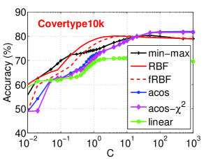
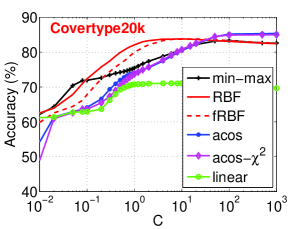
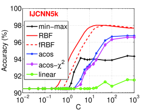
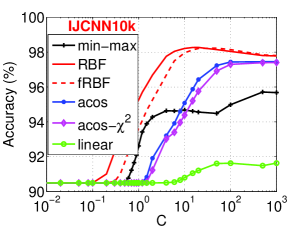
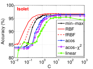
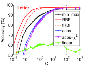
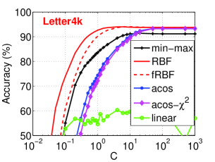
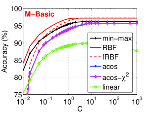
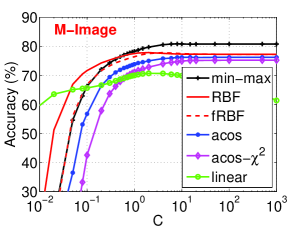
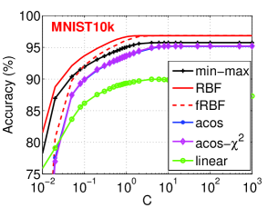
Figure 1: Test classification accuracies for 5 nonlinear kernels using $l_{2}$-regularized SVM (with a tuning parameter $C$, i.e., the x-axis). Each panel presents the results for one dataset (see data information in Table 1). For RBF/fRBF kernels (with a tuning parameter $\gamma$), at each $C$, we report the best accuracy from the results among all $\gamma$ values. See Figures 2 and 3 for results on more datasets. For comparison, we include the linear SVM results (green if color is available).

       

       

       

       

       

       

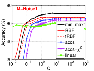
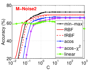
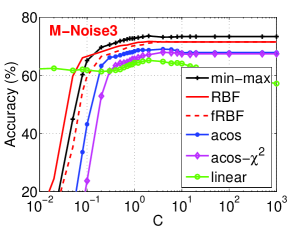
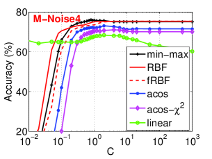
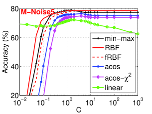
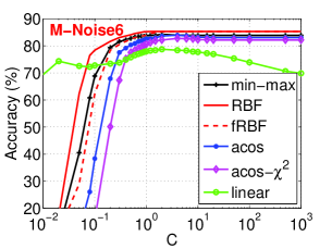
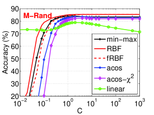
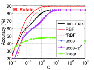
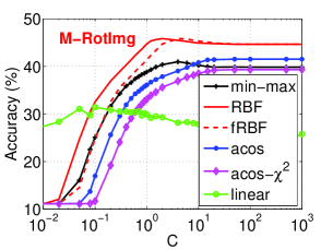
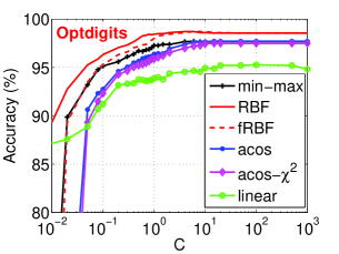
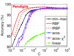
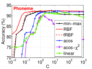
Figure 2: Test classification accuracies for 5 nonlinear kernels using $l_{2}$-regularized SVM.

       

       

       

       

       

       

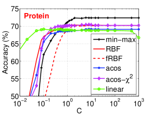
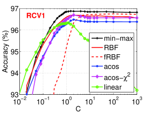
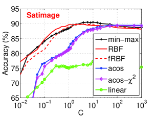
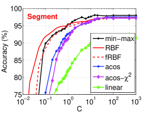
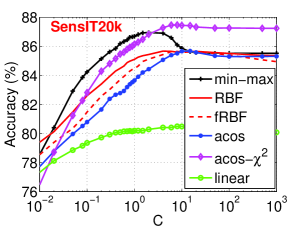
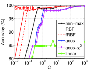
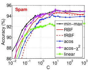
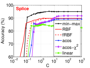
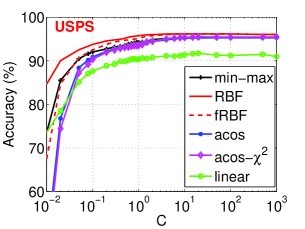
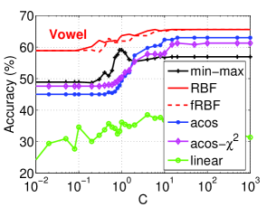
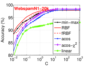
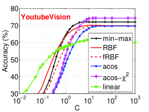
Figure 3: Test classification accuracies for 5 nonlinear kernels using $l_{2}$-regularized SVM.

3 Linearization of Nonlinear Kernels

It is known that a straightforward implementation of nonlinear kernels can be difficult for large datasets [2]. As mentioned earlier, for a small dataset with merely $60,000$ data points, the $60,000\times 60,000$ kernel matrix has $3.6\times 10^{9}$ entries. In practice, being able to linearize nonlinear kernels becomes very beneficial, as that would allow us to easily apply efficient linear algorithms in particular online learning [1]. Randomization is a popular tool for kernel linearization.

Since LIBSVM did not implement most of the nonlinear kernels in our study, we simply used the LIBSVM pre-computed kernel functionality in our experimental study as reported in Table 2. While this strategy ensures repeatability, it requires very large memory.

In the introduction, we have explained how to linearize these 5 types of nonlinear kernels. From practitioner’s perspective, while results in Table 2 are informative, they are not sufficient for guiding the choice of kernels. For example, as we will show, for some datasets, even though the RBF/fRBF kernels perform better than the min-max kernel in the kernel SVM experiments, their linearization algorithms require many more samples (i.e., large $k$) to reach the same accuracy as the linearization method (i.e., 0-bit CWS) for the min-max kernel.

3.1 RBF Kernel versus fRBF Kernel

We have explained how to linearize both the RBF kernel and the fRBF kernel in Introduction. For two normalized vectors $u,v\in\mathbb{R}^{D}$, we generate i.i.d. samples $r_{i}\sim N(0,1)$ and independent $w\sim uniform(0,2\pi)$. Let $x=\sum_{i=1}^{D}u_{i}r_{i}$ and $y=\sum_{i=1}^{D}vir_{i}$. Then we have

$$E\left(\cos(\sqrt{\gamma}x+w)\cos(\sqrt{\gamma}y+w)\right)=RBF(u,v;\gamma)$$

$$E\left(\cos(\sqrt{\gamma}x)\cos(\sqrt{\gamma}y)\right)=fRBF(u,v;\gamma)$$

In order to approximate the expectations with sufficient accuracies, we need to generate the samples $(x,y)$ many (say $k$) times. Typically $k$ has to be large. In our experiments, even though we use $k$ as large as 4096, it looks we will have to further increase $k$ in order to reach the accuracy of the original RBF/fRBF kernels (as in Table 2).

Figure 4 reports the linear SVM experiments on the linearized data for 10 datasets, for $k$ as large as 4096. We can see that, for most datasets, the linearized RBF and linearized fRBF kernels perform almost identically. For a few datasets, there are visible discrepancies but the differences are small. We repeat the experiments 10 times and the reported results are the averages. Note that we always use the best $\gamma$ values as provided in Table 2.

Together with the results on Table 2, the results as shown in Figure 4 allow us to conclude that the fRBF kernel can replace the RBF kernel and we can simplify the linearization algorithm by removing the additional random variable $w$.

       

       

       

       

       

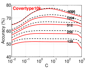
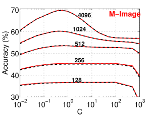
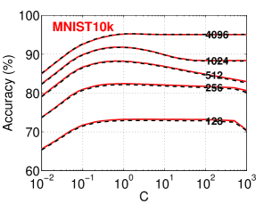
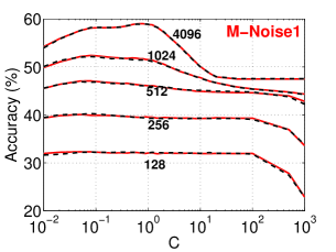
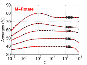
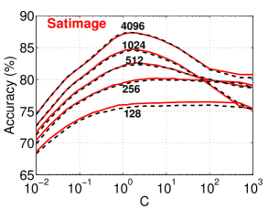
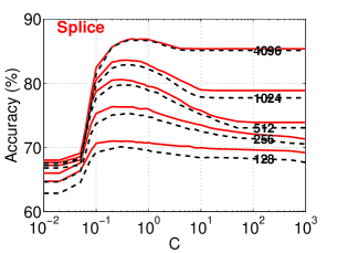
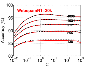
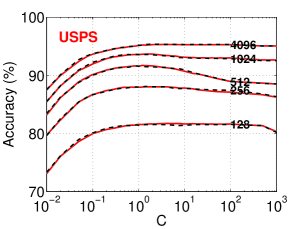
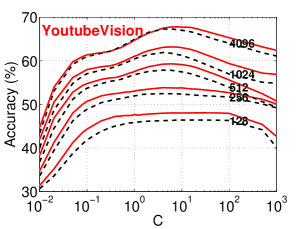
Figure 4: Classification accuracies of the linearized RBF (solid curves) and linearized fRBF (dashed curves) kernels, using LIBLINEAR. We report the results on 5 different $k$ (sample size) values: 128, 256, 512, 1024, 4096. For most datasets, both RBF and fRBF perform almost identically.

3.2 Min-max Kernel versus RBF/fRBF Kernels

Table 2 has shown that for quite a few datasets, the RBF/fRBF kernels outperform the min-max kernel. Now we compare their corresponding linearization algorithms. We adopt the 0-bit CWS [15] strategy and use at most 8 bits for storing each sample. See the Introduction and Appendix A for more details on consistent weighted sampling (CWS).

Figure 5 compares the linearization results of the min-max kernel with the results of the RBF kernel. We can see that the linearization algorithm for RBF performs very poorly when the sample size $k$ is small (e.g., $k<1024$). Even with $k=4096$, the accuracies still do not reach the accuracies using the original RBF kernel as reported in Table 2.

There is an interesting example. For the “M-Rotate” dataset, the original RBF kernel notably outperforms the original min-max kernel ($89.7\%$ versus $84.8\%$). However, as shown in Figure 5, even with 4096 samples, the accuracy of the linearized RBF kernel is still substantially lower than the accuracy of the linearized min-max kernel.

These observations motivate a useful future research: Can we develop an improved linearization algorithm for RBF/fRBF kernels which would require much fewer samples to reach good accuracies?

       

       

       

       

       

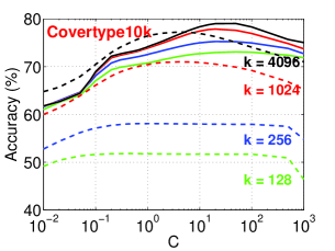
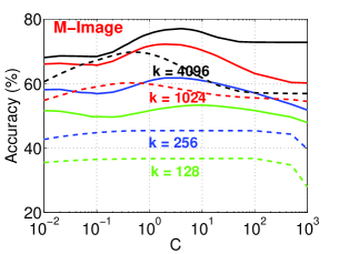
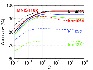
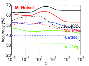
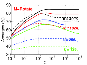
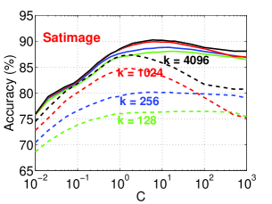
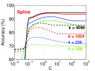
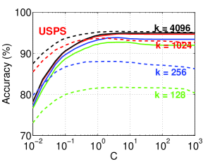
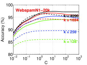
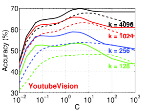
Figure 5: Classification accuracies of the linearized min-max kernel (solid curves) and linearized RBF (dashed curves) kernel, using LIBLINEAR. We report the results on 4 different $k$ (sample size) values: 128, 256, 1024, 4096. We only label the dashed curves. We can see that linearized RBF would require substantially more samples in order to reach the same accuracies as the linearized min-max method.

3.3 Min-max Kernel versus acos and acos-$\chi^{2}$ Kernels

As introduced at the beginning of the paper, sign Gaussian random projections and sign Cauchy random projections are the linearization methods for the acos kernel and the acos-$\chi^{2}$ kernel, respectively. Figures 6 and 7 compare them with 0-bit CWS, where we use “$\alpha=2$” for sign Gaussian projections and “$\alpha=1$” for sign Cauchy projections.

Again, like in Figure 5, we can see that the linearization method for the min-max kernel requires substantially few samples than the linearization methods for the acos and acos-$\chi^{2}$ kernels. Since both kernels show reasonably good performance (without linearization), This should also motivate us to pursue improved linearization algorithms for the acos and acos-$\chi^{2}$ kernels, as future research.

       

       

       

       

       

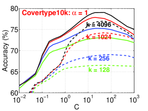
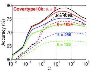
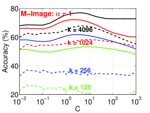
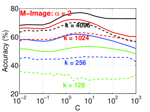
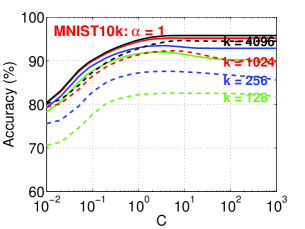
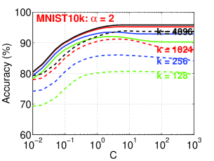
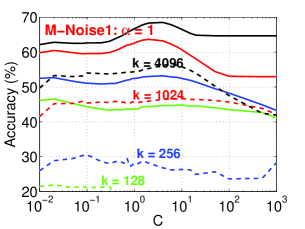
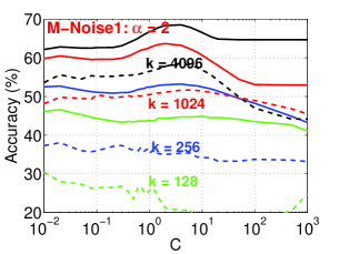
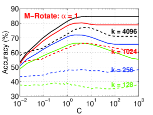
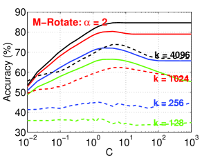
Figure 6: Classification accuracies of the linearized min-max kernel (solid curves) and acos (dashed curves) kernel (right panels, i.e., $\alpha=2$) and the acos-$\chi^{2}$ (dashed curves) kernel (left panels, i.e., $\alpha=1$), using LIBLINEAR. We report the results on 4 different $k$ (sample size) values: 128, 256, 1024, 4096. We only label the dashed curves. We can see that linearized acos and acos-$\chi^{2}$ kernels require substantially more samples in order to reach the same accuracies as the linearized min-max method.

       

       

       

       

       

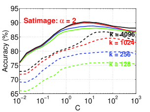
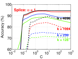
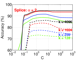
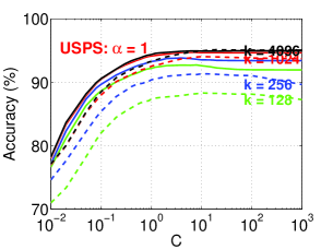
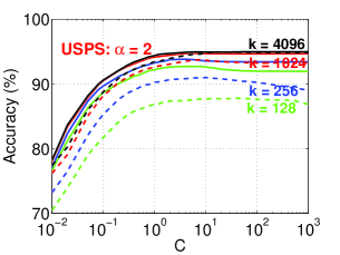
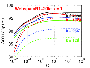
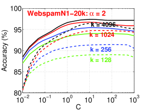
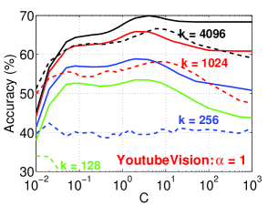
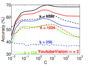
Figure 7: Classification accuracies of the linearized min-max kernel (solid curves) and acos (dashed curves) kernel (right panels, i.e., $\alpha=2$) and the acos-$\chi^{2}$ (dashed curves) kernel (left panels, i.e., $\alpha=1$), using LIBLINEAR. Again, we can see that linearized acos and acos-$\chi^{2}$ kernels require substantially more samples in order to reach the same accuracies as the linearized min-max method.

3.4 Comparisons on a Larger Dataset

Figure 8 provides the comparison study on the “WebspamN1” dataset, which has 175,000 examples for training and 175,000 examples for testing. It is too large for using the LIBSVM pre-computed kernel functionality in common workstations. On the other hand, we can easily linearize the nonlinear kernels and run LIBLINEAR on the transformed dataset.

The left panel of Figure 8 compares the results of linearization method (i.e., 0-bit CWS) for the min-max kernel with the results of the linearization method for the RBF kernel. The right panel compares 0-bit CWS with sign Gaussian random projections (i.e., $\alpha=2$). We do not present the results for $\alpha=1$ since they are quite similar. The plots again confirm that 0-bit CWS significantly outperforms the linearization methods for both the RBF kernel and the acos kernel.

       

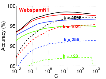
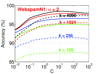
Figure 8: Experiments on a larger dataset. Left panel: Classification accuracies of the linearized min-max kernel (solid curves) and the linearized RBF (dashed curves) kernel. Right panel: Classification accuracies of the linearized min-max kernel (solid curves) and the linearized acos (dashed curves) kernel (i.e., $\alpha=2$). The linearization method for the min-max kernel (i.e., 0-bit CWS) substantially outperforms the linearization methods for the other two kernels.

4 Kernel Combinations

It is an interesting idea to combine kernels for better (or more robust) performance. One simple strategy is to use multiplication of kernels. For example, the following two new kernels

$$\text{MM-acos}(u,v)=\text{MM}(u,v)\times\text{acos}(u,v)$$ (14)

$$\text{MM-acos-}\chi^{2}(u,v)=\text{MM}(u,v)\times\text{acos-}\chi^{2}(u,v)$$ (15)

combine the min-max kernel with the acos kernel or the acos-$\chi^{2}$ kernel. They are still positive definite because they are the multiplications of positive definite kernels.

Table 3: Classification accuracies (in $\%$) of the two new kernels: MM-acos defined in (14) and MM-acos-$\chi^{2}$ defined in (15), as presented in the last two columns.

Dataset	min-max	acos	acos-$\chi^{2}$	MM-acos	MM-acos-$\chi^{2}$
Covertype10k	80.4	81.9	81.6	81.9	81.9
Covertype20k	83.3	85.3	85.0	85.3	85.3
IJCNN5k	94.4	96.9	96.6	95.6	95.4
IJCNN10k	95.7	97.5	97.4	96.2	96.1
Isolet	96.4	96.5	96.1	96.7	96.6
Letter	96.2	97.0	97.0	97.2	97.2
Letter4k	91.4	93.3	93.3	92.9	92.8
M-Basic	96.2	95.7	95.8	96.6	96.5
M-Image	80.8	76.2	75.2	81.0	80.8
MNIST10k	95.7	95.2	95.2	96.1	96.1
M-Noise1	71.4	65.0	64.0	71.0	70.8
M-Noise2	72.4	66.9	65.7	72.2	72.0
M-Noise3	73.6	69.0	68.0	73.9	73.5
M-Noise4	76.1	73.1	71.1	75.8	75.5
M-Noise5	79.0	76.6	74.9	78.7	78.5
M-Noise6	84.2	83.9	82.8	84.6	84.3
M-Rand	84.2	83.5	82.3	84.5	84.3
M-Rotate	84.8	84.5	84.6	86.5	86.4
M-RotImg	41.0	41.5	39.3	42.8	41.8
Optdigits	97.7	97.7	97.5	97.8	97.9
Pendigits	97.9	98.3	98.1	98.2	98.0
Phoneme	92.5	92.2	90.2	92.6	92.1
Protein	72.4	69.2	70.5	71.2	71.4
RCV1	96.9	96.5	96.7	96.8	96.8
Satimage	90.5	89.5	89.4	91.2	90.9
Segment	98.1	97.6	97.2	98.1	98.3
SensIT20k	86.9	85.7	87.5	87.1	87.3
Shuttle1k	99.7	99.7	99.7	99.7	99.7
Spam	95.0	94.2	95.2	94.9	95.0
Splice	95.2	89.2	91.7	95.9	95.7
USPS	95.3	95.3	95.5	95.5	95.5
Vowel	59.1	63.0	61.3	58.9	58.7
WebspamN1-20k	97.9	98.1	98.5	98.0	98.2
YoutubeVision	72.2	69.6	74.4	72.0	72.3

Table 3 presents the kernel SVM experiments for these two new kernels (i.e., the last two columns). We can see that for majority of the datasets, these two kernels outperform the min-max kernel. For a few datasets, the min-max kernel still performs the best (for example, “M-Noise1”); and on these datasets, the acos kernel and the acos-$\chi^{2}$ kernel usually do not perform as well. Overall, these two new kernels appear to be fairly robust combinations. Of course, the story will not be complete until we have also studied their corresponding linearization methods.

A recent study [14] explored the idea of combing the “resemblance” kernel with the linear kernel, designed only for sparse non-binary data. Since most of the datasets we experiment with are not sparse, we can not directly use the special kernel developed in [14].

Now we study the linearization methods for these two new kernels, which turn out to be easy. Take the MM-acos kernel as an example. We can separately and independently generate samples for the min-max kernel and the acos kernel. The sample for the min-max kernel can be viewed as a binary vector with one 1. For example, if the sample for the min-max kernel is $[0,\ 0,\ 1,\ 0]$ and the sample for the acos kernel is -1. Then we can encode the combined sample as $[0,\ 0,\ 0,\ 0,\ 1,\ 0,\ 0,\ 0]$. If the sample for the acos kernel is 1, then the combined vector becomes $[0,\ 0,\ 0,\ 0,\ 0,\ 1,\ 0,\ 0]$. Basically, if the $j$-th location in the vector corresponding to the original min-max sample is 1, then the combined vector will double the length and all the entries will be zero except the ($2j$-1)-th or ($2j$)-th location, depending on the sample value of acos kernel.

Clearly, the idea also applies for combining min-max kernel with RBF kernel. We just need to replace the “1” in the vector for the min-max kernel sample with the sample of the RBF kernel.

       

       

       

       

       

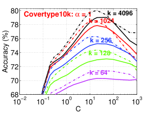
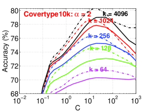
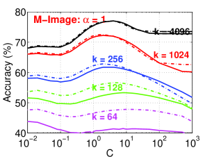
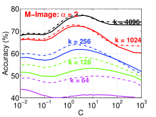
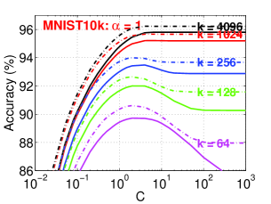
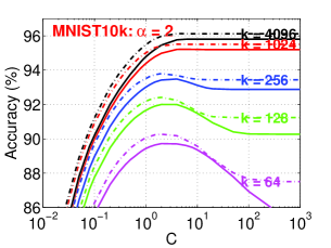
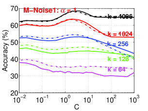
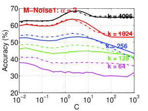
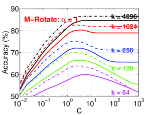
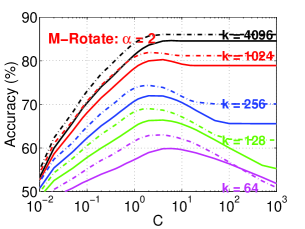
Figure 9: Classification accuracies of the linearized min-max kernel (solid curves), the MM-acos kernel (right panels ($\alpha=2$), dash-dotted curves), and the MM-acos-$\chi^{2}$ kernel (left panels ($\alpha=1$), dash-dotted curves), using LIBLINEAR. We report the results for $k\in\{64,128,256,1024,4096\}$. We can see that the linearized MM-acos kernel and the linearized MM-acos-$\chi^{2}$ kernel outperform the linearized min-max kernel when $k$ is not large.

       

       

       

       

       

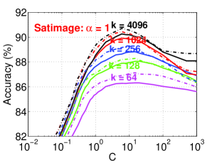
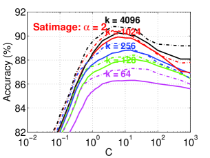
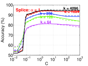
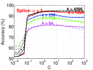
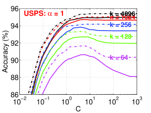
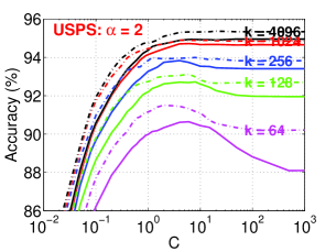
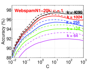
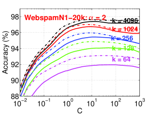
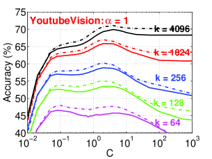
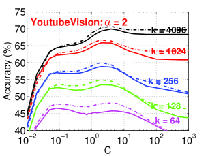
Figure 10: Classification accuracies of the linearized min-max kernel (solid curves), the MM-acos kernel (right panels ($\alpha=2$), dash-dotted curves), and the MM-acos-$\chi^{2}$ kernel (left panels ($\alpha=1$), dash-dotted curves), using LIBLINEAR. We report the results for $k\in\{64,128,256,1024,4096\}$.

Figure 9 and Figure 10 report the linear SVM results using linearized data for the MM-acos kernel (right panels) and the MM-acos-$\chi^{2}$ kernel (left panels), to compare with the results using linearized data for the min-max kernel (solid curves). We can see that the linearization methods for the MM-acos kernel and the MM-acos-$\chi^{2}$ kernel outperform the linearization method for the min-max kernel when $k$ is not large. These preliminary results are encouraging.

5 Conclusion

Nonlinear kernels can be potentially very useful if there are efficient (in both storage and memory) algorithms for computing them. It has been known that the RBF kernel, the acos kernel, and the acos-$\chi^{2}$ kernel can be linearized via randomization algorithms. There are two major aspects when we compare nonlinear kernels: (i) the accuracy of the original kernel; (ii) how many samples are needed in order to reach a good accuracy. In this paper, we try to address these two issues by providing an extensive empirical study on a wide variety of publicly available datasets.

To simplify the linearization procedure for the RBF kernel, we propose the folded RBF (fRBF) kernel and demonstrates that its performance (either with the original kernel or with linearization) is very similar to that of the RBF kernel. On the other hand, our extensive nonlinear kernel SVM experiments demonstrate that the RBF/fRBF kernels, even with the best-tuned parameters, do not always achieve the best accuracies. The min-max kernel (which is tuning-free) in general performs well (except for some very low dimensional datasets). The acos kernel and the acos-$\chi^{2}$ kernel also perform reasonably well.

Linearization is a crucial step in order to use nonlinear kernels for large-scale applications. Our experimental study illustrates that the linearization method for the min-max kernel, called “0-bit CWS”, performs well in that it does not require a large number of samples to reach a good accuracy. In comparison, the linearization methods for the RBF/fRBF kernels and the acos/acos-$\chi^{2}$ kernels typically require many more samples (e.g., $\geq 4096$).

Our study motivates two interesting research problems for future work: (i) how to design better (and still linearizable) kernels to improve the tuning-free kernels; (ii) how to improve the linearization algorithms for the RBF/fRBF kernels as well as the acos/acos-$\chi^{2}$ kernels, in order to reduce the required sample sizes. The interesting and simple idea of combing two nonlinear kernels by multiplication appears to be effective but we still hope to find an even better strategy in the future.

Another challenging task is to develop (linearizable) kernel algorithms to compete with (ensembles of) trees in terms of accuracy. It is known that tree algorithms are usually slow. Even though the parallelization of trees is easy, it will still consume excessive energy (e.g., electric power). One can see from [12, 13] that trees are in general perform really well in terms of accuracy and can be remarkably more accurate than other methods in some datasets (such as “M-Noise1” and “M-Image”). On top of the fundamental works [7, 6], the recent papers [12, 13] improved tree algorithms via two ideas: (i) an explicit tree-split formula using 2nd-order derivatives; (ii) a re-formulation of the classical logistic loss function which leads to a different set of first and second derivatives from textbooks. Ideally, it would be great to develop statistical machine learning algorithms which are as accurate as (ensembles of) trees and are as fast as linearizable kernels.

Appendix A Consistent Weighted Sampling

Input: Data vector $u$ = ($u_{i}\geq 0$, $i=1$ to $D$)

Output: Consistent uniform sample ($i^{*}$, $t^{*}$)

For $i$ from 1 to $D$

$r_{i}\sim Gamma(2,1)$,  $c_{i}\sim Gamma(2,1)$, $\beta_{i}\sim Uniform(0,1)$

$t_{i}\leftarrow\lfloor\frac{\log u_{i}}{r_{i}}+\beta_{i}\rfloor$,  $y_{i}\leftarrow\exp(r_{i}(t_{i}-\beta_{i}))$,  $a_{i}\leftarrow c_{i}/(y_{i}\exp(r_{i}))$

End For

$i^{*}\leftarrow arg\min_{i}\ a_{i}$,        $t^{*}\leftarrow t_{i^{*}}$

Algorithm 1 Consistent Weighted Sampling (CWS)

Given a data vector $u\in\mathbb{R}^{D}$, Alg. 1 (following [10]) provides the procedure for generating one CWS sample $(i^{*},t^{*}$). In order to generate $k$ such samples, we have to repeat the procedure $k$ times using independent random numbers $r_{i}$, $c_{i}$, $\beta_{i}$.

Appendix B Proof of Lemma 1

Let $t=\sqrt{\gamma}$. Using the bivariate normal density function, we obtain

$$E\left(\cos(tx)\cos(ty)\right)$$

$$= \int_{-\infty}^{\infty}\int_{-\infty}^{\infty}\cos(tx)\cos(ty)\frac{1}{2\pi}\frac{1}{\sqrt{1-\rho^{2}}}e^{-\frac{x^{2}+y^{2}-2\rho xy}{2(1-\rho^{2})}}dxdy$$

$$= \int_{-\infty}^{\infty}\int_{-\infty}^{\infty}\cos(tx)\cos(ty)\frac{1}{2\pi}\frac{1}{\sqrt{1-\rho^{2}}}e^{-\frac{x^{2}+y^{2}-2\rho xy+\rho^{2}x^{2}-\rho^{2}x^{2}}{2(1-\rho^{2})}}dxdy$$

$$= \int_{-\infty}^{\infty}\frac{1}{2\pi}\frac{1}{\sqrt{1-\rho^{2}}}e^{-\frac{x^{2}}{2}}\cos(tx)dx\int_{-\infty}^{\infty}\cos(ty)e^{-\frac{(y-\rho x)^{2}}{2(1-\rho^{2})}}dy$$

$$= \int_{-\infty}^{\infty}\frac{1}{2\pi}e^{-\frac{x^{2}}{2}}\cos(tx)dx\int_{-\infty}^{\infty}\cos(ty\sqrt{1-\rho^{2}}+t\rho x)e^{-y^{2}/2}dy$$

$$= \int_{-\infty}^{\infty}\frac{1}{2\pi}e^{-\frac{x^{2}}{2}}\cos(tx)\cos(t\rho x)dx\int_{-\infty}^{\infty}\cos(ty\sqrt{1-\rho^{2}})e^{-y^{2}/2}dy$$

$$= \int_{-\infty}^{\infty}\frac{1}{2\pi}e^{-\frac{x^{2}}{2}}\cos(tx)\cos(t\rho x)\sqrt{2\pi}e^{-t^{2}\frac{1-\rho^{2}}{2}}dx$$

$$= \frac{1}{\sqrt{2\pi}}e^{-t^{2}\frac{1-\rho^{2}}{2}}\int_{-\infty}^{\infty}e^{-\frac{x^{2}}{2}}\cos(tx)\cos(t\rho x)dx$$

$$= \frac{1}{\sqrt{2\pi}}e^{-t^{2}\frac{1-\rho^{2}}{2}}\frac{\sqrt{2\pi}}{2}\left[e^{-t^{2}\frac{(1-\rho)^{2}}{2}}+e^{-t^{2}\frac{(1+\rho)^{2}}{2}}\right]$$

$$= \frac{1}{2}e^{-t^{2}(1-\rho)}+\frac{1}{2}e^{-t^{2}(1+\rho)}$$

References

- [1] L. Bottou. http://leon.bottou.org/projects/sgd.
- [2] L. Bottou, O. Chapelle, D. DeCoste, and J. Weston, editors. Large-Scale Kernel Machines. The MIT Press, Cambridge, MA, 2007.
- [3] O. Chapelle, P. Haffner, and V. N. Vapnik. Support vector machines for histogram-based image classification. IEEE Transactions on Neural Networks, 10(5):1055–1064, 1999.
- [4] M. S. Charikar. Similarity estimation techniques from rounding algorithms. In STOC, pages 380–388, Montreal, Quebec, Canada, 2002.
- [5] R.-E. Fan, K.-W. Chang, C.-J. Hsieh, X.-R. Wang, and C.-J. Lin. Liblinear: A library for large linear classification. Journal of Machine Learning Research, 9:1871–1874, 2008.
- [6] J. H. Friedman. Greedy function approximation: A gradient boosting machine. The Annals of Statistics, 29(5):1189–1232, 2001.
- [7] J. H. Friedman, T. J. Hastie, and R. Tibshirani. Additive logistic regression: a statistical view of boosting. The Annals of Statistics, 28(2):337–407, 2000.
- [8] M. X. Goemans and D. P. Williamson. Improved approximation algorithms for maximum cut and satisfiability problems using semidefinite programming. Journal of ACM, 42(6):1115–1145, 1995.
- [9] T. J. Hastie, R. Tibshirani, and J. H. Friedman. The Elements of Statistical Learning:Data Mining, Inference, and Prediction. Springer, New York, NY, 2001.
- [10] S. Ioffe. Improved consistent sampling, weighted minhash and L1 sketching. In ICDM, pages 246–255, Sydney, AU, 2010.
- [11] H. Larochelle, D. Erhan, A. C. Courville, J. Bergstra, and Y. Bengio. An empirical evaluation of deep architectures on problems with many factors of variation. In ICML, pages 473–480, Corvalis, Oregon, 2007.
- [12] P. Li. Abc-boost: Adaptive base class boost for multi-class classification. In ICML, pages 625–632, Montreal, Canada, 2009.
- [13] P. Li. Robust logitboost and adaptive base class (abc) logitboost. In UAI, 2010.
- [14] P. Li. CoRE kernels. In UAI, Quebec City, CA, 2014.
- [15] P. Li. 0-bit consistent weighted sampling. In KDD, Sydney, Australia, 2015.
- [16] P. Li, G. Samorodnitsky, and J. Hopcroft. Sign cauchy projections and chi-square kernel. In NIPS, Lake Tahoe, NV, 2013.
- [17] M. Manasse, F. McSherry, and K. Talwar. Consistent weighted sampling. Technical Report MSR-TR-2010-73, Microsoft Research, 2010.
- [18] A. Rahimi and B. Recht. andom features for large-scale kernel machines. In NIPS, 2007.
- [19] W. Rudin. Fourier Analysis on Groups. John Wiley & Sons, New York, NY, 1990.
- [20] B. Schiele and J. L. Crowley. Object recognition using multidimensional receptive field histograms. In ECCV, pages 610–619, Helsinki, Finland, 1996.