Finding Planet Nine: a Monte Carlo approach

Abstract

Planet Nine is a hypothetical planet located well beyond Pluto that has been proposed in an attempt to explain the observed clustering in physical space of the perihelia of six extreme trans-Neptunian objects or ETNOs. The predicted approximate values of its orbital elements include a semimajor axis of 700 au, an eccentricity of 0.6, an inclination of 30°, and an argument of perihelion of 150°. Searching for this putative planet is already under way. Here, we use a Monte Carlo approach to create a synthetic population of Planet Nine orbits and study its visibility statistically in terms of various parameters and focusing on the aphelion configuration. Our analysis shows that, if Planet Nine exists and is at aphelion, it might be found projected against one out of four specific areas in the sky. Each area is linked to a particular value of the longitude of the ascending node and two of them are compatible with an apsidal anti-alignment scenario. In addition and after studying the current statistics of ETNOs, a cautionary note on the robustness of the perihelia clustering is presented.

1 Introduction

Batygin & Brown (2016) have predicted the existence of a massive planet well beyond Pluto in order to explain the observed clustering in physical space of the perihelia of the extreme trans-Neptunian objects or ETNOs (90377) Sedna, 2004 VN₁₁₂, 2007 TG₄₂₂, 2010 GB₁₇₄, 2012 VP₁₁₃, and 2013 RF₉₈. Such clustering is fairly obvious in terms of the values of their arguments of perihelion in Table 1 and, even more clear, positionally in Table 2 and Fig. 1 at about 3^h in right ascension, $\alpha$, and 0°in declination, $\delta$. The putative object responsible for inducing this clustering has been provisionally denominated Planet Nine. Batygin & Brown (2016) have provided tentative values for the orbital parameters of the proposed 10 Earth masses planet (semimajor axis, $a=700$ au, eccentricity, $e=0.6$, inclination, $i=30$°, and argument of perihelion, $\omega=150$°) and discussed its possible location in the sky. Planet Nine as characterized by Batygin & Brown (2016) is expected to exhibit a magnitude $V$ in the range 16–21 at perihelion and 20–25 at aphelion. Detailed modelling by Linder & Mordasini (2016) gives a magnitude $V$ from the reflected light of 23.7 at aphelion.

In principle, searching for this putative planet is feasible for currently active moving object surveys and it is already under way. For slow-moving objects, most active surveys can record candidates brighter than $V=22$ mag (see e.g. Harris & D’Abramo 2015). The faintest natural moving object observation performed so far corresponds to $V=26.7$ mag for asteroid 2008 LG₂ (Micheli et al. 2015) and the faintest objects observable with 8-m class telescopes have about 27. V774104 was discovered with magnitude 24 at 103 au (Sheppard, Trujillo & Tholen 2015). Detection of moving objects not only depends on their apparent magnitude but on their rate of motion as well (see e.g. Harris & D’Abramo 2015). However, with an average daily motion of nearly 1 arcsec d^-1 at perihelion and almost 0.06 arcsec d^-1 at aphelion, this should be a non-issue for Planet Nine; the object’s sky motion is far too slow. Fortunately, its shifting with respect to background stars due to parallax as the Earth moves around the Sun could be as high as 3 arcsec d^-1 at aphelion (V774104 was identified via parallax, not daily motion). In any case, if Planet Nine currently moves projected against a rich stellar background (a bright section of the Milky Way galaxy for instance) and/or its apparent magnitude is $>22$ in $V$, its eventual identification could be particularly challenging.

The Planet Nine hypothesis presents a suitable and robust scenario to explain the orbital properties of six ETNOs, but it may not be adequate to account for the apparent clustering of arguments of perihelion around 0°(Trujillo & Sheppard 2014) and inclination around 20°(de la Fuente Marcos & de la Fuente Marcos 2014) observed for ETNOs with values of the semimajor axis in the range 150–250 au. A number of scenarios aimed at explaining the available observational evidence have been proposed since the discovery of 2012 VP₁₁₃ (Trujillo & Sheppard 2014). They include the possible existence of one (Trujillo & Sheppard 2014; Gomes, Soares & Brasser 2015; Malhotra, Volk & Wang 2016) or more trans-Plutonian planets (de la Fuente Marcos & de la Fuente Marcos 2014; de la Fuente Marcos, de la Fuente Marcos & Aarseth 2015), capture of ETNOs within the Sun’s natal open star cluster (Jílková et al. 2015), stellar encounters (Brasser & Schwamb 2015; Feng & Bailer-Jones 2015), being a by-product of Neptune’s migration (Brown & Firth 2016) or the inclination instability (Madigan & McCourt 2016), and being the result of Milgromian dynamics (Paučo & Klačka 2016). In any case, trans-Plutonian planets —if they do exist— cannot be too massive or bright (Iorio 2014; Luhman 2014; Cowan, Holder & Kaib 2016; Fienga et al. 2016; Ginzburg, Sari & Loeb 2016; Linder & Mordasini 2016) to have escaped detection during the last two decades of surveys and astrometric studies; masses close to or below those of Uranus or Neptune are most likely. Trans-Plutonian planets may have been scattered out of the region of the giant planets early in the history of the Solar system (see e.g. Bromley & Kenyon 2014) or even captured from another planetary system (Li & Adams 2016), but planets similar to Uranus or Neptune (super-Earths) may also form at 125–250 au from the Sun (Kenyon & Bromley 2015). The putative existence of trans-Plutonian planets may have a role on models aimed at explaining periodic mass extinctions (Whitmire 2016).

The study of the visibility of the ETNOs carried out in de la Fuente Marcos & de la Fuente Marcos (2014) revealed an intrinsic bias in declination induced by our observing point on Earth: the vast majority must reach perihelion (i.e. perigee) at declinations in the range $-$24°to 24°. Here, we study the visibility of a synthetic population of Planet Nine virtual orbits from the Earth to uncover possible biases that may affect the detectability of such object if it exists. This Letter is organized as follows. Section 2 is a review of ETNOs statistics that includes a cautionary note regarding the perihelia clustering identified in Batygin & Brown (2016). Our Monte Carlo methodology is briefly reviewed in Section 3. The distribution in equatorial coordinates of Planet Nine virtual orbits at aphelion is studied in Section 4. Section 5 repeats the analysis for the location of Planet Nine in Fienga et al. (2016). Results are discussed in Section 6 and conclusions are summarized in Section 7.

Table 1: Various orbital parameters —$q=a(1-e)$, $Q=a(1+e)$, $\varpi=\Omega+\omega$, $P$ is the orbital period, $\Omega^{*}$ and $\omega^{*}$ are $\Omega$ and $\omega$ in the interval ($-\pi$, $\pi$) instead of the regular (0, 2$\pi$)— for the 16 objects discussed in this Letter. The statistical parameters are Q₁, first quartile, Q₃, third quartile, IQR, interquartile range, OL, lower outlier limit (Q${}_{1}-1.5$IQR), and OU, upper outlier limit (Q${}_{3}+1.5$IQR); see the text for additional details. (Epoch: 2457400.5, 2016-January-13.0 00:00:00.0 UT. J2000.0 ecliptic and equinox. Source: Jet Propulsion Laboratory Small-Body Database. Data retrieved on 27 February 2016.)

Object	$a$ (au)	$e$	$i$ (°)	$\Omega$ (°)	$\omega$ (°)	$\varpi$ (°)	$q$ (au)	$Q$ (au)	$P$ (yr)	$\Omega^{*}$ (°)	$\omega^{*}$ (°)
(82158) 2001 FP185	226.3448	0.8486685	30.75720	179.3004	6.9787	186.2791	34.2531	418.4364	3405.367	179.3004	6.9787
(90377) Sedna	507.5603	0.8501824	11.92872	144.5463	311.4614	96.0077	76.0415	939.0792	11435.094	144.5463	$-$48.5386
(148209) 2000 CR105	227.9513	0.8057223	22.71773	128.2463	317.2193	85.4656	44.2859	411.6168	3441.687	128.2463	$-$42.7807
(445473) 2010 VZ98	152.7794	0.7753635	4.50950	117.4524	313.8953	71.3477	34.3198	271.2389	1888.449	117.4524	$-$46.1047
2002 GB32	215.7621	0.8362043	14.17368	176.9791	36.9855	213.9646	35.3409	396.1834	3169.356	176.9791	36.9855
2003 HB57	164.6181	0.7685925	15.47644	197.8293	10.7805	208.6098	38.0939	291.1424	2112.149	-162.1707	10.7805
2003 SS422	193.8328	0.7966122	16.80783	151.1119	209.8843	0.9962	39.4232	348.2424	2698.666	151.1119	$-$150.1157
2004 VN112	321.0199	0.8525664	25.56295	66.0107	327.1707	33.1814	47.3291	594.7106	5751.830	66.0107	$-$32.8293
2005 RH52	151.1376	0.7420410	20.46234	306.1711	32.3890	338.5601	38.9873	263.2879	1858.091	-53.8289	32.3890
2007 TG422	492.7277	0.9277916	18.58697	112.9515	285.7968	38.7483	35.5791	949.8764	10937.517	112.9515	$-$74.2032
2007 VJ305	188.3373	0.8131705	12.00306	24.3834	338.3611	2.7445	35.1870	341.4876	2584.715	24.3834	$-$21.6389
2010 GB174	371.1183	0.8687090	21.53812	130.6119	347.8124	118.4243	48.7245	693.5121	7149.518	130.6119	$-$12.1876
2012 VP113	259.3002	0.6896024	24.04680	90.8179	293.7168	24.5346	80.4862	438.1142	4175.538	90.8179	$-$66.2832
2013 GP136	152.4968	0.7303547	33.48578	210.7142	42.1284	252.8426	41.1201	263.8736	1883.213	-149.2858	42.1284
2013 RF98	309.0738	0.8826022	29.61402	67.5205	316.4991	24.0196	36.2846	581.8631	5433.774	67.5205	$-$43.5009
2015 SO20	162.7035	0.7961710	23.44153	33.6221	354.9699	28.5920	33.1637	292.2434	2075.409	33.6221	$-$5.0301
Mean	256.0478	0.8115221	20.31954	133.6418	221.6281	107.7699	43.6637	468.4318	4375.023	66.1418	$-$25.8719
Standard deviation	115.6941	0.0616087	7.71647	71.9552	140.3086	102.2955	14.3016	225.1645	3077.676	105.7150	48.9934
Median	221.0535	0.8094464	21.00023	129.4291	302.5891	78.4066	38.5406	403.9001	3287.362	101.8847	$-$27.2341
Q1	164.1395	0.7736707	15.15075	84.9935	40.8427	27.5777	35.3024	291.9681	2102.964	31.3124	$-$46.7132
Q3	312.0603	0.8507784	24.42584	177.5594	319.7071	191.8618	45.0467	585.0750	5513.288	134.0955	7.9291
IQR	147.9209	0.0771077	9.27509	92.5659	278.8645	164.2841	9.7443	293.1068	3410.324	102.7831	54.6423
OL	$-$57.7418	0.6580092	1.23812	$-$53.8553	$-$377.4541	$-$218.8485	20.6860	$-$147.6921	$-$3012.521	$-$122.8622	$-$128.6766
OU	533.9416	0.9664399	38.33846	316.4082	738.0039	438.2880	59.6631	1024.7352	10628.773	288.2701	89.8926

Table 2: Equatorial coordinates, apparent magnitudes (with filter if known) at discovery time, absolute magnitude, and $\omega$ for the 16 objects discussed in this Letter. (J2000.0 ecliptic and equinox. Source: Minor Planet Center —MPC— Database.)

Object	$\alpha$ (h:m:s)	$\delta$ (°:′:″)	$m$ (mag)	$H$ (mag)	$\omega$ (°)
82158	11:57:50.69	+00:21:42.7	22.2 (R)	6.0	6.77
Sedna	03:15:10.09	+05:38:16.5	20.8 (R)	1.5	311.19
148209	09:14:02.39	+19:05:58.7	22.5 (R)	6.3	317.09
445473	02:08:43.575	+08:06:50.90	20.3 (R)	5.0	313.80
2002 GB32	12:28:25.94	$-$00:17:28.4	21.9 (R)	7.7	36.89
2003 HB57	13:00:30.58	$-$06:43:05.4	23.1 (R)	7.4	10.64
2003 SS422	23:27:48.15	$-$09:28:43.4	22.9 (R)	7.1	209.98
2004 VN112	02:08:41.12	$-$04:33:02.1	22.7 (R)	6.4	327.23
2005 RH52	22:31:51.90	+04:08:06.1	23.8 (g)	7.8	32.59
2007 TG422	03:11:29.90	$-$00:40:26.9	22.2	6.2	285.84
2007 VJ305	00:29:31.74	$-$00:45:45.0	22.4	6.6	338.53
2010 GB174	12:38:29.365	+15:02:45.54	25.09 (g)	6.5	347.53
2012 VP113	03:23:47.159	+01:12:01.65	23.1 (r)	4.1	293.97
2013 GP136	14:09:40.000	$-$11:30:08.47	23.5 (r)	6.6	42.16
2013 RF98	02:29:07.61	$-$04:56:34.6	23.5 (z)	8.6	316.55
2015 SO20	01:01:17.301	$-$03:11:00.81	21.4 (R)	6.4	354.97

2 ETNOs: current statistics

In Trujillo & Sheppard (2014) the ETNOs are defined as asteroids with semimajor axis greater than 150 au and perihelion greater than 30 au. At present, there are 16 known ETNOs (see Tables 1 and 2 for relevant data). The descriptive statistics of this sample are included in Table 1; in this table, unphysical values are displayed for completeness. From these results it is obvious that the strongest clustering is observed in $e$ and $i$. As pointed out in de la Fuente Marcos & de la Fuente Marcos (2014), the clustering in $e$ can be the result of observational bias but the one in $i$ cannot be explained as resulting from selection effects, it must have a dynamical origin. As the one in $e$, the clustering in the values of the perihelion distance may be explained as a selection effect. It is also clear that the new additions to the ETNO group since the discovery of 2012 VP₁₁₃ follow the trends already identified in 2014; in particular, the orbits of 2004 VN₁₁₂ and 2013 RF₉₈ are alike. However, we would like to point out a potentially important issue even if the ETNO sample is still small. In statistics, outliers are often defined as observations that fall below Q${}_{1}-1.5$ IQR or above Q${}_{3}+1.5$ IQR, where Q₁ is the first or lower quartile, Q₃ is the third or upper quartile, and IQR is the interquartile range or difference between the upper and lower quartiles. In general, there are no outliers among the ETNOs (e.g. 2003 SS₄₂₂ is an outlier in terms of $\omega^{*}$, see Table 1), but both (90377) Sedna and 2012 VP₁₁₃ are statistical outliers in terms of perihelion distance, $q$. The upper boundary for outliers in $q$ is 59.7 au; the values of the perihelion distance of both Sedna and 2012 VP₁₁₃ are well above this upper limit. Sedna is also an outlier in terms of orbital period. The sample is small but this fact may be signalling a different dynamical context for these two objects. It is statistically possible that Sedna and 2012 VP₁₁₃ are members of a separate dynamical class within the ETNOs and therefore be subjected to a different set of perturbations.

The scenario in which trans-Plutonian planets keep the values of the orbital parameters of the ETNOs in check thanks to a particular case of the Kozai mechanism (Kozai 1962) discussed in Trujillo & Sheppard (2014), de la Fuente Marcos & de la Fuente Marcos (2014) or de la Fuente Marcos et al. (2015) and the resonant coupling mechanism described in Batygin & Brown (2016) create dynamical pathways that in some cases may deliver objects to high inclination or even retrograde orbits. In principle, the mechanism detailed in de la Fuente Marcos et al. (2015) can also produce objects with orbits at steeply inclined angles, it already does it for Jupiter. On the other hand, the scenarios described in de la Fuente Marcos et al. (2015) and Batygin & Brown (2016) are not incompatible, and the Kozai mechanism can operate at high eccentricities (see e.g. Naoz 2016) when the value of the relative longitude of perihelion, $\Delta\varpi$, librates about 180°(apsidal anti-alignment). A hypothetical Planet Nine may induce Kozai-like behaviour, i.e. libration of the value of the argument of perihelion of the ETNOs that reproduces the observed clustering. The currently known ETNOs probably represent evolutionary steps within dynamical tracks and some of them are more dynamically evolved than others. The presence of statistical outliers could be a sign of this.

3 A Monte Carlo approach

The study of the visibility of a set of orbits with parameters defined within some boundary values is a statistical problem well suited to apply Monte Carlo techniques (Metropolis & Ulam 1949; Press et al. 2007). A representative sample of the set of orbits under study is systematically explored so the regions in the sky with optimal visibility (highest probability) can be determined; in our case, the equations of the orbits of both the Earth and Planet Nine under the two-body approximation (e.g. Murray & Dermott 1999) are sampled to find the minimum and maximum distance between the Earth and Planet Nine. This technique was used in de la Fuente Marcos & de la Fuente Marcos (2014) to analyse the visibility of the ETNOs, and the details and further references are given there. Using a Monte Carlo approach, we generate a synthetic population of Planet Nines with semimajor axis, $a\in$ (650, 750) au, eccentricity, $e\in$ (0.55, 0.65), inclination, $i\in$ (25, 35)°, longitude of the ascending node, $\Omega\in$ (0, 360)°, and argument of perihelion, $\omega\in$ (140, 160)°as no explicit value of $\Omega$ is given in Batygin & Brown (2016). We assume that the orbits of the multiple instances of Planet Nine are uniformly distributed in orbital parameter space. Ten million test orbits have been studied focusing on the visibility at aphelion. The analyses in Fienga et al. (2016) and Linder & Mordasini (2016) strongly disfavour a present-day Planet Nine located at perihelion.

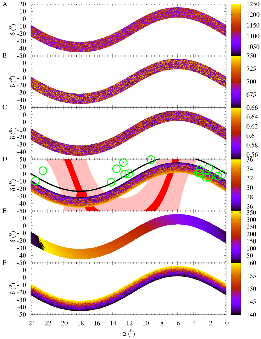
Figure 1: Distribution in equatorial coordinates of the studied orbits at aphelion as a function of various orbital elements and parameters. As a function of the value of the aphelion distance (panel A), of $a$ (panel B), of $e$ (panel C), of $i$ (panel D), of $\Omega$ (panel E), and of $\omega$ (panel F). The green circles in panel D give the location at discovery of all the known ETNOs. Also in panel D, the Galactic disc is arbitrarily defined as the region confined between galactic latitude $-5$°and 5°(in red), the position of the Galactic Centre is represented by a filled red circle, the region enclosed between galactic latitude $-30$°and 30°appears in pink, and the ecliptic appears in black.

The distribution in equatorial coordinates of the set of studied orbits is presented in Fig. 1. In this figure, the value of the parameter in the appropriate units is colour coded following the scale printed on the associated colour box. In panel D (inclination), the locations of the Galactic disc and centre are indicated. The background stellar density is the highest towards these regions in the sky. The distribution of aphelion distances, semimajor axes and eccentricities is rather uniform. The distribution in inclination and argument of perihelion depends on the declination; those orbits with higher values of the inclination reach aphelion at lower declinations, the same behaviour is observed for the ones with lower values of the argument of perihelion. The distribution in longitude of the ascending node depends on the right ascension; orbits with $\Omega\sim$0°reach aphelion at $\alpha\sim$23^h, the ones with $\Omega\sim$ 90°at $\alpha\sim$5^h, and those with $\Omega\sim$270°reach aphelion at $\alpha\sim$17^h. In any case, orbits reach perihelion at declination in the range $-$20°to 50°(not shown) and aphelion in the range $-$50°to 20°. This is markedly different from the bias found for the ETNOs in de la Fuente Marcos & de la Fuente Marcos (2014); i.e. searching for Planet Nine is not expected to increase the discovery rate of ETNOs and searching for ETNOs is not going to make a direct detection of Planet Nine more likely (indirectly yes, by improving the values of its putative orbital elements).

4 Planet Nine at aphelion

Detection of Planet Nine would be much easier if it is close to perihelion at present, but the analysis of Cassini radio ranging data carried out in Fienga et al. (2016) strongly suggests that Planet Nine as characterized by Batygin & Brown (2016) cannot be at perihelion. This conclusion is consistent with the analysis of its expected photometric properties in e.g. Linder & Mordasini (2016). A location in or near aphelion is however compatible with both the analysis of planetary ephemerides and the outcome of the many surveys completed in recent years. If Planet Nine is currently near aphelion, its declination will be in the range $-$50°to 20°(see Fig. 1), but not all the values of $\delta$ are equally probable. Figure 2 shows that the distribution is somewhat uniform in right ascension, but the probability of finding an orbit reaching aphelion at declinations in the ranges ($-$40, $-$30)°and (0, 10)°is nearly 1.7 times higher than that of doing it in the range ($-$30, 0)°. The effect of the bias in declination is analysed in more detail in Fig. 3. Locations near the Galactic Centre are possible if $\Omega\sim 300\degr$; the Galactic Centre is approximately at $\alpha\sim 17\aas@@fstack{h}7$ and $\delta\sim-29\degr$. A more exhaustive analysis shows that if $\delta\in(5,7)\degr$ then $\Omega\in(145,155)\degr$ and $\alpha\in(8,9)^{\rm h}$, which is located in Hydra and away from the main bulk of the Milky Way. Unfortunately, another optimal solution is possible —albeit slightly less probable— if $\delta\in(-35,-33)\degr$ then $\Omega\in(265,275)\degr$ and $\alpha\in(15.5,16.5)^{\rm h}$, which is located towards the Galactic bulge between the constellations of Scorpius and Lupus, but relatively far from the Galactic Centre. These two areas are associated with values of $\Omega$ that give $\Delta\varpi$ equal to 180°($\Omega=150$°) and 60°($\Omega=270$°), respectively. This second value is inconsistent with the pseudo resonant scenario described in Batygin & Brown (2016). Figures 2 and 3 show that two other solutions are possible but less probable. One with $\delta\in(5,7)\degr$, $\Omega\sim 100$°and $\alpha\in(3.5,4.5)^{\rm h}$ —in Taurus— and the second one with $\delta\in($-$35,$-$33)\degr$, $\Omega\sim 310$°and $\alpha\in(20,21)^{\rm h}$ —between Microscopium and Sagittarius. The solution with $\Omega\sim 100$°is favoured by Batygin and Brown (2016; see footnote 1) and subsequently by Fienga et al. (2016). Such solution gives a value of $\Delta\varpi\sim 200$°which is also consistent with apsidal anti-alignment.

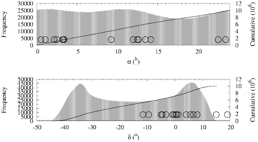
Figure 2: Frequency distribution in equatorial coordinates (right ascension, top panel, and declination, bottom panel) of the studied virtual orbits at aphelion. The distribution is somewhat uniform in right ascension and shows two maxima for declinations in the ranges ($-$40, $-$30)°and (0, 10)°. In this and subsequent figures, the number of bins is 2 $n^{1/3}$, where $n$ is the number of virtual orbits plotted, error bars are too small to be seen. The black circles correspond to objects in Table 2.

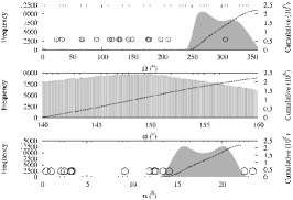
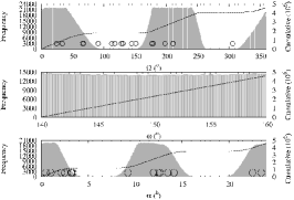
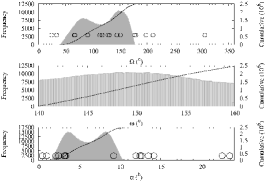
Figure 3: Frequency distribution in $\Omega$ (top panels), $\omega$ (middle panels), and right ascension (bottom panels) of virtual orbits with $\delta$ in the ranges ($-$40, $-$30)°(left-hand panels), ($-$30, 0)°(central panels), and (0, 10)°(right-hand panels). The black circles correspond to objects in Tables 1 and 2.

5 Cassini hints: Fienga et al. (2016)

Fienga et al. (2016) have carried out an analysis of Cassini radio ranging data. Their extrapolation of the Cassini data indicates that Planet Nine as characterised by Batygin & Brown (2016) cannot exist in the interval of true anomaly ($-$132, 106.5)°. This automatically excludes the perihelion (see their fig. 6). The aphelion is included in the uncertainty zone where the Cassini data do not provide any constraints, i.e. the residuals are compatible with zero. Fienga et al. (2016) indicate that from the point of view of the Cassini residuals, the most probable position of Planet Nine —assuming a value of $\Omega=113$°— is at true anomaly equal to 117.8°${}^{+11\degr}_{-10\degr}$. An analysis similar to that in Section 3 gives Fig. 4; this prediction places Planet Nine at $\alpha\sim 2^{\rm h}$ and $\delta\sim-20\degr$, in Cetus.

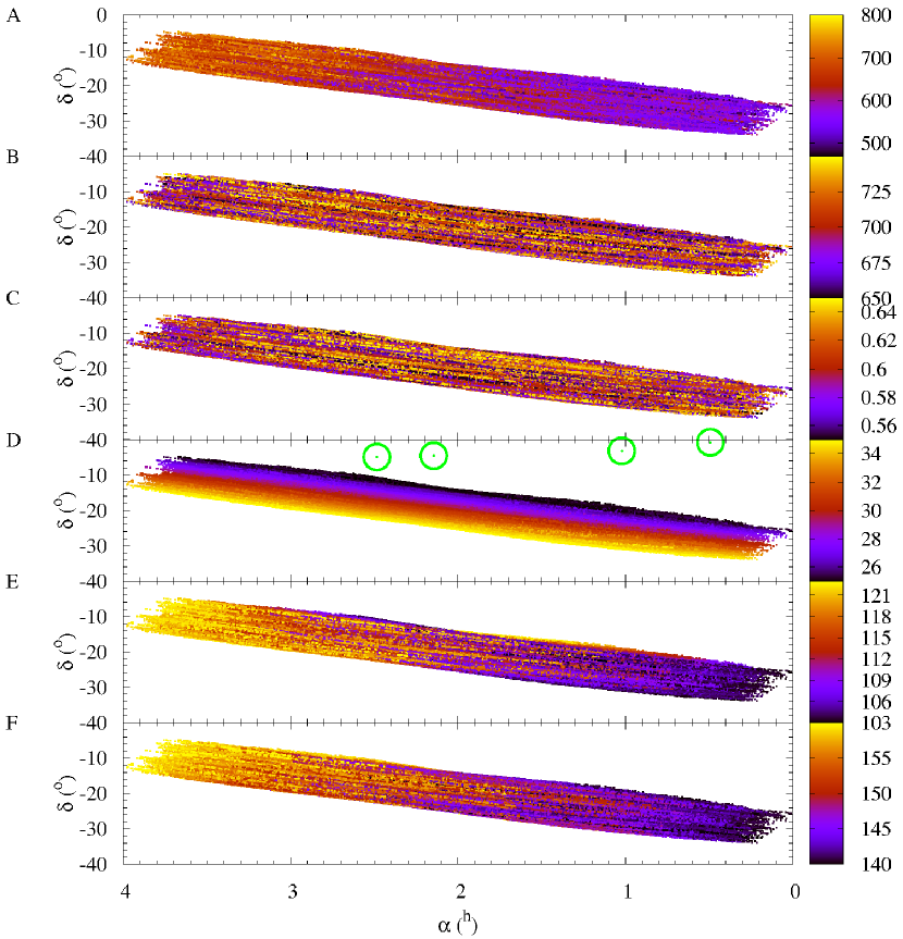
Figure 4: As Fig. 1 but for the orbital solution in Fienga et al. (2016). Here, panel A shows the value of the geocentric distance.

6 Discussion

The Planet Nine hypothesis represents an exciting opportunity to survey the outskirts of the Solar system with a purpose and improve our current knowledge of that distant region as well as of testing the correctness of models and long-standing assumptions. Our visibility analyses provide clues on the most probable location of the putative planet given a set of assumed orbital parameters based on the published data. The aphelion configuration gives two preferred present locations with nearly the same degree of probability and two others with lower probability. If any of the assumed parameters is grossly in error, the preferred locations computed via Monte Carlo would be different but perhaps not too far from the values discussed here. Less probable locations are mostly close to the regions where ETNOs have already been found and the lack of detections there suggests that their lower values of the probability are confirmed by the available observational data. Figure 1 shows that for finding ETNOs, the region enclosed between galactic latitude $-30$°and 30°has been so far carefully avoided. In general, this cannot be the case for any serious search for Planet Nine.

7 Conclusions

In this Letter, we have explored the visibility of Planet Nine. This study has been performed using Monte Carlo techniques. In addition, the descriptive statistics of the sample of known ETNOs has been re-examined. Our conclusions can be summarized as follows.

• Observing from the Earth, Planet Nine would reach perihelion at declination in the range $-$20°to 50°and aphelion in the range $-$50°to 20°.

• If Planet Nine is at aphelion, it is most likely moving within $\alpha\in(8,9)^{\rm h}$ and $\delta\in(5,7)\degr$. Another solution, $\alpha\in(3.5,4.5)^{\rm h}$ and $\delta\in(5,7)\degr$, is less probable. Both locations are compatible with an apsidal anti-alignment scenario.

• If Planet Nine is at the location favoured in Fienga et al. (2016), it could be found at $\alpha\sim 2^{\rm h}$ and $\delta\sim-20\degr$.

• The orbits of known ETNOs exhibit robust clustering in inclination at $i=20\pm 8$°that cannot be explained by selection effects.

• Considering the sample of known ETNOs, (90377) Sedna and 2012 VP₁₁₃ are clear statistical outliers in terms of perihelion distance. This may indicate that these two objects form a separate dynamical class within the known ETNOs.

References

- Batygin & Brown (2016) Batygin K., Brown M. E., 2016, AJ, 151, 22
- Brasser & Schwamb (2015) Brasser R., Schwamb M. E., 2015, MNRAS, 446, 3788
- Bromley & Kenyon (2014) Bromley B. C., Kenyon S. J., 2014, ApJ, 796, 141
- Brown & Firth (2016) Brown R. B., Firth J. A., 2016, MNRAS, 456, 1587
- Cowan et al. (2016) Cowan N. B., Holder G., Kaib N. A., 2016, ApJ, submitted (arXiv:1602.05963)
- de la Fuente Marcos (2014) de la Fuente Marcos C., de la Fuente Marcos R., 2014, MNRAS, 443, L59
- de la Fuente Marcos et al. (2015) de la Fuente Marcos C., de la Fuente Marcos R., Aarseth S. J., 2015, MNRAS, 446, 1867
- Feng & Bailer-Jones (2015) Feng F., Bailer-Jones C. A. L., 2015, MNRAS, 454, 3267
- Fienga et al. (2016) Fienga A., Laskar J., Manche H., Gastineau M., 2016, A&A, 587, L8
- Ginzburg et al. (2016) Ginzburg S., Sari R., Loeb A., 2016, ApJ, submitted (arXiv:1603.02876)
- Gomes et al. (2015) Gomes R. S., Soares J. S., Brasser R., 2015, Icarus, 258, 37
- Harris& D’Abramo (2015) Harris A. W., D’Abramo G., 2015, Icarus, 257, 302
- Iorio (2014) Iorio L., 2014, MNRAS, 444, L78
- Jíilková et al. (2015) Jílková L., Portegies Zwart S., Pijloo T., Hammer M., 2015, MNRAS, 453, 3157
- Kenyon & Bromley (2015) Kenyon S. J., Bromley B. C., 2015, ApJ, 806, 42
- Kozai (1962) Kozai Y., 1962, AJ, 67, 591
- Li & Adams (2016) Li G., Adams F. C., 2016, ApJ, submitted (arXiv:1602.08496)
- Linder & Mordasini (2016) Linder E. F., Mordasini C., 2016, A&A, submitted (arXiv:1602.07465)
- Luhman (2014) Luhman K. L., 2014, ApJ, 781, 4
- Madigan & McCourt (2016) Madigan A.-M., McCourt M., 2016, MNRAS, 457, L89
- Malhotra et al. (2016) Malhotra R., Volk K., Wang X., 2016, ApJ, submitted (arXiv:1603.02196)
- Metropolis (1949) Metropolis N., Ulam S., 1949, J. Am. Stat. Assoc., 44, 335
- Micheli (2015) Micheli M., Borgia B., Drolshagen G., Koschny D., Perozzi E., 2015, IAU Gen. Assem. 29, p. 2249572
- Murray & Dermott (1999) Murray C. D., Dermott S. F., 1999, Solar system Dynamics. Cambridge Univ. Press, Cambridge, p. 97
- Naoz (2016) Naoz S., 2016, ARA&A, XXX, XXX (arXiv:1601.07175)
- Paučo & Klačka (2016) Paučo R., Klačka J., 2016, A&A, XXX, AXX (arXiv:1602.03151)
- Press (2007) Press W. H., Teukolsky S. A., Vetterling W. T., Flannery B. P., 2007, Numerical Recipes: The Art of Scientific Computing, 3rd edn. Cambridge Univ. Press, Cambridge
- Sheppard (2015) Sheppard S. S., Trujillo C., Tholen D., 2015, Am. Astron. Soc. – DPS meeting, 47, 203.07
- Trujillo & Sheppard (2014) Trujillo C. A., Sheppard S. S., 2014, Nature, 507, 471
- Whitmire (2016) Whitmire D. P., 2016, MNRAS, 455, L114