Online estimation of driving events and fatigue damage on vehicles

Abstract

Driving events, such as maneuvers at slow speed and turns, are important for durability assessments of vehicle components. By counting the number of driving events, one can estimate the fatigue damage caused by the same kind of events. Through knowledge of the distribution of driving events for a group of customers, the vehicles producers can tailor the design, of vehicles, for the group. In this article, we propose an algorithm that can be applied on-board a vehicle to online estimate the expected number of driving events occurring, and thus be used to estimate the distribution of driving events for a certain group of customers. Since the driving events are not observed directly, the algorithm uses a hidden Markov model to extract the events. The parameters of the HMM are estimated using an online EM algorithm. The introduction of the online EM is crucial for practical usage, on-board vehicles, due to that its complexity of an iteration is fixed. Typically, the EM algorithm is used to find the, fixed, parameters that maximizes the likelihood. By introducing a fixed forgetting factor in the online EM, an adaptive algorithm is acquired. This is important in practice since the driving conditions changes over time and a single trip can contain different road types such as city and highway, making the assumption of fixed parameters unrealistic. Finally, we also derive a method to online compute the expected damage.

Keywords: Hidden Markov models; EM algorithm; online EM algorithm; driving events; expected damage, fatigue damage, vehicle engineering

1 Introduction

When designing vehicles components it is important to know the distributions of loads expected to act on them. The life time of a component in a vehicle– such as control arms, ball joints, etc.– is determined by its strength and the loads acting on it. Where the effect of a given force acting on a component is well known, the distributions of loads, and hence forces, are more random. This is because the distribution of the loads depends on the driving environment, driver’s behavior, usage of the vehicle, and other things. For a more detailed description of loads acting on vehicles see [16].

Although it is not financially possible to design a vehicle for specific customer, it is important to tailor the design for groups of customers, depending on, for instance, geographical regions and usage. Obviously, components weakly designed for the specific environments leads to increased costs due to call-backs and badwill for the company, while too heavily designed components gives increased material cost and unnecessarily heavy vehicles.

Traditionally, one has used a specially equipped test vehicle to study the distributions of customer loads. This gives very precise measurements, but with disadvantage of a statistically small sample size for the studied group. In addition, it is a very expensive way of acquiring data. However, all modern vehicles are equipped with computers measuring many signals, known as Controller Area Network (CAN) bus data, where the signal is for instance speed and lateral acceleration. The goal of this article is to develop a statistical algorithm that uses these signals, to extract information about the driving events for the specific vehicle. This data can then be collected from several vehicles to generate a load distribution for groups of customers.

The desired algorithm needs several key properties to be practically useful: First, it obviously needs to be able to extract the driving events from the CAN data. Second, since the data will be extracted over long periods of time the computational cost of estimation of the driving events needs to be low. It is also desirable that the method does not require the storage of all the data. Finally, the algorithm should allow for changing frequency of driving events over time, since the frequency of driving events changes depending on the driving environment such as highway driving or city driving.

To address the first property, our algorithm uses a hidden Markov Model (HMM) to extract the driving events from the CAN data. More specifically each state in the HMM represents a driving state where we define a driving event as a sequence of consecutive driving states. The CAN data for a given driving state is assumed to follow a generalized Laplace (GAL) distribution. Laplace distributions are well known methods to describe responses measured on driving vehicles, see [34], [20] and [7]. The idea of using HMMs to identify driving events has previously been used in for example Maghsood and Johannesson [23, 24], Mitrović [28, 29] and Berndt and Dietmayer [4].

For the HMM we divide the parameter into two sets: the transition matrix, which is vehicle type independent, depending rather on the driving environment, the driver’s behavior etc. The parameter of the GAL distribution is vehicle type specific, and can thus be found in laboratory tests or in proving grounds. Thus the second property, in the case of an HMM, is equivalent to efficiently estimating the transition matrix of driving states. In previous articles, the EM algorithm has been used successfully to estimate the transition matrix,[25]; however an iteration of the algorithm has computational complexity $\mathcal{O}(n)$ (where $n$ is the number of observation) and is thus not practically feasible. Here, we instead propose using the online EM algorithm from Cappé [9] to estimate the matrix. This gives the desired computational efficiency, since one iteration of the algorithm has a computational cost of $\mathcal{O}(1)$.

The final property is addressed by using a fixed forgetting factor in the online EM algorithm. Cappé [9] proposes a diminishing forgetting factor to ensure that the EM algorithm converges to a stationary point. However, this is not the goal here and we do not want the algorithm to converge to a stationary point but rather be an adaptive algorithm. The usage forgetting factors is a well-studied area in automatic control, time series analysis and vehicle engineering [1, 22, 36].

Further, the algorithm also calculates online the expected damage for a given component. This could be useful for the specific vehicle, on which the algorithm is applied, by using the expected damage to tailor service times to specific vehicle and components.

The paper is organized as follows: In the second section, the HMM and the proposed online algorithm are presented. In the third section, the method for estimating the fatigue damage is proposed. In the forth section, the algorithm is applied to simulated data to verify its performance, and it is also evaluated on real data, CAN data from a Volvo truck. The final section contains the conclusions of the paper.

2 Hidden Markov models

Hidden Markov models are statistical models often used in signal processing, such as speech recognition and modeling the financial time series, see for instance Cappé [10] and Frühwirth-Schnatter [13]. An HMM is a bivariate Markov process $\left\{Z_{t},Y_{t}\right\}^{\infty}_{t=0}$ where the underlying process $Z_{t}$ is an unobservable Markov chain and is observed only through the $Y_{t}$. The observation sequence $Y_{t}$ given $Z_{t}$ is a sequence of independent random variables and the conditional distribution of $Y_{t}$ depends only on $Z_{t}$.

In this article, all HMMs are such that $Z_{t}$ takes values on a discrete space $\{1,2,\ldots,m\}$, and the HMM is determined by two sets of parameters. The first set is the transition probabilities of Markov chain $Z_{t}$:

$$q(i,j)=P(Z_{t+1}=j|Z_{t}=i),\ i,j=1,2,...,m.$$ (1)

The second set is the parameter vector, ${\bm{\theta}}$, of the conditional distribution of $Y_{t}$ given $Z_{t}$:

$$g_{{\bm{\theta}}}(i,y_{t})=f_{Y_{t}}(y_{t}|Z_{t}=i;{\bm{\theta}}),\ i=1,2,...,m,\ y_{t}\in\mathbb{R}.$$ (2)

Here, we denote the set of parameters by $\Theta=({\bm{Q}},{\bm{\theta}})$ where ${\bm{Q}}=(q(i,j))$ for $i,j=1,2,...,m$.

In an HMM, the state where the hidden process will start is modeled by the initial state probabilities ${\bm{\pi}}=(\pi_{i})$, where $\pi_{i}$ is denoted by:

$$\pi_{i}=P(Z_{0}=i),\ i=1,2,...,m$$

with $\sum^{m}_{i=1}\pi_{i}=1$.

2.1 Parameter estimation

For the parameter estimation in this article we use the EM (expectation maximization) algorithm, which is described below. The principle aim is to estimate the transition matrix ${\bm{Q}}$ based on an observation sequence. For this, we use an online EM algorithm, derived in [9]. To introduce the algorithm we first describe the EM algorithm and then describe the modification needed for online usage of the algorithm.

In our study, the parameter ${\bm{\theta}}$ is not estimated recursively, but rather found through maximum likelihood estimation on a training set. This is because the conditional distribution of $Y_{t}$ given $Z_{t}$ in our case study represents the vehicle specific data which can be estimated under well-defined conditions on the proving ground.

2.2 The EM algorithm

Here, we present the EM algorithm following Cappé [9]. The EM algorithm is a common method for estimating the parameters in HMMs. It is an optimization algorithm to find the parameters that maximize the likelihood. The algorithm is both robust – it does not diverge easily– and is often easy to implementation.

The EM algorithm is an iterative procedure. If the distribution of complete-data $(Z_{t},Y_{t})$ given $Z_{t-1}$, $p(z_{t},y_{t}|z_{t-1})$, belongs to an exponential family, then the $n^{th}$ iteration consists of the two following steps:

• The E-step, where the conditional expectation of the complete-data sufficient statistics, $s(Z_{t-1},Z_{t},Y_{t})$, given the observation sequence $Y_{0},Y_{1},...,Y_{t}$ and $\Theta^{(n)}$, is computed,

  $${\bm{S}}^{(n+1)}_{t}=\frac{1}{t}E\left[\sum^{t}_{l=1}s(Z_{l-1},Z_{l},Y_{l})\bigg{|}Y_{0},...,Y_{t};\Theta^{(n)}\right],$$ (3)

• The M-step, where the new parameter value $\Theta^{(n+1)}$ is calculated using ${\bm{S}}^{(n+1)}_{t}$, which can be formulated as $\Theta^{(n+1)}=f({\bm{S}}^{(n+1)}_{t})$.

The sequence $\Theta^{(n)}$ converges to a stationary point of the likelihood function, for more details see [9].

For our specific model, where the parameter of interest is ${\bm{Q}}$, the sufficient statistics in the E-step is:

$$S^{(n+1)}_{t}(i,j)=\frac{1}{t}E\left[\sum^{t}_{l=1}I(Z_{l-1}=i,Z_{l}=j)\bigg{|}Y_{0},...,Y_{t};\Theta^{(n)}\right].$$ (4)

Thus $S_{t}(i,j)$ is the expected number of transitions from state $i$ to state $j$ given $Y_{0},...,Y_{t}$ and $\Theta$. For ${\bm{Q}}=(q(i,j))$, the M-step is given by:

$$q^{(n+1)}(i,j)=\frac{S^{(n+1)}_{t}(i,j)}{\sum^{m}_{j=1}S^{(n+1)}_{t}(i,j)}.$$ (5)

2.2.1 Recursive formulation of the E-step

Zeitouni and Dembo [40] noted that the conditional expectation of the complete-data sufficient statistics ${\bm{S}}_{t}$ can be computed recursively. To see this, define

$$\phi_{t}(k)=P(Z_{t}=k|Y_{0},...,Y_{t};\Theta),$$ (6)

$$\rho_{t}(i,j,k)=\frac{1}{t}E[\sum^{t}_{l=1}I(Z_{l-1}=i,Z_{l}=j)|Y_{0},...,Y_{t},Z_{t}=k;\Theta],$$ (7)

then $S_{t}(i,j)$ can be written as $S_{t}(i,j)=\sum^{m}_{k=1}\phi_{t}(k)\rho_{t}(i,j,k)$.

Note that $({\bm{\phi}}_{t})_{k}=\phi_{t}(k)$ is an $N$-dimensional (row) vector. For a vector ${\bm{a}}$, let ${\bm{D}}({\bm{a}})$ be a diagonal matrix where ${\bm{D}}({\bm{a}})_{kk}=a_{k}$. The recursive implementation of the EM algorithm, using the observation sequence $Y_{0},Y_{1},...,Y_{T}$, is initialized with

$${\bm{\phi}}_{0}=\frac{{\bm{\pi}}{\bm{D}}(g_{{\bm{\theta}}}(k,y_{0}))}{({\bm{\pi}}{\bm{D}}(g_{{\bm{\theta}}}(k,y_{0}))){\bm{1^{\prime}}}},\ \text{and}\ \rho_{0}(i,j,k)=0,$$

for all $1\leq i,j,k\leq m$. Let $g_{{\bm{\theta}}}(y_{t})=\left(g_{{\bm{\theta}}}(1,y_{t}),g_{{\bm{\theta}}}(2,y_{t}),...,g_{{\bm{\theta}}}(m,y_{t})\right)$ and ${\bm{1}}=\left(1,1,...,1\right)$. Then, for $n^{th}$ iteration and $t\geq 1$, the components are updated as follows:

$${\bm{\phi}}_{t+1} = \frac{{\bm{1}}({\bm{D}}({\bm{\phi}}_{t}){\bm{Q}}^{(n)}{\bm{D}}(g_{{\bm{\theta}}}(y_{t})))}{{\bm{1}}({\bm{D}}({\bm{\phi}}_{t}){\bm{Q}}^{(n)}{\bm{D}}(g_{{\bm{\theta}}}(y_{t}))){\bm{1^{\prime}}}},$$ (8)

$$\rho_{t+1}(i,j,k) = \gamma_{t+1}I(j-k)r_{t+1}(i|j)+(1-\gamma_{t+1})\sum^{m}_{k^{\prime}=1}\rho_{t}(i,j,k^{\prime})r_{t+1}(k^{\prime}|k),$$ (9)

where ${\bm{r}}_{t+1}={\bm{D}}({\bm{\phi_{t}}}./{\bm{1}}({\bm{D}}({\bm{\phi}}_{t}){\bm{Q}}^{(n)})){\bm{Q}}^{(n)}$ and $./$ represents the element-wise division of two matrices. The forgetting factor, $\gamma_{t}$, equals $1/t$.

Note that in $n^{th}$ iteration of EM algorithm, all elements in $\phi_{1},\phi_{2},...,\phi_{t}$ and $\rho_{1},\rho_{2},...,\rho_{t}$ depends on ${\bm{Q}}^{(n)}$. Thus, for updating ${\bm{Q}}$ in $(n+1)^{th}$ iteration, all elements of the two quantities need to be recalculated. Therefore one needs to store the entire observation vector to use the EM-algorithm.

2.3 Online estimation of HMM parameters

As we will see soon, the online EM algorithm remedies the issue of requiring the entire observation vector to estimate parameters. Here we use the notation $\hat{{\bm{Q}}}_{t}$ rather then ${\bm{Q}}^{(t)}$. This is because, as we will see, one can not compute more than one iteration at each time point $t$ for the online EM.

The terms $\hat{{\bm{\phi}}}_{0}$ and $\hat{\rho}_{0}(i,j,k)$ are initialized the same way as in the regular EM algorithm. For $t=0,1,\ldots$ the components are updated as follows: (the E-step)

$$\hat{{\bm{\phi}}}_{t+1} = \frac{{\bm{1}}({\bm{D}}({\bm{\phi}}_{t})\hat{{\bm{Q}}}_{t}{\bm{D}}(g_{{\bm{\theta}}}(y_{t})))}{{\bm{1}}({\bm{D}}({\bm{\phi}}_{t})\hat{{\bm{Q}}}_{t}{\bm{D}}(g_{{\bm{\theta}}}(y_{t}))){\bm{1^{\prime}}}},$$ (10)

$$\hat{\rho}_{t+1}(i,j,k) = \gamma_{t+1}I(j-k)\hat{r}_{t+1}(i|j)+(1-\gamma_{t+1})\sum^{m}_{k^{\prime}=1}\hat{\rho}_{t}(i,j,k^{\prime})\hat{r}_{t+1}(k^{\prime}|k),$$ (11)

where $\hat{{\bm{r}}}_{t+1}={\bm{D}}(\hat{{\bm{\phi}}_{t}}./{\bm{1}}({\bm{D}}(\hat{{\bm{\phi}}}_{t})\hat{{\bm{Q}}}_{t}))\hat{{\bm{Q}}}_{t}$. And in the M-step, the transition matrix $\hat{{\bm{Q}}}_{t+1}=(\hat{q}_{t+1}(i,j))$ is updated by:

$$\hat{q}_{t+1}(i,j)=\frac{\hat{S}_{t+1}(i,j)}{\sum^{m}_{j=1}\hat{S}_{t+1}(i,j)},$$ (12)

where $\hat{S}_{t+1}(i,j)=\sum^{m}_{k=1}\hat{\phi}_{t+1}(k)\hat{\rho}_{t+1}(i,j,k)$.

As can be seen, Eqs. $(\ref{Recursion4})$ and $(\ref{Recursion5})$ are the modifications of Eqs. $(\ref{Recursion2})$ and $(\ref{Recursion3})$ where $\hat{{\bm{\phi}}}_{1},\hat{{\bm{\phi}}}_{2},...,\hat{{\bm{\phi}}}_{t}$ and $\hat{\rho}_{1},\hat{\rho}_{2},...,\hat{\rho}_{t}$ did not depend on the parameter ${\bm{Q}}$, but rather $\hat{{\bm{Q}}}_{t}$, and thus do not need to be recalculated.

In the proposed online EM algorithm by Cappé [9], a decreasing sequence of forgetting factors $\{\gamma_{t}\}^{\infty}_{t=1}$ is chosen such that $\sum^{\infty}_{t=1}\gamma_{t}=\infty$ and $\sum^{\infty}_{t=1}\gamma^{2}_{t}<\infty$. The choice of $\gamma_{t}$ strongly affects the convergence of the parameters. To converge to a stationary point one can choose $\gamma_{t}=1/t^{\alpha}$ with $0.5<\alpha<1$, which is the common choice suggested in [9]. By setting $\gamma_{t}$ to a fixed value, the algorithm will never converge to any fixed point but behave like a stochastic processes. As we will see later, this can be useful when the data comes from a non-stationary process, where the parameters are not fixed over time.

2.3.1 Setting forgetting factor

When using a fixed value for $\gamma_{t}\,(=\gamma)$ it is crucial that this value is well chosen. A smaller $\gamma$ gives a more stable parameter trajectory, at the price of a slower adaptation. In the present form, it can be hard to see what a reasonable value of $\gamma$ is. To show this clearly, we introduce two explanatory parameters ($K$, $R$), which represent the weight, $R$, that is put on the $K$ latest observations, when estimating ${\bm{Q}}$. So for instance, if $K=100$, and $R=0.9$, then the weight given to the hundred latest observations is such that, they represent $90\%$ of the information from the data used to estimate the parameters.

To link the parameters $K$ and $R$ to $\gamma$, note that (11) is approximately a geometric series with ratio $\gamma$, thus approximately it holds that

$$\gamma\sum_{i=0}^{K}(1-\gamma)^{i}=R.$$ (13)

This gives an explicit $\gamma$ for each $(R,K)$.

A further issue is that in general, one observations does not contain equal information about all the entires in ${\bm{Q}}$, some states (events) might occur rarely and thus most observations contain no information about the corresponding column in the transition matrix. To address this, one can set a separate $\gamma$ for each column. One way is to set $\gamma_{t,i}=\gamma\cdot({\bm{\pi}}_{t})_{i}$ where ${\bm{\pi}}_{t}$ is the averaged stationary distribution vector defined below.

2.4 Online estimation of the number of events

In previous work, see Maghsood, Rychlik and Wallin [25], the Viterbi algorithm was used to calculate the number the driving events. However, the Viterbi algorithm requires access to the entire data sequences and thus can not be used for online estimation when the data is not stored. Instead we compute the expected number of events as follows:

Suppose that at each time $t$, the Markov chain $\{Z_{t}\}$ with transition matrix ${\bm{Q}}_{t}$ by solving equation $({\bm{Q}}_{t}-I){\bm{\pi_{t}}}={\bm{0}}$, one gets the stationary distribution of ${\bm{Q}}_{t}$ . If the data comes from a stationary distribution then ${\bm{\pi_{t}}}$ would be the stationary distribution of $\{Z_{t}\}$. If the data is not stationary one could estimate the stationary distribution by taking the average, over time, of ${\bm{\pi_{t}}}$. By the same reasoning we estimate the expected number of $i^{th}$ event up to time $T$ as

$$\eta_{i}(T)=E[\sum^{T}_{t=1}\xi_{i}(t)]=\sum^{T}_{t=1}\sum_{j\neq i}\pi_{t,j}q_{t}(j,i),$$ (14)

where $\xi_{i}(t)=\sum_{j\neq i}I(Z_{t}=j,Z_{t+1}=i)$.

The above formula works if we substitute ${\bm{Q}}_{t}$ with the online estimate $\hat{{\bm{Q}}}_{t}$ for each $t$. Then, one can compute and update the number of events based on each new observation.

2.5 HMMs with Laplace distribution

As mentioned in the introduction, we set the conditional distribution of $Y_{t}$ given $Z_{t}$, denoted by $g_{\theta}(i,y_{t})$, to be a generalized asymmetric Laplace distribution (GAL), see [18]. The GAL distribution is a flexible distribution with four parameters: ${\bm{\delta}}-$ location vector, ${\bm{\mu}}-$ shift vector, $\nu>0-$ shape parameter, and ${\bm{\Sigma}}-$ scaling matrix and denoted by $GAL({\bm{\delta}},{\bm{\mu}},\nu,{\bm{\Sigma}})$. The probability density function (pdf) of a $GAL({\bm{\delta}},{\bm{\mu}},\nu,{\bm{\Sigma}})$ distribution is

$$g({\bm{y}}) = \frac{1}{\Gamma(1/\nu)\sqrt{2\pi}}\left(\frac{\sqrt{({\bm{y}}-{\bm{\delta}})^{T}{\bm{\Sigma}}^{-1}({\bm{y}}-{\bm{\delta}})}}{c_{2}}\right)^{\frac{1/\nu-d/2}{2}}e^{({\bm{y}}-{\bm{\delta}})\Sigma^{-1}{\bm{\mu}}}$$

$$\qquad\qquad\qquad\qquad\qquad K_{1/\nu-d/2}\left(c_{2}\sqrt{({\bm{y}}-{\bm{\delta}})^{T}{\bm{\Sigma}}^{-1}({\bm{y}}-{\bm{\delta}})}\right),$$

where $d$ is the dimension of ${\bm{Y}}$, $c_{2}=\sqrt{2+{\bm{\mu}}^{T}{\bm{\Sigma}}^{-1}{\bm{\mu}}}$ and $K_{1/\nu-d/2}(.)$ is the modified Bessel function of the second kind. The normal mean variance mixture representation can give an intiutive feel of the distribution. That is a random variable ${\bm{Y}}$ having GAL distribution and the following equality works:

$${\bm{Y}}\overset{d}{=}{\bm{\delta}}+\Gamma{\bm{\mu}}+\sqrt{\Gamma}{\bm{\Sigma}}^{1/2}{\bm{Z}},$$

where $\Gamma$ is a Gamma distributed random variable with shape $1/\nu$ and scale one, and ${\bm{Z}}$ is a vector of $d$ independent standard normal random variable. For more details see [2].

3 Estimation of fatigue damage

Fatigue is a random process of material deterioration caused by variable stresses. For a vehicle, stresses depend on environmental loads, like road roughness, vehicle usage or driver’s behavior.

Often, the rainflow cycles are calculated in order to describe the environmental loads [18], and the fatigue damage is then approximated by a function of the rainflow cycles.

Typically, the approximations are done in order to reduce the length of the load signals storing only the events relevant for fatigue. The reduced signal is then used to find the fatigue life of components in a laboratory (or to estimate the fatigue life mathematically). The reduction is mainly done in order to speed up the testing which is very expensive (or simplify calculations).

In this section, we present a method to approximate the environmental load using driving events. The method is similar to a well-known method in fatigue analysis, the rainflow filter method [16]. We show that one can explicitly calculate the expected damage intensity (which describes the expected life time of a component) online.

We start with a short introduction to rainflow cycles and expected damage, then show the approximation method that uses the driving event to derive the expected damage.

3.1 Rainflow counting distribution and the expected damage

The rainflow cycle count algorithm is one of the most commonly used methods to compute fatigue damage. The method was first proposed by Matsuishi and Endo [26]. Here, we use the definition given by Rychlik [31] which is more suitable for statistical analysis of damage index. The rainflow cycles are defined as follows.

Assume that a load $L_{T}$, the processes up to time $T$, has $N$ local maxima. Let $M_{i}$ denote the height of $i^{th}$ local maximum. Denote $m^{+}_{i}$ ($m^{-}_{i}$) the minimum value in forward (backward) direction from the location of $M_{i}$ until $L_{T}$ crosses $M_{i}$ again. The rainflow minimum, $m^{rfc}_{i}$, is the maximum value of $m^{+}_{i}$ and $m^{-}_{i}$. The pair $(m^{rfc}_{i},M_{i})$ is the $i^{th}$ rainflow pair with the rainflow range $h_{i}(L_{T})=M_{i}-m^{rfc}_{i}$. Figure 1 illustrates the definition of the rainflow cycles.

Figure 1: The rainflow cycle.

By using the rainflow cycles found in $L_{T}$, the fatigue damage can be defined by means of Palmgren-Miner (PM) rule [30], [27],

$$D_{\beta}(L_{T})=\alpha\sum_{i=1}^{N}h_{i}(L_{T})^{\beta},$$ (15)

where $\alpha,\beta$ are material dependent constants. The parameter $\alpha^{-1}$ is equal to the predicted number of cycles with range one leading to fatigue failure (throughout the article it is assumed that $\alpha$ equals one). Various choices of the damage exponent $\beta$ can be considered, like $\beta=3$ which is the standard value for the crack growth process or $\beta=5$ which is often used when a fatigue process is dominated by the crack initiation phase.

A more convenient representation, from computational viewpoint, of damage is:

$$D_{\beta}(L_{T})=\beta(\beta-1)\int^{+\infty}_{-\infty}\int^{v}_{-\infty}\,(v-u)^{\beta-2}N^{osc}(u,v)\,du\,dv,$$ (16)

where $N^{osc}(u,v)$ is the number of interval ($[u,v]$) upcrossing by a load, see [33] for details.

Since $L_{T}$ is a random process, one uses the expected damage as a tool to describe damage. The damage intensity of a process is

$$d_{\beta}=\lim_{T\rightarrow\infty}\frac{1}{T}E[D_{\beta}(L_{T})].$$ (17)

Finally, using Eq. (16), we get that

$$d_{\beta}=\beta(\beta-1)\int^{+\infty}_{-\infty}\int^{v}_{-\infty}(v-u)^{\beta-2}\mu^{osc}(u,v)\,du\,dv,$$ (18)

where

$$\mu^{osc}(u,v)=\lim_{T\rightarrow\infty}\frac{E\left[N^{osc}(u,v)\right]}{T}.$$ (19)

which is called the intensity of interval up-crossings.

3.2 Reduced load and expected damage given driving events

In general the lateral loads are not available and will vary between vehicles. The reduced load, we propose below, is constructed using estimated frequencies of driving events from the HMM, and the distributions of extreme loads associated with driving events, which can be measured on testing grounds or in laboratories.

We now describe how to construct a reduced load from the driving events left turn, $LT$, and right turn, $RT$ (the method could of course be generalized to other driving events); these events are known to cause the majority of the damage for steering components. Let $\{Z_{t}\}_{t=0}^{T}$ be the hidden processes in a HMM, with three possible driving states right turn, left turn or straight forward, at time $t$. Here, we define $Z^{*}_{i}$ as the driving event representing the $i^{th}$ turn, occurring in the time interval $[t_{i,start},t_{i,stop}]$, and is equal one if the turn is left, and two if the turn is right. The relation between the two sequences $\{Z^{*}_{i}\}_{i=0}^{N}$ and $\{Z_{t}\}_{t=0}^{T}$ is that the event $\{Z^{*}_{i}=1\}(\mbox{ or }\{Z^{*}_{i}=2\})$ is equivalent to that $Z_{t_{i,start}},...,Z_{t_{i,stop}}$ are all equal to, the same driving state, left turn (or right turn).

Now to create the reduced load, from the sequence driving events, assume that $M_{i}$ and $m_{i}$ are the $i^{th}$ maximum and minimum load during a turn, that is

$$M_{i}=\displaystyle\max_{t\in I_{i}}L_{t},\qquad m_{i}=\displaystyle\min_{t\in I_{i}}L_{t},$$ (20)

where $I_{i}=[t_{i,start},t_{i,stop}]$ represents the start and stop points of $i^{th}$ turn. The reduced load $\left\{X_{i}\right\}^{N}_{i=0}$ is defined as follows

$$X_{i}=\begin{cases}0,&\mbox{if $i$ is odd integer},\\ M_{i/2},&\mbox{if }Z^{*}_{i}=1,\mbox{$i$ is even integer},\\ m_{i/2},&\mbox{if }Z^{*}_{i}=2,\mbox{$i$ is even integer}.\end{cases}$$ (21)

Here the zeros are inputed since between each left and right turn event there must be a straight forward event. Figure 2 illustrates a lateral load and the corresponding reduced load.

Figure 2: Reduced load represented by dots where the observed load is represented by the irregular solid line.

To compute the damage intensity $d_{\beta}$, per driving event, one needs the interval up-crossing intensity $\mu^{osc}(u,v)$ of $\{Z^{*}_{i}\}_{i=0}^{N}$. Assuming that both $\{M_{i}\}_{i=0}^{N}$ and $\{m_{i}\}_{i=0}^{N}$ are sequences of iid r.v, and that the transition matrix ${\bm{P}}$ of $Z^{*}$ is known (it can be derived from transition matrix ${\bm{Q}}$ in the HMM, see Appendix A), one gets the closed form solution

$$\mu^{osc}(u,v)=\frac{1}{2}\begin{cases}\pi^{\prime}_{2}P(m_{1}<u),&\mbox{$u<v<0$},\\ \pi^{\prime}_{2}\,P(m_{1}<u)\,p_{2}(u,v),&\mbox{$u\leq 0\leq v$},\\ \pi^{\prime}_{1}P(M_{1}>v),&\mbox{$0<u<v$}.\end{cases}$$ (22)

Here $\pi^{\prime}=(\pi^{\prime}_{1},\pi^{\prime}_{2})$ is the stationary distribution of the ${\bm{P}}$ and $p_{2}(u,v)$ can be derived from the systems

$$p_{j}(u,v)= \,p(j,1)P(M_{1}>v)+P(M_{1}\leq v)\,p(j,1)\,p_{1}(u,v)$$

$$+P(m_{1}\geq u)\,p(j,2)\,p_{2}(u,v),\,j=1,2.$$ (23)

For more details see [25].

4 Examples

We evaluate the proposed algorithm with simulated and measured data sets. We consider the steering events occurring when the vehicle is driving at a speed higher than 10 km/h, e.g. when driving in curves. We estimate the number of left and right turns for a costumer. We further investigate the damage caused by steering events and compute the expected damage using the online estimation of transition matrix.

In our simulation study, a training set is used to estimate the parameters of the model which contains all steering events. We also use the simulation study to show the effects of different values of forgetting factor $\gamma$.

Finally, we use the measured data which is dedicated field measurements from a Volvo Truck. The measured signals come from the CAN (Controller Area Network) bus data, which is a systematic data acquisition and contains customer data.

4.1 Simulation study

We want to imitate a real journey during different road environments, such as city streets and highways. This is done by first generating a sequence of steering states using a Markov chain. We consider three states right turn (RT), left turn (LT) and straight forward (SF). We set these events as three hidden states and construct the HMM based on them as follows: We assume that the probabilities of going from a right turn to a left turn and vice versa are small and most often we will have straight forward after a right or a left turn. It has been also assumed that the average duration of straight forward during a city road is less than highway. Two different transition matrices ${\bm{Q}}_{city}$ and ${\bm{Q}}_{highway}$ have been considered for city and highway respectively:

${\bm{Q}}_{city}=\bordermatrix{&\textrm{RT}&\textrm{SF}&\textrm{LT}\cr\textrm{RT}&0.85&0.1&0.05\cr\textrm{SF}&0.025&0.95&0.025\cr\textrm{LT}&0.05&0.1&0.85\cr},$ ${\bm{Q}}_{highway}=\bordermatrix{&\textrm{RT}&\textrm{SF}&\textrm{LT}\cr\textrm{RT}&0.90&0.08&0.02\cr\textrm{SF}&0.005&0.99&0.005\cr\textrm{LT}&0.02&0.08&0.90\cr}.$

Second, we use Laplace distribution to simulate the lateral acceleration signal, $Y_{t}$. The Laplace parameters $(\delta,\mu,\nu,\Sigma)$ for each state are set as follows:

• $\delta_{RT}=-\delta_{LT}=-1,\ \delta_{SF}=0$,

• $\mu_{RT}=-\mu_{LT}=-0.5,\ \mu_{SF}=0$,

• $\nu_{RT}=\nu_{LT}=10,\ \nu_{SF}=0.5$,

• $\Sigma_{RT}=\Sigma_{LT}=0.2,\ \Sigma_{SF}=1$.

The fitted distributions for lateral acceleration values within each state are shown in Figure 3.

(a)	(b)	(c)

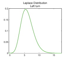
Figure 3: (a), (b) and (c) represent the Laplace distributions fitted on lateral acceleration values for right turns, straight forward and left turns respectively.

We compare four different values of $\gamma_{t}$ for the estimation of the transition matrix. First, we set $\gamma_{t}=1/t^{\alpha}$ where $\alpha=0.9$. This value of forgetting factor satisfies the convergence conditions given by Cappé [9]. Second we use three different values of fixed $\gamma$, $0.01$, $0.002$ and $0.001$–corresponding to $R=0.9$ and $K=200,1000$ and $2400$ (which corresponds to a duration $2$ min, $10$ min, and $20$ min) in Eq. (13). Figure 4 shows the estimated diagonal elements of the transition matrices for one simulated signal. The simulated signal represents a journey on a city road, a highway and then back to a city road and again highway over $10^{5}$ seconds, where the sampling period is $1/2$ seconds. The straight thick black lines show the diagonal elements of true transition matrices ${\bm{Q}}_{city}$ and ${\bm{Q}}_{highway}$.

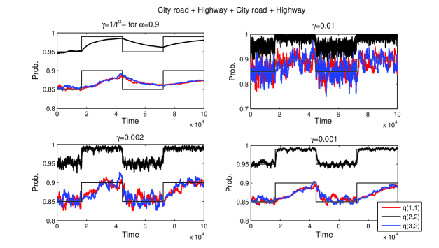
Figure 4: Diagonal elements of online estimated transition matrix, simulated signal from City road+Highway+City road+Highway, with four different values of $\gamma$. Straight thick black lines show the diagonal elements of true transition matrices ${\bm{Q}}_{city}$ and ${\bm{Q}}_{highway}$.

In Figure 4, one can see that the online algorithm with variable $\gamma$ can not follow the changes of the parameters well and that the adaption diminishes over time, as is to be expected. The fixed forgetting factor, however, seems to adapt well to the chaining environment.

Expected number of events

Here, we compute the expected number of turns. We simulate independently hundred signals in order to investigate the accuracy of the online algorithm with different forgetting factors $\gamma$. In that case, we choose as before four different values of forgetting factors, which the fixed values correspond to the weight $R=0.9$ given by the $K=200,1000$ and $2400$ latest observations in Eq. $(\ref{gam})$.

We perform 100 simulations and estimate the intensities of occurrences of turns by Eq. $(\ref{IntEvents})$:

$$\eta_{LT}=\sum_{t=1}^{T}(\pi_{t,2}\hat{q}_{t}(2,3)+\pi_{t,1}\hat{q}_{t}(1,3)),$$ (24)

$$\eta_{RT}=\sum_{t=1}^{T}(\pi_{t,2}\hat{q}_{t}(2,1)+\pi_{t,3}\hat{q}_{t}(3,1)).$$ (25)

In order to validate the results, we compute an error rate which is the difference between the estimated and observed number of turns in each simulation. The expected number of turns from the model (using ${\bm{Q}}_{city}$ and ${\bm{Q}}_{highway}$) are $\eta_{LT}=\eta_{RT}=2840$. The average number of observed left and right turns are $n_{LT}=2834$ and $n_{RT}=2836$, respectively. The average and the standard deviations of errors for 100 simulations are computed. The results are presented in Table 1. According to the average error, the forgetting factor $\gamma_{t}=0.002$ performs the best. However there is, surprisingly, only a small difference between all the fixed forgetting factors.

Table 1: The expected number of turns estimated by online algorithm and Eqs. $(\ref{countEvents_L}),(\ref{countEvents_R})$. The errors are the average of the differences between the estimated and observed number of turns.

Online algorithm
$\gamma_{t}$	$1/t^{0.9}$		$0.01$		$0.002$		$0.001$
Turns	$\eta_{LT}$	$\eta_{RT}$	$\eta_{LT}$	$\eta_{RT}$	$\eta_{LT}$	$\eta_{RT}$	$\eta_{LT}$	$\eta_{RT}$
Mean  Est.	3236	3241	2928	2932	2882	2886	2920	2924
Mean Error	402.48	405.30	94.40	96.46	48.45	49.93	86.84	88.68
Std Error	28.45	33.78	15.41	15.79	16.61	17.77	20.65	21.43

In our previous work, an HMM combined with a Viterbi algorithm [37] has been used to identify the driving events. The Viterbi algorithm gives a reconstructed sequence of events which maximizes the conditional probability of the observation sequence. In that approach, all data has to be used to estimate the driving events and is thus not suitable to on-board usage in a vehicle. However, in order to compare the previously proposed approach with the online estimation and to evaluate the frequencies of driving events, we also compute the number of turns by the Viterbi algorithm for each simulation. The counted number of turns from the Viterbi algorithm are on average $\eta_{LT}=2923$ and $\eta_{RT}=2925$. One can see that the Viterbi algorithm overestimates the number of turns.

Damage investigation

In this section we compute the damage intensity based on online estimation of transition matrix per kilometer. We use one of the simulated lateral acceleration signals in order to calculate the damage. The speed of the vehicle is considered 50 kilometers per hour and the mileage is 1000 km (for a sampling period of $1/2$ seconds). We split the signal into 1000 equally sized frames. For each frame, the expected number of turns are computed by $\Delta\eta_{k}=\eta_{k}-\eta_{k-1}$ where $\eta_{k}$ is the estimated number of turns occurring up to $k^{th}$ frame. The expected damage based on turns for each frame is calculated by:

$$\Delta d_{k}=\Delta\eta_{k}d_{k},$$

where $d_{k}$ is the expected damage per turn and calculated by means of Eqs. (18) and (22). The empirical distribution of $M_{i}$ and $m_{i}$ are used to calculate the intensity of interval crossings $\mu^{osc}(u,v)$. We use the online estimation of transition matrix ${\bm{Q}}$ with $\gamma=0.002$ to estimate the transition matrix ${\bm{P}}$ by using Eqs. (28) and (27), see Appendix A. The result for damage exponent $\beta=3$ is shown in Figure 5.  The straight thick red line shows $\Delta d_{k}({\bm{Q}}_{true})$ which is the damage intensity computed using the model transition matrices ${\bm{Q}}_{city}$ and ${\bm{Q}}_{highway}$ for city and highway respectively. We can observe the change in damage between highway and city road. As might be expected the damage intensities (per km) estimated for the city are higher than for highway, since the number of turns occurring in a city road are larger than on a highway.

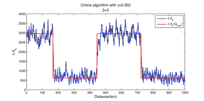
Figure 5: Damage intensity per km according to the online estimation of transition matrix with $\gamma=0.002$. The upper plot shows the results for damage exponent $\beta=3$. The straight thick red line shows $\Delta d_{k}({\bm{Q}}_{true})$ which is the damage intensity computed using model transition matrices ${\bm{Q}}_{city}$ and ${\bm{Q}}_{highway}$ for city and highway, respectively.

Further, the expected damage from the model (theoretical damage) is compared with the total damage and the damage calculated from the reduced load. One can see that the expected damage for the whole signal – based on online estimation of transition matrix– is equal to $\sum^{1000}_{k=1}\Delta d_{k}$. The total damage is calculated from the lateral acceleration signal using the rainflow method. The damage evaluated for the load (lateral acceleration), reduced load and the expected damage is compared in Table 2. The numerical integration in (18) as well as the rainflow cycle counting has been done using the WAFO (Wave Analysis for Fatigue and Oceanography) toolbox, see [8, 38].

Table 2: Comparison of damage computed for the simulated load, the corresponding reduced load and the expected damage.

Damage	Total	Reduced load	Expected
			Online with $\gamma=0.002$
$\beta=3$	$1.88\cdot 10^{6}$	$1.68\cdot 10^{6}$	$1.68\cdot 10^{6}$
$\beta=5$	$1.77\cdot 10^{8}$	$1.72\cdot 10^{8}$	$1.67\cdot 10^{8}$

Figure 5 and Table 2 demonstrate high accuracy of the proposed approach to estimate the expected damage for the studied load. Obviously this load is a realistic mathematical model of a real load. In the next section we will apply our method to estimate the steering events and compute the damage for a measured load on a VOLVO truck.

4.2 On-board logging data from Volvo

To evaluate the method on a real data set, we study field measurements coming from a Volvo Truck. We use the measured lateral acceleration signal from the CAN (Controller Area Network) bus data.

We fit the Laplace distribution for the lateral acceleration within each steering state. To estimate the Laplace distribution parameters considered, we need a training set which contains all history about the curves. We detect the events manually by looking at video recordings from the truck cabin to see what happened during the driving. The manual detections are not completely correct because of the visual errors and the low quality of videos used for the manual detection.

The online algorithms are used to count the number of left and right turns. Figure 6 shows the estimation results using online algorithm with $\gamma_{t}=0.0008\,(R=0.8,K=2000)$ for the measured signal. It is interesting to note that there is a sudden change in the driving environment after around 5000 sec.

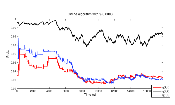
Figure 6: Diagonal elements from online estimation of transition matrix with $\gamma_{t}=0.0008$ for measured data

The expected number of left and right turns computed by online algorithm are $\eta_{LT}=228$ and $\eta_{RT}=241$ respectively.

Damage investigation

Here, we compute the damage intensity based on the model. In order to do that we split data into the frames containing $250$ seconds (approximately 4-5 km) of measurement and we compute the distance based on the average speed in each frame. Figure 7 shows the expected damage based on turns computed by $\Delta d_{k}=\Delta\eta_{k}d_{k}$ where $\Delta\eta_{k}=\eta_{k}-\eta_{k-1}$ and $n_{k}$ is the estimated number of turns occur over $k$ kilometers. Here, the results are based on the damage exponent $\beta=3$.

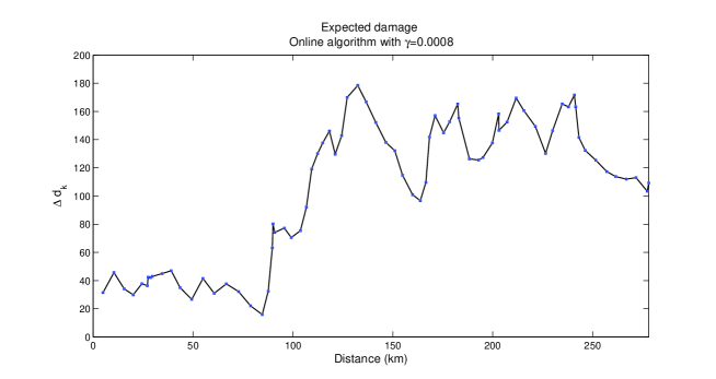
Figure 7: Damage intensity with damage exponent $\beta=3$ regarding mileage. The online estimation of transition matrix with $\gamma=0.0008$ has been used to estimate the expected damage.

The total expected damage using online estimation of transition matrix can be computed by $\sum_{k=1}\Delta d_{k}$. The damage evaluated for the load (lateral acceleration), reduced load and the expected damage is compared in Table 3. The Rayleigh distributions which have been fitted to positive and negative values of the reduced load are

$$P(M_{1}>v)=e^{-\frac{1}{2}\left(\frac{v}{2.2}\right)^{2}},\,v\geq 0,\qquad P(m_{1}<u)=e^{-\frac{1}{2}\left(\frac{u}{2.3}\right)^{2}},\,u\leq 0.$$

Table 3: Comparison of damage values computed from the measured load, the corresponding reduced load and the expected damage.

Damage	Total	Reduced load	Expected
			Online with $\gamma=0.0008$
$\beta=3$	$8.1\cdot 10^{3}$	$7.4\cdot 10^{3}$	$7.7\cdot 10^{3}$
$\beta=5$	$1.5\cdot 10^{5}$	$1.5\cdot 10^{5}$	$1.9\cdot 10^{5}$

We also compare the damage accumulation process from the model, $\sum_{k=1}\Delta d_{k}$, with the empirical accumulated damage in the signal. The expected damage based on fitted model will be called the theoretical damage. Figure 8 shows the theoretical and observed accumulated damage processes. It can be seen that the accumulated damage from the model is close to the observed damage and there are two damage rates in both theoretical and observed damage processes.

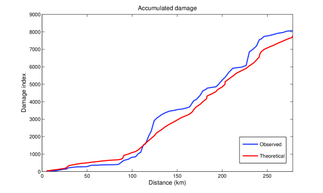
Figure 8: The theoretical and observed accumulated damage processes for damage exponent $\beta=3$. The online estimation of transition matrix with $\gamma=0.0008$ has been used to estimate the expected damage.

Results shown in Figure 8 and Table 3 demonstrate the accuracy of the proposed methodology for this measured load.

5 Conclusion

In this article, we have derived a method to estimate the number of driving events for a vehicle using the CAN data through the use of an HMM. The method uses an online EM algorithm to estimate the parameters of the HMM. The online version has three major advantages over the regular EM algorithm, making it possible to implement the method on-board a vehicle: the computational complexity of each iteration of the algorithm is $\mathcal{O}(1)$, making it a computationally tractable method; the parameters are estimated without the need to store any data; the formulation of the online algorithm allows for an adaptive parameter estimation method, using a fixed forgetting factor, so that the parameters can adapt over chaining driving environment.

The proposed estimation algorithm was validated using simulated and measured data sets. The results show that the online algorithm works well and can adapt to a chaining environment when the driving conditions are not constant over time.

Appendix A Derivation of transition matrix of driving events.

To construct the sequence $\{Z^{*}_{i}\}_{i=0}^{N}$, of driving events, let $\{t_{k}\}_{k=0}^{N}$ be the indices in $\{t:Z_{t_{k}}\neq Z_{t_{k}-1}\cap Z_{t_{k}}\neq SF\}$, then

$$Z^{*}_{k}=\begin{cases}1,&\mbox{if }Z_{t_{k}}=LT,\\ 2,&\mbox{if }Z_{t_{k}}=RT.\end{cases}$$ (26)

Assume that $Z^{*}$ has transition matrix ${\bm{P}}=(p(k,j))$. Note that the hidden process $\{Z_{t}\}_{t=0}^{T}$ in HMM has three states $"1"=\textrm{RT}$, $"2"=\textrm{SF}$ and $"3"=\textrm{LT}$. One can now derive the transition matrix ${\bm{P}}$ from the transition matrix of the HMM $\hat{{\bm{Q}}}$ as follows:

$$\hat{p}(1,1) =\frac{\hat{q}(3,2)\hat{q}(2,3)}{(1-\hat{q}(2,2))(1-\hat{q}(3,3))},$$ (27)

$$\hat{p}(2,2) =\frac{\hat{q}(1,2)\hat{q}(2,1)}{(1-\hat{q}(2,2))(1-\hat{q}(1,1))}.$$ (28)

As proof, we consider for instance the probability of going from LT to RT in $Z_{i}$ which can be computed as follows:

$$\hat{p}(1,2) =P(Z^{*}_{i}=1,Z^{*}_{i+1}=2)$$

$$=P(Z_{t_{i,start}:t_{i,stop}}=3,Z_{t_{i,stop}+1:t_{i+1,start}-1}=2,Z_{t_{i+1,start}:t_{i+1,stop}}=1)$$

$$\,\qquad\qquad\qquad\qquad+P(Z_{t_{i,start}:t_{i,stop}}=3,Z_{t_{i+1,start}:t_{i+1,stop}}=1),$$

$$=\left(\hat{q}(3,2)\left(1+\hat{q}(2,2)+\hat{q}^{2}(2,2)+...\right)\hat{q}(2,1)+\hat{q}(3,1)\right)$$

$$\,\qquad\qquad\qquad\qquad\qquad(1+\hat{q}(3,3)+\hat{q}^{2}(3,3)+...),$$

$$=\left[\frac{\hat{q}(3,2)\hat{q}(2,1)}{1-\hat{q}(2,2)}+\hat{q}(3,1)\right]\frac{1}{1-\hat{q}(3,3)}.$$

where $Z_{t_{i,start}:t_{i,stop}}$ represents the sequence of consecutive driving states $Z_{t_{i,start}},...,Z_{t_{i,stop}}$.

References

- [1] L Arvastson, H Olsson, and J Holst. Asymptotic bias in parameter estimation of ar-processes using recursive least squares with exponential forgetting. Scandinavian Journal of Statistics, 27(1):177–192, 2000.
- [2] O. Barndorff-Nielsen, J. Kent, and M. Sorensen. Normal variance-mean mixtures and z distributions. International Statistical Review, 50:145–159, 1982.
- [3] A. K. Bengtsson and I. Rychlik. Uncertainty in fatigue life prediction of structures subject to gaussian loads. Probabilistic Engineering Mechanics, 2009.
- [4] H. Berndt and K. Dietmayer. Driver intention inference with vehicle onboard sensors. In IEEE International Conference on Vehicular Electronics and Safety (ICVES), pages 102–107, Pune, 11-12 November 2009.
- [5] A. Beste, K. Dressler, H. Kötzle, W. Krüger, B. Maier, and J. Petersen. Multiaxial rainflow – a consequent continuation of Professor Tatsuo Endo’s work. In Y. Murakami, editor, The Rainflow Method in Fatigue, pages 31–40. Butterworth-Heinemann, 1992.
- [6] Bishop and Sherratt. A theoretical solution for estimation of rainflow ranges from power spectral density data. Fatigue Frac Eng Mater Struct, 13:311–326, 1990.
- [7] K. Bogsjö, K. Podgorski, and I. Rychlik. Models for road surface roughness. Vehicle System Dynamics, 50:725–747, 2012.
- [8] P. A. Brodtkorb, P. Johannesson, G. Lindgren, I. Rychlik, J. Rydén, and E. Sjö. WAFO – a Matlab toolbox for analysis of random waves and loads. In Proceedings of the 10th International Offshore and Polar Engineering conference, Seattle, volume III, pages 343–350, 2000.
- [9] O. Cappé. Online EM algorithm for hidden Markov models. Journal of Computational and Graphical Statistics, 20:3:728–749, 2011.
- [10] O. Cappé, E. Moulines, and T. Rydén, editors. Inference in Hidden Markov Models. Springer, 2005.
- [11] A. P. Dempster, N. M. Laird, and D. B. Rubin. Maximum likelihood from incomplete data via EM algorithm. Journal of the Royal Statistical Society. Series B (Methodological), 39(1):1–38, 1977.
- [12] M. Frendahl and I. Rychlik. Rainflow analysis - Markov method. Int. J. Fatigue, 15:265–272, 1993.
- [13] Sylvia Frühwirth-Schnatter. Finite Mixture and Markov Switching Models. Springer, 2006.
- [14] P. Johannesson. Rainflow cycles for switching processes with Markov structure. Probability in the Engineering and Informational Sciences, 12:143–175, 1998.
- [15] P. Johannesson. Rainflow Analysis of Switching Markov Loads. PhD thesis, Lund Institute of Technology, 1999.
- [16] P. Johannesson and M. Speckert, editors. Guide to Load Analysis for Durability in Vehicle Engineering. Wiley:Chichester, 2013.
- [17] M. Karlsson. Load Modelling for Fatigue Assessment of Vehicles – a Statistical Approach. PhD thesis, Chalmers University of Technology, Sweden, 2007.
- [18] S. Kotz, T. Kozubowski, and K. Podgorski. The Laplace distribution and generalizations: a revisit with applications to communications, economics, engineering, and finance. Springer Science & Business Media, 2001.
- [19] S . Krenk and H. Gluver. A markov matrix for fatigue load simulation and rainflow range evaluation. Struct Saf, 6:247–258, 1989.
- [20] M. Kvanström, K. Podgórski, and I. Rychlik. Laplace moving average model for multi-axial responses in fatigue analysis of a cultivator. Probabilistic Engineering Mechanics, 34:12–25, 2013.
- [21] G. Lindgren and KB. Broberg. Cycle range distributions for gaussian processes - exact and approximate results. Extremes, 7:69–89, 2004.
- [22] Lennart Ljung and Torsten Söderström. Theory and practice of recursive identification. 1983.
- [23] R. Maghsood. A statistical approach for detecting driving events and evaluating their fatigue damage, Lic. Thesis, Chalmers University of Technology, 2014.
- [24] R. Maghsood and P. Johannesson. Detection of the curves based on lateral acceleration using hidden Markov models. Procedia Engineering, 66:425–434, 2013.
- [25] R. Maghsood, I. Rychlik, and J. Wallin. Modeling extreme loads acting on steering components using driving events. Probabilistic Engineering Mechanics, 41:13–20, 2015.
- [26] M. Matsuishi and T. Endo. Fatigue of metals subjected to varying stress. Japan Society of Mechanical Engineers, 1968. In Japanese.
- [27] M. A. Miner. Cumulative damage in fatigue. Journal of Applied Mechanics, 12:A159–A164, 1945.
- [28] D. Mitrović. Learning Driving Patterns to Support Navigation. PhD thesis, University of Canterbury, New Zealand, 2004.
- [29] D. Mitrović. Reliable method for driving events recognition. IEEE Transactions on Intelligent Transportation Systems, 6(2):198–205, 2005.
- [30] A. Palmgren. Die Lebensdauer von Kugellagern. Zeitschrift des Vereins Deutscher Ingenieure, 68:339–341, 1924. In German.
- [31] I. Rychlik. A new definition of the rainflow cycle counting method. International Journal of Fatigue, 9:119–121, 1987.
- [32] I. Rychlik. Rain flow cycle distribution for ergodic load processes. SIAM J Appl Math, 48:662–679, 1988.
- [33] I. Rychlik. Note on cycle counts in irregular loads. Fatigue & Fracture of Engineering Materials & Structures, 16:377–390, 1993.
- [34] I. Rychlik. Note on modelling of fatigue damage rates for non-Gaussian stresses. Fatigue & Fracture of Engineering Materials & Structures, 36:750–759, 2013.
- [35] I. Rychlik, G. Lindgren, and Y.K. Lin. Markov based correlations of damages in Gaussian and non-Gaussian loads. Probabilistic Engineering Mechanics, 10:103–115, 1995.
- [36] Ardalan Vahidi, Anna Stefanopoulou, and Huei Peng. Recursive least squares with forgetting for online estimation of vehicle mass and road grade: theory and experiments. Vehicle System Dynamics, 43(1):31–55, 2005.
- [37] A. J. Viterbi. Error bounds for convolutional codes and an asymptotically optimal decoding algorithm. IEEE Transactions on Information Theory, IT-13(2):260–269, 1967.
- [38] WAFO Group. WAFO – a Matlab toolbox for analysis of random waves and loads, tutorial for WAFO 2.5. Mathematical Statistics, Lund University, 2011.
-
[39]
WAFO Group.
WAFO – a Matlab Toolbox for Analysis of Random Waves and Loads,
Version 2.5, 07-Feb-2011.
Mathematical Statistics, Lund University, 2011.
Web: http://www.maths.lth.se/matstat/wafo/ (Accessed 24 January 2014). - [40] O. Zeitouni and A. Dembo. Exact filters for the estimation of the number of transitions of finite-state continuous-time Markov processes. IEEE Transactions on Information Theory, 34(4):890–893, 1988.