Disentangling regular and chaotic motion in the standard map using complex network analysis of recurrences in phase space

Abstract

Recurrence in the phase space of complex systems is a well-studied phenomenon, which has provided deep insights into the nonlinear dynamics of such systems. For dissipative systems, characteristics based on recurrence plots have recently attracted much interest for discriminating qualitatively different types of dynamics in terms of measures of complexity, dynamical invariants, or even structural characteristics of the underlying attractor’s geometry in phase space. Here, we demonstrate that the latter approach also provides a corresponding distinction between different co-existing dynamical regimes of the standard map, a paradigmatic example of a low-dimensional conservative system. Specifically, we show that the recently developed approach of recurrence network analysis provides potentially useful geometric characteristics distinguishing between regular and chaotic orbits. We find that chaotic orbits in an intermittent laminar phase (commonly referred to as sticky orbits) have a distinct geometric structure possibly differing in a subtle way from those of regular orbits, which is highlighted by different recurrence network properties obtained from relatively short time series. Thus, this approach can help discriminating regular orbits from laminar phases of chaotic ones, which presents a persistent challenge to many existing chaos detection techniques.

In recent years, complex network theory has provided many conceptual insights based on recurrence characteristics of time series from various fields, which is referred to as recurrence network analysis. While recent applications of this novel concept have been restricted almost exclusively to dissipative dynamics (i.e., the quantitative characterization of attractors), we demonstrate in this work that some of the characteristic features of recurrence networks are useful for disentangling the complex dynamics of low-dimensional conservative systems as well. In the standard map, a typical chaotic orbit can be temporarily trapped in the vicinity of the regular domains in phase space, resulting in a possibly rather long time necessary to homogeneously fill the chaotic domain – a phenomenon known as stickiness. The presence of sticky orbits (i.e., intermittent laminar phases of chaotic trajectories) presents an ongoing challenge to numerically characterizing the associated phase portraits. In this work, we demonstrate that in the standard map, the geometric organization of regular orbits as well as sticky versus filling parts of chaotic orbits in phase space can be successfully discriminated based on relatively short time series by using several recurrence network measures, including network transitivity, global clustering coefficient and average path length. This result provides the first documented finding pointing to the relevance of recurrence network analysis for studying conservative dynamical systems.

I Introduction

The importance of Poincaré’s recurrences in dynamical systems has been widely recognized  Poincaré (1890). In the last decades, considerable theoretical progress has been made regarding the dynamical characteristics of various types of complex systems. One particularly important achievement has been the introduction of a rather simple visualization technique for recurrences in phase space, the recurrence plot Eckmann et al. (1987); Marwan et al. (2007), which reduces the fundamental complexity of studying recurrences to a binary matrix representation. This conceptually simple mathematical form allows drawing upon analogies to basic concepts of nonlinear time series analysis Faure and Korn (1998); Thiel et al. (2004), information theory (statistics on binary sequences providing measures of dynamical disorder and complexity) Zbilut and Webber Jr. (1992); Marwan et al. (2002) or, more recently, complex network theory Marwan et al. (2009); Donner et al. (2010, 2011). These analogies have opened important research avenues for using different types of statistics based on recurrences, which are nowadays widely applied to time series from various fields. While most recent studies have been restricted to dissipative dynamics (i.e., the quantitative characterization of attractors), we demonstrate in this work that some of the characteristic features of recurrence networks are useful for studying conservative systems as well.

The phase space of many non-integrable Hamiltonian systems is composed of intermingled regions of regular and irregular orbits Bountis and Skokos (2012). The regular domain comprises the state vectors on both periodic and quasi-periodic trajectories, while the irregular one contains the states forming chaotic orbits. Here, a typical chaotic trajectory needs a certain time to homogeneously fill its corresponding domain in phase space. However, once a chaotic orbit gets close to a stable periodic island (i.e., the regular domain), it can be trapped in the vicinity of this domain and, hence, appear almost regular in its motion for a substantial amount of time. After this intermittent laminar phase, the orbit escapes again to the rest of the chaotic domain, eventually describing chaotic bursts across the termination of this phase. Such an intermittent, possibly long-term confinement of the trajectory close to the regular domain is commonly referred to as stickiness Karney (1983); Meiss (1992) and has been accepted as a fundamental property of many Hamiltonian systems. Among other possible scenarios Afraimovich and Zaslavsky (1998), the existence of (regular) islands-around-islands embedded in the chaotic domain is one of the mechanisms that is able to generate stickiness Meiss (1992); Zaslavsky (2002). As a particularly relevant consequence, stickiness has been demonstrated to result in anomalous transport phenomena in the phase space of Hamiltonian systems.

The most traditional way of discriminating qualitatively different types of dynamics is computing or numerically estimating the largest Lyapunov exponent $\lambda$ Ott (1993). Chaotic motion is characterized by positive $\lambda$ (in the case of conservative systems, the sum of all exponents is zero). Regular orbits, on the other hand, have zero Lyapunov exponents. In practice, finite-time Lyapunov exponents are commonly used when resorting to numerical calculations. In such cases, considerable attention has to be paid to the convergence rate of the employed method, since the proper estimation of $\lambda$ becomes extremely challenging if the observed orbit encounters a sticky phase or exhibits another type of intermittent behavior Afraimovich and Zaslavsky (1998, 2003). Recent work Kandrup et al. (1999) has proposed circumventing the corresponding problems by considering sticky and filling chaotic phases separately. This distinction can be useful for chaotic orbits that have a long sticking time Contopoulos et al. (1997) and shall also be employed throughout the remainder of this manuscript.

Beyond the concept of Lyapunov exponents, there is a vast body of methods for detecting chaos from time series Bountis and Skokos (2012). Most of these approaches make use of the transverse stability of regular orbits in contrast to the exponential divergence of initially close trajectories in the case of chaos, thereby providing heuristic simplifications of the classical Lyapunov exponent concept. As a potential alternative, in this work we further explore the potentials of recurrence plot-based methods (in particular, recurrence network analysis) for obtaining a discrimination between regular and chaotic trajectories from relatively short time series – a problem where other chaos indicators commonly experience difficulties. Corresponding studies for dissipative systems have already demonstrated the great potentials of such approaches, but have not yet been systematically extended to conservative dynamics. However, the underlying concept of recurrences in phase space is well-defined in both types of systems, so that it appears natural to apply corresponding methods to conservative systems as well. This work is intended to fill this gap.

As a paradigmatic example of an autonomous nearly-integrable system with two degrees of freedom, we restrict our attention to the standard map

$$\begin{aligned} &y_{n+1}=y_{n}+\frac{\kappa}{2\pi}\sin(2\pi x_{n}),\\ &x_{n+1}=x_{n}+y_{n+1},\end{aligned}\;\;\text{mod}\;\;1$$ (1)

with $\kappa$ denoting the system’s single control parameter, and $\mathbf{v}_{n}=(x_{n},y_{n})$ being the state vector of the system at its $n$-th iteration. This model is probably the best-studied chaotic Hamiltonian map and can be interpreted as a Poincaré section of a periodically kicked rotor Lichtenberg and Lieberman (1992); Meiss (1992).

The remainder of this paper is organized as follows: Section II briefly reviews some of the mathematical concepts of recurrence analysis, comprising different approaches that address either dynamical (Rényi entropy of second order $K_{2}$, mean recurrence time $\left<RT\right>$) or geometric characteristics (recurrence network properties). A more detailed description of all methods is provided as an Appendix. The results obtained when applying the different methods to example trajectories of the standard map are discussed in Section III, providing some particularly interesting findings based on the recurrence network approach. We use this information for discussing the corresponding potentials to discriminate between initial conditions yielding regular and chaotic orbits of the standard map, focusing on the problem of identifying and characterizing chaotic orbits in their sticky phase.

II Methods

Recurrence is a fundamental property of dynamical systems. In general, it can be conveniently analyzed by means of recurrence plots (RPs) Marwan et al. (2007) originally introduced in the seminal work of Eckmann et al. Eckmann et al. (1987) This tool provides a two-dimensional intuitive visualization of the underlying temporal recurrence patterns even for high-dimensional systems. For this purpose, one defines the recurrence matrix (RM) $R_{i,j}$ as a binary representation of whether or not pairs of observed state vectors on the same trajectory are mutually close in phase space. Given two state vectors $\mathbf{v}_{i}$ and $\mathbf{v}_{j}$ (where $i$ and $j$ denote time indices), this proximity is most commonly characterized by comparing the length of the difference vector between $\mathbf{v}_{i}$ and $\mathbf{v}_{j}$ to a prescribed maximum distance $\varepsilon$, i.e.,

$$R_{i,j}(\varepsilon)=\Theta(\varepsilon-\|\mathbf{v}_{i}-\mathbf{v}_{j}\|),$$ (2)

where $\Theta(\cdot)$ is the Heaviside function and $\|\cdot\|$ a suitable norm. In this work, we use the maximum norm for defining distances between state vectors in phase space. The properties of RPs have been intensively studied for different kinds of dynamics Marwan et al. (2007), including periodic, quasi-periodic Zou et al. (2007, 2007), chaotic, and stochastic dynamics Marwan et al. (2007).

The crucial parameter for the calculation of the RM is the recurrence threshold $\varepsilon$. There are several rules-of-thumb to select a proper value of $\varepsilon$. In many applications of RPs to time series from various fields, it was found that the recurrence patterns do not change qualitatively for a large range of $\varepsilon$, allowing for a reliable statistical analysis. Furthermore, when comparing different time series (or trajectories), there are two ways to set $\varepsilon$: (i) as a fixed value for all time series, yielding possibly different values of the recurrence rate

$$RR=\frac{2}{N(N-1)}\sum_{i>j}R_{i,j}(\varepsilon),$$ (3)

i.e., the density of non-zero entries in the RM, for different series; and (ii) as a (variable) threshold value corresponding to a fixed (desired) $RR$. Note that the method (ii) generally makes it easier to quantitatively compare the recurrence structures of different time series, since some of the characteristic statistical quantities based on the RM change systematically with an increasing $RR$. In this work, we will revisit the difference between both approaches for choosing $\varepsilon$ for a low-dimensional area-preserving map (Eq. (1)).

There is a multiplicity of approaches allowing to characterize the dynamics of a system under study based on its RM. First, it has been shown that, among other features, the length of diagonal and vertical structures in RPs can be used for defining a variety of complexity measures, which characterize properties such as the degree of determinism or laminarity of the system Zbilut and Webber Jr. (1992); Trulla et al. (1996). The resulting recurrence quantification analysis (RQA) has been widely applied for studying phenomena from various scientific disciplines Marwan et al. (2007). As demonstrated earlier Zou et al. (2007), RQA measures are able to characterize the stickiness property of chaotic orbits in Hamiltonian systems like the standard map. Therefore, in the present work, we do not include any further discussion of RQA measures to avoid repetitions.

A second approach to use recurrence properties for a quantitative characterization of the system’s dynamics makes use of the fact that several dynamical invariants, such as the Rényi entropy of second order $K_{2}$ and the correlation dimension $D_{2}$, can be reliably estimated from the RM Faure and Korn (1998); Thiel et al. (2003, 2004). Specifically, $K_{2}$ measures the average rate at which information on previous states is lost during the system’s evolution. The inverse of the entropy value thus provides a rough estimate of the time for which a reasonable prediction is possible. Accordingly, for a sequence of independent and identically distributed random numbers (white noise), $K_{2}$ tends to infinity, periodic dynamics is characterized by $K_{2}=0$, and chaotic systems yield a positive yet finite $K_{2}$, as they belong to a category between regular deterministic and stochastic systems in terms of their predictability. A quasi-periodic system shows non-trivial recurrences but low complexity Lichtenberg and Lieberman (1992), which yields $K_{2}\approx 0$. Hence, $K_{2}$ is an appropriate measure to distinguish qualitatively different behaviors of the system. For the examples considered in this paper, we use trajectories of $N=1,000$ to $5,000$ data points to estimate $K_{2}$ for each orbit, applying the algorithm proposed by Thiel et al. Thiel et al. (2004).

A third way to characterize the recurrence properties is statistically evaluating the distribution of recurrence times (RTs), which has been applied to both chaotic and stochastic systems Zaslavsky (2002); Altmann and Kantz (2005). Recurrence times refer to the time intervals after which a trajectory enters the $\varepsilon$-neighborhood of a previously visited point in phase space and are conveniently described by their empirical probability distribution $p(\tau)$. Note that $p(\tau)$ contains important information about the dynamics of the system, which can be used for detecting subtle dynamical transitions of the system under study as some characteristic parameter is varied. A periodic process shows a trivial RT distribution that yields a delta-peaked $p(\tau)$ positioned at the system’s period. A quasi-periodic process involving two incommensurate frequencies (equivalent to a linear rotation on a unit circle with an irrational frequency) displays three unique recurrence times, resulting in $p(\tau)$ being delta-peaked at the three corresponding periods. Here, the largest characteristic RT is simply the sum of the other two according to Slater’s theorem Slater (1967). This theorem has been demonstrated to provide a useful and fast tool for determining the presence of quasi-periodicity Altmann et al. (2006); Zou et al. (2007, 2007). Moreover, RT statistics have great potentials for estimating dynamical invariants (such as the information dimension $D_{1}$ and the Kolmogorov-Sinai entropy Baptista et al. (2005)) and for studying extreme events Altmann and Kantz (2005). In turn, the recurrence of extreme events in dynamical systems has been recently discussed in terms of generalized extreme value theory to define a dynamical stability indicator for Hamiltonian maps Faranda et al. (2012), an approach that is conceptually related to the focus of this study, but shall not be further discussed here. An empirical estimation of $p(\tau)$ from the RM is based on the same concept as other recurrence time statistics utilized elsewhere in the literature Chirikov and Shepelyansky (1984); Zaslavsky (2002), with a slightly different averaging over all available state vectors $\mathbf{v}_{i}$ involved (see the Appendix for details). The mean recurrence time is calculated straightforwardly as $\left<RT\right>=\int_{0}^{\infty}\tau p(\tau)d\tau$.

Finally, following a more recent approach, the RM (Eq. 2) can be re-interpreted as the adjacency matrix of a complex network, the $\varepsilon$-recurrence network (RN). In this context, each state vector $\mathbf{v}_{i}$ used in the computation of the RM is interpreted as a node of a complex network embedded in the phase space of the dynamical system under study. The quantitative analysis of RNs allows identifying transitions between different types of dynamics in a very precise way Marwan et al. (2009); Donner et al. (2011); Zou et al. (2010); Donner et al. (2011). In this paper we consider three network measures that have already been shown to distinguish between qualitatively different types of behavior in both discrete and continuous-time dissipative systems Marwan et al. (2009); Zou et al. (2010); Donges et al. (2011, 2011): global clustering coefficient $\mathcal{C}$, network transitivity $\mathcal{T}$, and average path length $\mathcal{L}$ (see the Appendix for details). Given the invariant density $\rho(x)$ of the system under study, the value of $\mathcal{T}$ can be analytically computed Donges et al. (2012) and interpreted as a generalized fractal dimension Donner et al. (2011). Specifically, high values of $\mathcal{T}$ indicate the presence of a lower-dimensional structure in phase space commonly corresponding to more regular dynamics. In contrast, the average path length behaves differently for different types of dissipative dynamical systems Marwan et al. (2009); Donner et al. (2010); Zou et al. (2010): for maps, more regular dynamics is characterized by lower values of $\mathcal{L}$, whereas the opposite applies to continuous-time systems such as dissipative chaotic oscillators.

Aspect	Measures
dynamic	$K_{2}$, $\left<RT\right>$
geometric	$\mathcal{T}$, $\mathcal{C}$, $\mathcal{L}$

Table 1: All measures based on the RM used in this study. In addition, we consider numerical estimates of the largest Lyapunov exponent $\lambda$ obtained from considerably longer trajectory segments (see text) as benchmarks.

Table 1 summarizes all measures that will be used in the following. We note that the Lyapunov exponent $\lambda$, $K_{2}$ and the RT distribution characterize time series from a dynamic perspective, whereas recurrence network analysis discloses the properties of complex systems from a geometric viewpoint. Certainly, the topological features of RNs are closely related to dynamical characteristics of the underlying system Donner et al. (2010, 2011).

III Results

III.1 Example trajectories: quasi-periodic, sticky and filling chaotic orbits

We follow the approach of Kandrup et al. Kandrup et al. (1999) and categorize the trajectories of the standard map (Eq. 1) into quasi-periodic, sticky and filling (strongly) chaotic orbits. Note that stickiness is a generic property of Hamiltonian chaos Lichtenberg and Lieberman (1992) when $t\to\infty$. However, the concept of a sticky orbit only refers to the particular time-scale during which it is stuck (i.e., an intermittent laminar phase of the chaotic orbit’s evolution). In this section, we use RN and RT characteristics to investigate whether or not it is possible to distinguish between quasi-periodic orbits and the sticky (laminar) phases of chaotic orbits from relatively short trajectory segments. Regarding other measures of RQA, we refer to our previous work Zou et al. (2007).

To illustrate our approach, we first consider three typical segments of orbits of the standard map Contopoulos et al. (1997), one of which shows the stickiness property clearly. In Fig. 1A, numerical estimates of $\lambda$ are shown for these three example segments. Here, the initially sticky chaotic trajectory segment escapes from the vicinity of the regular domain after approximately $1.65\times 10^{5}$ iterations. We call this the escape time $T_{esc}$, which is about two orders of magnitude larger than the common “observation” period in many time series analysis applications ($10^{3}$ to $10^{4}$ time steps). For better comparison, we also choose a quasi-periodic orbit together with a filling part of a chaotic one. We note that with the number of iterations being much smaller than $T_{esc}$, it is not possible to distinguish the quasi-periodic orbit from the sticky part of the chaotic trajectory based on numerical estimates of $\lambda$. Furthermore, the entropy $K_{2}$ also reveals rather little difference between the sticky segment and the quasi-periodic orbit if the number of iterations does not reach $T_{esc}$ (cf.  the red and green lines in Fig. 1B). These results demonstrate that it is necessary to look at other properties that allow for a corresponding discrimination already from time series that are considerably shorter than $T_{esc}$.

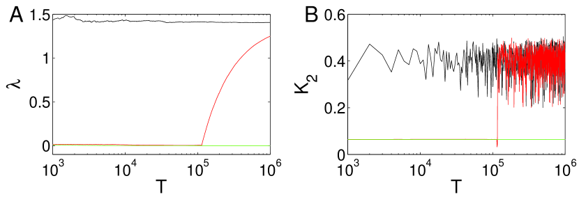
Figure 1: (color online) (A) Largest Lyapunov exponent $\lambda$ for three selected orbits ($\kappa=5$ in Eq. 1) in dependence on the considered number of iterations. The different lines represent quasi-periodic (green), sticky (red), and filling chaotic (black) orbits. (B) Rényi entropy $K_{2}$ computed for non-overlapping windows sliding along the trajectories (window length $N=1,000$).

Figure 2 shows the behavior of the three RN-based measures $\mathcal{T},\mathcal{C}$, and $\mathcal{L}$, together with the mean recurrence times $\left<RT\right>$ for the three considered trajectory segments, respectively. In all computations, we have used $RR=0.02$, maximum norm and sliding windows with $N=1,000$ subsequent state vectors taken from the respective orbits. We note that a careful statistical analysis of the probability distribution functions of all four considered measures for different types of dynamics would be required for evaluating whether or not statistically significant deviations exist among different types of trajectories. However, such a detailed analysis is beyond the scope of the present work. To this end, we emphasize that by visual inspection, one can clearly recognize that all four measures reveal distinctive differences between the considered quasi-periodic and filling chaotic orbit segments. In contrast, the sticky example orbit exhibits some distinct and quite complex behavior during different time intervals. In the latter case, the values of all considered measures quickly converge towards those of the filling chaotic orbit after the termination of the sticky phase, i.e., after the trajectory has escaped from the vicinity of the regular domain in phase space. However, a more detailed inspection reveals that based upon the RN characteristics we can distinguish three different stages: $T<T_{dec}$, $T_{dec}<T<T_{esc}$ and $T>T_{esc}$. We will discuss the meaning of $T_{dec}$ ($\approx 4\times 10^{3}$) below in some detail. The first two stages both correspond to the sticky phase of the orbit and can only be distinguished from each other by the observed values of $\mathcal{L}$, whereas the third one corresponds to the post-escape phase. The latter part of the trajectory comprises a phase of bursting behavior characterized by huge variations of all considered characteristics, which is followed by a more homogeneously filling chaotic phase interrupted by just a few short bursting intervals possibly indicating further short periods of intermittent dynamics.

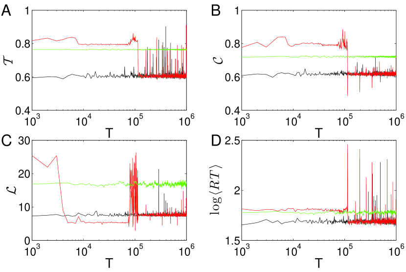
Figure 2: (color online) Recurrence characteristics for the quasi-periodic (green), sticky (red), and filling chaotic (black) orbits from Fig. 1 computed for sliding windows ($N=1,000$) over the different time series: (A) RN transitivity $\mathcal{T}$; (B) global clustering coefficient $\mathcal{C}$; (C) average path length $\mathcal{L}$; (D) logarithm of the mean recurrence time $\left<RT\right>$.

In the post-escape phase ($T>T_{esc}$), the chaotic orbit has left the vicinity of the regular domain (i.e., its intermittent laminar phase) and fills the chaotic domain of the phase space in essentially the same way as the initially filling chaotic trajectory segment. Strong fluctuations of the considered recurrence characteristics in the first part of this phase indicate the presence of chaotic bursts where the geometric structure of the orbit observed for short periods of time does not yet correspond to that of the homogeneously filling chaotic dynamics, but exhibits a strong variability. In turn, in the homogeneously filling chaotic regime, previous results for dissipative maps suggest that the three RN characteristics $\mathcal{T}$, $\mathcal{C}$ and $\mathcal{L}$ should consistently show much larger values for the regular (quasi-periodic) than for the chaotic orbits (with the exception of intermittent bursts possibly representing short periods of stickiness), which is confirmed by our numerical results.

We emphasize that intermittent bursts with strongly fluctuating RN and RT characteristics as observed in Fig. 2 are characteristic for chaotic trajectory segments and cannot be observed in the case of quasi-periodic dynamics. Hence, the presence of abrupt changes in the recurrence characteristics could serve as a criterion for identifying chaos. Notably, the latter viewpoint is not helpful when experiencing a sticky phase – or another type of intermittent behavior – during the entire period of available observations. However, the probability to encounter such a situation when choosing the initial conditions at random decreases systematically as the length of the studied trajectory segment increases.

Considering the laminar phase ($T<T_{esc}$), we find that all four characteristics show different values than for the regular (quasi-periodic) one. Notably, $\mathcal{T}$, $\mathcal{C}$ and $\left<RT\right>$ are substantially larger during the sticky phase of the chaotic trajectory in comparison with the regular orbit, while the corresponding difference is most clearly visible in the two RN characteristics (Fig. 2D). At first, this result is surprising, since $\mathcal{T}$ and $\mathcal{C}$ have an interpretation as the global and spatially averaged local (geometric) dimension of the trajectory, respectively Donner et al. (2011). Hence, one could expect that the values of both measures are smaller for a chaotic orbit (even in a sticky phase) than for a quasi-periodic one. In turn, based upon numerical studies, Tsiganis et al. Tsiganis et al. (2000) argued that “the dimension of the phase space subset on which a sticky segment is embedded does not differ from the dimension of the set on which a regular orbit lies.” According to these results, at least the correlation dimension studied in the former work allows discriminating between sticky and filling chaotic phases, but not between sticky chaotic segments and a quasi-periodic orbit.

In order to understand why we can actually observe a marked difference between sticky segments and neighboring quasi-periodic orbits, Fig. 3 highlights the geometry of the set of state vectors forming the trajectory segment during the sticky phase. We observe that as the orbits within the nearby quasi-periodic domain, in its sticky phase the chaotic orbit consists of two spatially separated parts, each of which displays two sharp kinks. For the dissipative chaotic Hénon map, it was found that such structures can spuriously induce a lower dimensionality of the system (for finite values of $\varepsilon$) due to the existence of additional closed triangles in the RN in the parts of the phase space where these kinks are located and, hence, results in a positive bias of both $\mathcal{T}$ and $\mathcal{C}$ Donner et al. (2010, 2011).

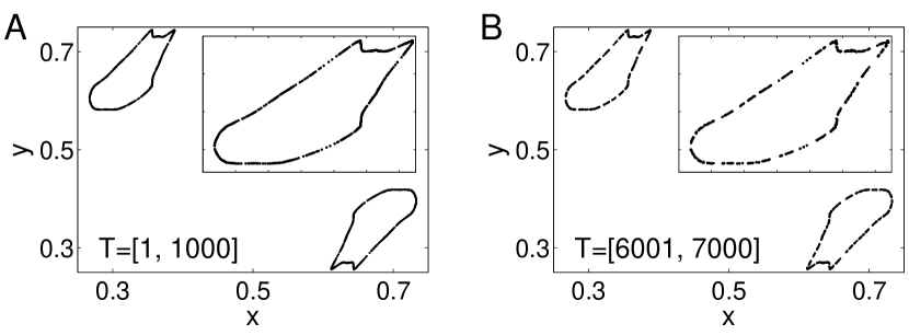
Figure 3: Phase portrait of the chaotic orbit in its sticky phase during two different periods of iterations: (A) $T=[1,1000]$, (B) $T=[6001,7000]$. Inserts show a zoom of one part of the orbit, displaying the different arrangements of the associated sets of state vectors in phase space (different distribution of gaps between neighboring state vectors).

Regarding the average path length $\mathcal{L}$, Fig. 2 shows that the RN is initially ($T<T_{dec}$) characterized by higher values for the chaotic orbit in its laminar phase in comparison with the quasi-periodic one, whereas $\mathcal{L}$ decays fastly around $T=T_{dec}$ and reaches values even below those found for the initially filling chaotic orbit for $T>T_{dec}$. The reason for this marked drop can also be identified from Fig. 3. Initially, the orbit appears more or less like a (discretely sampled) continuous curve (i.e., spatially neighboring state vectors are always separated by distances less than $\varepsilon$). In turn, at $T>T_{dec}$ distinct subsets of state vectors spanning the orbit segment get separated by increasingly large phase space regions (larger than $\varepsilon$) without state vectors. Hence, we refer to $T_{dec}$ as the RN decomposition time, which depends on the chosen value of $\varepsilon$. Consequently, the initial RN consists of mainly two mutually disconnected network components corresponding to two spatially separated parts of the regular domain in phase space (Fig. 3A), but then decomposes further into a larger number of mutually disconnected network components (which are mutually separated by more than a distance $\varepsilon$ in phase space) at $T>T_{dec}$ (cf.  the inset of Fig. 3B). Since the average path length is commonly computed over all pairs of mutually reachable nodes, it necessarily decreases if there is a transition towards more components of smaller size.

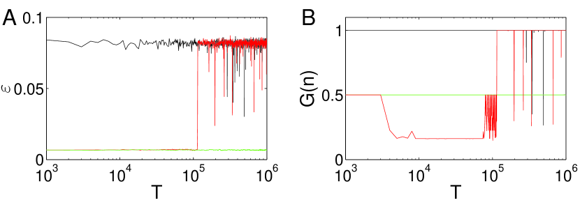
Figure 4: (A) Recurrence threshold $\varepsilon$ and (B) size of the RN’s largest component $G(n)$ for sliding windows of $N=1,000$ points along the three previously considered trajectory segments. Note that due to the presence of two spatially separated parts of the orbits, the quasi-periodic orbit (green) and the sticky phase of the chaotic orbit (red) have $G(n)\leq 0.5$, whereas the filling chaotic one (black) commonly exhibits a single component (exceptions likely correspond to short periods of stickiness or effects due to the finite sample size), i.e., $G(n)=1$.

The latter explanation is confirmed by a sharp decrease in the size of the RN’s giant component shown in Fig. 4B. We emphasize that the number of RN components $N_{c}$ would provide another suitable measure for tracing this transition. In turn, in the given situation, the RN percolation threshold $\varepsilon_{c}$ is less suited for this purpose, since the regular domain close to which the sticky orbit segment is located already consists of two spatially separated parts (as seen from the size of the largest RN component for the nearby quasi-periodic orbit exhibiting $G(n)\leq 0.5$). In contrast, the RN properties $\mathcal{L}$ and $G(n)$ unveil the mechanism how the laminar phase of the chaotic orbit is terminated: the state vectors along the chaotic trajectory get more and more concentrated in phase space, leading to the successive decomposition of the corresponding RN structure into smaller, mutually disconnected subnetworks when viewed at finite spatial resolution $\varepsilon$ for finite time windows far before the actual escape at $T=T_{esc}$. In this spirit, the decomposition of the RN provides an early indication of the loss of the stickiness property of the observed chaotic orbit. While the observations described above correspond to purely empirical findings, an in-depth analysis of the intermittent behavior of chaotic orbits of the standard map by complementary techniques like first-return maps would allow relating the reorganization of chaotic orbit segments across the escape from the sticky phase to the associated transport properties. Obviously, along with the loss of stickiness the vicinity of the invariant tori are visited more and more heterogeneously. The detailed examination of the dynamical roots of this behavior (in the context of existing results on intermittency in dynamical systems) will provide a potentially interesting topic for further studies. The same applies to the processes accompanying the trapping of a chaotic trajectory near periodic islands.

Within the framework of the present work, it would be a practically relevant question whether the observations described above are also characteristic for sticky orbits in other Hamiltonian systems. However, a detailed study of this aspect is beyond the scope of the present work. To this end, we emphasize that systematically studying $T_{dec}$ as a function of $\varepsilon$ could provide a tool for further quantitatively characterizing this transition. However, it needs to be kept in mind that the RN computed for running windows in time (i.e., consisting of a fixed number of nodes) needs to have a minimum number of edges (minimum feasible $RR$ Donges et al. (2012)) in order to allow for a proper evaluation, which sets a practical lower bound to $\varepsilon$.

Regarding the numerical results described above, it only remains to be explained why the average path length $\mathcal{L}$ initially shows larger values during the sticky phase of the chaotic trajectory segment than for the quasi-periodic orbit. Given that the recurrence threshold $\varepsilon$ is almost the same for both orbits during the full period of stickiness (cf. Fig. 4A), we relate this to the fact that (unlike for dissipative maps previously studied elsewhere Donner et al. (2010, 2011)) both the regular (quasi-periodic) orbit and the sticky phase of the chaotic one appear (up to the spatial resolution $\varepsilon$) to correspond to subsets of state vectors that exhibit no gaps larger than $\varepsilon$ in phase space (i.e., there exist relatively long paths in the RN connecting state vectors with a mutual distance of less than $\varepsilon$). In such a case, the behavior of $\mathcal{L}$ is mainly determined by the lengths of these paths, which can be analytically computed if the probability distribution function of the state vectors is known Donges et al. (2012). For the sticky phase of the chaotic orbit, the corresponding state vectors form an outer envelope of the quasi-periodic domain, so that the resulting larger spatial dimensions imply somewhat larger $\mathcal{L}$ in the RN.

Summarizing the results obtained so far, all four characteristics can potentially distinguish between quasi-periodic and sticky chaotic motion. In particular, for $\mathcal{T}$ and $\mathcal{C}$ (but to a smaller extend also $\left<RT\right>$), the observed values are consistent for the full period of stickiness and thus allow identifying sticky orbit segments even from relatively short time series (i.e., when the number of iterations is much lower than $T_{esc}$, e.g., $10^{3}-10^{4}$ iterations), because the geometric shapes of both types of orbits differ markedly. However, the aforementioned measures over-compensate the relative tendency one would actually expect for chaotic trajectories when compared to quasi-periodic ones. The latter observation is due to the stronger “kinkiness” of the sticky orbits. We will re-examine this feature below in order to address the question whether it can be exploited for automatically discriminating between quasi-periodic and sticky chaotic trajectory segments.

III.2 Full phase space

Based on the results for the three example trajectories described in Section III.1, we now turn to a characterization of the full phase space regarding different types of dynamics. For this purpose, we start with 500 initial conditions distributed randomly within the domain of definition of the standard map, $(x,y)\in[0,1]\times[0,1]$. Here, we use the canonical parameter value of $\kappa=1.4$ in Eq. 1. All trajectories are computed for $5000$ time steps. Note that for conservative dynamics we do not have transients in the sense of dissipative dynamics where an attractor needs to be approached first. This is an advantage in comparison to numerical studies of dissipative systems. Hence, the state vectors at all iterations can be further taken into account.

For the ease of comparison, Fig. 5A displays the phase space of the standard map, where a sample of state vectors of the system is colored according to the largest Lyapunov exponent $\lambda$ of the orbit traversing each corresponding point in phase space. As expected, we observe a significant difference between the chaotic domain with positive $\lambda>0$ and the regular domain with $\lambda\approx 0$. Note that for numerically approximating $\lambda$ (but not the characteristics estimated from the RM), we have used much longer trajectories with $N=2\times 10^{5}$ points, since the $N=5,000$ iterations considered in the following for computing the recurrence-based characteristics are often not sufficient for obtaining stable estimates of $\lambda$.

The resulting pattern of $K_{2}$ estimated from the RM is shown in Fig. 5B. Regarding our “experimental” setting, we emphasize that 5000 iterations often do not guarantee that all sticky orbits can leave the vicinity of the quasi-periodic areas in phase space and, hence, that a single chaotic trajectory segment can fully cover the chaotic domain. Therefore the considered trajectory length of $N=5,000$ state vectors seems to be insufficient to reliably estimate $K_{2}$, since the scaling region used for estimation Thiel et al. (2004) can eventually get blurred by short diagonal lines. This relatively short time series length explains that the numerical results of Fig. 5B do not show convincingly the theoretical relationship that $K_{2}$ is a lower bound of the sum of positive Lyapunov exponents of the system Ott (1993). However, our ensemble of 500 random initial conditions is found to be sufficient to provide a rough map of the phase space (distinguishing qualitatively different types of dynamics and highlighting domains with temporary stickiness of chaotic orbits) as shown below. Taken together, quasi-periodic orbits and chaotic trajectories in their sticky phases cannot be reliably distinguished by $K_{2}$ in the considered analysis setting.

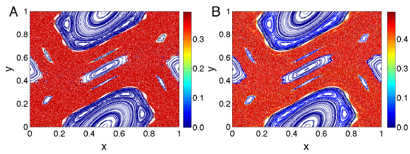
Figure 5: (color online) Phase space of the standard map (Eq. (1)) characterized by (A) the largest Lyapunov exponent $\lambda$ and (B) $K_{2}$ estimated from the RM.

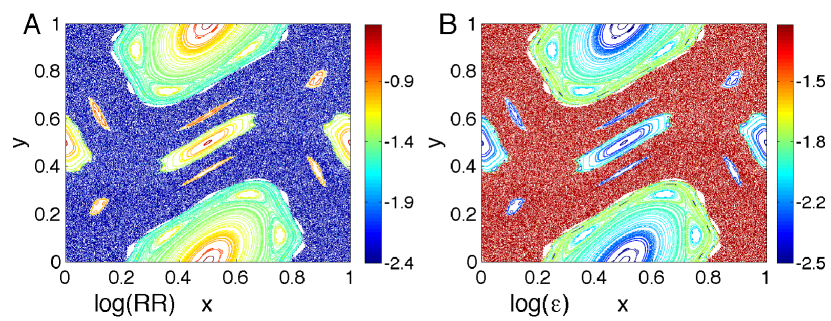
Figure 6: (color online) Same phase space as in Fig. 5, but highlighting the two different ways to choose the recurrence threshold $\varepsilon$. (A) $RR$ for a fixed threshold $\varepsilon=0.03$, (B) $\varepsilon$ for a fixed $RR=0.02$.

As discussed in detail in Section II, there are two main strategies for selecting the threshold $\varepsilon$. While the estimation of $K_{2}$ (Fig. 5B) from the RM does not distinguish between both approaches (since it uses a scaling relationship emerging as $\varepsilon$ is varied), the results for the other four characteristics depend on whether $\varepsilon$ or $RR$ is fixed. Figure 6 illustrates the mutual dependence between $\varepsilon$ and $RR$, thereby extending upon earlier results for a single orbit previously reported for dissipative chaotic systems Donner et al. (2010). Note that for Hamiltonian systems, domains covered by periodic, quasi-periodic and chaotic orbits can have intrinsically different sizes, hence, distances along such orbits are commonly not comparable. Hence, using the same $\varepsilon$ can lead to very different $RR$ (Fig. 6B).

When aiming for a quantitative comparability of RN characteristics (which can depend on $RR$), we suggest to adaptively choose $\varepsilon$ such that the $RR$ has the same fixed value (Fig. 6B). In turn, since regular and (even sticky) chaotic orbits can have considerably different spatial dimensions, it is of potential interest to also consider a setting with $\varepsilon$ being globally fixed (see Fig. 6A for the resulting behavior of $RR$). The corresponding results for the three RN measures as well as $\left<RT\right>$ for both settings are shown in Figs. 7 and 8, respectively.

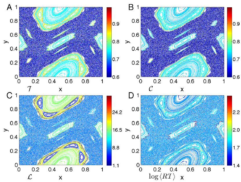
Figure 7: (color online) Same phase space as in Fig. 5, but characterized by recurrence statistics for the standard map using fixed $RR=0.02$. (A) $\mathcal{T}$, (B) $\mathcal{C}$, (C) $\mathcal{L}$, and (D) $\left<RT\right>$.

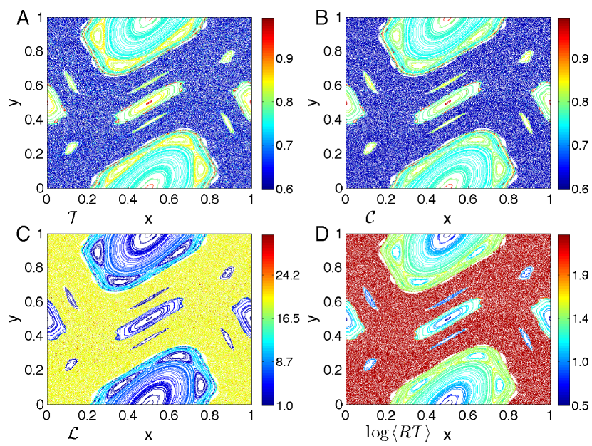
Figure 8: (color online) Same phase space as in Fig. 7 for a fixed $\varepsilon=0.03$.

The overall structure of the phase space with its intermingled regular and chaotic orbits is captured by both dynamic ($K_{2}$ and $RT$) and geometric measures (e.g., $\mathcal{T}$ and other RN characteristics), as shown in Figs. 7 and 8. Specifically, quasi-periodic trajectories are characterized by larger values of network transitivity $\mathcal{T}$, while filling chaotic ones have smaller $\mathcal{T}$. The same applies to $\mathcal{C}$. Regarding both properties, the obtained picture is consistent for the two settings with fixed $RR$ and fixed $\varepsilon$, respectively. For $\left<RT\right>$, the pattern is only conclusive for fixed $\varepsilon$, where the mean recurrence times are considerably larger in the filling chaotic case than for regular orbits (as it is the case for the RN average path length $\mathcal{L}$), which is expected since the chaotic domain is larger than the regular one. Specifically, while a chaotic orbit can fill the complete domain (as $t\to\infty$), regular ones are distinct and mutually nested, which results in different values of $\left<RT\right>$ and $\mathcal{L}$ for the latter which (for fixed $\varepsilon$) depend clearly on the size of the orbit. In turn, when fixing $RR$ the effect of different spatial distances on the estimated recurrence times and RN average path lengths is essentially removed (Fig. 7C,D).

Turning back to the original question of whether or not it is possible to distinguish chaotic trajectories in their sticky phase from quasi-periodic orbits, our results indicate that in agreement with the findings for the three example trajectories in Section III.A, the RN transitivity $\mathcal{T}$ obtained with a fixed $RR$ is a promising candidate measure. Notably, the sticky chaotic orbit segments are organized in phase space like envelopes of the islands-around-islands (i.e., a period-$n$ orbit surrounded by islands of high periods). As Fig. 9 indicates, these envelopes are in fact characterized by elevated values of $\mathcal{T}$ clearly above those found for the orbits within the regular domains ($\mathcal{T}=0.75$ – as expected for one-dimensional curves Donner et al. (2011) — in the middle of these domains and $\mathcal{T}\approx 0.8$ inside the quasi-periodic island chains), while many initial conditions close to the quasi-periodic orbits (but not belonging to them) lead to finite-time trajectory segments with $\mathcal{T}\sim 0.85\dots 0.9$ and even above due to the kinky geometry shown in Fig. 3, which is consistent with previous findings for dissipative maps Donner et al. (2010, 2011).

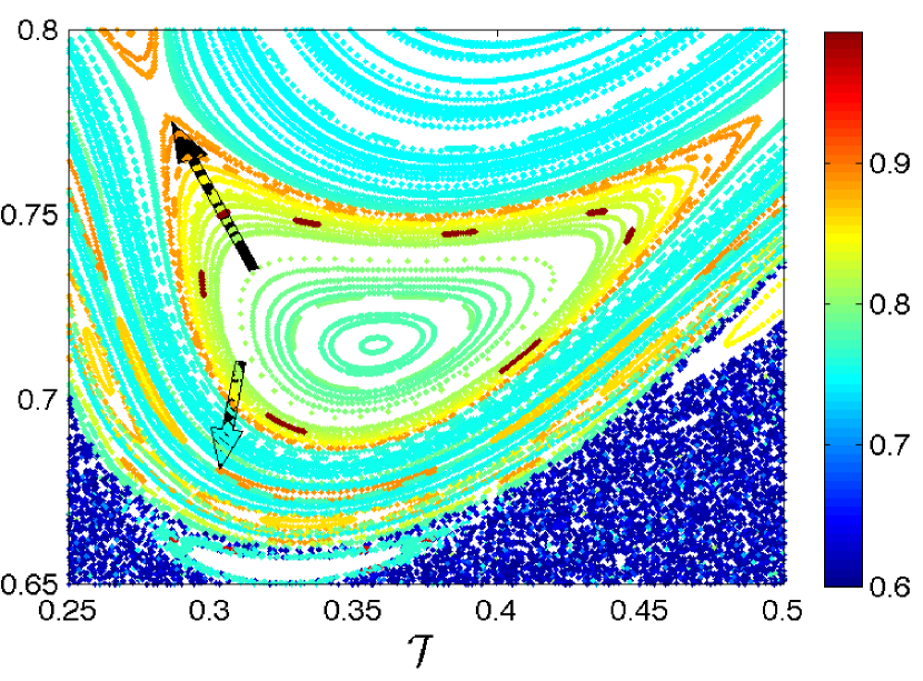
Figure 9: (color online) Zoom into Fig. 7A displaying the values of $\mathcal{T}$ at the interface between regular and chaotic domains. Black arrows indicate chaotic areas with increased transitivity values.

Following the ideas presented in our previous work on dissipative systems Zou et al. (2010), one could in principle assess the quality of a classification obtained by the approach presented above in a more rigorous statistical framework with the help of the largest Lyapunov exponent $\lambda$. However, such an assessment of the discriminatory power of different measures becomes both numerically and conceptually more challenging than for the problem of distinguishing periodic and chaotic orbits in the parameter space of dissipative nonlinear oscillators as previously studied Zou et al. (2010) for different reasons: (i) there are periodic, quasi-periodic and chaotic trajectories (i.e., three qualitatively different types of orbits) intermingled in phase space; (ii) there is no unique residence time scale for chaotic orbits to stay in an intermittent laminar phase corresponding to stickiness; and (iii) technically, the assessment is more appropriate for investigating the parameter space of complex systems Zou et al. (2010) than for exploring the phase space with coexisting domains of qualitatively different dynamics as done as in Figs. 7 and 8. The statistical analysis would hence yield results that are specific to the particular choices of the length of time series and initial conditions.

IV Conclusions

We have presented a numerical case study demonstrating that recurrence-based methods in general, and recurrence networks in particular, can be useful for disentangling different dynamical regimes not only in dissipative, but also in conservative dynamical systems. Specifically, we have shown that the geometric properties of regular (i.e., periodic and quasi-periodic) orbits of the standard map as captured by recurrence networks clearly differ from such of (filling) segments of chaotic orbits that do not exhibit intermittent periods of stickiness close to the domain of regular solutions. While in the latter case, many existing approaches can fail to unambiguously discriminate between quasi-periodic and sticky chaotic dynamics, recurrence network characteristics provide indicators for the presence of chaos even in such rather complex situations. The transition phase between laminar (sticky) and homogeneously filling chaotic dynamics has not been explicitly studied, but presents an interesting subject to be further investigated. In general, one has to note that sticky and filling chaotic dynamics can correspond to different phases of the same chaotic orbit (the durations of which can show a considerably wide distribution). Thus, making a distinction between both appearances is only reasonable for specified periods of observation of the system under study.

It is important to emphasize that the proposed application of recurrence network analysis to conservative systems has been successful already for relatively short trajectory segments (e.g., $N=1,000$ or $5,000$ points). Although this study has considered only the paradigmatic and best-studied example of a discrete-time two-dimensional Hamiltonian system exhibiting co-existence between regular orbits and chaos (the Chirikov standard map), it is expected that similar results can be obtained for other Hamiltonian maps with a chaotic regime, such as a four-dimensional version of the standard map consisting of two coupled classical standard maps Freistetter (2000), Zaslavsky’s stochastic web map Zaslavsky (1998), Meiss’ quadratic map Meiss (1986), or even continuous-time Hamiltonian system like the Hénon-Heiles system Hénon and Heiles (1964); Zou et al. (2007). A continuation of this study taking such different systems into account will be subject of our future work.

The aim of the present study was to initially explore the general potentials of recurrence network analysis for applications to conservative systems. We did neither undertake an exhaustive quantitative comparison between different recurrence-based techniques, nor between recurrence-based approaches and classical chaos indicators based on the idea of exponential transverse motion in phase space Gottwald and Skokos (2014); Bountis and Skokos (2012) or established tests for the presence of chaos like the 0-1 test Gottwald and Melbourne (2004). However, a corresponding in-depth investigation should be a subject of future research as well, including a systematic study of the effects of the available time series length on the obtained estimates.

In order to further support the applicability of the proposed approach, a detailed performance assessment of different methods would be desirable. For such an assessment, two criteria appear of special relevance:

On the one hand, the classification accuracy needs to be addressed. Notably, a corresponding investigation would require considerable numerical efforts, since the exact location of the chaotic domains cannot be computed analytically for the standard map, but needs to be evaluated by some benchmark technique. For this purpose, the standard reference would again be the largest Lyapunov exponent, the appropriate estimation of which, however, is considerably challenged by the presence of stickiness at all possible time scales (i.e., the closer an initial condition is to the boundary of the regular domain, the longer the sticking time can be expected to be). In fact, this problem affects essentially all existing classification criteria for orbits in Hamiltonian systems exhibiting stickiness phenomena.

On the other hand, convergence time should be taken into account as a second criterion, which is of particular relevance in situations where only relatively short time series are available for characterizing the nature of different orbits. Regarding the latter aspect, we emphasize that recurrence methods present a powerful methodological alternative to indicators based on transverse expansion. From the computational perspective, recurrence plot-based methods are conceptually simple and have reasonable computational demands, making them excellent candidates for applications to short experimental time series Marwan et al. (2007).

Appendix A Methodological details

In this Appendix, we provide algorithmic details on the set of complementary recurrence analysis approaches used in this paper.

A.1 Dynamical invariant $K_{2}$

We recall the techniques presented in Thiel et al. (2003, 2004) to estimate $K_{2}$ from the RM (Eq. 2) and present some remarks on the corresponding computations. $K_{2}$ can be estimated from the cumulative distribution of diagonal lines $P^{c}_{\varepsilon}(l)$ in the RP Thiel et al. (2003). Specifically, the probability of finding a diagonal line of at least length $l$ in the RP of a chaotic map is given by

$$P^{c}_{\varepsilon}(l)\sim\varepsilon^{D_{2}}\exp({-K_{2}(\varepsilon)l)}.$$ (4)

Therefore, if we represent $P^{c}_{\varepsilon}(l)$ in a logarithmic scale versus $l$, we should obtain a straight line with slope $-K_{2}(\varepsilon)$ for large $l$. This slope is independent of $\varepsilon$ for a deterministic chaotic system, while linearly dependent on $\varepsilon$ for random processes. Thus, $K_{2}$ can be estimated from RPs provided the length of time series covers the underlying system in the (sampled) phase space sufficiently well. This method has been successfully applied to characterize fluid dynamics in different regimes Thiel et al. (2004), to study the stability of extrasolar planetary systems Asghari et al. (2004), and to divide the parameter space of a mechanical oscillator system into different regimes Zou et al. (2006).

One important advantage of the RP-based estimator of $K_{2}$ (Eq. 4) is that it is independent of the choice of the parameters for a possibly necessary embedding, which can be important when studying real-world observational time series.

A.2 Recurrence time statistics from RM

The detailed steps to estimate the RT distribution $p(\tau)$ from the RM are as follows:

RTs can be identified as the lengths of non-interrupted vertical (or horizontal, since the RM is symmetric) “white lines” that do not contain any recurrence (i.e., no pair of mutually close state vectors). More precisely, such a white line of length $\tau$ starts at the position $(i,j)$ in the RP if Thiel et al. (2003)

$$R_{i,j+m}=\begin{cases}1&\text{if}\;m=-1,\\ 0&\text{for}\;m\in\{0,\ldots,\tau-1\},\\ 1&\text{if}\;m=\tau.\end{cases}$$ (5)

This means that for all times $k=j-1,\ldots,j+\tau$, the observed state vectors $\mathbf{v}_{k}$ are compared with $\mathbf{v}_{i}$. The structure given by Eq. (5) can be interpreted as follows: At time $k=j-1$, the trajectory falls into an $\varepsilon$-neighborhood of $\mathbf{v}_{i}$. Then, for $k=j,\ldots,j+\tau-1$, it moves further away from $\mathbf{v}_{i}$ than a distance $\varepsilon$, until it returns to the $\varepsilon$-neighborhood of $\mathbf{v}_{i}$ again at $k=j+\tau$. Hence, given a uniform sampling of the trajectory in the time domain, the length $\tau$ of the resulting white line in the corresponding RP is proportional to the time that the trajectory needs to return $\varepsilon$-close to $\mathbf{v}_{i}$. Going beyond the concept of first-return times, the ensemble of all recurrences to the $\varepsilon$-neighborhood of $\mathbf{v}_{i}$ induces a RT distribution for this specific point. Combining this information for all available points $\mathbf{v}_{i}$ in a given time series (i.e., considering the lengths of all white lines in the RP), one obtains the RT distribution $p(\tau)$ associated with the observed (sampled) trajectory segment in phase space. Hence, the length distribution $p(l)$ of white vertical lines $l$ in the RM not containing any recurrent pair of observed state vectors provides an empirical estimate of the distribution of RTs on the considered orbit.

A.3 Recurrence network analysis

Recently, the idea of transforming a time series into complex network representations has emerged in the scientific literature, providing new alternatives for studying basic properties of time series from a complex network perspective Zhang and Small (2006); Xu et al. (2008); Lacasa et al. (2008); Marwan et al. (2009); Donner et al. (2010, 2011). Among other corresponding approaches, the RM (Eq. 2) can be re-interpreted as the adjacency matrix of the so-called $\varepsilon$-recurrence network (RN).

In order to construct the RN, we re-consider the recurrence matrix $R_{i,j}$, the main diagonal of which is removed for convenience, as the adjacency matrix $A_{i,j}$ of an undirected complex network associated with the recorded trajectory, i.e.,

$$A_{i,j}=R_{i,j}(\varepsilon)-\delta_{i,j},$$ (6)

where $\delta_{i,j}$ is the Kronecker delta. The nodes of this network are given by the individual sampled state vectors on the trajectory, whereas the connectivity is established according to their mutual closeness in phase space. This definition provides a generic way for analyzing phase space properties of complex systems in terms of RN topology Donner et al. (2010, 2011). However, since this topology is invariant under permutations of the order of nodes, the statistical properties of RNs do not specifically capture the system’s dynamics, but its geometric structure based on an appropriate sampling. We emphasize that a single finite-time trajectory does not necessarily represent the typical long-term behavior of the underlying system. Hence, the resulting network properties can depend – among others – on the length $N$ of the considered time series (i.e., the network size), the probability distribution of the data, embedding Donner et al. (2010), sampling Facchini and Kantz (2007); Donner et al. (2011), etc.

Although they primarily describe geometric aspects, the topological features of RNs are closely related to dynamical characteristics of the underlying system Donner et al. (2010, 2011). In dissipative chaotic model systems (e.g., Rössler and Lorenz systems), both local and global network properties have already been studied in great detail Donner et al. (2011).

In this paper, we consider the following three characteristics Newman (2003); Boccaletti et al. (2006) as potential candidates for discriminatory statistics:

1. the average path length $\mathcal{L}$, which quantifies the average geodesic (graph) distance $l_{i,j}$ between all pairs of nodes $(i,j)$,

   $$\mathcal{L}=\left<l_{i,j}\right>=\frac{2}{N(N-1)}\sum_{i<j}{l_{i,j}},$$ (7)

   where $l_{i,j}$ is the minimum number of edges separating two nodes $i$ and $j$;

2. the global clustering coefficient $\mathcal{C}$ Watts and Strogatz (1998), which gives the arithmetic mean of the local clustering coefficients $\mathcal{C}_{i}$ (i.e., the fraction of nodes connected with a node $i$ that are pairwise connected themselves) taken over all $i$,

   $$\mathcal{C}=\frac{1}{N}\sum_{i=1}^{N}\mathcal{C}_{i}$$ (8)

   with

   $$\quad\mathcal{C}_{i}=\frac{\sum_{j,k;i\neq j\neq k}A_{i,j}A_{i,k}A_{j,k}}{\sum_{j,k;i\neq j\neq k}A_{i,j}A_{i,k}};$$ (9)

3. network transitivity $\mathcal{T}$ Barrat and Weigt (2000); Newman (2001), which is closely related to $\mathcal{C}$ (but gives less weight to poorly connected nodes Donner et al. (2011)) and globally characterizes the linkage relationships among triples of nodes in a complex network (i.e., the probability of a third edge within a set of three nodes given that the two other edges are already known to exist),

   $$\mathcal{T}=\frac{3\ N_{\Delta}}{N_{3}}=\frac{\sum_{i,j,k;i\neq j\neq k}A_{i,j}A_{i,k}A_{j,k}}{\sum_{i,j,k;i\neq j\neq k}A_{i,j}A_{i,k}},$$ (10)

   where $N_{\Delta}$ is the number of triangles in the network and $N_{3}$ is the number of connected triples. Note that $\mathcal{T}$ is sometimes referred to as the (Barrat-Weigt) global clustering coefficient, often also denoted as $\mathcal{C}$, e.g., in ref. Zou et al. (2010). In order to avoid confusion, in this work we prefer to discuss both measures separately.

We emphasize that further network measures (e.g., local betweenness centrality $b_{v}$ and global assortativity coefficient $\mathcal{R}$) have also been shown to discriminate between different types of dynamics in dissipative systems Marwan et al. (2009); Donner et al. (2010); Zou et al. (2010), but are not considered in this work for brevity.

References

- Poincaré (1890) H. Poincaré, “Sur la problème des trois corps et les équations de la dynamique,” Acta Mathematica, 13, A3–A270 (1890).
- Eckmann et al. (1987) J.-P. Eckmann, S. O. Kamphorst, and D. Ruelle, “Recurrence plots of dynamical systems,” Europhys. Lett., 4, 973–977 (1987).
- Marwan et al. (2007) N. Marwan, M. C. Romano, M. Thiel, and J. Kurths, “Recurrence plots for the analysis of complex systems,” Phys. Rep., 438, 237–329 (2007).
- Faure and Korn (1998) P. Faure and H. Korn, “A new method to estimate the Kolmogorov entropy from recurrence plots: its application to neuronal signals,” Physica D, 122, 265–279 (1998).
- Thiel et al. (2004) M. Thiel, M. Romano, P. Read, and J. Kurths, “Estimation of dynamical invariants without embedding by recurrence plots,” Chaos, 14, 234–243 (2004a).
- Zbilut and Webber Jr. (1992) J. P. Zbilut and C. L. Webber Jr., “Embeddings and delays as derived from quantification of recurrence plots,” Physics Letters A, 171, 199–203 (1992).
- Marwan et al. (2002) N. Marwan, N. Wessel, U. Meyerfeldt, A. Schirdewan, and J. Kurths, “Recurrence plot based measures of complexity and its application to heart rate variability data,” Phys. Rev. E, 66, 026702 (2002).
- Marwan et al. (2009) N. Marwan, J. F. Donges, Y. Zou, R. V. Donner, and J. Kurths, “Complex network approach for recurrence analysis of time series,” Phys. Lett. A, 373, 4246–4254 (2009).
- Donner et al. (2010) R. V. Donner, Y. Zou, J. F. Donges, N. Marwan, and J. Kurths, “Recurrence networks – A novel paradigm for nonlinear time series analysis,” New J. Phys., 12, 033025 (2010a).
- Donner et al. (2011) R. V. Donner, M. Small, J. F. Donges, N. Marwan, Y. Zou, R. Xiang, and J. Kurths, “Recurrence-based time series analysis by means of complex network methods,” Int. J. Bifurcation Chaos, 21, 1019–1046 (2011a).
- Karney (1983) C. Karney, “Long-time correlations in the stochastic regime,” Physica D, 8, 360–380 (1983).
- Lichtenberg and Lieberman (1992) A. Lichtenberg and M. Lieberman, Regular and Chaotic Dynamics, 2nd ed. (Springer, Berlin, 1992).
- Meiss (1992) J. Meiss, “Symplectic maps, variational principles, and transport,” Rev. Mod. Phys, 64, 795–848 (1992).
- Bountis and Skokos (2012) T. C. Bountis and C. Skokos, Complex Hamiltonian Dynamics (Springer, Berlin/Heidelberg, 2012).
- Afraimovich and Zaslavsky (1998) V. Afraimovich and G. Zaslavsky, “Sticky orbits of chaotic Hamiltonian dynamics,” in Chaos, Kinetics and Nonlinear Dynamics in Fluids and Plasmas, Lecture Notes in Physics, Vol. 511, edited by S. Benkadda and G. Zaslavsky (Springer Berlin Heidelberg, 1998) pp. 59–82.
- Zaslavsky (2002) G. Zaslavsky, “Chaos, fractional kinetics, and anomalous transport,” Phys. Rep., 371, 461–580 (2002).
- Ott (1993) E. Ott, Chaos in Dynamical Systems (Cambridge University Press, 1993).
- Afraimovich and Zaslavsky (2003) V. Afraimovich and G. M. Zaslavsky, “Spacetime complexity in Hamiltonian dynamics,” Chaos, 13, 519–532 (2003).
- Kandrup et al. (1999) H. Kandrup, C. Siopis, G. Contopoulos, and R. Dvorak, “Diffusion and scaling in escapes from two degrees of freedom Hamiltonian systems,” Chaos, 9, 381–392 (1999).
- Contopoulos et al. (1997) G. Contopoulos, N. Voglis, and R. Dvorak, “Transition spectra of dynamical systems,” Cel. Mech. Dyn. Astron., 67, 293–317 (1997).
- Zou et al. (2007) Y. Zou, D. Pazó, M. Thiel, M. Romano, and J. Kurths, “Distinguishing quasiperiodic dynamics from chaos in short-time series,” Phys. Rev. E, 76, 016210 (2007a).
- Zou et al. (2007) Y. Zou, M. Thiel, M. Romano, and J. Kurths, “Characterization of stickiness by means of recurrence,” Chaos, 17, 043101 (2007b).
- Trulla et al. (1996) L. L. Trulla, A. Giuliani, J. P. Zbilut, and C. L. Webber Jr., “Recurrence quantification analysis of the logistic equation with transients,” Physics Letters A, 223, 255–260 (1996).
- Thiel et al. (2003) M. Thiel, M. Romano, and J. Kurths, “Analytical description of recurrence plots of white noise and chaotic processes,” Appl. Nonlin. Dyn., 11, 20–29 (2003).
- Altmann and Kantz (2005) E. G. Altmann and H. Kantz, “Recurrence time analysis, long-term correlations, and extreme events,” Phys. Rev. E, 71, 56106 (2005).
- Slater (1967) N. Slater, “Gaps and steps for the sequence mod 1,” Proc. Cambridge Philos. Soc., 63, 1115–1123 (1967).
- Altmann et al. (2006) E. G. Altmann, G. Cristadoro, and D. Pazó, “Nontwist non-Hamiltonian systems,” Phys. Rev. E, 73, 056201 (2006).
- Baptista et al. (2005) M. Baptista, S. Kraut, and C. Grebogi, “Poincaré recurrence and measure of hyperbolic and nonhyperbolic chaotic attractors,” Phys. Rev. Lett., 95, 094101 (2005).
- Faranda et al. (2012) D. Faranda, V. Lucarini, G. Turchetti, and S. Vaienti, “Generalized extreme value distribution parameters as dynamical indicators of stability,” Int. J. Bifurcation Chaos, 22, 1250276 (2012).
- Chirikov and Shepelyansky (1984) B. V. Chirikov and D. L. Shepelyansky, “Correlation properties of dynamical chaos in Hamiltonian systems,” Physica D, 13, 395–400 (1984).
- Zou et al. (2010) Y. Zou, R. V. Donner, J. F. Donges, N. Marwan, and J. Kurths, “Identifying shrimps in continuous dynamical systems using recurrence-based methods,” Chaos, 20, 043130 (2010).
- Donner et al. (2011) R. V. Donner, J. Heitzig, J. F. Donges, Y. Zou, N. Marwan, and J. Kurths, “The geometry of chaotic dynamics – a complex network perspective,” Eur. Phys. J. B, 84, 653–672 (2011b).
- Donges et al. (2011) J. F. Donges, R. V. Donner, K. Rehfeld, N. Marwan, M. H. Trauth, and J. Kurths, “Identification of dynamical transitions in marine palaeoclimate records by recurrence network analysis,” Nonlin. Proc. Geophys., 18, 545–562 (2011a).
- Donges et al. (2011) J. F. Donges, R. V. Donner, M. H. Trauth, N. Marwan, H. J. Schellnhuber, and J. Kurths, “Nonlinear detection of paleoclimate-variability transitions possibly related to human evolution,” Proc. Natl. Acad. Sci. USA, 108, 20422–20427 (2011b).
- Donges et al. (2012) J. F. Donges, J. Heitzig, R. V. Donner, and J. Kurths, “Analytical framework for recurrence network analysis of time series,” Phys. Rev. E, 85, 046105 (2012).
- Tsiganis et al. (2000) K. Tsiganis, A. Anastasiadis, and H. Varvoglis, “Dimensionality differences between sticky and non-sticky chaotic trajectory segments in a 3D Hamiltonian system,” Chaos, Solitons and Fractals, 13, 2281-2292 (2000).
- Thiel et al. (2004) M. Thiel, M. Romano, P. Read, and J. Kurths, “Estimation of dynamical invariants without embedding by recurrence plots,” Chaos, 14, 234–243 (2004b).
- Donner et al. (2010) R. V. Donner, Y. Zou, J. F. Donges, N. Marwan, and J. Kurths, “Ambiguities in recurrence-based complex network representations of time series,” Phys. Rev. E, 81, 015101(R) (2010b).
- Freistetter (2000) F. Freistetter, “Fractal dimensions as chaos indicators,” Cel. Mech. Dyn. Astron., 78, 211–225 (2000).
- Zaslavsky (1998) G. Zaslavsky, Physics of Chaos in Hamiltonian Systems (Imperial College Press, London, 1998).
- Meiss (1986) J. D. Meiss, “Class renormalization: Islands around islands,” Phys. Rev. A, 34, 2375–2383 (1986).
- Hénon and Heiles (1964) M. Hénon and C. Heiles, “The applicability of the third integral of motion: some numerical experiments,” Astronom. J., 69, 73–79 (1964).
- Gottwald and Skokos (2014) G. A. Gottwald and C. Skokos, “Preface to the focus issue: Chaos detection methods and predictability,” Chaos, 24, 024201 (2014).
- Asghari et al. (2004) N. Asghari, C. Broeg, L. Carone, R. Casas-Miranda, J. C. C. Palacio, I. Csillik, R. Dvorak, F. Freistetter, G. Hadjivantsides, H. Hussmann, A. Khramova, M. Khristoforova, I. Khromova, I. Kitiashivilli, S. Kozlowski, T. Laakso, T. Laczkowski, D. Lytvinenko, O. Miloni, R. Morishima, A. Moro-Martin, V. Paksyutov, A. Pal, V. Patidar, B. Pecnik, O. Peles, J. Pyo, T. Quinn, A. Rodriguez, C. Romano, E. Saikia, J. Stadel, M. Thiel, N. Todorovic, D. Veras, E. V. Neto, J. Vilagi, W. von Bloh, R. Zechner, and E. Zhuchkova, “Stability of terrestrial planets in the habitable zone of GI77A, HD72659, GI614, 47Uma and HD4208,” Astron. Astrophys., 426, 353–365 (2004).
- Zou et al. (2006) Y. Zou, M. Thiel, M. C. Romano, Q. Bi, and J. Kurths, “Shrimp structure and associated dynamics in parametrically excited oscillators,” Int. J. Bifurcation Chaos, 16, 3567–3579 (2006).
- Zhang and Small (2006) J. Zhang and M. Small, “Complex network from pseudoperiodic time series: Topology versus dynamics,” Phys. Rev. Lett., 96, 238701 (2006).
- Xu et al. (2008) X. Xu, J. Zhang, and M. Small, “Superfamily phenomena and motifs of networks induced from time series,” Proc. Natl. Acad. Sci. USA, 105, 19601–19605 (2008).
- Lacasa et al. (2008) L. Lacasa, B. Luque, F. Ballesteros, J. Luque, and J. C. Nuno, “From time series to complex networks: The visibility graph,” Proc. Natl. Acad. Sci. USA, 105, 4972–4975 (2008).
- Facchini and Kantz (2007) A. Facchini and H. Kantz, “Curved structures in recurrence plots: The role of the sampling time,” Phys. Rev. E, 75, 036215 (2007).
- Newman (2003) M. E. J. Newman, “The structure and function of complex networks,” SIAM Rev., 45, 167–256 (2003).
- Boccaletti et al. (2006) S. Boccaletti, V. Latora, Y. Moreno, M. Chavez, and D.-U. Hwang, “Complex networks: Structure and dynamics,” Phys. Rep., 424, 175–308 (2006).
- Watts and Strogatz (1998) D. J. Watts and S. H. Strogatz, “Collective dynamics of “small-world” networks,” Nature, 393, 440–442 (1998).
- Barrat and Weigt (2000) A. Barrat and M. Weigt, “On the properties of small-world network models,” Eur. Phys. J. B, 13, 547–560 (2000).
- Newman (2001) M. E. J. Newman, “Scientific collaboration networks. i. network construction and fundamental results,” Phys. Rev. E, 64, 016131 (2001).
- Gottwald and Melbourne (2004) G. A. Gottwald and I. Melbourne, “A new test for chaos in deterministic systems,” Proc. R. Soc. London A, 460, 603–611 (2004).