Point splitting renormalization of Schwinger induced current in de Sitter spacetime

Abstract

The covariant and gauge invariant calculation of the current expectation value in the homogeneous electric field in 1+3 dimensional de Sitter spacetime is shown. The result accords with previous work obtained by using adiabatic subtraction scheme. We therefore conclude the counterintuitive behaviors of the current in the infrared (IR) regime such as IR hyperconductivity and negative current are not artifacts of the renormalization scheme, but are real IR effects of the spacetime.

1 Introduction

Investigation of quantum field theory in curved spacetime background has a long history. We cannot put enough emphasis on the importance of the study in the context of cosmology [1, 2]. Inflationary background, which is approximately described by de Sitter spacetime, may be the most interesting and relevant subject (for a review of inflationary cosmology, see e.g. [3]). One of the greatest achievements in the inflationary cosmology is the prediction of the primordial perturbations which is supposed to become a seed of all the structure in the later universe. Their calculation is entirely based on quantum field theory in curved spacetime and the agreement with observations infers the correctness of the approach. Not only the scalar perturbation but also the vector and tensor perturbations can be generated from the quantum fluctuations in the inflationary universe. The cosmic microwave background (CMB) observations basically espouse the generation of the primordial scalar perturbation. The primordial tensor perturbation has also been investigated and detection of the primordial gravitational waves is awaited.

The primordial vector perturbation is usually less significant since it only has decaying modes. On the other hand, the observations of galactic/extragalactic magnetic field [4, 5, 6, 7, 8, 9, 10, 11] indicate the existence of large scale magnetic field in extragalactic scale whose origin is yet to be clarified. The inflationary magnetogenesis is a serious candidate since it may be able to produce coherent magnetic fields on large scale, especially, extragalactic scales ($\sim$Mpc). Thus it is motivated to modify the standard theory which is conformally invariant and hence no long-wave perturbations are expected so that the primordial vector perturbation can be generated during inflationary era. Among many proposed mechanisms of inflationary magnetogenesis, one of the most actively investigated models is the so-called $f^{2}FF$ model [12, 13, 14, 15, 16] where the kinetic term has a nontrivial time dependence. However, it suffers from the backreaction problem, namely, overproduction of the electric fields which occurs if one tries to avoid the strong coupling problem of the theory [17].

A natural consequence of the strong electric field is pair production of charged particles known as the Schwinger effect [18], which is an example of the nonperturbative effect of the quantum field theory. Recently, several studies on this subject in de Sitter spacetime have been done [19, 20, 21, 22, 23, 24]. Their motivations vary widely from false vacuum decay and bubble nucleation to a thermal interpretation of particle production or cosmological consequences including magnetogenesis. The particle production rate can be calculated once the Bogoliubov coefficients, which constitute the connection matrix between the in-vacuum and the out-vacuum mode function, are obtained. The real obstacle is the lack of the proper definition of the out-vacuum state at an arbitrary time in curved spacetime. In order to estimate the back reaction of the Schwinger effect, we do not need to calculate the particle production rate itself but instead the time evolution of the expectation value of the induced current would suffice. This is the strategy adopted in [20, 22, 23, 24]. So far, the vacuum expectation value of the current has been calculated for scalar quantum electrodynamics (QED) in $1+1$ dimensional de Sitter spacetime [20], in $1+2$ dimension [24], in $1+3$ dimension [22] and for spinor QED in $1+1$ dimensional de Sitter spacetime [23], in $1+3$ dimension [25]. The adiabatic subtraction scheme up to second order was employed to obtain a regularized current in [22], while it is necessary to do the fourth order regularization to obtain finite expression of the energy momentum tensor. Hence it is desired to compare their result with those using other renormalization schemes.

Another issue is that the previous calculation also used momentum cutoff to control the divergence, which breaks the gauge invariance. It is well-known that the gauge symmetry ensures the renormalizability of QED theory. Actually, cutoff regularization brought about unrenormalizable divergence(s) to the theory. To avoid this problem, we have to regularize the divergence in a gauge-invariant way. Dimensional regularization is often used for this purpose but it does not work in our case, as it does not control the divergence. Instead, we can make use of the point splitting technique [1, 26] . In this scheme, the covariant point separation is used to control the divergence.

Our aim in this paper is to perform the point-splitting renormalization of the vacuum expectation value of the scalar current in $1+3$ dimensional de Sitter spacetime in a covariant and gauge invariant way. We choose the physically same background gauge field seen in [22].

The construction of this paper is as follows. In Sec. 2, we will introduce the method of calculation and perform it. In Sec. 3, the properties of the result will be investigated. In Sec. 4, a possible physical interpretation for the result is given. Finally, summary and conclusion are given in Sec. 5.

2 Point splitting renormalization of Schwinger induced current

2.1 Set up

We investigate the scalar QED theory consisting of an U(1) gauge field $A_{\mu}(\bm{x},t)$ and a complex scalar field $\phi(\bm{x},t)$ with charge $e$ in de Sitter space

$$\mathrm{d}s^{2}=g_{\mu\nu}\mathrm{d}x^{\mu}\mathrm{d}x^{\nu}=-\mathrm{d}t^{2}+\mathrm{e}^{2Ht}\mathrm{d}\bm{x}^{2}=a^{2}(\eta)(-\mathrm{d}\eta^{2}+\mathrm{d}\bm{x}^{2}),\quad a(\eta)=\frac{1}{1-H\eta},$$ (2.1)

whose action is given by

$$S=\int\mathrm{d}^{4}x\sqrt{-g}\left(-\frac{1}{4}g^{\mu\alpha}g^{\nu\beta}F_{\mu\nu}F_{\alpha\beta}-g^{\mu\nu}(D_{\mu}\phi)^{\dagger}D_{\nu}\phi-m^{2}\phi^{\dagger}\phi\right),$$ (2.2)

with $D_{\mu}=\partial_{\mu}+ieA_{\mu}$ and $F_{\mu\nu}=\nabla_{\mu}A_{\nu}-\nabla_{\nu}A_{\mu}$ . We treat the gauge field $A_{\mu}$ as a background field giving rise to a constant electric field. That is, we choose its configuration as

$$A_{\mu}(x)=(0,0,0,A_{z}(\eta)),\quad A_{z}(\eta)=-\frac{E}{H}(a(\eta)-1).$$ (2.3)

As defined in (2.1) we take the scale factor as $a(\eta)=\mathrm{e}^{Ht}=(1-H\eta)^{-1}$ so that we can obtain the explicit Minkowski ($H\to 0$) limit, $A_{z}(\eta)\to-Et$.

The local current operator is defined by

$$\hat{J}_{\mu}(x)\equiv ie\hat{\phi}^{\dagger}(x)\overleftrightarrow{D_{\mu}}\hat{\phi}(x)=ie\{\hat{\phi}^{\dagger}(x)D_{\mu}\hat{\phi}(x)-(D_{\mu}\hat{\phi}(x))^{\dagger}\hat{\phi}(x)\}.$$ (2.4)

As the vacuum expectation value of this operator is divergent, we adopt the point separation $x^{\mu}\rightarrow x^{\mu}\pm\epsilon^{\mu}$ to control the divergence and renormalize it in a gauge-invariant manner.

2.2 gauge-invariant two-point current operator

The gauge-invariant two-point current operator with symmetric point separation is given by

$$\hat{J}_{\mu}(x;\epsilon)\equiv ie\,\exp\left[{-ie\int_{x-\epsilon}^{x+\epsilon}\mathrm{d}x^{\mu}A_{\mu}}\right]\hat{\phi}^{\dagger}(x+\epsilon)\overleftrightarrow{D_{\mu}}\hat{\phi}(x-\epsilon),$$ (2.5)

which is invariant under the gauge transformation with an arbitrary function $\Gamma(x)$,

$$\hat{\phi}(x)\to\mathrm{e}^{-ie\Gamma(x)}\hat{\phi}(x),\quad\hat{\phi}(x)^{\dagger}\to\mathrm{e}^{+ie\Gamma(x)}\hat{\phi}^{\dagger}(x),\quad A_{\mu}(x)\to A_{\mu}+\Gamma_{,\mu}(x).$$ (2.6)

Note that the covariant derivative is transformed as $D_{\mu}\hat{\phi}(x)\to\mathrm{e}^{-ie\Gamma(x)}D_{\mu}\hat{\phi}(x)$ and changes the overall phase. This is canceled by the prefactor $\exp[{-ie\int_{x-\epsilon}^{x+\epsilon}\mathrm{d}x^{\mu}A_{\mu}}]$ which will be unity when the coincidence limit $\epsilon\to 0$ is taken. Of course, we can recover the locality of the current operator in the coincidence limit,

$$\hat{J}(x)=\lim_{\epsilon\to 0}\hat{J}(x;\epsilon)$$ (2.7)

We can also separate the vacuum expectation value $\displaystyle\lim_{\epsilon\to 0}\braket{\hat{J}(x;\epsilon)}$ into the $\epsilon$-dependent divergent terms and the $\epsilon$-independent finite terms as we will see below. This fact indicates that the divergence has an ultraviolet (UV) nature and can be absorbed by renormalization of the charge $e$ and the field redefinition.

The mode decomposition of the quantized scalar field is given by

$$\hat{\phi}(x)=\frac{1}{a}\int\frac{\mathrm{d}^{3}k}{(2\pi)^{3}}\mathrm{e}^{i\bm{k}\cdot\bm{x}}\left(\chi_{\bm{k}}(\eta)\hat{a}_{\bm{k}}+\chi_{\bm{k}}^{\ast}(\eta)\hat{b}_{-\bm{k}}^{\dagger}\right),$$ (2.8)

where $\chi_{\bm{k}}(\eta)$ is a canonical mode function. It satisfies the following field equation

$$\left[\frac{\partial^{2}}{\partial\eta^{2}}+\left(m^{2}+\left(\frac{eE}{H}\right)^{2}-2H^{2}\right)a^{2}-2\frac{eE}{H}\left(k_{z}+\frac{eE}{H}\right)a+k^{2}+2\frac{eE}{H}k_{z}+\left(\frac{eE}{H}\right)^{2}\right]\chi_{\bm{k}}(\eta)=0,$$ (2.9)

which is solved in terms of the Whittaker function $W_{\kappa,\mu}(z)$ [27] as

$$\chi_{\bm{k}}(\eta)=\frac{\mathrm{e}^{i\pi\kappa/2}}{\sqrt{2p}}W_{\kappa,\mu}(z),$$ (2.10)

with

$$z\equiv-2i\frac{p}{aH},\;\kappa\equiv-iL\frac{p_{z}}{p},\;\mu\equiv\sqrt{\frac{9}{4}-L^{2}-M^{2}},\;L\equiv\frac{eE}{H^{2}},\;M\equiv\frac{m}{H}.$$ (2.11)

Here we have introduced shifted momentum $\bm{p}=(k_{z},k_{y},k_{z}+HL)$. The creation and annihilation operators $a_{\bm{k}},\,b_{\bm{k}},\,a_{\bm{k}}^{\dagger},\,b_{\bm{k}}^{\dagger}$ satisfy the canonical commutation relations $[a_{\bm{k}},a_{\bm{k}^{\prime}}^{\dagger}]=[b_{\bm{k}},b_{\bm{k}^{\prime}}^{\dagger}]=(2\pi)^{3}\delta^{(3)}(\bm{k}-\bm{k}^{\prime})$ and $(\mathrm{others})=0$.

Choosing a straight line as the integration contour in (2.5), we obtain

$$\braket{\hat{J}_{z}(x;\epsilon)}=-2e\left(\frac{a_{+}}{a_{-}}\right)^{-iL\frac{\Delta z}{\Delta\eta}}\int\frac{\mathrm{d}^{3}p}{(2\pi)^{3}}\frac{\mathrm{e}^{-i\bm{p}\cdot\Delta x}}{a_{+}a_{-}}(p_{z}-\bar{a}HL)\chi_{\bm{k}}(\eta+\frac{\Delta\eta}{2})\chi_{\bm{k}}^{\ast}(\eta-\frac{\Delta\eta}{2}),$$ (2.12)

where we have used $\epsilon^{\mu}=(\Delta\eta/2,\Delta\bm{x}/2)$ and introduced $a_{\pm}=[1-H(\eta\pm\Delta\eta/2)]^{-1}$ and $\bar{a}=(a_{+}+a_{-})/2$. We can make use of the Mellin-Barnes representation for the Whittaker function [27] to evaluate this quantity,

$$W_{\kappa,\mu}(z)=\int_{C_{s}}\frac{\mathrm{d}s}{2\pi i}z^{s}\mathrm{e}^{-z/2}\frac{\Gamma(s-\kappa)\Gamma(-s-\mu+\frac{1}{2})\Gamma(-s+\mu+\frac{1}{2})}{\Gamma(\frac{1}{2}-\kappa-\mu)\Gamma(\frac{1}{2}-\kappa+\mu)},$$ (2.13)

where the integration contour $C_{s}$ runs from $-i\infty$ to $i\infty$ and is taken to separate the poles of $\Gamma(s-\kappa)$ ($s=\kappa-n$, $n=0,1,2,\cdots$) from those of $\Gamma(-s-\kappa-\mu+\frac{1}{2})\Gamma(-s-\kappa+\mu+\frac{1}{2})$. After substituting (2.13), the expectation value reads

$$\begin{split}&\braket{\hat{J}_{z}(x;\epsilon)}=-\frac{e}{(2\pi)^{3}a_{+}a_{-}}\left(\frac{a_{+}}{a_{-}}\right)^{-iL\frac{\Delta z}{\Delta\eta}}\int_{0}^{\infty}\mathrm{d}p\int_{-1}^{1}\mathrm{d}\xi\int_{0}^{2\pi}\mathrm{d}\varphi\,\mathrm{e}^{-ip\eta-i\bm{p}\cdot\Delta x}\int_{C_{s}}\frac{\mathrm{d}s}{2\pi i}\int_{C_{t}}\frac{\mathrm{d}t}{2\pi i}\\ &\times p(p\xi-\bar{a}HL)\mathrm{e}^{\pi L\xi}\mathrm{e}^{\pi i(t-s)/2}\left(\frac{2p}{H}\right)^{s+t}a_{+}^{-s}a_{-}^{-t}\\ &\times\frac{\Gamma(s+iL\xi)\Gamma(-s-\mu+1/2)\Gamma(-s+\mu+1/2)\Gamma(t-iL\xi)\Gamma(-t-\mu+1/2)\Gamma(-t+\mu+1/2)}{\Gamma(1/2-iL\xi-\mu)\Gamma(1/2-iL\xi+\mu)\Gamma(1/2+iL\xi-\mu)\Gamma(1/2+iL\xi+\mu)}.\end{split}$$ (2.14)

We are now ready to perform the $p$-integral with a tiny shift in $p$ axis ($p\to p+i\varepsilon$). The residue theorem and perturbative ordering by the point separation $\epsilon$ give an analytic expression for the expectation value,

$$\begin{split}\braket{\hat{J}_{z}(x;\epsilon)}&=\frac{eaH^{3}}{4\pi^{2}}\biggl{[}-\frac{L}{3}(\log\epsilon+\log H+\frac{3}{2}+\gamma_{E})-\frac{2}{15}L^{3}\\ &+\frac{\mu}{12\pi^{3}L\sin(2\pi\mu)}\Bigl{\{}(45+4\pi^{2}(-2+3L^{2}+2\mu^{2}))\cosh(2\pi L)\\ &\qquad\qquad\qquad\qquad\qquad-(45+8\pi^{2}(-1+9L^{2}+\mu^{2}))\frac{\sinh(2\pi L)}{2\pi L}\Bigl{\}}\\ &+\Re\Bigl{[}\frac{iL}{16\sin(2\pi\mu)}\int_{-1}^{1}\mathrm{d}\xi(1-4\mu^{2}+(-7-12L^{2}+12\mu^{2})\xi^{2}+20L^{2}\xi^{4})\\ &\times\left\{(\mathrm{e}^{2\pi L\xi}+\mathrm{e}^{-2i\pi\mu})\psi\left(\frac{1}{2}-iL\xi+\mu\right)-(\mathrm{e}^{2\pi L\xi}+\mathrm{e}^{2i\pi\mu})\psi\left(\frac{1}{2}-iL\xi-\mu\right)\right\}\Big{]}+\mathcal{O}(\epsilon^{1})\biggl{]},\end{split}$$ (2.15)

where $\psi(z)=\Gamma^{\prime}(z)/\Gamma(z)$ denotes the digamma function and $\gamma_{E}$ is the Euler-Mascheroni constant. The covariant separation is expressed as $\epsilon^{2}\equiv\epsilon^{\mu}\epsilon_{\mu}=a^{2}(-\Delta\eta^{2}+|\Delta\bm{x}|^{2})/4$. Note that the separation in scale factor ($a_{\pm}\neq a$) must be preserved during calculation, otherwise it would lead to a wrong result. We have only a logarithmic divergence of the separation to be absorbed by the renormalization of the charge and the gauge field. In fact, we also have direction dependent divergent terms such as $(-\Delta\eta^{2}+|\Delta\bm{x}|^{2})^{-2}\Delta z$. We can, however, eliminate them by adopting a rule that the limit $\Delta z\to 0$ must be taken in advance whenever the coincidence limit $\epsilon\to 0$ is taken.

2.3 Renormalization

The vacuum expectation value of the current operator must be placed at the right-hand side of the semiclassical Maxwell equation $F^{\mu\nu}_{\;\;\;;\nu}(x)=-\braket{\hat{J}^{\mu}(x)}$.

Renormalization prescription is required to deal with divergence. In our set up, only the $z$-component is relevant. We can use usual ansatz for renormalized field $A_{\mathrm{R}\,z}$ and charge $e_{\mathrm{R}}$ involving a divergent coefficient $C$ such as

$$A_{\mathrm{R}\,z}=CA_{z},\quad e_{\mathrm{R}}=C^{-1}e,$$ (2.16)

or instead of renormalizing $A_{z}$ we can introduce renormalized electric field strength $E_{\mathrm{R}}=CE$. Note that combination of the charge and the field is unchanged $e_{\mathrm{R}}E_{\mathrm{R}}=eE$, and $\braket{J_{z}(e,E)}=C\braket{J_{z}(e_{\mathrm{R}},E_{\mathrm{R}})}$. The minimal choice for $C$ is found to be

$$C^{2}=1+\frac{e^{2}}{24\pi^{2}}\log\epsilon.$$ (2.17)

This choice gets rid of only the $\log\epsilon$ term from (2.15). We can subtract the terms proportional to $L$ from large parenthesis $[\cdots]$ in (2.15) in addition to it. So the form of $C$ is given by

$$C^{2}=1+\frac{e^{2}}{24\pi^{2}}\left\{\log\epsilon+(\mathrm{finite\;terms})\right\}.$$ (2.18)

Some Physical condition is required to determine the finite part in (2.18). We adopt the requirement that the renormalized current must vanish in massive scalar limit ($m^{2}\gg E,\,H^{2}$),

$$\lim_{M\to\infty}\braket{\hat{J}_{z}}_{\mathrm{ren}}=0.$$ (2.19)

The asymptotic behavior of the digamma function $\psi(z)\sim\log(z)-1/(2z)+\mathcal{O}(z^{-2})$ is useful to find nonvanishing terms in massive limit

$$\braket{\hat{J}_{z}}\xrightarrow{M\gg 1,\,L\ll 1}-\lim_{\epsilon\to 0}\frac{eaH^{3}}{4\pi^{2}}\frac{L}{3}\left(\log\epsilon+\log m+\gamma_{E}+3/2\right).$$ (2.20)

This tells us the minimal form of the finite terms in (2.18) and we can obtain the renormalized current

$$\begin{split}&\braket{\hat{J}_{z}(x)}\\ &=\frac{eaH^{3}}{4\pi^{2}}\biggl{[}\frac{L}{3}\log M-\frac{2}{15}L^{3}+\frac{\mu}{12\pi^{3}L\sin(2\pi\mu)}\Bigl{\{}(45+4\pi^{2}(-2+3L^{2}+2\mu^{2}))\cosh(2\pi L)\\ &\qquad\qquad\qquad\qquad\qquad-(45+8\pi^{2}(-1+9L^{2}+\mu^{2}))\frac{\sinh(2\pi L)}{2\pi L}\Bigl{\}}\\ &+\Re\Bigl{[}\frac{iL}{16\sin(2\pi\mu)}\int_{-1}^{1}\mathrm{d}\xi(1-4\mu^{2}+(-7-12L^{2}+12\mu^{2})\xi^{2}+20L^{2}\xi^{4})\\ &\qquad\qquad\times\left\{(\mathrm{e}^{2\pi L\xi}+\mathrm{e}^{-2i\pi\mu})\psi\left(\frac{1}{2}-iL\xi+\mu\right)-(\mathrm{e}^{2\pi L\xi}+\mathrm{e}^{2i\pi\mu})\psi\left(\frac{1}{2}-iL\xi-\mu\right)\right\}\Big{]}\biggl{]}.\end{split}$$ (2.21)

Thus we have reached the same expression as obtained by Kobayashi and Afshordi [22] using the adiabatic regularization up to the second order.

3 Properties of the result

It is remarkable that our result agrees with the previous one [22], and worthwhile to list its physical significance for self-containedness. Note that the dimensionless current defined as

$$J=J(L,M)\equiv\dfrac{\braket{\hat{J}_{z}}}{eaH^{3}},$$ (3.1)

is a function of $L$ and $M$. The graph of $J(L,M)$ as a function of the electric field strength $L$ is shown in Fig. 1 for different values of the mass parameter $M$.

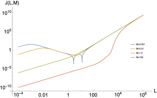
Figure 1: Absolute value of the renormalized current $J=\braket{J}/eaH^{3}$ is shown as a function of $L=eE/H^{2}$. Each line corresponds to different mass parameter $M=m/H$. Negative current is observed in $L=1\sim 10$ for $M=0.001$ case.

3.1 Limiting behaviors

First let us consider various limiting behaviors.

A Weak electric field regime

$eE\ll m^{2},H^{2}$

The renormalized current in this regime is expressed as

$$J\xrightarrow{L\to 0}\frac{L}{12\pi^{2}}\left\{\log M+\frac{8\pi}{3}\frac{\mu_{0}(\mu_{0}^{2}-1)}{\sin(2\pi\mu_{0})}-\frac{1}{2}\left[\psi\left(\frac{1}{2}+\mu_{0}\right)+\psi\left(\frac{1}{2}-\mu_{0}\right)\right]\right\},$$ (3.2)

where $\mu_{0}=\sqrt{9/4-M^{2}}$. The dimensionless conductivity $\sigma(M)=J/L|_{L\to 0}$ is plotted in Fig. 2. The scaling of $\sigma(M)$ is given by

$$\sigma(M)\rightarrow\left\{\begin{array}[]{cc}\dfrac{3}{4\pi^{2}M^{2}}&(M\ll 1)\\ \left(\dfrac{7}{72\pi^{2}M^{2}}+\mathcal{O}(M^{-4})\right)-\mathrm{e}^{-2\pi M}\left(\dfrac{4}{9\pi}M^{3}+\mathcal{O}(M^{1})\right)&(M\gg 1)\end{array}\right..$$ (3.3)

There is a strong $M^{-2}$ enhancement for the small scalar mass. This is a four dimensional analog of the two dimensional IR hyperconductivity reported in [20]. We can also see the $M^{-2}$ scaling for the massive scalar but the coefficient is slightly changed.

The exponentially suppressed term ($\propto\mathrm{e}^{-2\pi M}$) in the large mass regime must exist naturally because the standard Bogoliubov calculation gives the number density of the scalar particles in dS spacetime $n\sim H^{4}(\mathrm{e}^{2\pi M}-1)^{-1}$ which means the exponential suppression of heavy particles. Nevertheless, we also have inexplicable terms which are not protected by exponential factor in the conductivity.

Of course, there is room for changing the renormalization fixing without breaking the condition $\braket{J_{z}}_{\mathrm{ren}}\to 0$ for $M\to\infty$. If one naively tried to remove the $M^{-2}$ term in (3.3), it would cause a huge IR correction and even worse negativity to the renormalized current. Furthermore, if all the unprotected terms should be subtracted from the current $J$, the second term in (3.2) would be left results in a discontinuity at $M=\sqrt{2}$. It is also obvious that $\sigma$ would be negative for $M\gg 1$ in such a treatment. For these reasons, we do not consider changing the renormalization condition.

Note also that this $7/(72\pi^{2}M^{2})$ term corresponds to the fourth order adiabatic term. The terms in (2.20) correspond to the zeroth and second order adiabatic subtraction terms. We can expect that the formal infinite order adiabatic subtraction of the terms proportional to $L$ (WKB is an asymptotic expansion) would result in the removal of the exponentially unprotected behavior in massive limit.

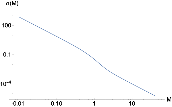
Figure 2: Conductivity of dS spacetime

B Strong electric field or weak curvature regime

$eE\gg m^{2},\,H^{2}$, or $H^{2}\ll m^{2},\,eE$

In this limit, the $L^{3}$ term in the first line of (2.21) and the integration of the digamma functions cancels each other. We find

$$J\simeq\frac{L^{2}}{12\pi^{3}}\mathrm{sgn}(L)\mathrm{e}^{-\frac{\pi M^{2}}{|L|}},$$ (3.4)

and recover the Schwinger’s famous suppression factor $\exp(-\pi m^{2}/eE)$. There is no mass dependence for $L\to\infty$. All the lines in Fig. 1 converge at infinity. Equivalently, this is expressed in terms of dimensionful quantities in Minkowski limit as

$$\braket{J_{z}}_{\mathrm{ren}}\xrightarrow{H\to 0}\frac{e}{12\pi^{2}}(eE)^{2}\frac{1}{H}e^{-\frac{\pi m^{2}}{eE}},$$ (3.5)

where asymptotic analysis reveals that no $\mathcal{O}(H^{0})$ term appears. The divergence $H^{-1}$ is due to the lack of the cosmic dilution in the Minkowski spacetime. The particles produced at $t=-\infty$ contributes to the current expectation value forever, so $H^{-1}$ must be replaced by some regulator such as $(t-t_{0})$ with $t_{0}$ being the turn-on time of the electric field. This prescription is justified because the differentiation $\frac{\mathrm{d}}{\mathrm{d}\eta}\braket{J}$ is finite when $H\to 0$. Note that the conformal time $\eta$ is identical to the cosmic time $t$ in this limit as we are taking the scale factor $a=(1-H\eta)^{-1}$. This behavior corresponds to the result obtained in Minkowski space. This linear growth of the current in time was shown in [28].

3.2 Negativity of the current

Noteworthy is the existence of the negative current $J<0$ around $L\sim\mathcal{O}(1)$ for small mass regime $M\lesssim 10^{-3}$. Typical situation is depicted in Fig. 3. $L=0$ is a trivial zero of $J(L,M)$. Two more zeros of the current appear in $L>0$ and $J$ is negative between them.

The positive current causes negative backreaction to the background electric field as expected. The negative current conversely enhances the background electric field. The current-electric field system can be seen as a sort of feedback system and stability analysis is easy. The first (nontrivial) zero of the current corresponds to the so-called diverging point. No backreaction occurs at this point, however, small deviation from this point induces positive feedback which enhances the deviation. The second zero (and also the trivial zero) is a stable point of the system. Small deviations are pulled back to this point.

Note that negativity of the induced current does not mean fatal instability of the system, as it occurs only in a finite range of the electric field and the induced current recovers its positivity as $L$ increases. The position of the second zero is numerically given by $L=-\frac{1}{3}\log M$ for $M\ll 1$ indeed.

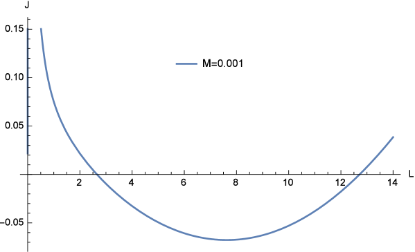
Figure 3: Example of the negativity of the current $J(L,M)$. IR enhancement around $L\sim M$ is not shown here (see the logarithmic plot in Fig. 1). There are three zeros of $J$, two of them ($L=0$ and $L\sim 13$) are stable, the other ($L\sim 2.5$) is unstable.

In Fig. 4, we show the position of the zeros of $J(L,M)$ in $L$-$M$ plane, which also serves as a phase diagram of the current versus electric field. Each line represents the zeros of the current. The lower (upper) line corresponds to the first (second) zero of the current $J(L,M)$. The negativity happens in the region between the two lines. There exists a critical mass $M_{c}\sim 0.0033$, the maximum value of the scalar mass which can cause the negativity of the current. We also emphasize that the negativity is usually mild compared to the IR hyperconductivity which occurs coincidently and the $J\propto L^{2}$ behavior in the strong field regime as we mentioned in previous subsection.

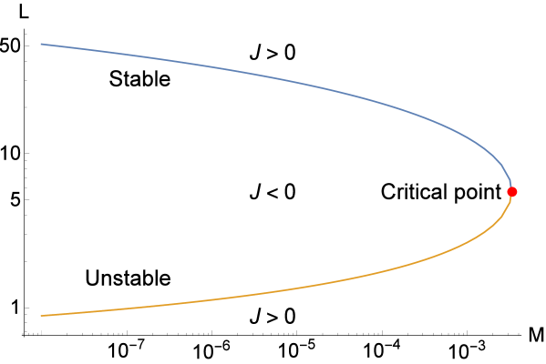
Figure 4: Linear stability analysis of the current-electric field system. The upper (blue) line represents the trajectory of stable points and the lower (orange) line represents that of diverging points. The red dot represents the critical point $(L_{c},M_{c})=(5.7,0.0033)$.

Although we have convinced ourselves that the negative induced current is not dangerous as we intuitively thought, its interpretation is another problem. We must remember that the particle description is correct only in the semiclassical regime, say, $L^{2}+M^{2}\gg 1$. Naively taken, small mass but large electric field regime can satisfy this condition and should be described well by the semiclassical approximation, but it turns out not to be the case. The appearance of the exponentially unprotected terms in weak electric field but massive limit (3.3) is the counterpart of the breakdown of the semiclassical description.

4 Discussion

In this section, we try to clarify the intuitive physical interpretation of the results summarized in the previous section.

We begin with the semiclassical description for the induced current $\braket{J_{z}}$. In the particle picture, $\braket{J_{z}}$ can be split into two parts (see also [20]) as

$$\braket{J_{z}}=J_{\mathrm{pairs}}+J_{\mathrm{vac}},$$ (4.1)

where $J_{\mathrm{pairs}}$ is a contribution due to the kinetic motion of the semiclassical particles and given by $J_{\mathrm{pairs}}=2e\int v\mathrm{d}n$ ($v$ is the velocity and $\mathrm{d}n$ is the differential number density of carriers). $J_{\mathrm{vac}}$ is the vacuum current which flows to satisfy the local current conservation low when the particle pair is produced out of the vacuum. The vacuum current connects the pair particles. In Minkowski spacetime, the positiveness of the semiclassical current is obvious. However, it is not so trivial in de Sitter spacetime due to the dynamics of the charged particles and the spacetime topology. When the charged particles move along the electric field, $J_{\mathrm{pairs}}$ is always positive, but they can move against the electric field (in upstream direction) in de Sitter spacetime. This is due to the effect of the rapid cosmic expansion. Of course, $J_{\mathrm{pairs}}$ itself is expected to be positive because the particle production in the usual (down-stream) direction is more likely than that in the opposite (up-stream) direction even in de Sitter spacetime. Another difference from Minkowski appears in $J_{\mathrm{vac}}$. Since four-dimensional de Sitter spacetime has $\mathbb{R}\times S^{3}$ topology, there is a detour which links two spatially separated points. Thus, the vacuum current can make a detour and contribute negatively, while the vacuum current in a shortcut way is always positive. Since a scalar field with a small mass has a long Compton wavelength, it can detect the global structure of spacetime. If this explanation for the negative current is pertinent, the negativity of the induced current might be found even in a lower dimensional setup such as quantum field theory on a circle.

When it comes to the terms without the exponential mass suppression in (3.3), we cannot make any satisfactory interpretations so far as they are contributions beyond those obtained by the semiclassical approximation or the instanton analysis [29].

5 Conclusion

In the present paper, we have calculated the vacuum expectation value of a charged scalar current in the presence of a constant homogeneous electric field along $z$-direction in de Sitter spacetime using the point-splitting regularization scheme in a covariant and gauge-invariant manner. This enabled us to do renormalization explicitly in the equation of motion. The only divergence we have encountered is the logarithmic divergence which can be absorbed into the kinetic term of the gauge field in a conventional fashion. In a previous calculation done with the momentum cutoff technique [22], there was also a quadratic divergence which was an obstacle to the gauge-invariant renormalization. In [22], the adiabatic subtraction, in which WKB expansion was adopted to imitate the large momentum behavior of the mode function, was applied. Here we have imposed the renormalization condition (2.19) instead of employing the adiabatic subtraction. Interestingly, the result of the minimal subtraction eliminating only the terms in (2.20) and that with the adiabatic subtraction show the perfect agreement. This remarkable fact strongly suggests the correctness of the result.

We have also investigated the properties and the consequences of the renormalized current (2.21). We have found two kinds of the breakdown of the semiclassical approximation. One is the term which is not suppressed by the exponential factor $\mathrm{e}^{-2\pi m/H}$ and it appears in the massive and weak electric field limit, $eE/H^{2}\ll 1,\,m/H\gg 1$. The conventional Bogoliubov calculation indicates that all the terms in this limit should be protected by this exponential factor. The limiting behavior of the (dimensionless) conductivity $\sigma=\braket{J}_{\mathrm{ren}}/(e^{2}aHE)|_{E\to 0}$ in (3.3), however, contains the unprotected terms.

The other is the negativity of the renormalized current which shows up in tiny mass regime $m\lesssim 0.003H$ that has already been discovered by Kobayashi and Afshordi [22] using the adiabatic regularization scheme. It is natural that one might think the negative current of an artifact of the renormalization scheme. Indeed, the adiabatic subtraction scheme breaks down in the IR limit because WKB (adiabatic) approximation is not correct in this regime even though it removes the UV divergences. We have, however, found that the outcome has nothing to do with the accuracy of the WKB approximation, so that we can say that such a criticism does not apply. Therefore, we have to take these strange phenomena seriously.

It should be noted that the expression for the renormalized current (2.21) apparently has a divergence in the massless limit. This is not the problem of our analysis, but merely an outcome of the fact that the vacuum state for an exactly massless charged field in an electromagnetic background is unstable. Of course, there is no divergence in the large mass limit by construction.

We have argued that the uncertainty of the renormalization in curved spacetime comes from the lack of knowledge of the correct behaviors of the quantum fields in some asymptotic region. The only reliable behavior is the asymptotics in Minkowski limit, but it does not fully fix the renormalization condition, although the semiclassical properties are reproduced in this limit, namely, for the cases $L\gg 1$ or $H\ll 1$. Again, this is not the problem of our analysis but rather originates in the lack of information in this curved spacetime. Conversely, the choice of the renormalization condition does not affect the behavior in the flat spacetime.

References

- [1] N. Birrell and P. Davies, Quantum Fields in Curved Space. Cambridge Monographs on Mathematical Physics. Cambridge University Press, 1984.
- [2] V. Mukhanov and S. Winitzki, Introduction to Quantum Effects in Gravity. Cambridge University Press, 2007.
- [3] K. Sato and J. Yokoyama, Inflationary cosmology: First 30+ years, International Journal of Modern Physics D 24 (2015), no. 11 1530025.
- [4] R. Plaga, Detecting intergalactic magnetic fields using time delays in pulses of -rays, 1995.
- [5] K. Ichiki, S. Inoue, and K. Takahashi, Probing the nature of the weakest intergalactic magnetic fields with the high-energy emission of gamma-ray bursts, The Astrophysical Journal 682 (2008), no. 1 127.
- [6] A. Neronov and I. Vovk, Evidence for strong extragalactic magnetic fields from Fermi observations of Tev blazars, Science 328 (2010), no. 5974 73–75.
- [7] I. Vovk, A. M. Taylor, D. Semikoz, and A. Neronov, Fermi/LAT Observations of 1ES 0229+200: Implications for Extragalactic Magnetic Fields and Background Light, The Astrophysical Journal Letters 747 (2012), no. 1 L14.
- [8] K. Takahashi, M. Mori, K. Ichiki, and S. Inoue, Lower Bounds on Intergalactic Magnetic Fields from Simultaneously Observed GeV-TeV Light Curves of the Blazar Mrk 501, The Astrophysical Journal Letters 744 (2012), no. 1 L7.
- [9] H. Tashiro, W. Chen, F. Ferrer, and T. Vachaspati, Search for CP violating signature of intergalactic magnetic helicity in the gamma-ray sky, Monthly Notices of the Royal Astronomical Society: Letters 445 (2014), no. 1 L41–L45.
- [10] T. Akahori, K. Kumazaki, K. Takahashi, and D. Ryu, Exploring the intergalactic magnetic field by means of faraday tomography, Publications of the Astronomical Society of Japan 66 (2014), no. 3 [http://pasj.oxfordjournals.org/content/66/3/65.full.pdf+html].
- [11] D. H. F. M. Schnitzeler, The latitude dependence of the rotation measures of nvss sources, Monthly Notices of the Royal Astronomical Society: Letters 409 (2010), no. 1 L99–L103, [http://mnrasl.oxfordjournals.org/content/409/1/L99.full.pdf+html].
- [12] B. Ratra, Cosmological ’seed’ magnetic field from inflation, The Astrophysical Journal 391 (1992) L1–L4.
- [13] M. Turner and L. Widrow, Inflation-produced, large-scale magnetic fields, Phys. Rev. D 37 (May, 1988) 2743–2754.
- [14] K. Bamba and J. Yokoyama, Large-scale magnetic fields from inflation in dilaton electromagnetism, Phys. Rev. D 69 (Feb, 2004) 043507.
- [15] K. Bamba and J. Yokoyama, Large-scale magnetic fields from dilaton inflation in noncommutative spacetime, Phys. Rev. D 70 (Oct, 2004) 083508.
- [16] J. Martin and J. Yokoyama, Generation of large scale magnetic fields in single-field inflation, Journal of Cosmology and Astroparticle Physics 2008 (2008), no. 01 025.
- [17] V. Demozzi, V. Mukhanov, and H. Rubinstein, Magnetic fields from inflation?, Journal of Cosmology and Astroparticle Physics 2009 (2009), no. 08 025.
- [18] J. Schwinger, On gauge invariance and vacuum polarization, Physical Review 82 (1951), no. 5 664.
- [19] J. Garriga, Pair production by an electric field in (1+1)-dimensional de Sitter space, Phys. Rev. D 49 (Jun, 1994) 6343–6346.
- [20] M. B. Fröb, J. Garriga, S. Kanno, M. Sasaki, J. Soda, T. Tanaka, and A. Vilenkin, Schwinger effect in de Sitter space, Journal of Cosmology and Astroparticle Physics 2014 (2014), no. 04 009.
- [21] R.-G. Cai and S. P. Kim, One-Loop Effective Action and Schwinger Effect in (Anti-) de Sitter Space, JHEP 09 (2014) 072, [arXiv:1407.4569].
- [22] T. Kobayashi and N. Afshordi, Schwinger effect in 4D de Sitter space and constraints on magnetogenesis in the early universe, Journal of High Energy Physics 2014 (2014), no. 10 1–36.
- [23] C. Stahl, E. Strobel, and S.-S. Xue, Fermionic current and Schwinger effect in de Sitter spacetime, arXiv:1507.0168.
- [24] E. Bavarsad, C. Stahl, and S.-S. Xue, Scalar current of created pairs by Schwinger mechanism in de Sitter spacetime, arXiv:1602.0655.
- [25] T. Hayashinaka, T. Fujita, and J. Yokoyama, Fermionic Schwinger effect and induced current in de Sitter space, arXiv:1603.0416.
- [26] B. S. DeWitt, Quantum field theory in curved spacetime, Physics Reports 19 (1975), no. 6 295–357.
- [27] I. S. Gradshteyn and I. M. Ryzhik, Table of integrals, series, and products. Elsevier/Academic Press, Amsterdam, seventh ed., 2007.
- [28] P. R. Anderson and E. Mottola, Instability of global de Sitter space to particle creation, Phys. Rev. D89 (2014) 104038, [arXiv:1310.0030].
- [29] A. R. Brown, Schwinger pair production at nonzero temperatures or in compact directions, arXiv:1512.0571.