Collision Avoidance for Bi-Steerable Car Using Analytic Left Inversion

Abstract

A case study is presented of a collision avoidance system that directly integrates the kinematics of a bi-steerable car with a suitable path planning algorithm. The first step is to identify a path using the method of rapidly exploring random trees, and then a spline approximation is computed. The second step is to solve the output tracking problem by explicitly computing the left inverse of the kinematics of the system to render the Taylor series of the desired input for each polynomial section of the spline approximation. The method is demonstrated by numerical simulation.

I Introduction

A convergence of technological advances in conjunction with changing societal attitudes suggests that autonomous wheeled vehicles are poised to soon enter main stream applications in business, the government, and the private realm [10]. As this happens, it is likely that vehicle design will evolved in new directions once the human driver and passengers are completely replaced by a computer control system and cargo. For example, a bi-steerable car with independent front and rear axels provides improved maneuverability and handling, which would be invaluable in urban settings to improve collision avoidance [11, 12, 19, 21, 22, 20, 25]. But such improved performance is predicated on control methodologies that properly combine the true dynamics of the vehicle with the proper path planning tools [1, 16].

In this paper, a case study is presented of a collision avoidance system that directly integrates the kinematics of a bi-steerable car with a suitable path planning algorithm. Here collision avoidance means simply steering a vehicle modeled as a point from a starting location to a final location while avoiding all stationary obstacles in between the two locations. The first step is solving the path planning problem. Numerous algorithms appear in the literature which are applicable to the collision avoidance problem, such as rapidly exploring random trees (RRT), probabilistic roadmap (PRM), artificial potential fields, and genetic algorithms [16]. The second step is solving the output tracking problem. That is, determine the control inputs so that the vehicle accurately follows the desired path. Mathematically, this corresponds to computing a left inverse for the system. There is an extensive literature on this topic in the context of geometric nonlinear control theory, see, for example, [3, 5, 13, 14, 15, 23, 24]. This class of techniques generates left inverses dynamically by driving a certain inverse dynamical system with the desired output. While very convenient in some situations, this method has certain limitations, like requiring the system to be minimum phase. In addition, this approach does not provide an explicit representation of the control input one is seeking. Another common approach is to use the property of flatness, which allows one to explicitly compute a left inverse analytically provided suitable flat outputs can be identified [4, 17]. Unfortunately, these output are sometimes not the most desirable from a physical point of view. This turns out to the case for the bi-steerable car, where the flat outputs do not correspond to simple physical variables like a center point on the vehicle or its speed or orientation [12, 21, 22, 20]. This then makes integrating the tracking problem with path planning problem more complex. A final inversion method, which is the one employed in this paper, is to use an analytic expression for the left inverse which is available for systems which have a well defined vector relative degree for the outputs of interest [8, 7]. They do not have to be flat outputs. The method is based on a Fliess operator representation of input-output system, and a combinatorial Hopf algebra technique that renders an explicit formula for the Taylor series of the left inverse when the output is an analytic function in the range of the input-output map. This single formula can be pre-computed efficiently off-line to arbitrary precision [2, 6], and, for example, could be hardwired on an FPGA for real-time implementation. In this setting, the desired output trajectory is approximated by a spline, and then the left inverse of each polynomial section is numerically evaluated using the inversion formula. It will be shown here that this strategy provides a feasible and accurate solution to the collision avoidance problem for a bi-steerable car. For brevity, only the vehicle’s kinematics are considered.

The paper is organized as follows. In Section II, preliminaries concerning Fliess operators and their inverses are briefly summarized to make the presentation more self-contained. Then, in Section III, the left inverse of the kinematics of the bi-steerable car is computed. This result is then integrated in Section IV with the RRT path planning algorithm and the corresponding numerical simulations are presented. Section V provides the paper’s conclusions.

II Preliminaries

In this section, some preliminaries concerning the theory of Fliess operators are outlined as they provide the cornerstone for the method presented in this paper. The interested reader is referred to [9, 8] for a more complete treatment.

II-A Fliess Operators and Their Interconnections

A finite nonempty set of noncommuting symbols $X=\{x_{0},x_{1},$ $\ldots,x_{m}\}$ is called an alphabet. Each element of $X$ is called a letter, and any finite sequence of letters from $X$, $\eta=x_{i_{1}}\cdots x_{i_{k}}$, is called a word over $X$. The length of $\eta$, $\left|\eta\right|$, is the number of letters in $\eta$. The set of all words with length $k$ is denoted by $X^{k}$. The set of all words including the empty word, $\emptyset$, is designated by $X^{\ast}$. It forms a monoid under catenation. The set $\eta X^{\ast}$ is comprised of all words with the prefix $\eta$. Any mapping $c:X^{\ast}\rightarrow{\mathbb{R}}^{\ell}$ is called a formal power series. The value of $c$ at $\eta\in X^{\ast}$ is written as $(c,\eta)$ and called the coefficient of $\eta$ in $c$. Typically, $c$ is represented as the formal sum $c=\sum_{\eta\in X^{\ast}}(c,\eta)\eta.$ If the constant term $(c,\emptyset)=0$ then $c$ is said to be proper. The support of $c$, ${\rm supp}(c)$, is the set of all words having nonzero coefficients. The collection of all formal power series over $X$ is denoted by ${\mathbb{R}}^{\ell}\langle\langle X\rangle\rangle$. It forms an associative ${\mathbb{R}}$-algebra under the catenation product and a commutative and associative ${\mathbb{R}}$-algebra under the shuffle product, denoted here by ${\scriptscriptstyle\;\sqcup\sqcup\;}$. The latter is the ${\mathbb{R}}$-bilinear extension of the shuffle product of two words, which is defined inductively by $(x_{i}\eta){\scriptscriptstyle\;\sqcup\sqcup\;}(x_{j}\xi)=x_{i}(\eta{\scriptscriptstyle\;\sqcup\sqcup\;}(x_{j}\xi))+x_{j}((x_{i}\eta){\scriptscriptstyle\;\sqcup\sqcup\;}\xi)$ with $\eta{\scriptscriptstyle\;\sqcup\sqcup\;}\emptyset=\emptyset{\scriptscriptstyle\;\sqcup\sqcup\;}\eta=\eta$ for all $\eta,\xi\in X^{\ast}$ and $x_{i},x_{j}\in X$.

One can formally associate with any series $c\in\mbox{${\mathbb{R}}^{\ell}\langle\langle X\rangle\rangle$}$ a causal $m$-input, $\ell$-output operator, $F_{c}$, in the following manner. Let $\mathfrak{p}\geq 1$ and $t_{0}<t_{1}$ be given. For a Lebesgue measurable function $u:[t_{0},t_{1}]\rightarrow{\mathbb{R}}^{m}$, define $\|u\|_{\mathfrak{p}}=\max\{\|u_{i}\|_{\mathfrak{p}}:\ 1\leq i\leq m\}$, where $\|u_{i}\|_{\mathfrak{p}}$ is the usual $L_{\mathfrak{p}}$-norm for a measurable real-valued function, $u_{i}$, defined on $[t_{0},t_{1}]$. Let $L^{m}_{\mathfrak{p}}[t_{0},t_{1}]$ denote the set of all measurable functions defined on $[t_{0},t_{1}]$ having a finite $\|\cdot\|_{\mathfrak{p}}$ norm and $B_{\mathfrak{p}}^{m}(R)[t_{0},t_{1}]:=\{u\in L_{\mathfrak{p}}^{m}[t_{0},t_{1}]:\|u\|_{\mathfrak{p}}\leq R\}$. Assume $C[t_{0},t_{1}]$ is the subset of continuous functions in $L_{1}^{m}[t_{0},t_{1}]$. Define inductively for each $\eta\in X^{\ast}$ the map $E_{\eta}:L_{1}^{m}[t_{0},t_{1}]\rightarrow C[t_{0},t_{1}]$ by setting $E_{\emptyset}[u]=1$ and letting

$$E_{x_{i}\bar{\eta}}[u](t,t_{0})=\int_{t_{0}}^{t}u_{i}(\tau)E_{\bar{\eta}}[u](\tau,t_{0})\,d\tau,$$

where $x_{i}\in X$, $\bar{\eta}\in X^{\ast}$, and $u_{0}=1$. The input-output system corresponding to $c$ is the Fliess operator

$$F_{c}[u](t)=\sum_{\eta\in X^{\ast}}(c,\eta)\,E_{\eta}[u](t,t_{0}).$$

If there exist real numbers $K_{c},M_{c}>0$ such that $\left|(c,\eta)\right|\leq K_{c}M_{c}^{|\eta|}|\eta|!$, $\forall\eta\in X^{\ast}$, then $F_{c}$ constitutes a well defined mapping from $B_{\mathfrak{p}}^{m}(R)[t_{0},$ $t_{0}+T]$ into $B_{\mathfrak{q}}^{\ell}(S)[t_{0},\,t_{0}+T]$ for sufficiently small $R,T>0$, where the numbers $\mathfrak{p},\mathfrak{q}\in[1,\infty]$ are conjugate exponents, i.e., $1/\mathfrak{p}+1/\mathfrak{q}=1$. (Here, $\left|z\right|:=\max_{i}\left|z_{i}\right|$ when $z\in{\mathbb{R}}^{\ell}$.) The set of all such locally convergent series is denoted by ${\mathbb{R}}^{\ell}_{LC}\langle\langle X\rangle\rangle$. On the other hand, if $\left|(c,\eta)\right|\leq K_{c}M_{c}^{|\eta|}$, $\forall\eta\in X^{\ast}$, then the operator is well defined over $[0,T]$ for all $R,T>0$. These are called globally convergent series, and the set of all such series is denoted by ${\mathbb{R}}^{\ell}_{GC}\langle\langle X\rangle\rangle$. A Fliess operator $F_{c}$ defined on $B_{\mathfrak{p}}^{m}(R)[t_{0},t_{0}+T]$ is said to be realized by a state space realization

$$\dot{z} =g_{0}(z)+\sum_{i=1}^{m}g_{i}(z)\,u_{i},\;\;z(t_{0})=z_{0}$$ (1a)

$$y =h(z),$$ (1b)

where each $g_{i}$ is an analytic vector field expressed in local coordinates on some neighborhood ${\cal W}\subseteq{\mathbb{R}}^{n}$ of $z_{0}$, and $h$ is an analytic function on ${\cal W}$, if (1a) has a well defined solution $z(t)$, $t\in[t_{0},t_{0}+T]$ on ${\cal W}$ for any given input $u\in B_{\mathfrak{p}}^{m}(R)[t_{0},t_{0}+T]$, and

$$F_{c}[u](t)=h(z(t)),\;\;t\in[t_{0},t_{0}+T].$$

In this case, the coefficients of the $i$-th component of generating series $c$ are computed by

$$(c_{i},\eta)=L_{g_{\eta}}h_{i}(z_{0}),\;\;\eta\in X^{\ast},$$ (2)

where

$$L_{g_{\eta}}h_{i}:=L_{g_{j_{1}}}\cdots L_{g_{j_{k}}}h_{i},\;\;\eta=x_{j_{k}}\cdots x_{j_{1}},$$

the Lie derivative of $h_{i}$ with respect to $g_{j}$ is defined as

$$L_{g_{j}}h_{i}:W\rightarrow{\mathbb{R}}:z\mapsto\frac{\partial h_{i}}{\partial z}(z)\,g_{j}(z),$$

and $L_{g_{\emptyset}}h_{i}=h_{i}$.

When Fliess operators $F_{c}$ and $F_{d}$ are connected in a parallel-product fashion, it is known that $F_{c}F_{d}=F_{c{\scriptscriptstyle\;\sqcup\sqcup\;}d}$. If $F_{c}$ and $F_{d}$ with $c\in\mbox{${\mathbb{R}}^{\ell}\langle\langle X\rangle\rangle$}$ and $d\in\mbox{${\mathbb{R}}^{m}\langle\langle X\rangle\rangle$}$ are interconnected in a cascade manner, the composite system $F_{c}\circ F_{d}$ has the Fliess operator representation $F_{c\circ d}$, where $c\circ d$ denotes the composition product of $c$ and $d$ as described in [8]. This product is associative and ${\mathbb{R}}$-linear in its left argument $c$. In the event that two Fliess operators are interconnected to form a feedback system, the closed-loop system has a Fliess operator representation whose generating series is the feedback product of $c$ and $d$, denoted by $c@d$. This product can be explicitly computed via Hopf algebra methods. The basic idea is to consider the set of operators $\mathscr{F}_{\delta}=\{I+F_{c}\;:\;c\in\mbox{${\mathbb{R}}^{m}\langle\langle X\rangle\rangle$}\}$, where $I$ denotes the identity map, as a group under composition. It is convenient to introduce the symbol $\delta$ as the (fictitious) generating series for the identity map. That is, $F_{\delta}:=I$ such that $I+F_{c}:=F_{\delta+c}=F_{c_{\delta}}$ with $c_{\delta}:=\delta+c$. The set of all such generating series for $\mathscr{F}_{\delta}$ is denoted by ${\mathbb{R}}\langle\langle X_{\delta}\rangle\rangle$. This set also forms a group under the composition product induced by operator composition, namely, $c_{\delta}\circ d_{\delta}:=\delta+d+c\>\tilde{\circ}\,d$, where $\>\tilde{\circ}\,$ denotes the modified composition product [8]. The group $(\mbox{${\mathbb{R}}\langle\langle X_{\delta}\rangle\rangle$},\circ,\delta)$ has coordinate functions that form a Faà di Bruno type Hopf algebra. In which case, the group (composition) inverse $c_{\delta}^{\circ-1}$ can be computed efficiently via the antipode of this Hopf algebra [2, 6, 8]. This inverse also provide an explicit expression for the feedback product, namely, $c@d=c\circ(\delta-d\circ c)^{\circ-1}$.

II-B Left Inversion of Multivariable Fliess Operators

It was shown in [26] that $F_{c}$ will map every input which is analytic at $t_{0}$ to an output which is also analytic at $t_{0}$ provided $c\in\mbox{${\mathbb{R}}^{\ell}_{LC}\langle\langle X\rangle\rangle$}$. In [7] an explicit formula was developed for calculating the left inverse of a multivariable mapping $F_{c}$ given a real analytic function in its range. Without loss of generality assume $t_{0}=0$. Note that every $c\in\mbox{${\mathbb{R}}\langle\langle X\rangle\rangle$}$ can be decomposed into its natural and forced components, that is, $c=c_{N}+c_{F}$, where $c_{N}:=\sum_{k\geq 0}(c,x_{0}^{k})x_{0}^{k}$ and $c_{F}:=c-c_{N}$. A condition under which the left inverse of $F_{c}$ exists is provided by the following definition

Definition 1

Given $c\in\mbox{${\mathbb{R}}^{m}\langle\langle X\rangle\rangle$}$, let $r_{i}\geq 1$ be the largest integer such that ${\rm supp}(c_{F,i})\subseteq x_{0}^{r_{i}-1}X^{\ast}$, where $i=1,2,\ldots,m$. Then the component series $c_{i}$ has relative degree $r_{i}$ if the linear word $x_{0}^{r_{i}-1}x_{j}\in{\rm supp}(c_{i})$ for some $j\in\{1,\ldots,m\}$, otherwise it is not well defined. In addition, $c$ has vector relative degree $r=[r_{1}\;r_{2}\;\cdots\;r_{m}]$ if each $c_{i}$ has relative degree $r_{i}$ and the $m\times m$ matrix

$$\footnotesize A=\left[\begin{tabular}[]{@{ }c@{$\;\;$ }c@{$\;\;$}c@{$\;\;$}c@{ }}$(c_{1},x_{0}^{r_{1}-1}x_{1})$&$(c_{1},x_{0}^{r_{1}-1}x_{2})$&$\cdots$&$(c_{1},x_{0}^{r_{1}-1}x_{m})$\\ $(c_{2},x_{0}^{r_{2}-1}x_{1})$&$(c_{2},x_{0}^{r_{2}-1}x_{2})$&$\cdots$&$(c_{2},x_{0}^{r_{2}-1}x_{m})$\\ $\vdots$&$\vdots$&$\vdots$&$\vdots$\\ $(c_{m},x_{0}^{r_{m}-1}x_{1})$&$(c_{m},x_{0}^{r_{m}-1}x_{2})$&$\cdots$&$(c_{m},x_{0}^{r_{m}-1}x_{m})$\end{tabular}\right]$$

has full rank. Otherwise, $c$ does not have vector relative degree.

This notion of vector relative degree agrees with the usual definition in the state space setting [15]. In particular, $c$ has vector relative degree $r$ only if for each $i$ the series $(x_{0}^{r_{i}-1}x_{j})^{-1}(c_{i})$ is non proper for some $j$. Here the left-shift operator for any $x_{i}\in X$ is defined on $X^{\ast}$ by $x_{i}^{-1}(x_{i}\eta)=\eta$ with $\eta\in X^{\ast}$ and zero otherwise. Higher order shifts are defined inductively via $(x_{i}\xi)^{-1}(\cdot)=\xi^{-1}x_{i}^{-1}(\cdot)$, where $\xi\in X^{\ast}$. The left-shift operator is assumed to act linearly and componentwise on ${\mathbb{R}}^{m}\langle\langle X\rangle\rangle$. The shuffle inverse of any series $C\in\mbox{${\mathbb{R}}^{m\times m}\langle\langle X\rangle\rangle$}$ is given by

$$C^{{\scriptscriptstyle\;\sqcup\sqcup\;}-1}=((C,\emptyset)(I-C^{\prime}))^{{\scriptscriptstyle\;\sqcup\sqcup\;}-1}=(C^{\prime})^{{\scriptscriptstyle\;\sqcup\sqcup\;}\ast}(C,\emptyset)^{-1},$$

where $C^{\prime}=I-(C,\emptyset)^{-1}C$ is proper, i.e., $(C^{\prime},\emptyset)=0$, and $(C^{\prime})^{{\scriptscriptstyle\;\sqcup\sqcup\;}\ast}:=\sum_{k\geq 0}(C^{\prime})^{{\scriptscriptstyle\;\sqcup\sqcup\;}k}$. The relationship between $C^{{\scriptscriptstyle\;\sqcup\sqcup\;}-1}$ and the multiplicative inverse operator $(F_{C})^{-1}$, that is, $F_{C}(F_{C})^{-1}=(F_{C})^{-1}F_{C}=I$, is $(F_{C})^{-1}=F_{C^{{\scriptscriptstyle\;\sqcup\sqcup\;}-1}}$.

Let $X_{0}:=\{x_{0}\}$, and ${\mathbb{R}}[[X_{0}]]$ denotes the set of all commutative series over $X_{0}$. When $c\in\mbox{${\mathbb{R}}[[X_{0}]]$}$, $F_{c}[u](t)$ reduces to the Taylor series $\sum_{k\geq 0}(c,x_{0}^{k})E_{x_{0}^{k}}[u](t)=\sum_{k\geq 0}(c,x_{0}^{k})t^{k}/k!$. The main inversion tool used in the paper is given next.

Theorem 1

Suppose $c\in\mbox{${\mathbb{R}}^{m}\langle\langle X\rangle\rangle$}$ has vector relative degree $r$. Let $y$ be analytic at $t=0$ with generating series $c_{y}\in\mbox{${\mathbb{R}}^{m}_{LC}[[X_{0}]]$}$ satisfying $(c_{y_{i}},x_{0}^{k})=(c_{i},x_{0}^{k})$, $k=0,1,\ldots,r_{i}-1$, $i=1,2,\ldots,m$. Then the input

$$u(t)=\sum_{k=0}^{\infty}(c_{u},x_{0}^{k})\frac{t^{k}}{k!},$$ (3)

is the unique real analytic solution to $F_{c}[u]=y$ on $[0,T]$ for some $T>0$, where

$$c_{u}=\left(\left[C^{{\scriptscriptstyle\;\sqcup\sqcup\;}-1}{\scriptscriptstyle\;\sqcup\sqcup\;}(x_{0}^{r})^{-1}(c-c_{y})\right]^{\circ-1}\right)_{N},$$ (4)

the $i$-th row of $(x_{0}^{r})^{-1}(c-c_{y})$ is $(x_{0}^{r_{i}})^{-1}(c_{i}-c_{y_{i}})$, and the $(i,j)$-th entry of $C$ is $(x_{0}^{r_{i}-1}x_{j})^{-1}(c_{i})$.

Observe that this theorem describes the outputs that can be successfully tracked by $F_{c}$, namely, those whose Taylor series coefficients satisfy certain matching conditions. (The same conditions appear in the classical papers on dynamic inversion.) For example, if $m=2$ and the vector relative degree is $(2,2)$, the Taylor series of the output are subject to the constraints $(c_{y_{1}},\emptyset)=(c_{1},\emptyset)$, $(c_{y_{2}},\emptyset)=(c_{2},\emptyset)$, $(c_{y_{1}},x_{0})=(c_{1},x_{0})$, and $(c_{y_{2}},x_{0})=(c_{2},x_{0})$, which in turn puts constraints on the class of admissible output paths.

III Left Inverse of Bi-steerable Car Kinematics

Consider the bi-steerable car shown in Figure 1. For simplicity, only the kinematics are considered. So the car is assumed to have zero mass and move in the plane with the speed of the car $u_{1}=\sqrt{\dot{x}^{2}+\dot{y}^{2}}$ and the front axle steering angular velocity $u_{2}=\alpha$ as inputs.

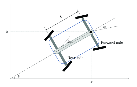
Figure 1: Bi-steerable car

The kinematics of the system are therefore

$$\dot{x} =u_{1}\cos(\theta+\alpha),$$

$$\dot{y} =u_{1}\sin(\theta+\alpha),$$

$$\dot{\theta} =u_{1}\frac{\sin(\alpha-f(\alpha))}{L\cos(f(\alpha))},$$

$$\dot{\alpha} =u_{2},$$

where $f(\alpha):=k\alpha$ with $k\in{\mathbb{R}}$. These dynamics assume the usual constraints of rolling without slippage of the wheels, namely,

$$0= \dot{y}_{forward}\cos(\theta+\alpha)-\dot{x}_{forward}\sin(\theta+\alpha),$$

$$0= \dot{y}_{rear}\cos(\theta+f(\alpha))-\dot{x}_{rear}\sin(\theta+f(\alpha)).$$

Setting $z_{1}=x$, $z_{2}=y$, $z_{3}=\theta$, $z_{4}=\alpha$, the outputs are picked to be the coordinates of the front axle center $y_{i}=z_{i}$, $i=1,2$. The corresponding two-input, two-output state space realization is

$$\left(\begin{array}[]{c}\dot{z_{1}}\\ \dot{z_{2}}\\ \dot{z_{3}}\\ \dot{z_{4}}\end{array}\right) =\left(\begin{array}[]{c}\cos(z_{3}+z_{4})\\ \sin(z_{4}+z_{4})\\ \frac{\sin((1-k)\alpha)}{L\cos(k\alpha)}\\ 0\end{array}\right)u_{1}+\left(\begin{array}[]{c}0\\ 0\\ 0\\ 1\end{array}\right)u_{2}$$ (5m)

$$\left(\begin{array}[]{c}y_{1}\\ y_{2}\end{array}\right) =\left(\begin{array}[]{c}z_{1}\\ z_{2}\end{array}\right).$$ (5r)

Hereafter, the focus is on the $k=-0.7$ case, which as explained in [20] is sufficient for the existence of flat outputs. But this fact in inconsequential here since flat outputs will not be used. The generating series, $c$, can be computed directly from (2) using the vector fields and output function given in (5):

$$c_{1}=z_{1,0}+{\rm co}\,x_{1}-\frac{\sin(1.7z_{4,0})}{\cos(0.7z_{4,0})}\,{\rm si}\,x_{1}^{2}-{\rm si}\,x_{1}x_{2}$$

$$-{{\rm co}}\,x_{1}x_{2}x_{2}-\frac{\sin(1.7z_{4,0})}{\cos(0.7z_{4,0})}\,{\rm co}\,x_{1}x_{2}x_{1}+\cdots$$

$$c_{2}=z_{2,0}+{\rm si}\,x_{1}+\frac{\sin(1.7z_{4,0})}{\cos(0.7z_{4,0})}\,{\rm co}\,x_{1}^{2}+{\rm co}\,x_{1}x_{2}$$

$$-{{\rm si}}\,x_{1}x_{2}x_{2}-\frac{\sin(1.7z_{4,0})}{\cos(0.7z_{4,0})}\,{\rm si}\,x_{1}x_{2}x_{1}+\cdots,$$

where ${\rm co}:=\cos(z_{3,0}+z_{4,0})$ and ${\rm si}:=\sin(z_{3,0}+z_{4,0})$.

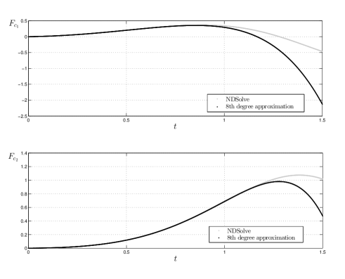
Figure 2: Mathematica computed (NDSolve) and Fliess operator approximated (degree 8) step response of bi-steerable car ($u_{1}(t)=1.5$ and $u_{2}(t)=0.8$, $t>0$)

In this case, $c\in{\mathbb{R}}_{GC}^{2}\langle\langle X\rangle\rangle$ with $X=\{x_{0},x_{1},x_{2}\}$ since all sines and cosines in the numerator of every coefficient can be bounded by $1$. Therefore, after some additional calculations a conservative choice for the growth constants is $K_{c}=\max\{z_{1,0},z_{2,0}\}$ and $M_{c}=2.4\sec(0.7z_{4,0})$. With $z_{1,0}=z_{2,0}=z_{3,0}=0$, $z_{4,0}=z_{5,0}=0.2$, the step response ($u_{1}(t)=1.5$ and $u_{2}(t)=0.8$, $t>0$) of the system was computed using the NDSolve Mathematica function [18] and is compared against a degree eight Fliess operator approximation in Figure 2. Since $c\in{\mathbb{R}}_{GC}^{2}\langle\langle X\rangle\rangle$, the output $y=F_{c}[u]$ is well defined on $[0,\infty)$ for all $u\in B_{1}^{m}[0,T](R)$ and any finite $R,T>0$. [27].

A simple calculation shows that the relative degrees of $y_{1}$ and $y_{2}$ are both one, but the system does not have a well defined vector relative degree. Applying dynamic extension on $u_{1}$ yields the augmented system

$$\left(\begin{array}[]{c}\dot{z_{1}}\\ \dot{z_{2}}\\ \dot{z_{3}}\\ \dot{z_{4}}\\ \dot{z_{5}}\end{array}\right)\!=\!\left(\begin{array}[]{c}z_{5}\cos(z_{3}+z_{4})\\ z_{5}\sin(z_{4}+z_{4})\\ z_{5}\frac{\sin((1-k)\alpha)}{L\cos(k\alpha)}\\ 0\\ 0\end{array}\right)\!+\!\left(\begin{array}[]{c}0\\ 0\\ 0\\ 1\\ 0\end{array}\right)u_{2}\!+\!\left(\begin{array}[]{c}0\\ 0\\ 0\\ 0\\ 1\end{array}\right)\bar{u}_{1},$$ (26)

where the new input $\bar{u}_{1}$ is taken as the derivative of the original input $u_{1}$. This system has vector relative degree $r=[r_{1}\;r_{2}]=[2\;2]$ with $r_{1}+r_{2}=4<5=n$ and generating series

$$c_{1}= \,z_{1,0}+z_{5,0}\,{\rm co}\,x_{0}+z_{5,0}\,{\rm si}\,x_{0}x_{1}+{\rm co}\,x_{0}x_{2}$$

$$-z_{5,0}^{2}\frac{\sin(1.7z_{4,0})}{\cos(0.7z_{4,0})}\,{\rm si}\,x_{0}^{2}+\cdots$$

$$c_{2}= \,z_{2,0}+z_{5,0}\,{\rm si}\,x_{0}+z_{5,0}\,{\rm co}\,x_{0}x_{1}+{\rm si}\,x_{0}x_{2}$$

$$+z_{5,0}^{2}\frac{\sin(1.7z_{4,0})}{\cos(0.7z_{4,0})}\,{\rm co}\,x_{0}^{2}+\cdots.$$

These series are also elements of ${\mathbb{R}}_{GC}^{2}\langle\langle X\rangle\rangle$ since again all sines and cosines in the numerator can be bounded by $1$ so that conservative growth constants are $K_{c}=\max\{z_{1,0},z_{2,0},z_{5,0}\}$ and $M_{c}=2.4z_{5,0}\sec(0.7z_{4,0})$. The decoupling matrix

$$A=(C,\emptyset)=\left(\begin{array}[]{cc}z_{5,0}\,{\rm si}&{\rm co}\\ z_{5,0}\,{\rm co}&{\rm si}\end{array}\right)$$ (27)

is clearly nonsingular as long as $z_{5,0}\neq 0$.

Given a desired output function

$$y(t) =\sum_{k=0}^{\infty}(c_{y},x_{0}^{k})\frac{t^{k}}{k!},$$ (28)

where $c_{y}=[c_{y_{1}},c_{y_{2}}]^{T}$ is the generating series of $y$, the left inverse $c_{u}=[c_{\bar{u}_{1}},c_{u_{2}}]^{T}$ is computed directly from (3)-(4). It is sufficient here to consider polynomial outputs up to degree three, so let $(c_{y_{j}},x_{0}^{i})=v_{ij}$ for $i=0,1,2,3$ and $j=1,2$. The series

$$d=\left(\begin{array}[]{c}d_{1}\\ d_{2}\end{array}\right):=C^{{\scriptscriptstyle\;\sqcup\sqcup\;}-1}{\scriptscriptstyle\;\sqcup\sqcup\;}(x_{0}^{r})^{-1}(c-c_{y})$$

is found to be

$$d_{1}=\frac{v_{12}\,{\rm si}}{z_{5,0}}-\frac{v_{22}\,{\rm co}}{z_{5,0}}+z_{5,0}\frac{\sin(1.7z_{4,0})}{\cos(0.7z_{4,0})}$$

$$+\left(\left(\frac{v_{13}}{z_{5,0}}+v_{22}\frac{\sin(1.7z_{4,0})}{\cos(0.7z_{4,0})}\right)\,{\rm si}\right.$$

$$\left.+\left(v_{12}\frac{\sin(1.7z_{4,0})}{\cos(0.7z_{4,0})}-\frac{v_{23}}{z_{5,0}}\right)\,{\rm co}\right)x_{0}$$

$$+\left(\frac{v_{22}\,{\rm si}}{z_{5,0}}+1.7z_{5,0}\frac{\cos(1.7z_{4,0})}{\cos(0.7z_{4,0})}\right.$$

$$\left.+0.7z_{5,0}\frac{\sin(1.7z_{4,0})\tan(0.7z_{4,0})}{\cos(0.7z_{4,0})}+\frac{v_{22}\,{\rm co}}{z_{5,0}}\right)x_{1}$$

$$+\left(\frac{v_{22}\,{\rm co}}{z_{5,0}^{2}}-\frac{v_{12}\,{\rm co}}{z_{5,0}^{2}}+\frac{\sin(1.7z_{4,0})}{\cos(0.7z_{4,0})}\right)x_{2}+\cdots,$$

$$d_{2}=-v_{12}\,{\rm co}-v_{22}\,{\rm si}$$

$$-\left(v_{13}{\rm co}-z_{5,0}\frac{\sin(1.7z_{4,0})}{\cos(0.7z_{4,0})}\left(v_{22}\,{\rm co}+v_{12}\,{\rm si}\right)+v_{23}{\rm si}\right)x_{0}$$

$$+\left(v_{12}\,{\rm si}-v_{22}\,{\rm co}\right)x_{1}+\cdots$$

The composition inverse of $d$ is computed componentwise using the recursive method in [2, 6, 8]. In which case, the formulas for $c_{\bar{u}_{1}}$ and $c_{u_{2}}$ are, respectively,

$$c_{\bar{u}_{1}}=\left(d_{1}^{\circ{-1}}\right)_{N}=\frac{v_{22}{\rm si}}{z_{5,0}}-\frac{v_{12}{\rm co}}{z_{5,0}}-z_{5,0}\frac{\sin(1.7z_{4,0})}{\cos(0.7z_{4,0})}$$

$$+\frac{1}{z_{5,0}^{2}}\left(\rule{0.0pt}{14.45377pt}-2v_{12}v_{22}\cos(2(z_{3,0}+z_{4,0}))\right.$$

$$+1.7z_{5,0}^{4}\frac{\sin(1.7z_{4,0})\cos(1.7z_{4,0})}{\cos(0.7z_{4,0})^{2}}-v_{13}z_{5,0}\,{\rm si}$$

$$+1.7v_{12}z_{5,0}^{2}\frac{\cos(1.7z_{4,0})}{\cos(0.7z_{4,0})}\,{\rm si}-v_{22}z_{5,0}^{2}\frac{\sin(1.7z_{4,0})}{\cos(0.7z_{4,0})}\,{\rm si}$$

$$+v_{12}^{2}\sin(2(z_{3,0}+z_{4,0}))-v_{22}^{2}\sin(2(z_{3,0}+z_{4,0}))$$

$$+0.7z_{5,0}^{4}\frac{\sin(1.7z_{4,0})^{2}\tan(0.7z_{4,0})}{\cos(0.7z_{4,0})^{2}}$$

$$+z_{0,5}\,{\rm co}\,\left(v_{23}-1.7v_{22}z_{5,0}\frac{\cos(1.7z_{4,0})}{\cos(0.7z_{4,0})}\right.$$

$$\left.\left.-z_{5,0}\frac{\sin(1.7z_{4,0})}{\cos(0.7z_{4,0})}(v_{12}+0.7v_{22}\tan(0.7z_{4,0}))\right)\right)x_{0}+\cdots$$

$$c_{u_{2}}=\left(d_{2}^{\circ{-1}}\right)_{N}=v_{22}{\rm si}+v_{12}{\rm co}+\frac{1}{z_{5,0}}\left(\frac{v_{12}^{2}}{2}+\frac{v_{22}^{2}}{2}\right.$$

$$+v_{13}z_{5,0}\,{\rm co}+\frac{(v_{22}^{2}-v_{12}^{2})}{2}\cos(2(z_{3,0}+z_{4,0}))+v_{23}z_{5,0}\,{\rm si}$$

$$\left.-v_{12}v_{22}\sin(2(z_{3,0}+z_{4,0}))\rule{0.0pt}{14.45377pt}\right)x_{0}+\cdots$$

Some key features of these expressions are:

1. The formulas are exact if not truncated. But, of course, truncation is necessary for implementation. The truncation gives the degree of approximation. Here the degree of approximation for $c_{\bar{u}_{1}}=(d_{1}^{\circ-1})_{N}$ and $c_{u_{2}}=(d_{2}^{\circ-1})_{N}$ means their truncation is to degree $6$. These truncated inputs are then fed into the $8$th degree approximation of series $c$ via the composition product described in [8].

2. The formulas only need to be computed once. They can therefore be loaded directly into a micro-controller inside the vehicle. Then based on measurements of the current position and steering angle, the input for tracking the next section of the desired path can be quickly computed by just numerically evaluating the formula.

3. Flat outputs are not required for computing these left inverses.

4. One can increase the degree of approximation of the output tracking by including more input terms if the computing power is available.

IV Collision Avoidance System

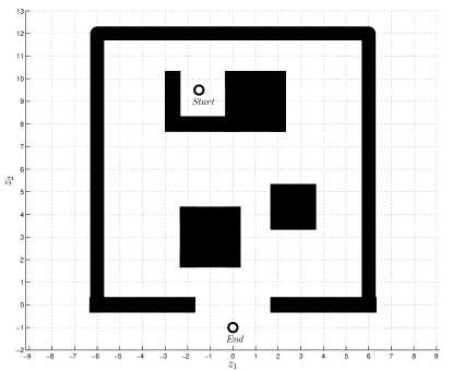
Figure 3: Map of area with obstacles

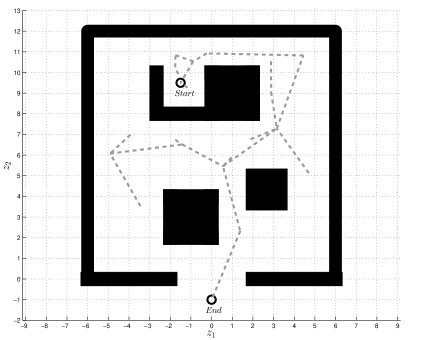
Figure 4: RRT used to identify the shortest path

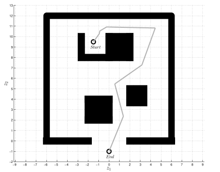
Figure 5: Shorted path extracted from the RRT

A collision avoidance system is now described based on the left inversion input formula for the bi-steerable car model developed in the previous section. The basic steps of the algorithm are as follows:

1. Map the area and obstacles where the bi-steerable car moves and provide a start location and an end location.

2. The RRT path planning algorithm described in [16] then uses the data from the previous step to compute the path between the start and end locations by first computing a tree and then identifying the shortest path within the tree from the start location to the end location.

3. The shortest path is then smoothed and approximated by a cubic spline.

4. Each spline section, which is a cubic polynomial, is fed to the left inversion formula in order to compute the corresponding control inputs $\bar{u}_{1}$ and $u_{2}$.

5. The inputs $\bar{u}_{1}$ and $u_{2}$ are finally used to drive the bi-steerable car.

Consider the following specific example:

i: Suppose the area with obstacles is the one shown in Figure 3. Pick the start and end locations to be:

$$Start: \;\;\;(-1.5,9.5)$$

$$End: \;\;\;(0,-1).$$

ii: The RRT generated for this map is shown in Figure 4. The shortest path between the given start and end locations exacted from this RRT is shown in Figure 5.

iii: The shortest path is then smoothed and approximated by cubic splines as shown in Figure 6. The constant terms of each cubic spline section must coincide with the final position of the previous section, This means that one does not need to fit the constant terms of the spline approximation. That is, the condition $(c,\emptyset)=(c_{y},\emptyset)$ in Theorem 1 is always satisfied by the cubic splines in the path approximations. The linear coefficient of the spline approximation is also subject to the range conditions of Theorem 1. However, since $z_{4}$ and $z_{5}$ in (26) are just the integrals of $u_{2}$ and $\bar{u}_{1}$, respectively, their corresponding initial conditions $z_{4,0}$ and $z_{5,0}$ can be chosen arbitrarily as long as $z_{5,0}\neq 0$, otherwise the decoupling matrix (27) is singular. Observe that

$$(c,x_{0})=\left(\begin{array}[]{c}z_{5,0}\cos(z_{3,0}+z_{4,0})\\ z_{5,0}\sin(z_{3,0}+z_{4,0})\end{array}\right),$$ (29)

where $z_{3,0}$ is known and fixed. Hence, one can always find $z_{4,0}$ and $z_{5,0}$ such that $(c,x_{0})$ matches the desired coefficient $(c_{y},x_{0})$, which comes from the spline approximation. Here the time interval for the simulation have been normalized to $[0,1]$ since only the kinematics are being considered.

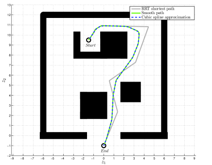
Figure 6: Shortest, smoothed and spline approximated paths

iv: The control inputs are now computed section by section. The first spline section has initial conditions

$$z_{1,0}=-1.5,\;\;z_{2,0}=9.5,\;\;z_{3,0}=1.5,$$

and the desired outputs of the path are

$$c_{y_{1}}=-1.5+10.75x_{0}-28.15x_{0}^{2}+185.15x_{0}^{3}$$

and

$$c_{y_{2}}=9.5+14.40x_{0}+13.07x_{0}^{2}-24.89x_{0}^{3}.$$

As expected, the constant coefficients are automatically equal to the start position of the car. Also, (29) is solved for $z_{4,0}$ and $z_{5,0}\neq 0$ so that $(c_{1},x_{0})=(c_{y_{1}},x_{0})=10.75$ and $(c_{2},x_{0})=(c_{y_{2}},x_{0})=14.40$, which gives

$$z_{4,0}=-4.00028,\;\;z_{5,0}=-17.97.$$

This solution is not unique. Since the overall time of the simulation was normalized, the time interval for each section of the path was chosen to have duration $t_{sim}=0.02$. The left inverse formulas in this case give

$$\bar{u}_{1}(t)= 7.74-195.52t+1592.16t^{2}+12925.9t^{3}$$

$$-443203.0t^{4}+4.26\times 10^{6}t^{5}+2.83\times 10^{6}t^{6}$$

and

$$u_{2}(t)= \,6.36-142.17t+386.62t^{2}-226.02t^{3}$$

$$-2648.52t^{4}+1280.47t^{5}+76475.8t^{6}.$$

Since the degree of the approximation was chosen to be $6$, these inputs give the following errors:

$$y_{1}(t)-\hat{y}_{1}(t)= {\;}1.33\times 10^{6}t^{7}-5.10\times 10^{6}t^{8}$$

$$-2.02\times 10^{7}t^{9}+3.47\times 10^{7}t^{10}+\cdots$$

and

$$y_{2}(t)-\hat{y}_{2}(t)= {\;}-1.24\times 10^{6}t^{7}+4.39\times 10^{6}t^{8}$$

$$+2.09\times 10^{7}t^{9}-2.82\times 10^{7}t^{10}+\cdots,$$

where $y_{i}$ is the $i$-th component of $y$ having generating series $c_{y}$, and $\hat{y}_{i}=c\circ c_{u}$ is truncated to degree $6$. The computed control inputs are shown in Figure 7.

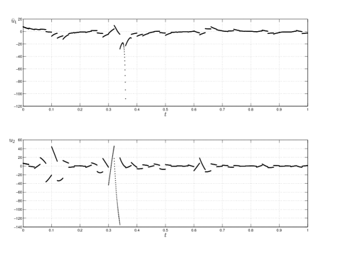
Figure 7: Control inputs $\bar{u}_{1}$ and $u_{2}$

iv: Finally, the computed control inputs $\bar{u}_{1}$ and $u_{2}$ are used to drive the bi-steerable car as shown in Figure 8. In the same figure, the bi-steerable car path is overlapped, as comparison, with the cubic spline approximation of the shortest path (avoiding obstacles) computed by the RRT algorithm. The degree of approximation and smoothness of the bi-steerable car path can be tuned by increasing or decreasing the number of partitions of the cubic spline approximation, and the degree of approximation of the computed left inverses. Tracking performance will ultimately be bounded by the amount of computational power available.

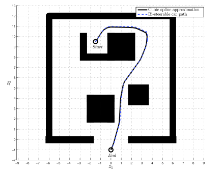
Figure 8: Cubic spline approximated path and bi-steerable car trajectory

V Conclusions

A collision avoidance system was described for a bi-steerable car based on a left inversion formula for Fliess operators whose generating series have a well defined vector relative degree. This allows one to integrate directly the kinematics of the car and a path planning algorithm without the need for passing through a flat output as is done in other methods. In principle, the full dynamics could also be inverted to give a more realistic collision avoidance system. The method was demonstrated by numerical simulation.

References

- [1] A. de Luca, G. Oriolo, and M. Vendittelli, Control of wheeled mobile robots. Experimental overview, in RAMSETE: Articulated and Mobile Robots for SErvices and TEchnologies, S. Nicosia, B. Siciliano, A. Bicchi, and P. Valigi, Eds., Springer, London, 2001, pp. 181–226.
- [2] L. A. Duffaut Espinosa, K. Ebrahimi-Fard, and W. S. Gray, A combinatorial Hopf algebra for nonlinear output feedback control systems, Journal of Algebra, 453 (2016) 609–643.
- [3] H. W. Engl and P. Kügler, Nonlinear inverse problems: Theoretical aspects and some industrial applications, in Multidisciplinary Methods for Analysis, Optimization and Control of Complex Systems, V. Capasso and J. Periaux, Eds., Springer, Heidelberg, 2005 pp. 3–48.
- [4] M. Fliess, J. Lévine, P. Martine and P. Rouchon, Flatness and defect of non-linear systems: introductory theory and examples, International Journal of Control, 61 (1995) 1327–1361.
- [5] N. H. Getz, Dynamic Inversion of Nonlinear Maps with Applications to Nonlinear Control and Robotics, Ph.D. dissertation, UC Berkeley, Berkeley, CA, 1996.
- [6] W. S. Gray, L. A. Duffaut Espinosa, and K. Ebrahimi-Fard, Recursive algorithm for the antipode in the SISO feedback product, Proc. 21st Inter. Symp. on the Mathematical Theory of Networks and Systems, Groningen, The Netherlands, 2014, pp. 1088–1093.
- [7] , Analytic left inversion of multivariable Lotka-Volterra models, Proc. 54th IEEE Conf. on Decision and Control, Osaka, Japan, 2015, pp. 6472–6477.
- [8] , Faà di Bruno Hopf algebra of the output feedback group for multivariable Fliess Operators, Systems & Control Letters, 74 (2014) 64–73.
- [9] W. S. Gray, L. A. Duffaut Espinosa, and M. Thitsa, Left inversion of analytic nonlinear SISO systems via formal power series methods, Automatica, 50 (2014) 2381–2388.
- [10] A. Hars, Autonomous cars: The next revolution looms, Inventivio Innovation Briefs 2010-01, Nuremberg, 2010, www.inventivio.com/innovationbriefs/2010-01.
- [11] J. Hermosillo, C. Pradalier, S. Sekhavat, C. Laugier, and G. Baille, Towards motion autonomy of a bi-steerable car: Experimental issues from map-building to trajectory execution, Proc. 2003 IEEE Inter. Conf. on Robotics & Automation, Taipei, Taiwan, 2003.
- [12] J. Hermosillo and S. Sekhavat, Feedback control of a bi-steerable car using flatness application to trajectory tracking, Proc. 2003 ACC, Denver, CO, 2003, pp. 3567–3572.
- [13] R. M. Hirschorn, Invertibility of nonlinear control systems, SIAM Journal on Control and Optimization, 17 (1979) 289–297.
- [14] , Invertibility of multivariable nonlinear control systems, IEEE Transactions on Automatic Control, AC-24 (1979) 855–865.
- [15] A. Isidori, Nonlinear Control Systems, 3rd Ed., Springer-Verlag, London, 1995.
- [16] S. LaValle, Planning Algorithms, Cambridge University Press, New York, 2006.
- [17] J. Lévine, Analysis and Control of Nonlinear Systems: A Flatness-based Approach, Springer, Berlin, 2009.
- [18] Wolfram Research, Inc., Mathematica, Version 10.0, Champaign, IL, 2014.
- [19] P. Petrov, Nonlinear path following control for a bi-steerable vehicle, Information Technologies and Control, 1 (2009) 14–19.
- [20] S. Sekhavat and J. Hermosillo, Cycab bi-steerable cars: a new family of differentially flat systems, Advanced Robotics, 16 (2002) 445–462.
- [21] S. Sekhavat, J. Hermosillo, and P. Rouchon, Motion planning for a bi-Steerable car, Proc. 2001 IEEE Inter. Conf. on Robotics & Automation, Seoul, South Korea, 2001, pp. 3294–3299.
- [22] S. Sekhavat, P. Rouchon, and J. Hermosillo, Computing the flat outputs of Engel differential systems, the case study of the bi-steerable car, Proc. 2001 ACC, Arlington, VA, 2001, pp. 3576–3581.
- [23] S. N. Singh, A modified algorithm for invertibility in nonlinear systems, IEEE Transactions on Automatic Control, AC-26 (1981) 595–598.
- [24] , Invertibility of observable multivariable nonlinear systems, IEEE Transaction on Automatic Control, AC-27 (1981) 487–489.
- [25] S. A. Tchenderli-Braham and F. Hamerlain, Trajectory tracking with a hybrid control applied to a bi-steerable car, Proc. 2nd Inter. Conf. on Systems and Computer Science Villeneuve d’Ascq, France, 2013, pp. 252–256.
- [26] Y. Wang, Differential Equations and Nonlinear Control Systems, Ph.D. dissertation, Rutgers University, New Brunswick, NJ, 1990.
- [27] I. M. Winter-Arboleda, W. S. Gray, and L. A. Duffaut Espinosa, Expanding the class of globally convergent Fliess operators, Proc. 22nd Inter. Symp. on the Mathematical Theory of Networks and Systems, Minneapolis, USA, 2016, under review.