Fast Incremental Method for Nonconvex Optimization

Abstract

We analyze a fast incremental aggregated gradient method for optimizing nonconvex problems of the form $\min_{x}\sum_{i}f_{i}(x)$. Specifically, we analyze the Saga algorithm within an Incremental First-order Oracle framework, and show that it converges to a stationary point provably faster than both gradient descent and stochastic gradient descent. We also discuss a Polyak’s special class of nonconvex problems for which Saga converges at a linear rate to the global optimum. Finally, we analyze the practically valuable regularized and minibatch variants of Saga. To our knowledge, this paper presents the first analysis of fast convergence for an incremental aggregated gradient method for nonconvex problems.

1 Introduction

We study the finite-sum optimization problem

$$\min_{x\in\mathbb{R}^{d}}\ f(x):=\frac{1}{n}\sum_{i=1}^{n}f_{i}(x),$$ (1)

where each $f_{i}$ ($i\in\{1,\dots,n\}\triangleq[n]$) can be nonconvex; our only assumption is that the gradients of $f_{i}$ exist and are Lipschitz continuous. We denote the class of such instances of (1) by $\mathcal{F}_{n}$.

Problems of the form (1) are of central importance in machine learning where they occur as instances of empirical risk minimization; well-known examples include logistic regression (convex) James et al. (2013) and deep neural networks (nonconvex) Deng & Yu (2014). Consequently, such problems have been intensively studied. A basic approach for solving (1) is gradient descent (GradDescent), described by the following update rule:

$$x^{t+1}=x^{t}-\eta_{t}\nabla f(x^{t}),\text{ where }\eta_{t}>0.$$ (2)

However, iteration (2) is prohibitively expensive in large-scale settings where $n$ is very large. For such settings, stochastic and incremental methods are typical Bertsekas (2011); Defazio et al. (2014). These methods use cheap noisy estimates of the gradient at each iteration of (2) instead of $\nabla f(x^{t})$. A particularly popular approach, stochastic gradient descent (Sgd) uses $\nabla f_{i_{t}}$, where $i_{t}$ in chosen uniformly randomly from $\{1,\dots,n\}$. While the cost of each iteration is now greatly reduced, it is not without any drawbacks. Due to the noise (also known as variance in stochastic methods) in the gradients, one has to typically use decreasing step-sizes $\eta_{t}$ to ensure convergence, and consequently, the convergence rate gets adversely affected.

Therefore, it is of great interest to overcome the slowdown of Sgd without giving up its scalability. Towards this end, for convex instances of (1), remarkable progress has been made recently. The key realization is that if we make multiple passes through the data, we can store information that allows us to reduce variance of the stochastic gradients. As a result, we can use constant stepsizes (rather than diminishing scalars) and obtain convergence faster than Sgd, both in theory and practice Johnson & Zhang (2013); Schmidt et al. (2013); Defazio et al. (2014).

Nonconvex instances of (1) are also known to enjoy similar speedups Johnson & Zhang (2013), but existing analysis does not explain this success as it relies heavily on convexity to control variance. Since Sgd dominates large-scale nonconvex optimization (including neural network training), it is of great value to develop and analyze faster nonconvex stochastic methods.

With the above motivation, we analyze Saga Defazio et al. (2014), an incremental aggregated gradient algorithm that extends the seminal Sag method of Schmidt et al. (2013), and has been shown to work well for convex finite-sum problems Defazio et al. (2014). Specifically, we analyze Saga for the class $\mathcal{F}_{n}$ using the incremental first-order oracle (IFO) framework Agarwal & Bottou (2014). For $f\in\mathcal{F}_{n}$, an IFO is a subroutine that takes an index $i\in[n]$ and a point $x\in\mathbb{R}^{d}$, and returns the pair $(f_{i}(x),\nabla f_{i}(x))$.

To our knowledge, this paper presents the first analysis of fast convergence for an incremental aggregated gradient method for nonconvex problems. The attained rates improve over both Sgd and GradDescent, a benefit that is also corroborated by experiments. Before presenting our new analysis, let us briefly recall some items of related work.

1.1 Related work

A concise survey of incremental gradient methods is Bertsekas (2011). An accessible analysis of stochastic convex optimization ($\min\mathbb{E}_{z}[F(x,z)]$) is Nemirovski et al. (2009). Classically, Sgd stems from the seminal work Robbins & Monro (1951), and has since witnessed many developments Kushner & Clark (2012), including parallel and distributed variants Bertsekas & Tsitsiklis (1989); Agarwal & Duchi (2011); Recht et al. (2011), though non-asymptotic convergence analysis is limited to convex setups. Faster rates for convex problems in $\mathcal{F}_{n}$ are attained by variance reduced stochastic methods, e.g., Defazio et al. (2014); Johnson & Zhang (2013); Schmidt et al. (2013); Shalev-Shwartz & Zhang (2013); Reddi et al. (2015). Linear convergence of stochastic dual coordinate ascent when $f_{i}$ ($i\in[n]$) may be nonconvex but $f$ is strongly convex is studied in Shalev-Shwartz (2015). Lower bounds for convex finite-sum problems are studied in Agarwal & Bottou (2014).

For nonconvex nonsmooth problems the first incremental proximal-splitting methods is in Sra (2012), though only asymptotic convergence is studied. Hong Hong (2014) studies convergence of a distributed nonconvex incremental ADMM algorithm. The first work to present non-asymptotic convergence rates for Sgd is Ghadimi & Lan (2013); this work presents an $O(1/\epsilon^{2})$ iteration bound for Sgd to satisfy approximate stationarity $\|\nabla f(x)\|^{2}\leq\epsilon$, and their convergence criterion is motivated by the gradient descent analysis of Nesterov Nesterov (2003). The first analysis for nonconvex variance reduced stochastic gradient is due to Shamir (2014), who apply it to the specific problem of principal component analysis (PCA).

2 Preliminaries

In this section, we further explain our assumptions and goals. We say $f$ is $L$-smooth if there is a constant $L$ such that

$$\|\nabla f(x)-\nabla f(y)\|\leq L\|x-y\|,\quad\forall\ x,y\in\mathbb{R}^{d}.$$

Throughout, we assume that all $f_{i}$ in (1) are $L$-smooth, i.e., $\|\nabla f_{i}(x)-\nabla f_{i}(y)\|\leq L\|x-y\|$ for all $i\in[n]$. Such an assumption is common in the analysis of first-order methods. For ease of exposition, we assume the Lipschitz constant $L$ to be independent of $n$. For our analysis, we also discuss the class of $\tau$-gradient dominated Polyak (1963); Nesterov & Polyak (2006) functions, namely functions for which

$$f(x)-f(x^{*})\leq\tau\|\nabla f(x)\|^{2},$$ (3)

where $x^{*}$ is a global minimizer of $f$. This class of functions was originally introduced by Polyak in Polyak (1963). Observe that such functions need not be convex. Also notice that gradient dominance (3) is a restriction on the overall function $f$, but not on the individual functions $f_{i}$ ($i\in[n]$).

Following Nesterov (2003); Ghadimi & Lan (2013) we use $\|\nabla f(x)\|^{2}\leq\epsilon$ to judge approximate stationarity of $x$. Contrast this with Sgd for convex $f$, where one uses $[f(x)-f(x^{*})]$ or $\|x-x^{*}\|^{2}$ as criteria for convergence analysis. Such criteria cannot be used for nonconvex functions due to the intractability of the problem.

While the quantities $\|\nabla f(x)\|^{2}$, $[f(x)-f(x^{*})]$, or $\|x-x^{*}\|^{2}$ are not comparable in general, they are typically assumed to be of similar magnitude (see Ghadimi & Lan (2013)). We note that our analysis does not assume $n$ to be a constant, so we report dependence on it in our results. Furthermore, while stating our complexity results, we assume that the initial point of the algorithms is constant, i.e., $f(x^{0})-f(x^{*})$ and $\|x^{0}-x^{*}\|$ are constants. For our analysis, we will need the following definition.

Definition 1.

A point $x$ is called $\epsilon$-accurate if $\|\nabla f(x)\|^{2}\leq\epsilon$. A stochastic iterative algorithm is said to achieve $\epsilon$-accuracy in $t$ iterations if $\mathbb{E}[\|\nabla f(x^{t})\|^{2}]\leq\epsilon$, where the expectation is taken over its stochasticity.

We start our discussion of algorithms by recalling Sgd, which performs the following update in its $t^{\text{th}}$ iteration:

$$x^{t+1}=x^{t}-\eta_{t}\nabla f_{i_{t}}(x),$$ (4)

where $i_{t}$ is a random index chosen from $[n]$, and the gradient $\nabla f_{i_{t}}(x^{t})$ approximates the gradient of $f$ at $x^{t}$, $\nabla f(x^{t})$. It can be seen that the update is unbiased, i.e., $\mathbb{E}[\nabla f_{i_{t}}(x^{t})]=\nabla f(x^{t})$ since the index $i_{t}$ is chosen uniformly at random. Though the Sgd update is unbiased, it suffers from variance due to the aforementioned stochasticity in the chosen index. To control the variance one has to decrease the step size $\eta_{t}$ in (4), which in turn leads to slow convergence. The following is a well-known result on Sgd in the context of nonconvex optimization Ghadimi & Lan (2013).

Theorem 1.

Suppose $\|\nabla f_{i}\|\leq\sigma$ i.e., gradient of function $f_{i}$ is bounded for all $i\in[n]$, then the IFO complexity of Sgd to obtain an $\epsilon$-accurate solution is $O(1/\epsilon^{2})$.

It is instructive to compare the above result with the convergence rate of GradDescent. The IFO complexity of GradDescent is $O(n/\epsilon)$. Thus, while Sgd eliminates the dependence on $n$, the convergence rate worsens to $O(1/\epsilon^{2})$ from $O(1/\epsilon)$ in GradDescent. In the next section, we investigate an incremental method with faster convergence.

3 Algorithm

We describe below the Saga algorithm and prove its fast convergence for nonconvex optimization. Saga is a popular incremental method in machine learning and optimization communities. It is very effective in reducing the variance introduced due to stochasticity in Sgd. Algorithm 1 presents pseudocode for Saga. Note that the update $v^{t}$ (Line 5) is unbiased, i.e., $\mathbb{E}[v^{t}]=\nabla f(x^{t})$. This is due to the uniform random selection of index $i_{t}$. It can be seen in Algorithm 1 that Saga maintains gradients at $\alpha_{i}$ for $i\in[n]$. This additional set is critical to reducing the variance of the update $v^{t}$. At each iteration of the algorithm, one of the $\alpha_{i}$ is updated to the current iterate. An implementation of Saga requires storage and updating of gradients $\nabla f_{i}(\alpha_{i})$; the storage cost of the algorithm is $nd$. While this leads to higher storage in comparison to Sgd, this cost is often reasonable for many applications. Furthermore, this cost can be reduced in the case of specific models; refer to Defazio et al. (2014) for more details.

For ease of exposition, we introduce the following quantity:

$$\Gamma_{t}=\bigl{(}\eta-\tfrac{c_{t+1}\eta}{\beta}-\eta^{2}L-2c_{t+1}\eta^{2}\bigr{)},$$ (5)

where the parameters $c_{t+1}$, $\beta$ and $\eta$ will be defined shortly. We start with the following set of key results that provide convergence rate of Algorithm 1.

Algorithm 1 SAGA$\left(x^{0},T,\eta\right)$

1:  Input: $x^{0}\in\mathbb{R}^{d}$, $\alpha_{i}^{0}=x^{0}$ for $i\in[n]$, number of iterations $T$, step size $\eta>0$

2:  $g^{0}=\frac{1}{n}\sum_{i=1}^{n}\nabla f_{i}(\alpha_{i}^{0})$

3:  for $t=0$ to $T-1$ do

4:     Uniformly randomly pick $i_{t},j_{t}$ from $[n]$

5:     $v^{t}=\nabla f_{i_{t}}(x^{t})-\nabla f_{i_{t}}(\alpha_{i_{t}}^{t})+g^{t}$

6:     $x^{t+1}=x^{t}-\eta v^{t}$

7:     $\alpha_{j_{t}}^{t+1}=x^{t}$ and $\alpha_{j}^{t+1}=\alpha_{j}^{t}$ for $j\neq j_{t}$

8:     $g^{t+1}=g^{t}-\frac{1}{n}(\nabla f_{j_{t}}(\alpha_{j_{t}}^{t})-\nabla f_{j_{t}}(\alpha_{j_{t}}^{t+1}))$

9:  end for

10:  Output: Iterate $x_{a}$ chosen uniformly random from $\{x^{t}\}_{t=0}^{T-1}$.

Lemma 1.

For $c_{t},c_{t+1},\beta>0$, suppose we have

$$c_{t}=c_{t+1}(1-\tfrac{1}{n}+\eta\beta+2\eta^{2}L^{2})+\eta^{2}L^{3}.$$

Also let $\eta$, $\beta$ and $c_{t+1}$ be chosen such that $\Gamma_{t}>0$. Then, the iterates $\{x^{t}\}$ of Algorithm 1 satisfy the bound

$$\mathbb{E}[\|\nabla f(x^{t})\|^{2}]\leq\frac{R^{t}-R^{t+1}}{\Gamma_{t}},$$

where $R^{t}:=\mathbb{E}[f(x^{t})+(c_{t}/n)\sum_{i=1}^{n}\|x^{t}-\alpha_{i}^{t}\|^{2}]$.

The proof of this lemma is given in Section 9. Using this lemma we prove the following result on the iterates of Saga.

Theorem 2.

Let $f\in\mathcal{F}_{n}$. Let $c_{T}=0$, $\beta>0$, and $c_{t}=c_{t+1}(1-\tfrac{1}{n}+\eta\beta+2\eta^{2}L^{2})+\eta^{2}L^{3}$ be such that $\Gamma_{t}>0$ for $0{\;\leq\;}t{\;\leq\;}T-1$. Define the quantity $\gamma_{n}:=\min_{0\leq t\leq T-1}\Gamma_{t}$. Then the output $x_{a}$ of Algorithm 1 satisfies the bound

$$\mathbb{E}[\|\nabla f(x_{a})\|^{2}]\leq\frac{f(x^{0})-f(x^{*})}{T\gamma_{n}},$$

where $x^{*}$ is an optimal solution to (1).

Proof.

We apply telescoping sums to the result of Lemma 1 to obtain

$$\gamma_{n}\sum\nolimits_{t=0}^{T-1}\mathbb{E}[\|\nabla f(x^{t})\|^{2}] \leq\sum\nolimits_{t=0}^{T-1}\Gamma_{t}\mathbb{E}[\|\nabla f(x^{t})\|^{2}]$$

$$\leq R^{0}-R^{T}.$$

The first inequality follows from the definition of $\gamma_{n}$. This inequality in turn implies the bound

$$\sum\nolimits_{t=0}^{T-1}\mathbb{E}[\|\nabla f(x^{t})\|^{2}]\leq\frac{\mathbb{E}[f(x^{0})-f(x^{T})]}{\gamma_{n}},$$ (6)

where we used that $R^{T}=\mathbb{E}[f(x^{T})]$ (since $c_{T}=0$), and that $R^{0}=\mathbb{E}[f(x^{0})]$ (since $\alpha_{i}^{0}=x^{0}$ for $i\in[n]$). Using inequality (6), the optimality of $x^{*}$, and the definition of $x_{a}$ in Algorithm 1, we obtain the desired result. ∎

Note that the notation $\gamma_{n}$ involves $n$, since this quantity can depend on $n$. To obtain an explicit dependence on $n$, we have to use an appropriate choice of $\beta$ and $\eta$. This is made precise by the following main result of the paper.

Theorem 3.

Suppose $f\in\mathcal{F}_{n}$. Let $\eta=1/(3Ln^{2/3})$ and $\beta=L/n^{1/3}$. Then, $\gamma_{n}\geq\frac{1}{12Ln^{2/3}}$ and we have the bound

$$\mathbb{E}[\|\nabla f(x_{a})\|^{2}] \leq\frac{12Ln^{2/3}[f(x^{0})-f(x^{*})]}{T},$$

where $x^{*}$ is an optimal solution to the problem in (1) and $x_{a}$ is the output of Algorithm 1.

Proof.

With the values of $\eta$ and $\beta$, let us first establish an upper bound on $c_{t}$. Let $\theta$ denote $\tfrac{1}{n}-\eta\beta-2\eta^{2}L^{2}$. Observe that $\theta<1$ and $\theta\geq 4/(9n)$. This is due to the specific values of $\eta$ and $\beta$ stated in the theorem. Also, we have $c_{t}=c_{t+1}(1-\theta)+\eta^{2}L^{3}$. Using this relationship, it is easy to see that $c_{t}=\eta^{2}L^{3}\tfrac{1-(1-\theta)^{T-t}}{\theta}$. Therefore, we obtain the bound

$$c_{t}=\eta^{2}L^{3}\tfrac{1-(1-\theta)^{T-t}}{\theta}\leq\frac{\eta^{2}L^{3}}{\theta}\leq\frac{L}{4n^{1/3}},$$ (7)

for all $0\leq t\leq T$, where the inequality follows from the definition of $\eta$ and the fact that $\theta\geq 4/(9n)$. Using the above upper bound on $c_{t}$ we can conclude that

$$\gamma_{n} =\min_{t}\bigl{(}\eta-\tfrac{c_{t+1}\eta}{\beta}-\eta^{2}L-2c_{t+1}\eta^{2}\bigr{)}\geq\frac{1}{12Ln^{2/3}},$$

upon using the following inequalities: (i) $c_{t+1}\eta/\beta\leq\eta/4$, (ii) $\eta^{2}L\leq\eta/3$ and (iii) $2c_{t+1}\eta^{2}\leq\eta/6$, which hold due to the upper bound on $c_{t}$ in (7). Substituting this bound on $\gamma_{n}$ in Theorem 2, we obtain the desired result. ∎

A more general result with step size $\eta<1/(3Ln^{2/3})$ can be proved, but it will only lead to a theoretically suboptimal convergence result. Recall that each iteration of Algorithm 1 requires $O(1)$ IFO calls. Using this fact, we can rewrite Theorem 3 in terms of its IFO complexity as follows.

Corollary 1.

If $f\in\mathcal{F}_{n}$, then the IFO complexity of Algorithm 1 (with parameters from Theorem 3) to obtain an $\epsilon$-accurate solution is $O(n+n^{2/3}/\epsilon)$.

This corollary follows from the $O(1)$ per iteration cost of Algorithm 1 and because $n$ IFO calls are required to calculate $g^{0}$ at the start of the algorithm. In special cases, the initial $O(n)$ IFO calls can be avoided (refer to Schmidt et al. (2013); Defazio et al. (2014) for details). By comparing the IFO complexity of Saga ($O(n+n^{2/3}/\epsilon)$) with that of GradDescent ($O(n/\epsilon)$), we see that Saga is faster than GradDescent by a factor of $n^{1/3}$.

4 Finite Sums with Regularization

In this section, we study the problem of finite-sum problems with additional regularization. More specifically, we consider problems of the form

$$\min_{x\in\mathbb{R}^{d}}\ f(x):=\frac{1}{n}\sum_{i=1}^{n}f_{i}(x)+r(x),$$ (8)

where $r:\mathbb{R}^{d}\rightarrow\mathbb{R}$ is an $L$-smooth (possibly nonconvex) function. Problems of this nature arise in machine learning where the functions $f_{i}$ are loss functions and $r$ is a regularizer. Since we assumed $r$ to be smooth, (8) can be reformulated as (1) by simply encapsulating $r$ into the functions $f_{i}$. However, as we will see, it is beneficial to handle the regularization separately. We call the variant of Saga with the additional regularization as Reg-Saga. The key difference between Reg-Saga and Saga lies in Line 6 of Algorithm 1. In particular, for Reg-Saga, Line 6 of Algorithm 1 is replaced with the following update:

$$x^{t+1}=x^{t}-\eta(v^{t}+\nabla r(x^{t})).$$ (9)

Note that the primary difference is that the part of gradient based on function $r$ is updated at each iteration of the algorithm. The convergence of Reg-Saga can be proved along the lines of our analysis of Saga. Hence, we omit the details for brevity and directly state the following key result stating the IFO complexity of Reg-Saga.

Theorem 4.

If function $f$ is of the form in (8), then the IFO complexity of Reg-Saga to obtain an $\epsilon$-accurate solution is $O(n+n^{2/3}/\epsilon)$.

The proof essentially follows along the lines of the proof of Theorem 3. The difference, however, being that the update corresponding to function $r(x)$ is handled explicitly at each iteration. Note that the above IFO complexity is not different from that in Corollary 1. However, its main benefit comes in the form of storage efficiency in problems with more structure. To understand this, consider the problems of form

$$\min_{x\in\mathbb{R}^{d}}\ f(x):=\frac{1}{n}\sum_{i=1}^{n}l(x^{\top}z_{i})+r(x),$$ (10)

where $z_{i}\in\mathbb{R}^{d}$ for $i\in[n]$ while $l:\mathbb{R}\rightarrow\mathbb{R}_{\geq 0}$ is a differentiable loss function. Here, $l$ and $r$ can be in general nonconvex. Such problems are popularly known as (regularized) empirical risk minimization in machine learning literature. We can directly apply Saga to (10) by casting it in the form (1). However, recall that the storage cost of Saga is $O(nd)$ due to the cost of storing the gradient at $\alpha_{i}^{t}$. This storage cost can be avoided in Reg-Saga by handling the function $r$ separately. Indeed, for Reg-Saga we need to store just $\nabla l(x^{\top}z_{i})$ for all $i\in[n]$ (as $\nabla r(x)$ is updated at each iteration). By observing that $\nabla l(x^{\top}z_{i})=l^{\prime}(x^{\top}z_{i})z_{i}$, where $l^{\prime}$ represents the derivative of $l$, it is apparent that we need to store only the scalars $l^{\prime}(x^{\top}z_{i})$ for Reg-Saga. This reduces the storage $O(n)$ instead of $O(nd)$ in Saga.

5 Linear convergence rates for gradient dominated functions

Until now the only assumption we used was Lipschitz continuity of gradients. An immediate question is whether the IFO complexity can be further improved under stronger assumptions. We provide an affirmative answer to this question by showing that for gradient dominated functions, a variant of Saga attains linear convergence rate. Recall that a function $f$ is called $\tau$-gradient dominated if around an optimal point $x^{*}$, $f$ satisfies the following growth condition:

$$f(x)-f(x^{*})\leq\tau\|\nabla f(x)\|^{2},\quad\forall x\in\mathbb{R}^{d}.$$

For such functions, we use the variant of Saga shown in Algorithm 2. Observe that Algorithm 2 uses Saga as a subroutine. Alternatively, one can rewrite Algorithm 2 in the form of $KT$ iterations of Algorithm 1 where one updates $\{\alpha_{i}\}$ after every $T$ iterations and then selects a random iterate amongst the last $T$ iterates. For this variant of Saga, we can prove the following linear convergence result.

Algorithm 2 GD-SAGA$\left(x^{0},K,T,\eta\right)$

  Input: $x^{0}\in\mathbb{R}^{d}$, $K$, epoch length $m$, step sizes $\eta>0$

  for $k=0$ to $K$ do

     $x^{k}=\text{SAGA}(x^{k-1},T,\eta)$

  end for

  Output: $x^{K}$

Theorem 5.

If $f$ is $\tau$-gradient dominated, then with $\eta=1/(3Ln^{2/3})$ and $T=\lceil 24L\tau n^{2/3}\rceil$, the iterates of Algorithm 2 satisfy $\mathbb{E}[\|f(x^{k})\|^{2}]\leq 2^{-k}\|f(x^{0})\|^{2},$ where $x^{*}$ is an optimal solution of (1).

Proof.

The iterates of Algorithm 2 satisfy the bound

$$\mathbb{E}[\|\nabla f(x^{k})\|^{2}]\leq\frac{\mathbb{E}[f(x^{k-1})-f(x^{*})]}{2\tau},$$ (11)

which holds due to Theorem 3 given the choices of $\eta$ and $T$ assumed in the statement. However, $f$ is $\tau$-gradient dominated, so $\mathbb{E}[\|\nabla f(x^{k-1})\|^{2}]\geq\mathbb{E}[f(x^{k-1})-f(x^{*})]/\tau$, which combined with (11) concludes the proof. ∎

An immediate consequence of this theorem is the following.

Corollary 2.

If $f$ is $\tau$-gradient dominated, the IFO complexity of Algorithm 2 (with parameters from Theorem 5) to compute an $\epsilon$-accurate solution is $O((n+\tau n^{2/3})\log(1/\epsilon))$.

While we state the result in terms of $\|\nabla f(x)\|^{2}$, it is not hard to see that for gradient dominated functions a similar result holds for the convergence criterion being $[f(x)-f(x^{*})]$.

Theorem 6.

If $f$ is $\tau$-gradient dominated, with $\eta=1/(3Ln^{2/3})$ and $T=\lceil 24L\tau n^{2/3}\rceil$, the iterates of Algorithm 2 satisfy

$$\mathbb{E}[f(x^{k})-f(x^{*})]\leq 2^{-k}[f(x^{0})-f(x^{*})],$$

where $x^{*}$ is an optimal solution to (1).

A noteworthy aspect of the above result is the linear convergence rate to a global optimum. Therefore, the above result is stronger than Theorem 3. Note that throughout our analysis of gradient dominated functions, no assumptions other than Lipschitz smoothness are placed on the individual set of functions $f_{i}$. We emphasize here that these results can be further improved with additional assumptions (e.g., strong convexity) on the individual functions $f_{i}$ and on $f$. Also note that GradDescent can achieve linear convergence rate for gradient dominated functions Polyak (1963). However, the IFO complexity of GradDescent is $O(\tau n\log(1/\epsilon))$, which is strictly worse than IFO complexity of GD-Saga (see Corollary 2).

6 Minibatch Variant

A common variant of incremental methods is to sample a set of indices $I_{t}$ instead of single index $i_{t}$ when approximating the gradient. Such a variant is generally referred to as a “minibatch” version of the algorithm. Minibatch variants are of great practical significance since they reduce the variance of incremental methods and promote parallelism. Algorithm 3 lists the pseudocode for a minibatch variant of Saga. Algorithm 3 uses a set $I_{t}$ of size $|I_{t}|=b$ for calculating the update $v^{t}$ instead of a single index $i_{t}$ used in Algorithm 1. By using a larger $b$, one can reduce the variance due to the stochasticity in the algorithm. Such a procedure is also beneficial in parallel settings since the calculation of the update $v^{t}$ can be parallelized. For this algorithm, we can prove the following convergence result.

Theorem 7.

Suppose $f\in\mathcal{F}_{n}$. Let $\eta=b/(3Ln^{2/3})$ and $\beta=L/n^{1/3}$. Then for the output $x_{a}$ of Algorithm 3 (with $b<n^{2/3}$) we have $\gamma_{n}\geq\frac{b}{12Ln^{2/3}}$ and

$$\mathbb{E}[\|\nabla f(x_{a})\|^{2}] \leq\frac{12Ln^{2/3}[f(x^{0})-f(x^{*})]}{bT},$$

where $x^{*}$ is an optimal solution to (1).

We omit the details of the proof since it is similar to the proof of Theorem 3. Note that the key difference in comparison to Theorem 1 is that we can now use a more aggressive step size $\eta=b/(3Ln^{2/3})$ due to a larger minibatch size $b$. An interesting aspect of the result is the $O(1/b)$ dependence on the minibatch size $b$. As long as this size is not large ($b<n^{2/3}$), one can significantly improve the convergence rate to a stationary point. A restatement of aforementioned result in terms of IFO complexity is provided below.

Corollary 3.

If $f\in\mathcal{F}_{n}$, then the IFO complexity of Algorithm 3 (with parameters from Theorem 7 and minibatch size $b<n^{2/3}$) to obtain an $\epsilon$-accurate solution is $O(n+n^{2/3}/\epsilon)$.

Algorithm 3 Minibatch-SAGA$\left(x^{0},b,T,\eta\right)$

1:  Input: $x^{0}\in\mathbb{R}^{d}$, $\alpha_{i}^{0}=x^{0}$ for $i\in[n]$, minibatch size $b$, number of iterations $T$, step size $\eta>0$

2:  $g^{0}=\frac{1}{n}\sum_{i=1}^{n}\nabla f_{i}(\alpha_{i}^{0})$

3:  for $t=0$ to $T-1$ do

4:     Uniformly randomly pick (with replacement) indices sets $I_{t},J_{t}$ of size $b$ from $[n]$

5:     $v^{t}=\frac{1}{|I_{t}|}\sum_{i\in I_{t}}(\nabla f_{i}(x^{t})-\nabla f_{i}(\alpha_{i_{t}}^{t}))+g^{t}$

6:     $x^{t+1}=x^{t}-\eta v^{t}$

7:     $\alpha_{j}^{t+1}=x^{t}$ for $j\in J_{t}$ and $\alpha_{j}^{t+1}=\alpha_{j}^{t}$ for $j\notin J_{t}$

8:     $g^{t+1}=g^{t}-\frac{1}{n}\sum_{j\in J_{t}}(\nabla f_{j}(\alpha_{j}^{t})-\nabla f_{j}(\alpha_{j}^{t+1}))$

9:  end for

10:  Output: Iterate $x_{a}$ chosen uniformly random from $\{x^{t}\}_{t=0}^{T-1}$.

By comparing the above result with Corollary 1, we can see that the IFO complexity of minibatch-Saga is the same Saga. However, since the $b$ gradients can be computed in parallel, one can achieve (theoretical) $b$ times speedup in multicore and distributed settings. In contrast, the performance Sgd degrades with minibatch size $b$ since the improvement in convergence rate for Sgd is typically $O(1/\sqrt{b})$ but $b$ IFO calls are required at each iteration of minibatch-Sgd. Thus, Saga has a much more efficient minibatch version in comparison to Sgd.

Discussion of Convergence Rates

Before ending our discussion on convergence rates, it is important to compare and contrast different convergence rates obtained in the paper. For general smooth nonconvex problems, we observed that Saga has a low IFO complexity of $O(n+n^{2/3}/\epsilon)$ in comparison to Sgd ($O(1/\epsilon^{2})$) and GradDescent ($O(n/\epsilon)$). This difference in the convergence is especially significant if one requires a medium to high accuracy solution, i.e., $\epsilon$ is small.

Furthermore, for gradient dominated functions, where Sgd obtains a sublinear convergence rate of $O(1/\epsilon^{2})$ as opposed to fast linear convergence rate of a variant of Saga (see Theorem 2). It is an interesting future work to explore other setups where we can achieve stronger convergence rates.

From our analysis of minibatch-Saga in Section 6, we observe that Saga profits from mini-batching much more than Sgd. In particular, one can achieve a (theoretical) linear speedup using mini-batching in Saga in parallel settings. On the other hand, the performance of Sgd typically degrades with minibatching. In summary, Saga enjoys all the benefits of GradDescent like constant step size, efficient minibatching with much weaker dependence on $n$.

Notably, Saga, unlike Sgd, does not use any additional assumption of bounded gradients (see Theorem 1 and Corollary 1). Moreover, if one uses a constant step size for Sgd, we need to have an advance knowledge of the total number of iterations $T$ in order to obtain the convergence rate mentioned in Theorem 1.

7 Experiments

We present our empirical results in this section. For our experiments, we study the problem of binary classification using nonconvex regularizers. The input consists of tuples $\{(z_{i},y_{i})\}_{i=1}^{n}$ where $z_{i}\in\mathbb{R}^{d}$ (commonly referred to as features) and $y_{i}\in\{-1,1\}$ (class labels). We are interested in the empirical loss minimization setup described in Section 4. Recall that problem of finite sum with regularization takes the form

$$\min_{x\in\mathbb{R}^{d}}\ f(x):=\frac{1}{n}\sum_{i=1}^{n}f_{i}(x)+r(x).$$ (12)

For our experiments, we use logistic function for $f_{i}$, i.e., $f_{i}(x)=\log(1+\exp(-y_{i}x^{\top}z_{i}))$ for all $i\in[n]$. All $z_{i}$ are normalized such that $\|z_{i}\|=1$. We observe that the loss function has Lipschitz continuous gradients. The function $r(x)=\lambda\sum_{i=1}^{d}\alpha x_{i}^{2}/(1+\alpha x_{i}^{2})$ is chosen as the regularizer (see Antoniadis et al. (2009)). Note that the regularizer is nonconvex and smooth. In our experiments, we use the parameter settings of $\lambda=0.001$ and $\alpha=1$ for all the datasets.

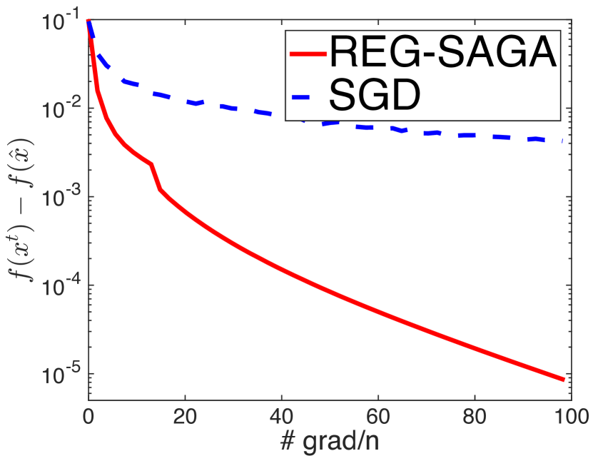
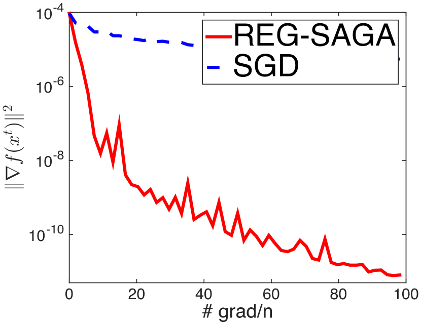
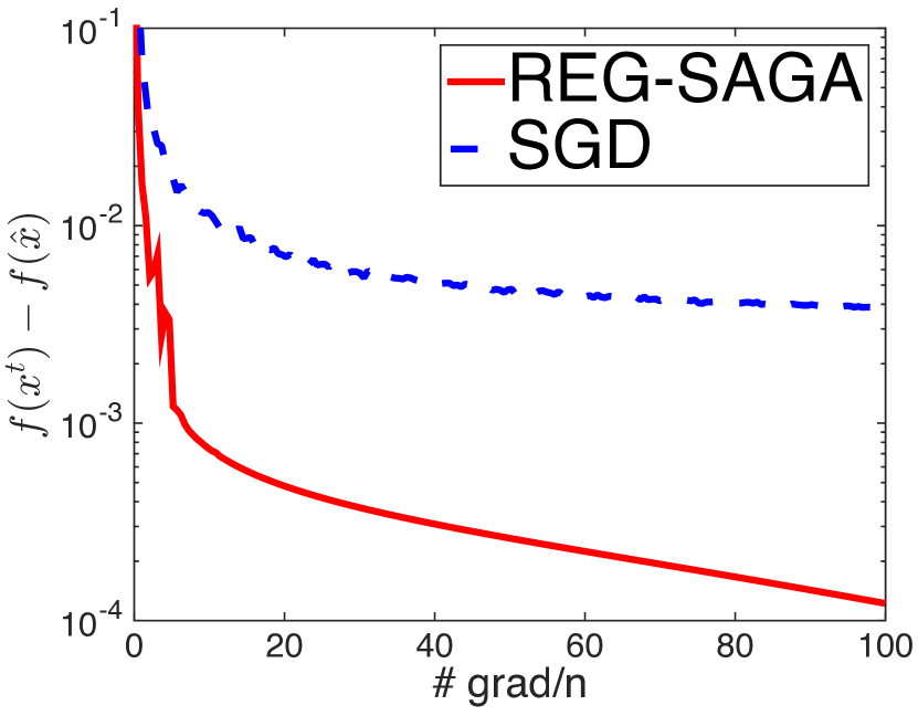
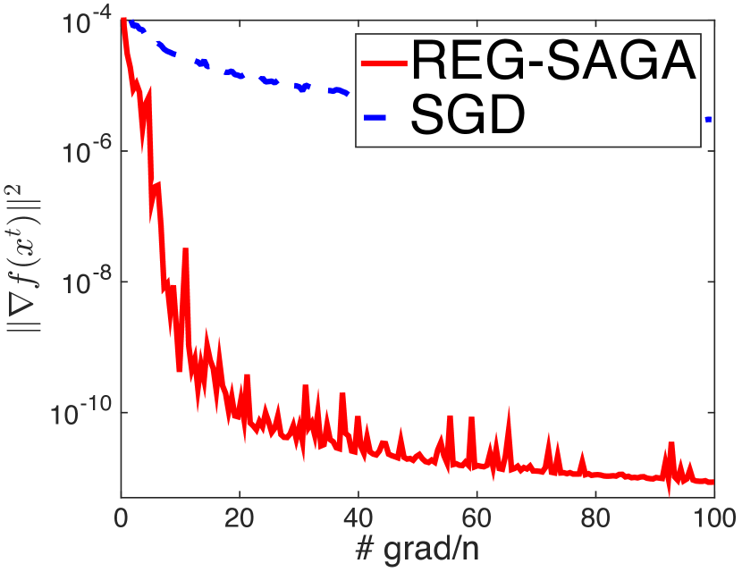
Figure 1: Results for nonconvex regularized generalized linear models (see Equation (12)). The first and last two figures correspond to rcv1 and realsim datasets respectively. The results compare the performance of Reg-Saga and Sgd algorithms. Here $\hat{x}$ corresponds to the solution obtained by running GradDescent for a very long time and using multiple restarts. As seen in the figure, Reg-Saga converges much faster than Sgd in terms of objective function value and the stationarity gap $\|\nabla f(x)\|^{2}$.

We compare the performance of Sgd (the de facto incremental method for nonconvex optimization) with nonconvex Reg-Saga in our experiments. The comparison is based on the following criteria: (i) the objective function value (also called training loss in this context), which is the main goal of the paper; and (ii) the stationarity gap $\|\nabla f(x)\|^{2}$, the criteria used for our theoretical analysis. For the step size of Sgd, we use the popular $t-$inverse schedule $\eta_{t}=\eta_{0}(1+\eta^{\prime}\lfloor t/n\rfloor)^{-1}$, where $\eta_{0}$ and $\eta^{\prime}$ are tuned so that Sgd gives the best performance on the training loss. In our experiments, we also use $\eta^{\prime}=0$; this results in a fixed step size for Sgd. For Reg-Saga, a fixed step size is chosen (as suggested by our analysis) so that it gives the best performance on the objective function value, i.e., training loss. Note that due to the structure of the problem in (12), as discussed in Section 4, the storage cost of Reg-Saga is just $O(n)$.

Initialization is critical to many of the incremental methods like Reg-Saga. This is due to the stronger dependence of the convergence on the initial point (see Theorem 3). Furthermore, one has to obtain $\nabla f_{i}(\alpha^{0}_{i})$ for all $i\in[n]$ in Reg-Saga algorithm (see Algorithm 1). For initialization of both Sgd and Reg-Saga, we make one pass (without replacement) through the dataset and perform the updates of Sgd during this pass. Doing so not only allows us to also obtain a good initial point $x^{0}$ but also to compute the initial values of $\nabla f(\alpha_{i}^{0})$ for $i\in[n]$. Note that this choice results in a variant of Reg-Saga where $\alpha_{i}^{0}$ are different for various $i$ (unlike the pseudocode in Algorithm 1). The convergence rates of this variant can be shown to be similar to that of Algorithm 1.

Figure 1 shows the results of our experiments. The results are on two standard UCI datasets, ‘rcv1’ and ‘realsim’. The plots compare the criteria mentioned earlier against the number of IFO calls made by the corresponding algorithm. For the objective function, we look at the difference between the objective function ($f(x^{t})$) and the best objective function value obtained by running GradDescent for a very large number of iterations using multiple initializations (denoted by $f(\hat{x})$). As shown in the figure, Reg-Saga converges much faster than Sgd in terms of objective value. Furthermore, as supported by the theory, the stationarity gap for Reg-Saga is very small in comparison to Sgd. Also, in our experiments, the selection of step size was much easier for Reg-Saga when compared to Sgd. Overall the empirical results for nonconvex regularized problems are promising. It will be interesting to apply the approach for other smooth nonconvex problems.

8 Conclusion

In this paper, we investigated a fast incremental method (Saga) for nonconvex optimization. Our main contribution in this paper to show that Saga can provably perform better than both Sgd and GradDescent in the context of nonconvex optimization. We also showed that with additional assumptions on function $f$ in (1) like gradient dominance, Saga has linear convergence to the global minimum as opposed to sublinear convergence of Sgd. Furthermore, for large scale parallel settings, we proposed a minibatch variant of Saga with stronger theoretical convergence rates than Sgd by attaining linear speedups in the size of the minibatches. One of the biggest advantages of Saga is the ability to use fixed step size. Such a property is important in practice since selection of step size (learning rate) for Sgd is typically difficult and is one of its biggest drawbacks.

Appendix

9 Proof of Lemma 1

Proof.

Since $f$ is $L$-smooth, from Lemma 3, we have

$$\mathbb{E}[f(x^{t+1})]\leq\mathbb{E}[f(x^{t})+\langle\nabla f(x^{t}),x^{t+1}-x^{t}\rangle$$

$$\qquad\qquad\qquad\qquad\qquad+\tfrac{L}{2}\|x^{t+1}-x^{t}\|^{2}].$$

We first note that the update in Algorithm 1 is unbiased i.e., $\mathbb{E}[v^{t}]=\nabla f(x^{t})$. By using this property of the update on the right hand side of the inequality above, we get the following:

$$\mathbb{E}[f(x^{t+1})]\leq\mathbb{E}[f(x^{t})-\eta_{t}\|\nabla f(x^{t})\|^{2}+\tfrac{L\eta^{2}}{2}\|v^{t}\|^{2}].$$ (13)

Here we used the fact that $x^{t+1}-x^{t}=-\eta v^{t}$ (see Algorithm 1). Consider now the Lyapunov function

$$R^{t}:=\mathbb{E}[f(x^{t})+\tfrac{c_{t}}{n}\sum_{i=1}^{n}\|x^{t}-\alpha_{i}^{t}\|^{2}].$$

For bounding $R^{t+1}$ we need the following:

$$\frac{1}{n}\sum_{i=1}^{n}\mathbb{E}[\|x^{t+1}-\alpha_{i}^{t+1}\|^{2}]$$

$$=\frac{1}{n}\sum_{i=1}^{n}\left[\frac{1}{n}\mathbb{E}\|x^{t+1}-x^{t}\|^{2}+\frac{n-1}{n}\underbrace{\mathbb{E}\|x^{t+1}-\alpha_{i}^{t}\|^{2}}_{T_{1}}\right].$$ (14)

The above equality from the definition of $\alpha^{t+1}_{i}$ and the uniform randomness of index $j_{t}$ in Algorithm 1. The term $T_{1}$ in (9) can be bounded as follows

$$T_{1}=\mathbb{E}[\|x^{t+1}-x^{t}+x^{t}-\alpha_{i}^{t}\|^{2}]$$

$$=\mathbb{E}[\|x^{t+1}-x^{t}\|^{2}+\|x^{t}-\alpha_{i}^{t}\|^{2}+2\langle x^{t+1}-x^{t},x^{t}-\alpha_{i}^{t}\rangle]$$

$$=\mathbb{E}[\|x^{t+1}-x^{t}\|^{2}+\|x^{t}-\alpha_{i}^{t}\|^{2}]-2\eta\mathbb{E}[\langle\nabla f(x^{t}),x^{t}-\alpha_{i}^{t}\rangle]$$

$$\leq\mathbb{E}[\|x^{t+1}-x^{t}\|^{2}+\|x^{t}-\alpha_{i}^{t}\|^{2}]$$

$$\qquad\qquad+2\eta\mathbb{E}\left[\tfrac{1}{2\beta}\|\nabla f(x^{t})\|^{2}+\tfrac{1}{2}\beta\|x^{t}-\alpha_{i}^{t}\|^{2}\right].$$ (15)

The second equality again follows from the unbiasedness of the update of Saga. The last inequality follows from a simple application of Cauchy-Schwarz and Young’s inequality. Plugging (13) and (15) into $R^{t+1}$, we obtain the following bound:

$$R^{t+1}\leq\mathbb{E}[f(x^{t})-\eta\|\nabla f(x^{t})\|^{2}+\tfrac{L\eta^{2}}{2}\|v^{t}\|^{2}]$$

$$+\mathbb{E}[c_{t+1}\|x^{t+1}-x^{t}\|^{2}+c_{t+1}\frac{n-1}{n^{2}}\sum_{i=1}^{n}\|x^{t}-\alpha_{i}^{t}\|^{2}]$$

$$+\frac{2(n-1)c_{t+1}\eta}{n^{2}}\sum_{i=1}^{n}\mathbb{E}\left[\tfrac{1}{2\beta}\|\nabla f(x^{t})\|^{2}+\tfrac{1}{2}\beta\|x^{t}-\alpha_{i}^{t}\|^{2}\right]$$

$$\leq\mathbb{E}[f(x^{t})-\left(\eta-\tfrac{c_{t+1}\eta}{\beta}\right)\|\nabla f(x^{t})\|^{2}$$

$$\qquad+\left(\tfrac{L\eta^{2}}{2}+c_{t+1}\eta^{2}\right)\mathbb{E}[\|v^{t}\|^{2}]$$

$$\qquad+\left(\frac{n-1}{n}c_{t+1}+c_{t+1}\eta\beta\right)\frac{1}{n}\sum_{i=1}^{n}\mathbb{E}\left[\|x^{t}-\alpha_{i}^{t}\|^{2}\right].$$ (16)

To further bound the quantity in (16), we use Lemma 2 to bound $\mathbb{E}[\|v^{t}\|^{2}]$, so that upon substituting it into  (16), we obtain

$$R^{t+1}\leq\mathbb{E}[f(x^{t})]$$

$$-\left(\eta-\tfrac{c_{t+1}\eta}{\beta}-\eta^{2}L-2c_{t+1}\eta^{2}\right)\mathbb{E}[\|\nabla f(x^{t})\|^{2}]$$

$$+\left[c_{t+1}\bigl{(}1-\tfrac{1}{n}+\eta\beta+2\eta^{2}L^{2}\bigr{)}+\eta^{2}L^{3}\right]\tfrac{1}{n}\sum_{i=1}^{n}\mathbb{E}\left[\|x^{t}-\alpha_{i}^{t}\|^{2}\right]$$

$$\leq R^{t}-\bigl{(}\eta-\tfrac{c_{t+1}\eta}{\beta}-\eta^{2}L-2c_{t+1}\eta^{2}\bigr{)}\mathbb{E}[\|\nabla f(x^{t})\|^{2}].$$

The second inequality follows from the definition of $c_{t}$ i.e., $c_{t}=c_{t+1}(1-\tfrac{1}{n}+\eta\beta+2\eta^{2}L^{2})+\eta^{2}L^{3}$ and $R^{t}$ specified in the statement, thus concluding the proof. ∎

10 Other Lemmas

The following lemma provides a bound on the variance of the update used in Saga algorithm. More specifically, it bounds the quantity $\mathbb{E}[\|v^{t}\|^{2}]$. A more general result for bounding the variance of the minibatch scheme in Algorithm 3 can be proved along similar lines.

Lemma 2.

Let $v^{t}$ be computed by Algorithm 1. Then,

$$\mathbb{E}[\|v^{t}\|^{2}]\leq 2\mathbb{E}[\|\nabla f(x^{t})\|^{2}]+\frac{2L^{2}}{n}\sum_{i=1}^{n}\mathbb{E}[\|x^{t}-\alpha_{i}^{t}\|^{2}].$$

Proof.

For ease of exposition, we use the notation

$$\zeta^{t}=\left(\nabla f_{i_{t}}(x^{t})-\nabla f_{i_{t}}(\alpha_{i_{t}}^{t})\right)$$

Using the convexity of $\|\!\cdot\!\|^{2}$ and the definition of $v^{t}$ we get

$$\mathbb{E}[\|v^{t}\|^{2}]=\mathbb{E}[\|\zeta^{t}+\tfrac{1}{n}\sum_{i=1}^{n}\nabla f(\alpha_{i}^{t})\|^{2}]$$

$$=\mathbb{E}[\|\zeta^{t}+\tfrac{1}{n}\sum_{i=1}^{n}\nabla f(\alpha_{i}^{t})-\nabla f(x^{t})+\nabla f(x^{t})\|^{2}]$$

$$\leq 2\mathbb{E}[\|\nabla f(x^{t})\|^{2}]+2\mathbb{E}[\|\zeta^{t}-\mathbb{E}[\zeta^{t}]\|^{2}]$$

$$\leq 2\mathbb{E}[\|\nabla f(x^{t})\|^{2}]+2\mathbb{E}[\|\zeta^{t}\|^{2}].$$

The first inequality follows from the fact that $\|a+b\|^{2}\leq 2(\|a\|^{2}+\|b\|^{2})$ and that $\mathbb{E}[\zeta^{t}]=\nabla f(x^{t})-\tfrac{1}{n}\sum_{i=1}^{n}\nabla f(\alpha_{i}^{t})$. The second inequality is obtained by noting that for a random variable $\zeta$, $\mathbb{E}[\|\zeta-\mathbb{E}[\zeta]\|^{2}]\leq\mathbb{E}[\|\zeta\|^{2}]$. Using Jensen’s inequality in the inequality above, we get

$$\mathbb{E}[\|v^{t}\|^{2}]$$

$$\leq 2\mathbb{E}[\|\nabla f(x^{t})\|^{2}]+\frac{2}{n}\sum_{i=1}^{n}\mathbb{E}[\|\nabla f_{i_{t}}(x^{t})-\nabla f_{i_{t}}(\alpha_{i}^{t})\|^{2}]$$

$$\leq 2\mathbb{E}[\|\nabla f(x^{t})\|^{2}]+\frac{2L^{2}}{n}\sum_{i=1}^{n}\mathbb{E}[\|x^{t}-\alpha_{i}^{t}\|^{2}].$$

The last inequality follows from $L$-smoothness of $f_{i_{t}}$, thus concluding the proof. ∎

The following result provides a bound on the function value of functions with Lipschitz continuous gradients.

Lemma 3.

Suppose the function $f:\mathbb{R}^{d}\rightarrow\mathbb{R}$ is $L$-smooth, then the following holds

$$f(x)\leq f(y)+\langle\nabla f(y),x-y\rangle+\frac{L}{2}\|x-y\|^{2},$$

for all $x,y\in\mathbb{R}^{d}$.

References

- Agarwal & Bottou (2014) Agarwal, Alekh and Bottou, Leon. A lower bound for the optimization of finite sums. arXiv:1410.0723, 2014.
- Agarwal & Duchi (2011) Agarwal, Alekh and Duchi, John C. Distributed delayed stochastic optimization. In Advances in Neural Information Processing Systems, pp. 873–881, 2011.
- Antoniadis et al. (2009) Antoniadis, Anestis, Gijbels, Irène, and Nikolova, Mila. Penalized likelihood regression for generalized linear models with non-quadratic penalties. Annals of the Institute of Statistical Mathematics, 63(3):585–615, June 2009.
- Bertsekas & Tsitsiklis (1989) Bertsekas, D. and Tsitsiklis, J. Parallel and Distributed Computation: Numerical Methods. Prentice-Hall, 1989.
- Bertsekas (2011) Bertsekas, Dimitri P. Incremental gradient, subgradient, and proximal methods for convex optimization: A survey. In S. Sra, S. Nowozin, S. Wright (ed.), Optimization for Machine Learning. MIT Press, 2011.
- Defazio et al. (2014) Defazio, Aaron, Bach, Francis, and Lacoste-Julien, Simon. SAGA: A fast incremental gradient method with support for non-strongly convex composite objectives. In NIPS 27, pp. 1646–1654, 2014.
- Deng & Yu (2014) Deng, Li and Yu, Dong. Deep learning: Methods and applications. Foundations and Trends Signal Processing, 7:197–387, 2014.
- Ghadimi & Lan (2013) Ghadimi, Saeed and Lan, Guanghui. Stochastic first- and zeroth-order methods for nonconvex stochastic programming. SIAM Journal on Optimization, 23(4):2341–2368, 2013. doi: 10.1137/120880811.
- Hong (2014) Hong, Mingyi. A distributed, asynchronous and incremental algorithm for nonconvex optimization: An admm based approach. arXiv preprint arXiv:1412.6058, 2014.
- James et al. (2013) James, G., Witten, D., Hastie, T., and Tibshirani, R. An Introduction to Statistical Learning: with Applications in R. Springer Texts in Statistics. Springer, 2013.
- Johnson & Zhang (2013) Johnson, Rie and Zhang, Tong. Accelerating stochastic gradient descent using predictive variance reduction. In NIPS 26, pp. 315–323, 2013.
- Kushner & Clark (2012) Kushner, Harold Joseph and Clark, Dean S. Stochastic approximation methods for constrained and unconstrained systems, volume 26. Springer Science & Business Media, 2012.
- Nemirovski et al. (2009) Nemirovski, A., Juditsky, A., Lan, G., and Shapiro, A. Robust stochastic approximation approach to stochastic programming. SIAM Journal on Optimization, 19(4):1574–1609, 2009.
- Nesterov (2003) Nesterov, Yurii. Introductory Lectures On Convex Optimization: A Basic Course. Springer, 2003.
- Nesterov & Polyak (2006) Nesterov, Yurii and Polyak, Boris T. Cubic regularization of newton method and its global performance. Mathematical Programming, 108(1):177–205, 2006.
- Polyak (1963) Polyak, B.T. Gradient methods for the minimisation of functionals. USSR Computational Mathematics and Mathematical Physics, 3(4):864–878, January 1963.
- Recht et al. (2011) Recht, Benjamin, Re, Christopher, Wright, Stephen, and Niu, Feng. Hogwild!: A Lock-Free Approach to Parallelizing Stochastic Gradient Descent. In NIPS 24, pp. 693–701, 2011.
- Reddi et al. (2015) Reddi, Sashank, Hefny, Ahmed, Sra, Suvrit, Poczos, Barnabas, and Smola, Alex J. On variance reduction in stochastic gradient descent and its asynchronous variants. In NIPS 28, pp. 2629–2637, 2015.
- Robbins & Monro (1951) Robbins, H. and Monro, S. A stochastic approximation method. Annals of Mathematical Statistics, 22:400–407, 1951.
- Schmidt et al. (2013) Schmidt, Mark W., Roux, Nicolas Le, and Bach, Francis R. Minimizing Finite Sums with the Stochastic Average Gradient. arXiv:1309.2388, 2013.
- Shalev-Shwartz (2015) Shalev-Shwartz, Shai. SDCA without duality. CoRR, abs/1502.06177, 2015.
- Shalev-Shwartz & Zhang (2013) Shalev-Shwartz, Shai and Zhang, Tong. Stochastic dual coordinate ascent methods for regularized loss. The Journal of Machine Learning Research, 14(1):567–599, 2013.
- Shamir (2014) Shamir, Ohad. A stochastic PCA and SVD algorithm with an exponential convergence rate. arXiv:1409.2848, 2014.
- Sra (2012) Sra, Suvrit. Scalable nonconvex inexact proximal splitting. In NIPS, pp. 530–538, 2012.