Scattering, bound and quasi-bound states of the generalized symmetric Woods-Saxon potential

Abstract

The exact analytical solutions of the Schrödinger equation for the generalized symmetrical Woods-Saxon potential are examined for the scattering, bound and quasi-bound states in one dimension. The reflection and transmission coefficients are analytically obtained. Then, the correlations between the potential parameters and the reflection-transmission coefficients are investigated, and a transmission resonance condition is derived. Occurrence of the transmission resonance has been shown when incident energy of the particle is equal to one of the resonance energies of the quasi-bound states.

I Introduction

The investigation of the transmission resonance of a quantum particle has raised a great deal of interest in relativistic and non-relativistic quantum mechanics in the last two decades Dombey ; Kennedy1 ; Kennedy2 ; VillalbaWSKG ; alpdogan ; nurayhulthen ; VillalbaDiracsymmetriccup ; VillalbaDiracsymmetriccup2 ; VillalbaDiracdoublebarrier ; diracmass1 ; diracmass2 , especially, the supercriticality concept which has a transmission resonance at zero momentum has been studied for scattering particles through a barrier potential that has a half bound for the inverted version of the barrier potential Dombey ; Kennedy1 ; Kennedy2 . Dombey et. al have shown that scattering of the Dirac particles through a square barrier potential lead to a transmission resonance at zero momentum. In other words their reflection and transmission coefficients are zero and one, respectively Dombey .

On the other hand, it has been shown that the Woods-Saxon potential plays an important role in atom-molecule atom and nuclear physics for both scattering and bound states Woods ; bound-scat ; scattering . In the literature, we find out that the transmission resonance and the supercriticality have been examined for a particle tunneling through Wood-Saxon potential Kennedy1 ; Kennedy2 . There, they have solved the Dirac equation in which the particle has a half-bound state for potential well at $E=-m$ and an anti-particle for the potential barrier at $E=m$. Furthermore, scattering and bound state solutions of the one-dimensional mass dependent Dirac equation with the Woods-Saxon potential have been obtained and supercriticality conditions for different mass functions have been presented diracmass1 ; diracmass2 . Not only Woods-Saxon potential, but also other potentials such as asymmetric Hulthén potential nurayhulthen , symmetric screened potential VillalbaDiracsymmetriccup ; VillalbaDiracsymmetriccup2 , a double-cusp barrier VillalbaDiracdoublebarrier have been investigated.

The transmission resonance and supercriticality concept have also been examined for a Klein-Gordon particle moving under the Woods-Saxon potential VillalbaWSKG . Rojas and Villalba have been obtained the transmission resonance for arbitrary potential parameters and have been concluded that there is no supercritical states. Moreover, solution of the Klein-Gordon equation for the asymmetric Woods-Saxon potential has been examined for both scattering and bound states. The transmission resonance and supercriticaly conditions are given in Ref. alpdogan .

In literature, not only scattering states, also bound states solutions have been studied for the Woods-Saxon potential and its modified versions for the Schrödinger EckartWS ; fluge ; bizws and the Dirac equations diracws . Furthermore, within the framework of the spin and pseudospin symmetry, the analytical solutions of the Woods-Saxon and its generalized versions are solved for Dirac equation and obtained the bound state energies with their corresponding wave functions for the particle and antiparticle pseudo1 ; nurayspin .

In this paper, we propose a potential model that is the symmetric version of the generalized Woods-Saxon potential bizws . The generalized symmetric Woods-Saxon (GSWS) potential model is more flexible and useful model than the Woods-Saxon potential in order to examine the scattering, bound and quasi-bound state solutions of the wave equations so that the GSWS potential can be applied to physical phenomena such as the scattering, transmission resonance, supercriticality, decay, fusion, fission etc.. Especially, the GSWS potential can be useful model in description of the surface interaction of the particlessurface1 ; surface2 ; surface3 ; surface4 ; surface5 . Since GSWS potential model has many applications in physics, here we show how to solve the Schrödinger equation analytically for the GSWS potential in one dimension in case of the scattering, bound and quasi-bound states. Moreover, we examine correlations between the potential parameters with the reflection-transmission coefficients in the case of scattering state, with the energy eigenvalues and their corresponding wave functions in the case of bound state, and finally with the resonance energy eigenvalues and their corresponding wave functions in the case of quasi-bound states.

In the following section, we present the analytical solution of the Schrödinger equation in one dimension for the GSWS potential model for the following cases: scattering, bound and quasi-bound states. We discuss the analytic and numeric results of the model potential. In section III, our conclusion is given.

II The Model

The GSWS potential in one dimension can be given by,

$$V(x) = \theta{(-x)}\Bigg{[}-\frac{V_{0}}{1+e^{-a(x+L)}}+\frac{W_{0}e^{-a(x+L)}}{\big{(}1+e^{-a(x+L)}\big{)}^{2}}\Bigg{]}+\theta{(x)}\Bigg{[}-\frac{V_{0}}{1+e^{a(x-L)}}+\frac{W_{0}e^{a(x-L)}}{\big{(}1+e^{a(x-L)}\big{)}^{2}}\Bigg{]},$$

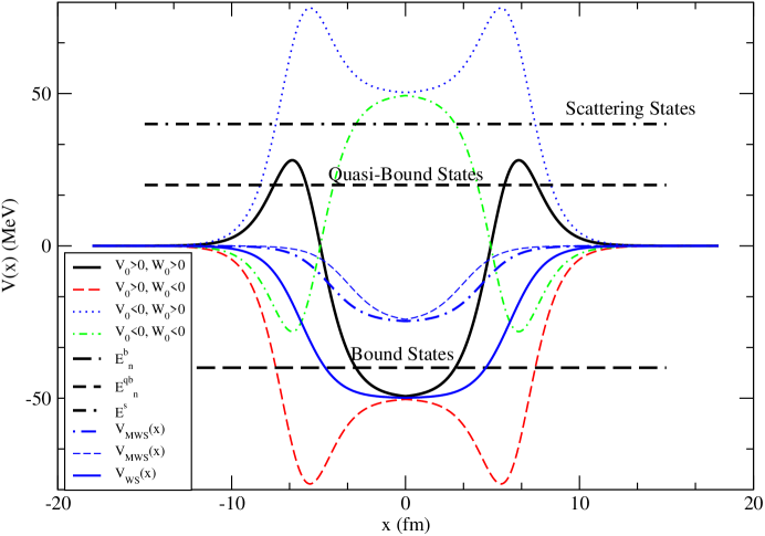
Figure 1: Shapes of the various GSWS and MWS potentials for different signs of the potential depth parameters. The magnitudes of the potential parameters are $V_{0}=50$ $MeV$, $W_{0}=200$ $MeV$, $a=1$ $fm^{-1}$ and $L=6$ $fm$. The particle energies are assumed as $E^{b}_{n}=-40$ $MeV$, $E^{qb}_{n}=20$ $MeV$ and $E^{s}=40$ $MeV$. In figure we present the bound, quasi-bound and scattering states of a particle for $V_{0}>0$ and $W_{0}>0$. The GSWS potential reduces the Woods-Saxon potential for $W=0$, $V_{WS}(x)$, (blue solid line). The blue dot-dashed line shows MWS potential $V_{MWS}(x)$ for $p=2$ and $q=10$ and the blue dashed line shows MWS potential $V_{MWS}(x)$ for $p=2$ and $q=30$.

where $\theta{(\pm x)}$ are the Heaviside step functions. The depth parameters of the potential $V_{0}$ and $W_{0}$ can be positive or negative. In the model there are other positive and real parameters $L$ and $a$, namely control parameters, adjust the shape of the potential. In Fig.(1) we present various shapes of the GSWS potential versus changing the sings of the potential depth parameters.

GSWS potential given in Eq.(II) differs from the Woods-Saxon potential by its second terms in the square brackets. While $V_{0}>0$, these terms modify the potential at the surface region which constitute either a pocket for $W_{0}<0$, or a barrier for $W_{0}>0$. This provides a great advantage in description of the interacting particle for the bound, quasi-bound and scattering states surface1 ; surface2 ; surface3 ; surface4 ; surface5 . Hence the model potential is very useful to determine the behavior of a particle in the bound, quasi-bound and scattering states. In the literature there is also the modified version of Woods-Saxon potential(MWS) similar to following equation alpdogan ,

$$V(x) = \theta{(-x)}\Bigg{[}-\frac{V_{0}}{p+qe^{-a(x+L)}}\Bigg{]}+\theta{(x)}\Bigg{[}-\frac{V_{0}}{p+qe^{a(x-L)}}\Bigg{]},$$ (2)

where $p>0$ and $q>0$ are integer numbers. In Fig.(1), we also show the WS, $V_{WS}(x)$ and MWS, $V_{MWS}(x)$ potentials. The MWS potential reduces to WS potential for $p=1$ and $q=1$ in Fig.(1). When increasing $p$ parameter, depth of the potential decreases for MWS potential. As increasing $q$, geometry of the potential changes both volume and surface regions of the potential. The GSWS potential have two advantages. Firstly, we can modify any region of the Woods-Saxon potential with surface term. The surface term of the potential has significant important in description of surface interactionsurface1 ; surface2 ; surface3 ; surface4 ; surface5 . Secondly, we can simultaneously examine interaction of the particle with GSWS potential for the bound, scattering and quasi-bound states in terms of the convenient potential parameters in Fig.(1).

In present paper we only focus on the case of $V_{0}>0$ and $W_{0}>0$ depth parameters and examine,

• the scattering states $E^{s}>0$,

• the bound states $-V_{0}<E^{b}_{n}<0$,

• the quasi-bound states $0<E^{qb}_{n}<\frac{(V_{0}-W_{0})^{2}}{4W_{0}}$.

Here $E^{b}_{n},E^{qb}_{n}$ and $E^{s}$ are the energies of the particle in the bound, quasi-bound and scattering states, respectively. The term $\frac{(V_{0}-W_{0})^{2}}{4W_{0}}$ is height of the barrier (HB) which can be derived from the potential. One can choose different signs of the potential depth parameters and examine other shapes of potential that is represented in Fig.(1) the scattering $E^{s}>0$ states in case of $V_{0}>0$ and $W_{0}<0$, one can only investigate bound and scattering states since there is no barrier term in the potential. Moreover, in case of $V_{0}<0$ and $W_{0}>0$, one can study the quasi-bound and scattering states. Finally, in case of $V_{0}<0$ $W_{0}<0$, one can examine the bound, quasi-bound and scattering states.

A final remark before we proceed, the model potential is completely symmetric with respect to y-axis i.e $V(-x)=V(x)$. Therefore we have to obtain even and odd solutions for the GSWS potential.

We consider a particle with a mass of $m$ moving under the GSWS potential, one dimensional Scrödinger equation can be given by,

$$\Big{[}\frac{d^{2}}{dx^{2}}+\frac{2m}{\hbar^{2}}\Big{(}E-V(x)\Big{)}\Big{]}\phi(x)=0.$$ (3)

Due to discontinuity in the potential, we examine the analytical solution of the GSWS potential at two regions, i.e, $x<0$ and $x>0$. Inserting Eq.(II) into Eq.(3) for $x<0$ region, we have,

$$\Bigg{[}\frac{d^{2}}{dx^{2}}+\frac{2m}{\hbar^{2}}\Bigg{(}E-\frac{W_{0}-V_{0}}{1+e^{-a(x+L)}}+\frac{W_{0}}{\big{(}1+e^{-a(x+L)}\big{)}^{2}}\Bigg{)}\Bigg{]}\phi_{L}(x) = 0.$$ (4)

By mapping $z\equiv\Big{[}1+e^{-a(x+L)}\Big{]}^{-1}$ and using the following descriptions,

$$-\epsilon^{2}\equiv\frac{2mE}{a^{2}\hbar^{2}},\,\,\ \beta^{2}\equiv\frac{2m(V_{0}-W_{0})}{a^{2}\hbar^{2}},\,\,\ \gamma^{2}\equiv\frac{2mW_{0}}{a^{2}\hbar^{2}},$$ (5)

we obtain,

$$\Bigg{[}\frac{d^{2}}{dz^{2}}+\frac{2z-1}{z(z-1)}\frac{d}{dz}+\frac{1}{z^{2}(z-1)^{2}}\bigg{(}-\epsilon^{2}+\beta^{2}z+\gamma^{2}z^{2}\bigg{)}\Bigg{]}\phi_{L}(z) = 0.$$ (6)

In this equation, there are two singular points, i.e., $z=0$ and $z=1$. In order to remove these singularities, we have to examine asymptotic behavior of Eq.(6). At $x\rightarrow-\infty$ ($z\rightarrow 0$) limit, the dominant terms in Eq.(6) are,

$$\Bigg{[}\frac{d^{2}}{dz^{2}}+\frac{1}{z}\frac{d}{dz}-\frac{\epsilon^{2}}{z^{2}}\Bigg{]}\phi_{L}(z) = 0.$$ (7)

To solve this equation we define $\phi_{L}(z)\equiv z^{\mu}$ with $\mu\equiv\epsilon\equiv\frac{ik}{a}$ and $k=\sqrt{\frac{2mE}{\hbar^{2}}}$.

On the other hand, at $x\rightarrow 0$ ($z\rightarrow 1$) limit, the dominant terms in Eq.(6) are,

$$\Bigg{[}\frac{d^{2}}{dz^{2}}+\frac{1}{z-1}\frac{d}{dz}+\frac{\beta^{2}+\gamma^{2}-\epsilon^{2}}{(z-1)^{2}}\Bigg{]}\phi_{L}(z) = 0.$$ (8)

We define $\phi_{L}(z)\equiv(z-1)^{\nu}$ with $\nu\equiv\frac{i\kappa}{a}$ and $\kappa\equiv\sqrt{\frac{2m}{\hbar^{2}}(E+V_{0})}$. Therefore we suggest the wavefunction as $\phi_{L}(z)\equiv z^{\mu}(z-1)^{\nu}f(z)$ and insert into Eq.(6) we obtain,

$$z(1-z)f{{}^{\prime\prime}}+\Big{[}(1+2\mu)-(1+2\mu+2\nu+1)z\Big{]}f^{\prime}-\Big{[}2\mu\nu+\mu+\nu+2\epsilon^{2}-\beta^{2}\Big{]}f = 0.$$ (9)

We compare Eq.(9) with the hypergeometric equation Abramowitz which is,

$$z(1-z)w{{}^{\prime\prime}}+\Big{[}c-(1+a+b)z\Big{]}w^{\prime}-abw = 0,$$ (10)

and its analytical solution is,

$$w(z) = A\,\,\,{}_{2}F_{1}[a,b,c;z]+Bz^{1-c}\,\,\,{}_{2}F_{1}[1+a-c,1+b-c,2-c;z].$$ (11)

We can easily obtain the general solution of the GSWS potential for $x<0$ region as follows:

$$\phi_{L}(z)=D_{1}z^{\mu}(z-1)^{\nu}\,\,\,{}_{2}F_{1}[a_{1},b_{1},c_{1};z]+D_{2}z^{-\mu}(z-1)^{\nu}\,\,\,{}_{2}F_{1}[1+a_{1}-c_{1},1+b_{1}-c_{1},2-c_{1};z],$$ (12)

where $a_{1}$, $b_{1}$ and $c_{1}$ are,

$$a_{1} \equiv \mu+\theta+\nu,$$

$$b_{1} \equiv 1+\mu-\theta+\nu,$$

$$c_{1} \equiv 1+2\mu.$$ (13)

Here $\theta\equiv\frac{1}{2}\mp\sqrt{\frac{1}{4}-\gamma^{2}}$.

In case of $x>0$, the one dimensional Schrödinger equation for the GSWS potential in Eq.(II) becomes,

$$\Bigg{[}\frac{d^{2}}{dx^{2}}+\frac{2m}{\hbar^{2}}\Bigg{(}E-\frac{W_{0}-V_{0}}{1+e^{a(x-L)}}+\frac{W_{0}}{\big{(}1+e^{a(x-L)}\big{)}^{2}}\Bigg{)}\Bigg{]}\phi_{R}(x) = 0.$$ (14)

By using the transformation $t\equiv\Big{[}1+e^{a(x-L)}\Big{]}^{-1}$ and the definitions in Eq.(5) we easily get,

$$\Bigg{[}\frac{d^{2}}{dt^{2}}+\frac{2t-1}{t(t-1)}\frac{d}{dt}+\frac{1}{t^{2}(t-1)^{2}}\bigg{(}-\epsilon^{2}+\beta^{2}t+\gamma^{2}t^{2}\bigg{)}\Bigg{]}\phi_{R}(t)=0.$$ (15)

By using the procedure after Eq.(6), in terms of Eq.(II) we can obtain,

$$\phi_{R}(t)=D_{3}t^{\mu}(t-1)^{\nu}\,\,\,{}_{2}F_{1}[a_{1},b_{1},c_{1};t]+D_{4}t^{-\mu}(t-1)^{\nu}\,\,\,{}_{2}F_{1}[1+a_{1}-c_{1},1+b_{1}-c_{1},2-c_{1};t].$$ (16)

After obtaining the wave function of the GSWS potential, we can examine the interaction of the particle in the GSWS potential for the case of the continuum, bound and quasi-bound states.

II.1 The Continuum States

In the continuum states, we assume that the particle is coming from negative infinity and going to positive infinity. Additionally, we could also assume the particle as incident from the right side of the potential well, due to symmetric form of the potential we could obtain the same results that we find from left side. In the continuum states the energy of the particle is positive ($E^{s}>0$ and $k>0$) and has continuum values. In all calculations, we assume $aL>>1$ which adjusts the width of the barrier. In case of continuum states the wave functions are given by Eq.(12) and Eq.(16) with $\mu=\frac{ik}{a}$ and $k=\sqrt{\frac{2mE^{s}}{\hbar^{2}}}$ for $k^{2}>0$, $\nu=\frac{i\kappa}{a}$ and $\kappa=\sqrt{\frac{2m}{\hbar^{2}}(E^{s}+V_{0})}$. In the negative domain of $x$-axis, we have to investigate the asymptotic behavior of the wave function in Eq.(12). In case of $x\rightarrow$-$\infty$ ($z\rightarrow 0$), $z\approx e^{a(x+L)}$ and ${}_{2}F_{1}[a,b,c;0]=1$. Therefore we have the incident and reflected waves,

$$\phi_{L}(x\rightarrow-\infty,z\rightarrow 0)\rightarrow e^{-\frac{\pi\kappa}{a}}\Big{(}D_{1}e^{ik(x+L)}+D_{2}e^{-ik(x+L)}\Big{)}.$$ (17)

In case of $x\rightarrow 0$ ($z\rightarrow 1$), we have to investigate the behavior of the hypergeometric function by using the relation Abramowitz ,

$${}_{2}F_{1}(a,b,c;y) = \frac{\Gamma(c)\Gamma(c-a-b)}{\Gamma(c-a)\Gamma(c-b)}\,\,\,_{2}F_{1}(a,b,a+b-c+1;1-y)$$ (18)

$$+(1-y)^{c-a-b}\frac{\Gamma(c)\Gamma(a+b-c)}{\Gamma(a)\Gamma(b)}\,\,\,_{2}F_{1}(c-a,c-b,c-a-b+1;1-y),\,\,\,\,$$

and considering $(1-z)\approx e^{-a(x+L)}$ for $z\rightarrow 1$ we get the wave function at the vicinity $z=1$ as,

$$\phi_{L}(x\rightarrow 0,z\rightarrow 1)\rightarrow\Big{[}(D_{1}N_{1}+D_{2}N_{3})e^{-i\kappa(x+L)}+(D_{1}N_{2}+D_{2}N_{4})e^{i\kappa(x+L)}\Big{]}e^{-\frac{\pi\kappa}{a}},$$ (19)

in terms of the following definitions:

$$N_{1} \equiv \frac{\Gamma(c_{1})\Gamma(c_{1}-a_{1}-b_{1})}{\Gamma(c_{1}-a_{1})\Gamma(c_{1}-b_{1})},$$

$$N_{2} \equiv \frac{\Gamma(c_{1})\Gamma(a_{1}+b_{1}-c_{1})}{\Gamma(a_{1})\Gamma(b_{1})},$$

$$N_{3} \equiv \frac{\Gamma(2-c_{1})\Gamma(c_{1}-a_{1}-b_{1})}{\Gamma(1-a_{1})\Gamma(1-b_{1})},$$

$$N_{4} \equiv \frac{\Gamma(2-c_{1})\Gamma(a_{1}+b_{1}-c_{1})}{\Gamma(1+a_{1}-c_{1})\Gamma(1+b_{1}-c_{1})}.$$ (20)

At the region $x>0$, let’s examine the behavior of the wave function in Eq.(16) for the $(x\rightarrow$$0,t\rightarrow 1)$ and $(x\rightarrow$$\infty,t\rightarrow 0)$ cases. In case of $x\rightarrow 0$ ($t\rightarrow 1$), using Eq.(18) and considering $(1-t)\approx e^{a(x-L)}$ we have,

$$\phi_{R}(x\rightarrow 0)\rightarrow\Big{[}(D_{3}M_{1}+D_{4}M_{3})e^{i\kappa(x-L)}+(D_{3}M_{2}+D_{4}M_{4})e^{-i\kappa(x-L)}\Big{]}e^{-\frac{\pi\kappa}{a}},$$ (21)

with the following relations:

$$M_{1}=N_{1},M_{2}=N_{2},M_{3}=N_{3},M_{4}=N_{4}.$$ (22)

In case of $x\rightarrow$$\infty$ ($t\rightarrow 0$), $t\approx e^{-a(x-L)}$ and ${}_{2}F_{1}[a,b,c;0]=1$. As a result we obtain the reflected and transmitted waves as follows:

$$\phi_{R}(x\rightarrow\infty,t\rightarrow 0)\rightarrow\Big{[}D_{3}e^{-ik(x-L)}(-1)^{\nu}+D_{4}e^{ik(x-L)}\Big{]}e^{-\frac{\pi\kappa}{a}}.$$ (23)

Since the potential at the infinity is not definded, the term $D_{3}$ should be zero and we have only transmitted waves for $x\rightarrow\infty$.

Since our model potential has a discontinuity due to the Heaviside step functions, we have to use the continuity conditions: At $x=0$, $\phi_{L}(x=0)=\phi_{R}(x=0)$ and $\frac{d}{dx}\phi_{L}(x=0)=\frac{d}{dx}\phi_{R}(x=0)$ should be satisfied. Therefore we get,

$$D_{1}N_{1}+D_{2}N_{3}-D_{4}M_{3} = (D_{4}M_{4}-D_{1}N_{2}-D_{2}N_{4})e^{2i\kappa L},$$ (24)

$$D_{1}N_{1}+D_{2}N_{3}+D_{4}M_{3} = (D_{4}M_{4}-D_{1}N_{2}+D_{2}N_{4})e^{2i\kappa L}.$$

Taking $N_{i}=M_{i}$ and $i=1,2,3,4$ in Eqs. (II.1) and (22) into account, and solving Eq.(24), we obtain

$$\frac{D_{2}}{D_{1}} = \frac{\Big{[}\frac{N_{1}}{N_{4}}e^{-2i\kappa L}-\frac{N_{2}}{N_{3}}e^{2i\kappa L}\Big{]}}{\Big{[}\frac{N_{4}}{N_{3}}e^{2i\kappa L}-\frac{N_{3}}{N_{4}}e^{-2i\kappa L}\Big{]}},$$ (25)

$$\frac{D_{4}}{D_{1}} = \frac{\frac{N_{1}}{N_{3}}-\frac{N_{2}}{N_{4}}}{\Big{[}\frac{N_{4}}{N_{3}}e^{2i\kappa L}-\frac{N_{3}}{N_{4}}e^{-2i\kappa L}\Big{]}}.$$ (26)

It is known that the reflected and transmitted coefficients are defined by $R=\frac{J_{refl.}}{J_{inc.}}$ and $T=\frac{J_{trans.}}{J_{inc.}}$. Here $J_{inc.}$, $J_{refl.}$ and $J_{trans.}$ are the incident, reflected and transmitted probability currents and obtained by using,

$$j(x,t) = \frac{\hbar}{2mi}\Big{[}\phi^{*}\frac{d\phi}{dx}-\phi\frac{d\phi^{*}}{dx}\Big{]},$$ (27)

which satisfies the continuity equation given by

$$\frac{\partial j(x,t)}{\partial x}+\frac{\partial\rho(x,t)}{\partial t} = 0,$$ (28)

where the probability density function $\rho(x,t)=\phi(x)^{*}\phi(x)=|\phi(x)|^{2}$. The reflection and transmission coefficients of the wave function with Eq.(27) are obtained as $R=\Big{|}\frac{D_{2}}{D_{1}}\Big{|}^{2}$ and $T=\Big{|}\frac{D_{4}}{D_{1}}\Big{|}^{2}$. Therefore we can easily get,

$$R = \frac{2-(\frac{N_{1}N_{3}}{N_{2}N_{4}}e^{-4i\kappa L}+\frac{N_{2}N_{4}}{N_{1}N_{3}}e^{4i\kappa L})}{\frac{N_{1}N_{4}}{N_{2}N_{3}}+\frac{N_{2}N_{3}}{N_{1}N_{4}}-\Big{[}\frac{N_{2}N_{4}}{N_{1}N_{3}}e^{4i\kappa L}+\frac{N_{1}N_{3}}{N_{2}N_{4}}e^{-4i\kappa L}\Big{]}},$$ (29)

and

$$T = \frac{\frac{N_{1}N_{4}}{N_{2}N_{3}}+\frac{N_{2}N_{3}}{N_{1}N_{4}}-2}{\frac{N_{1}N_{4}}{N_{2}N_{3}}+\frac{N_{2}N_{3}}{N_{1}N_{4}}-\Big{[}\frac{N_{2}N_{4}}{N_{1}N_{3}}e^{4i\kappa L}+\frac{N_{1}N_{3}}{N_{2}N_{4}}e^{-4i\kappa L}\Big{]}}.$$ (30)

In order to take into account $N_{1}^{*}=N_{4}$ and $N_{2}^{*}=N_{3}$, we can analytically obtain $R+T=1$. We would like to construct a condition for transmission resonance i.e., $T=1$ and $R=0$ Kennedy1 . In order to satisfy the resonance transmission in the transition coefficient equation, Eq.(30), the square-bracketed term in the denominator should be equal to two. Therefore we have,

$$\sin(4\kappa L)=-\frac{i}{2}\Bigg{[}\frac{(N_{1}N_{3})^{2}-(N_{2}N_{4})^{2}}{N_{1}N_{2}N_{3}N_{4}}\Bigg{]}.$$ (31)

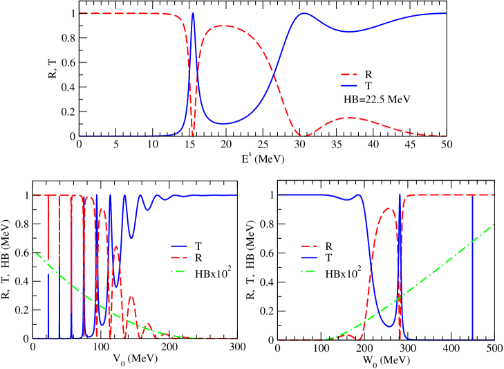
Figure 2: Variations of the reflection, transmission coefficients and the HB as a function of $E^{s}$, $V_{0}$ and $W_{0}$ parameters. Here we take $V_{0}=100$ $MeV$, $W_{0}=250$ $MeV$, $L=6$ $fm$ and $a=1$ $fm^{-1}$ for variation of R and T with $E^{s}$ on top panel. Other parameters are assumed constant, we take $E^{s}=20$ $MeV$ for variation of the $V_{0}$ and $W_{0}$ parameters. In calculations we use the following values: $mc^{2}=940$ $MeV$ and $\hbar c=197.329$ $MeV.fm$.

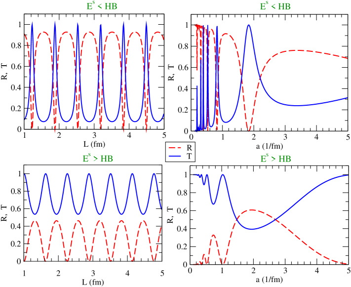
Figure 3: Variation of the reflection and transmission coefficients versus potential control parameters $a$ and $L$ in cases of $E^{s}<HB$ and $E^{s}>HB$. Here we take $V_{0}=100$ $MeV$, $W_{0}=250$ $MeV$, $mc^{2}=940$ $MeV$ and $\hbar c=197.329$ $MeV.fm$. On top panels, we present variation of $R$ and $T$ depending on $a$ and $L$ while the particle has lower energy than height of the barrier namely, $E^{s}=20$ $MeV$$<$$HB=22.5$ $MeV$ (Quantum tunneling). On bottom panels, we plot the variation of $R$ and $T$ depending on $a$ and $L$ while the particle has bigger energy than height of the barrier i.e, $E^{s}=30$ $MeV$ $>$ $HB=22.5$ $MeV$ (Resonance scattering).

It can be seen that the resonance condition depends on the potential parameters ($V_{0},W_{0},L,a$) and incident energy of the particle ($E^{s}$). In Fig.(2), the reflection and transmission coefficients are plotted as a function of incident particle energy $E^{s}$ and the depth parameters $V_{0}$ and $W_{0}$. The HB of the potential is $22.5$ $MeV$ for the parameters $V_{0}=100$ $MeV$, $W_{0}=250$ $MeV$, $L=6$ $fm$ and $a=1$ $fm^{-1}$. Therefore, as the incident energy of the particle is very low, there is a total reflection ($R=1$ and $T=0$) in Fig.(2). In calculation we cannot obtain any transmission resonance for low energy or at zero energy for any potential parameters. Increasing incident energy of the particle, the resonances begin to be observed in Fig.(2). At the resonance energy, the reflection and transmission coefficients have extremum values and their minimum and maximum values are $0$ and $1$, respectively. First resonance energy is $E^{s}=15.4913$ $MeV$ which can be obtained using Eq.(31). Other resonance energies are $30.6153$ $MeV$ and $50.37$ $MeV$. In case of $E^{s}>>HB$, increasing the incident energy of the particle, the reflection and transmission coefficients become $0$ and $1$, respectively, in Fig.(2). On the bottom of Fig.(2) we present dependencies of the reflection and transmission coefficients on depths of the potential $V_{0}$ and $W_{0}$. The HB changes with $V_{0}$ and $W_{0}$. We also plot variation of the HB with $V_{0}$ and $W_{0}$ parameters in Fig.(2)(bottom panel). In order to have the HB, it should be noted that it is $W_{0}>V_{0}$. This case is explicitly shown in Fig.(2). The maximum and minimum of the reflection and transmission coefficients depending on $V_{0}$ and $W_{0}$ parameters are apparently seen in Fig.(2). These maximum and minimum can also be calculated by using Eq.(31). For very small $V_{0}$ values the reflection and transmission coefficients are $1$ and $0$, respectively. But decreasing of height of the barrier with increasing $V_{0}$, the reflection and transmission coefficients go to $0$ and $1$, respectively, in Fig.(2) (left-bottom panel). At the minimum of the HB, the reflection and transmission coefficients are $0$ and $1$ as expected. For very small values of $W_{0}$ the reflection and transmission coefficients are $0$ and $1$ respectively since there is a very small barrier in Fig.(2) (right-bottom panel). As the HB increase with increasing $W_{0}$, the reflection and transmission coefficients go to $1$ and $0$, respectively, in Fig.(2) (right-bottom panel). In Fig.(3) we also plot variation of the reflection and transmission coefficients as a function of $a$ and $L$ parameters in case of the incident energies are lower than the HB ($E^{s}<HB$) and higher than the HB ($E^{s}>HB$). The maximum and minimum values of the reflection and transmission coefficients can be calculated by using Eq.(31) for variation of $a$ and $L$ parameters.

II.2 The Bound States

In the bound states, the particle is inside the potential well and the energy of the particle is quantized as well as $E^{b}_{n}<0$. Therefore we have $k_{n}\equiv\sqrt{-\frac{2mE^{b}_{n}}{\hbar^{2}}}$ and $\kappa_{n}\equiv\sqrt{\frac{2m}{\hbar^{2}}(E^{b}_{n}+V_{0})}$. At the $x<0$ and $x>0$ regions, the wave functions are equal to Eq.(12) and Eq.(16) respectively, with $\mu\equiv\frac{k_{n}}{a}$ and $\nu\equiv\frac{i\kappa_{n}}{a}$.

Let’s examine the asymptotic behavior of the wave function at $x<0$ region in Eq.(12) for $x\rightarrow-\infty$ ($z\rightarrow 0$). In this limit case $z\approx e^{a(x+L)}$. Therefore we have,

$$\phi_{L}(x\rightarrow-\infty,z\rightarrow 0)\rightarrow D_{1}e^{k_{n}(x+L)}(e^{i\pi\nu})+D_{2}e^{-k_{n}(x+L)}(e^{i\pi\nu}).$$ (32)

In case of bound states, the wave function should be zero for $x\rightarrow-\infty$ ($z\rightarrow 0$) in Eq.(32). Therefore second term in Eq.(32) should be zero in order to satisfy the boundary condition at $x<0$, i.e., $D_{2}=0$. As a result, the wave function at $x<0$ is

$$\phi_{L}(z)=D_{1}z^{\mu}(z-1)^{\nu}\,\,\,{}_{2}F_{1}(a,b,c;z).$$ (33)

For the case of $x\rightarrow 0$ ($z\rightarrow 1$), we have to investigate the behavior of the hypergeometric function by using the relation Eq.(18) and taking $(1-z)\approx e^{-a(x+L)}$, we get,

$$\phi_{L}(x\rightarrow 0,z\rightarrow 1)\rightarrow\Big{[}D_{1}N_{1}e^{-i\kappa_{n}(x+L)}+D_{1}N_{2}e^{i\kappa_{n}(x+L)}\Big{]}e^{-\frac{\pi\kappa_{n}}{a}},$$ (34)

where $N_{1}$ and $N_{2}$ are given in Eq.(II.1). At $x>0$ region, we have to examine asymptotic behavior of the wave function for bound states in Eq.(16). In case of $x\rightarrow 0$ ($t\rightarrow 1$), by using Eq.$(\ref{HypergeoZ=1})$ and taking $(1-t)\approx e^{a(x-L)}$ into account, we obtain,

$$\phi_{R}(x\rightarrow 0,t\rightarrow 1)\rightarrow\Big{[}(D_{3}M_{1}+D_{4}M_{3})e^{i\kappa_{n}(x-L)}+(D_{3}M_{2}+D_{4}M_{4})e^{-i\kappa_{n}(x-L)}\Big{]}e^{-\frac{\pi\kappa_{n}}{a}},$$ (35)

where $M_{1}$, $M_{2}$, $M_{3}$ and $M_{4}$ are given in Eq.(22). For the case of $x\rightarrow+\infty$ ($t\rightarrow 0$), considering $t\approx e^{-a(x-L)}$ and ${}_{2}F_{1}(a,b,c;0)=1$, we have

$$\phi_{R}(x\rightarrow\infty,t\rightarrow 0)\rightarrow\Big{[}D_{3}e^{-k_{n}(x-L)}(-1)^{\nu}+D_{4}e^{k_{n}(x-L)}\Big{]}e^{-\frac{\pi\kappa_{n}}{a}}.$$ (36)

In this equation second term does not satisfy the boundary condition i.e., $\phi_{R}(x\rightarrow\infty,t\rightarrow 0)=0$. Therefore $D_{4}$ should be zero in Eq.(36).

The left $\phi_{L}(x)$ and right $\phi_{R}(x)$ wave functions should be continuous at $x=0$. Before we apply the continuity condition, we present the latest form of the left $\phi_{L}(x)$ and right $\phi_{R}(x)$ wave functions. Taking $D_{4}=0$ in Eq. (35) and $N_{1}=M_{1}$ and $N_{2}=M_{2}$ in Eq.(22), we have

$$\phi_{L}(x\rightarrow 0)\rightarrow\Big{[}D_{1}N_{1}e^{-i\kappa_{n}(x+L)}+D_{1}N_{2}e^{i\kappa_{n}(x+L)}\Big{]}e^{-\frac{\pi\kappa_{n}}{a}},$$

$$\phi_{R}(x\rightarrow 0)\rightarrow\Big{[}D_{3}N_{1}e^{i\kappa_{n}(x-L)}+D_{3}N_{2}e^{-i\kappa_{n}(x-L)}\Big{]}e^{-\frac{\pi\kappa_{n}}{a}}.$$ (37)

By using the continuity conditions $\phi_{L}(0)=\phi_{R}(0)$, we get

$$(D_{1}-D_{3})\big{[}N_{1}e^{-i\kappa_{n}L}+N_{2}e^{i\kappa_{n}L}\big{]} = 0,$$ (38)

and using $\frac{d}{dx}\phi_{L}(x=0)=\frac{d}{dx}\phi_{R}(x=0)$ we obtain,

$$(D_{1}+D_{3})\big{[}N_{1}e^{-i\kappa_{n}L}-N_{2}e^{i\kappa_{n}L}\big{]} = 0.$$ (39)

The GSWS potential in one dimension has a symmetry under the space transformations $x\rightarrow-x$. Therefore we have even and odd solution for Eq.(38) and Eq.(39).

Even Solution: In Eq.(38), taking $D_{1}=D_{3}$ we obtain the bound state energy eigenvalue equation as,

$$E^{b}_{n} = -V_{0}+\frac{\hbar^{2}}{2mL^{2}}\Bigg{[}\arctan{\bigg{[}\frac{(N_{1}-N_{2})}{i(N_{1}+N_{2})}\bigg{]}}\pm{n\pi}\Bigg{]}^{2},n=0,1,2,...$$ (40)

and the corresponding wave function at $x<0$ as,

$$\phi_{L}(x) = D_{1}\frac{e^{\frac{k_{n}-i\kappa_{n}}{2}(x+L)-\frac{\pi\kappa_{n}}{a}}}{\big{[}2\cosh\big{(}\frac{a}{2}(x+L)\big{)}\big{]}^{\frac{k_{n}+i\kappa_{n}}{a}}}\,\,\,{}_{2}F_{1}\Big{[}a_{1},b_{1},c_{1};\frac{1}{1+e^{-a(x+L)}}\Big{]},$$ (41)

and at $x>0$ region as,

$$\phi_{R}(x) = D_{1}\frac{e^{\frac{-k_{n}+i\kappa_{n}}{2}(x-L)-\frac{\pi\kappa_{n}}{a}}}{\big{[}2\cosh\big{(}\frac{a}{2}(x-L)\big{)}\big{]}^{\frac{k_{n}+i\kappa_{n}}{a}}}\,\,\,{}_{2}F_{1}\Big{[}a_{1},b_{1},c_{1};\frac{1}{1+e^{a(x-L)}}\Big{]}.$$

Odd Solution: In Eq.(39), taking $D_{1}=-D_{3}$ we obtain the bound state energy eigenvalue equation as,

$$E^{b}_{n} = -V_{0}+\frac{\hbar^{2}}{2mL^{2}}\Bigg{[}\arctan{\bigg{[}\frac{(N_{1}+N_{2})}{i(N_{1}-N_{2})}\bigg{]}}\pm{n\pi}\Bigg{]}^{2},n=0,1,2,...$$ (43)

and the corresponding wave function at $x<0$ region as,

$$\phi_{L}(x) = D_{1}\frac{e^{\frac{k_{n}-i\kappa_{n}}{2}(x+L)-\frac{\pi\kappa_{n}}{a}}}{\big{[}2\cosh\big{(}\frac{a}{2}(x+L)\big{)}\big{]}^{\frac{k_{n}+i\kappa_{n}}{a}}}\,\,\,{}_{2}F_{1}\Big{[}a_{1},b_{1},c_{1};\frac{1}{1+e^{-a(x+L)}}\Big{]},$$ (44)

and at $x>0$ region as,

$$\phi_{R}(x) = -D_{1}\frac{e^{\frac{-k_{n}+i\kappa_{n}}{2}(x-L)-\frac{\pi\kappa_{n}}{a}}}{\big{[}2\cosh\big{(}\frac{a}{2}(x-L)\big{)}\big{]}^{\frac{k_{n}+i\kappa_{n}}{a}}}\,\,\,{}_{2}F_{1}\Big{[}a_{1},b_{1},c_{1};\frac{1}{1+e^{a(x-L)}}\Big{]}.$$ (45)

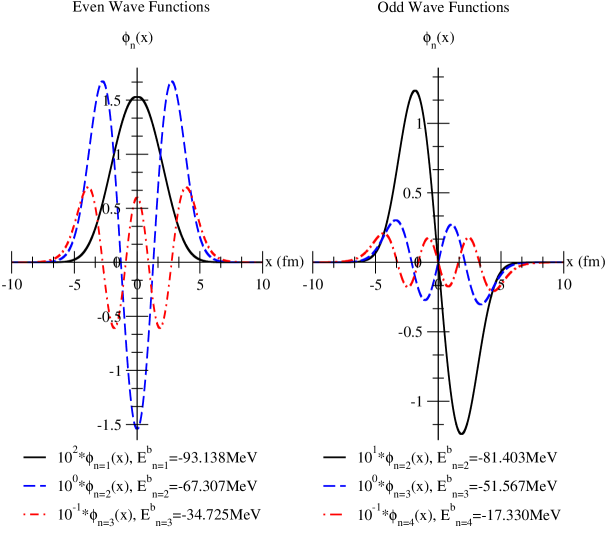
Figure 4: Plot of the even and odd unnormalized wave functions for some energy eigenvalues for the bound states. In calculations we take $V_{0}=100$ $MeV$, $W_{0}=250$ $MeV$, $L=6$ $fm$, $a=1$ $fm^{-1}$, $mc^{2}=940$ $MeV$ and $\hbar c=197.329$ $MeV.fm$.

In Fig.(4), we present the even and odd wave functions of the bound states for some energy eigenvalues by using Eqs.(40, 41) and Eq.(II.2) for even solutions as well as Eqs.(43, 44) and Eq.(45) for odd solutions. We calculate the energy eigenvalues and corresponding wave functions of the GSWS potential for the given parameters which are $V_{0}=100$ $MeV$, $W_{0}=250$ $MeV$, $L=6$ $fm$, $a=1$ $fm^{-1}$, $mc^{2}=940$ $MeV$ and $\hbar c=197.329$ $MeV.fm$. In these parameters we can only obtain four energy eigenvalues $E^{b}_{n=1}=-93.138$ $MeV$, $E^{b}_{n=2}=-67.307$ $MeV$, $E^{b}_{n=3}=-34.725$ $MeV$, $E^{b}_{n=4}=-0.125$ $MeV$ which satisfy the boundary conditions for even solutions, respectively. Similarly we show that only three energy eigenvalues can be obtained $E^{b}_{n=2}=-81.403$ $MeV$, $E^{b}_{n=3}=-51.567$ $MeV$, $E^{b}_{n=4}=-17.330$ $MeV$ which satisfy the boundary conditions for odd solutions, respectively. The number of eigenvalues depends on the parameters, namely $V_{0}$, $W_{0}$, $L$ and $a$. One can find different eigenvalues with different parameters that we choose. The higher quantum numbers $n$ do not satisfy the boundary condition of the bound states due to the positive energy. In order to obtain more solution for higher quantum numbers we have to determine boundary condition of the particle for $E^{b}_{n}>0$, namely we investigate quasi-bound state solution of the GSWS potential.

II.3 The Quasi-Bound States

In this case, the particle is inside the quantum well, but it has positive and complex energy eigenvalues, namely $E^{qb}_{n}\equiv E_{r}-iE_{i}$ and $E_{r}>>E_{i}$. By using Eq.(17) we determine the wave function for $x\rightarrow-\infty$ ($z\rightarrow 0$) as

$$\phi_{L}(x\rightarrow-\infty,z\rightarrow 0)\rightarrow D_{2}e^{-ik_{n}(x+L)}e^{-\frac{\pi\kappa_{n}}{a}},$$ (46)

where $k_{n}\equiv\sqrt{\frac{2mE^{qb}_{n}}{\hbar^{2}}}$ and $\kappa_{n}\equiv\sqrt{\frac{2m}{\hbar^{2}}(E^{qb}_{n}+V_{0})}$. In Eq.(17) we take $D_{1}=0$ since we have only outgoing wave to negative infinity. For $x\rightarrow\infty$ ($t\rightarrow 0$) we use Eq.(23) and obtain,

$$\phi_{R}(x\rightarrow\infty,t\rightarrow 0)\rightarrow D_{4}e^{ik_{n}(x-L)}e^{-\frac{\pi\kappa_{n}}{a}}.$$ (47)

In this case we have only outgoing wave that goes to positive infinity, namely $D_{3}=0$. In continuum states we already obtain the behavior of the wave functions $\phi_{L}(x)$ and $\phi_{R}(x)$ at the vicinity $x\rightarrow 0$ ($z\rightarrow 1$) and $x\rightarrow 0$ ($t\rightarrow 1$) in Eq.(19) and in Eq.(21). Considering $D_{1}=0$, $D_{3}=0$ and $N_{3}=M_{3}$ as well as $N_{4}=M_{4}$, we get,

$$\phi_{L}(x\rightarrow 0)\rightarrow\Big{[}(D_{2}N_{3})e^{-i\kappa_{n}(x+L)}+(D_{2}N_{4})e^{i\kappa_{n}(x+L)}\Big{]}e^{-\frac{\pi\kappa_{n}}{a}},$$ (48)

$$\phi_{R}(x\rightarrow 0)\rightarrow\Big{[}(D_{4}N_{3})e^{i\kappa_{n}(x-L)}+(D_{4}N_{4})e^{-i\kappa_{n}(x-L)}\Big{]}e^{-\frac{\pi\kappa_{n}}{a}}.$$ (49)

Applying the continuity conditions at $x=0$, we obtain,

$$(D_{2}-D_{4})\Big{[}N_{3}e^{-i\kappa_{n}L}+N_{4}e^{i\kappa_{n}L}\Big{]} = 0,$$ (50)

for $\phi_{L}(0)=\phi_{L}(0)$ and

$$(D_{2}+D_{4})\Big{[}N_{3}e^{-i\kappa_{n}L}-N_{4}e^{i\kappa_{n}L}\Big{]} = 0.$$ (51)

for $\frac{d}{dx}\phi_{L}(0)=\frac{d}{dx}\phi_{R}(0)$.

Even Solution: In Eq.(50), taking $D_{2}=D_{4}$ we obtain the quasi-bound state energy eigenvalue equation as,

$$E^{qb}_{n} = -V_{0}+\frac{\hbar^{2}}{2mL^{2}}\Bigg{[}\arctan{\bigg{[}\frac{(N_{3}-N_{4})}{i(N_{3}+N_{4})}\bigg{]}}\pm{n\pi}\Bigg{]}^{2},n=0,1,2,...$$ (52)

and the corresponding wave function at $x<0$ as,

$$\phi_{L}(x) = D_{2}\frac{e^{\frac{-i(\kappa_{n}+k_{n})}{2}(x+L)}e^{-\frac{\pi\kappa_{n}}{a}}}{\big{[}2\cosh\big{(}\frac{a}{2}(x+L)\big{)}\big{]}^{\frac{i(\kappa_{n}-k_{n})}{a}}}\,\,\,{}_{2}F_{1}\Big{[}1+a_{1}-c_{1},1+b_{1}-c_{1},2-c_{1};\frac{1}{1+e^{-a(x+L)}}\Big{]},\,\,\,\,\,\,\,\,\,\,\,\,$$ (53)

and at $x>0$ region as,

$$\phi_{R}(x) = D_{2}\frac{e^{\frac{-i(\kappa_{n}-k_{n})}{2}(x-L)}e^{-\frac{\pi\kappa_{n}}{a}}}{\big{[}2\cosh\big{(}\frac{a}{2}(x-L)\big{)}\big{]}^{\frac{i(\kappa_{n}+k_{n})}{a}}}\,\,\,{}_{2}F_{1}\Big{[}1+a_{1}-c_{1},1+b_{1}-c_{1},2-c_{1};\frac{1}{1+e^{a(x-L)}}\Big{]}.\,\,\,\,\,\,\,\,$$ (54)

Odd Solution: In Eq.(51), taking $D_{2}=-D_{4}$ we obtain the quasi-bound state energy eigenvalue equation as,

$$E^{qb}_{n} = -V_{0}+\frac{\hbar^{2}}{2mL^{2}}\Bigg{[}\arctan{\bigg{[}\frac{(N_{3}+N_{4})}{i(N_{3}-N_{4})}\bigg{]}}\pm{n\pi}\Bigg{]}^{2},n=0,1,2,...$$ (55)

and the corresponding wave function at $x<0$ as,

$$\phi_{L}(x) = D_{2}\frac{e^{\frac{-i(\kappa_{n}+k_{n})}{2}(x+L)}e^{-\frac{\pi\kappa_{n}}{a}}}{\big{[}2\cosh\big{(}\frac{a}{2}(x+L)\big{)}\big{]}^{\frac{i(\kappa_{n}-k_{n})}{a}}}\,\,\,{}_{2}F_{1}\Big{[}1+a_{1}-c_{1},1+b_{1}-c_{1},2-c_{1};\frac{1}{1+e^{-a(x+L)}}\Big{]},\,\,\,\,\,\,\,\,\,$$ (56)

and at $x>0$ region as,

$$\phi_{R}(x) = -D_{2}\frac{e^{\frac{-i(\kappa_{n}-k_{n})}{2}(x-L)}e^{-\frac{\pi\kappa_{n}}{a}}}{\big{[}2\cosh\big{(}\frac{a}{2}(x-L)\big{)}\big{]}^{\frac{i(\kappa_{n}+k_{n})}{a}}}\,\,\,{}_{2}F_{1}\Big{[}1+a_{1}-c_{1},1+b_{1}-c_{1},2-c_{1};\frac{1}{1+e^{a(x-L)}}\Big{]}.\,\,\,\,\,\,\,\,\,\,\,\,$$ (57)

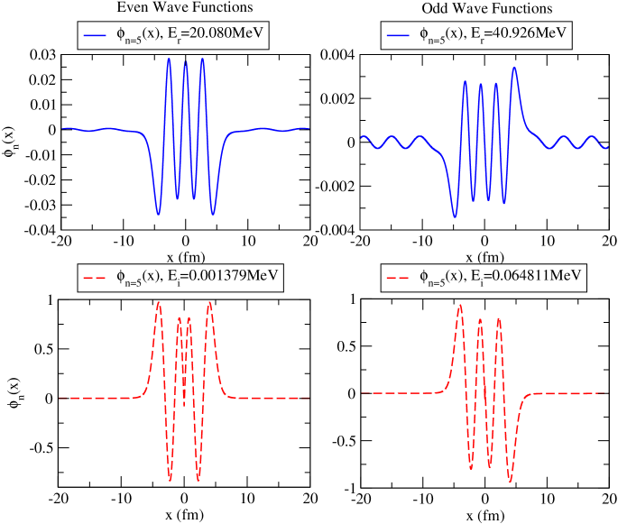
Figure 5: Plot of the even and odd unnormalized wave functions for some energy eigenvalues in case of the quasi-bound states. Here we take $V_{0}=100$ $MeV$, $W_{0}=450$ $MeV$, $L=6$ $fm$, $a=1$ $fm^{-1}$, $mc^{2}=940$ $MeV$ and $\hbar c=197.329$ $MeV.fm$.

The quasi-bound energy eigenvalues of the GSWS potential are same with bound state energy eigenvalues for E$<$0. Namely, the boundary condition of the quasi-bound state satisfies the boundary condition of bound states. By using the potential parameters in bound state calculation, we obtain the bound state energy eigenvalues and wave functions in terms of Eqs.(52, 53) and Eq.(54) for even solutions and Eqs.(55, 56) and Eq.(57) for odd solutions. In case of even solutions, for $n=5$ there are no bound and quasi-bound states since $E_{n=5}=28.6791-i4.24688$ $MeV$ and the particle energy has bigger energy value than the potential barrier ($HB=22.5$ $MeV$) and scattering occurs. In case of odd solutions, the particle has the quasi-bound energy which is $E^{qb}_{n=5}=15.431-i0.532349$ $MeV$ for $n=5$. It should be noted as the particle coming from left of the potential barrier has incident energy $E^{s}=15.431$ $MeV$, the first resonance occurs and the wave function of the particle is totally transmitted left side of the potential barrier in Fig.2. In order to obtain quasi-bound states for both even and odd solutions we increase depth of the potential barrier as $W_{0}=450$ $MeV$ by holding other terms constant. The energy eigenvalues of the quasi-bound states both even and odd solutions are $E^{qb}_{n=5}=20.0801-i0.00137933$ $MeV$ and $E^{qb}_{n=5}=40.9262-i0.0648113$ $MeV$, respectively. The resonances occur, when the energies of the particle coming from left of the potential barrier have incident energies as $E^{s}=20.0801$ $MeV$ or $E^{s}=40.9262$ $MeV$. We obtain these energies by using Eq.(31). As a result, while the energies of incident particle is equal to the quasi-bound state energy for any $n$ quantum number, the transmission resonance occurs. In Fig.(5), we show the even and odd wave functions of the particle in case of the quasi-bound states. In Fig.(5), the left and right panels show even and odd wave functions for the real and imaginary part of the energy eigenvalues of the particle.

III Conclusion

In this paper, we have presented the exact analytical solution of the Schrödinger equation for the GSWS potential. We have examined the scattering, bound and quasi-bound states of the GSWS potential and obtained the reflection and transmission coefficients in case of the scattering states, even and odd energy eigenvalues and corresponding wave functions in case of bound states as well as quasi-bound states. We have analytically shown that sum of the reflection and transmission coefficients is equal to one. We have analytically obtained the resonance condition and also investigated the correlations between the reflection-transmission coefficients and the potential parameters by considering whether the incident energy of the particle is bigger than the potential barrier or not. Then, we have analytically obtained the energy eigenvalues and corresponding even and odd wave functions for bound states. Thereafter, we have considered that the particle is inside of the potential well but has positive energy and applied the quantum boundary conditions as well as obtained the quasi-bound state energies of the particle and corresponding even-odd wave functions. We have shows that while the incident energy of the particle is equal to one of the quasi-bound state energies of the potential, there is no reflection and particle is totally transmitted from left to right side of the potential barrier. However, we could not obtain transmission resonance at low or zero incident energy of the particle for any potential parameter, namely we did not observe supercriticality for GSWS potential in non relativistic regime.

The GSWS potential model used in this paper would be useful model in order to describe scattering states of the quantum particle, which are elastic scattering, fusion etc., bound states and quasi-bound states which are the decay of quantum particle.

IV References

Dombey, N., Kennedy, P., Calogeracos, A.: Supercriticality and Transmission Resonances in the Dirac Equation. Phys. Rev. Lett. 85, 1787-1790 (2000).

Kennedy, P.: The Woods-Saxon potential in the Dirac equation. J. Phys. A: Math. Gen. 35, 689-698 (2002).

Kennedy, P. Dombey, N.: Low momentum scattering in the Dirac equation. J. Phys. A: Math. Gen. 35, 6645-6657 (2002).

Rojas, C., Villalba, V.M.: Scattering of a Klein-Gordon particle by a Woods-Saxon potential. Phys. Rev. A71, 052101 (2005).

Alpdoğan, S., Aydoğdu, O., Havare, A.: Relativistic spinless particles in the generalized asymmetric Woods-Saxon potential. J. Phys.A: Math. Theor. 46, 015301 (2013).

Candemir, N., Bayrak, O.: Massive Dirac equation in asymmetric Hulthén potential. J. Math. Phys. 54, 042104 (2013).

Villalba, V.M., Greiner, W.: Transmission resonances and supercritical states in a one-dimensional cusp potential. Phys. Rev. A67, 052707 (2003).

Villalba, V.M., González-Díaz, L.A.: Resonant states in an attractive one-dimensional cusp potential. Phys. Scr. 75, 645-650 (2007).

Villalba, V.M., González-Díaz, L.A.: Tunneling and transmission resonances of a Dirac particle by a double barrier. Phys. Scr. 81, 025010 (2010).

Panella, O., Biondini, S., Arda, A.: New exact solution of the one-dimensional Dirac equation for the Woods-Saxon potential within the effective mass case. J. Phys. A:Math. Theor. 43, 325302 (2010).

Aydoğdu, O., Arda, A., Sever, R.: Effective-mass Dirac equation for Woods-Saxon potential: Scattering, bound states, and resonances. J. Math. Phys. 53, 042106 (2012).

Costa, L.S., Prudente, F.V., Acioli, P.H., Soares Neto, J.J., Vianna, J.D.M.: A study of confined quantum systems using the Woods-Saxon potential. J. Phys. B: At. Mol. Opt. Phys. 32, 2461-2470 (1999).

Woods, R.D., Saxon, D.S.: Diffuse Surface Optical Model for Nucleon-Nuclei Scattering. Phys. Rev. 95, 577 (1954).

Brandan, M.E., Satchler, G.R.: The interaction between light heavy-ions and what it tells us. Phys. Reports 285, 143-243 (1997).

Satchler, G.R.: Heavy-ion scattering and reactions near the Coulomb barrier and ”threshold anomalies”. Phys. Reports 199, 147-190 (1991).

Zaichenko, A.K., Ol’khovskii, V.S.: Analytic solutions of the problem of scattering by potentials of the Eckart class. Theoretical and Mathematical Phys. 27, 475-477 (1976).

S. Flügge, Practical Quantum Mechanics Vol. I, Springer, Berlin, (1994).

Bayrak, O., Aciksoz, E.: Corrected analytical solution of the generalized Woods-Saxon potential for arbitrary $\ell$ states. Phys. Scr. 90, 015302 (2015).

Jian-You, G., Xiang Zheng, F., Fu-Xin, Xu.:Solution of the relativistic Dirac-Woods-Saxon problem. Phys. Rev. A66, 062105 (2002)

Guo, J.Y., Sheng, Z.Q.: Solution of the Dirac equation for the Woods-Saxon potential with spin and pseudospin symmetry. Phys. Lett. A338, 90-96 (2005).

Candemir, N., Bayrak, O.: Bound states of the Dirac equation for the generalized Woods-Saxon potential in pseudospin and spin symmetry limits. Mod. Phys. Lett. A29, 1450180 (2014).

Mackintosh, R.S., Kobos, A.M.: Evaluation of model-independent optical potentials for the O¹⁶+Ca⁴⁰ system. Phys. Rev. C26, 1766 (1982).

Boztosun, I.: New results in the analysis of ¹⁶O+²⁸Si elastic scattering by modifying the optical potential. Phys. Rev. C66, 024610 (2002).

Boztosun, I., Bayrak, O., Dagdemir, Y.: A Comparative Study of the ¹²C+²⁴Mg System with Deep and Shallow Potentials. Int. J. Mod. Phys. E14, 663-673, (2005).

Kocak, G., Karakoc, M., Boztosun, I., Balantekin, A.B.: Effects of $\alpha$-cluster potentials for the O¹⁶+O¹⁶ fusion reaction and S factor. Phys. Rev. C81, 024615 (2010).

Dapo, H., Boztosun, I., Kocak, G., Balantekin A.B.: Influence of long-range effects on low-energy cross sections of He and HeX: The lithium problem. Phys. Rev. C85, 044602 (2012).

M. Abramowitz and I.A. Stegun, Handbook of mathematical functions with formulas, graphs, and mathematical tables, Dover Publications Inc., New York.