Numerical Relativity and High Energy Physics:
Recent Developments

Abstract

We review recent progress in the application of numerical relativity techniques to astrophysics and high-energy physics. We focus on some developments that took place within the “Numerical Relativity and High Energy Physics” network, a Marie Curie IRSES action that we coordinated, namely: spin evolution in black hole binaries, high-energy black hole collisions, compact object solutions in scalar-tensor gravity, superradiant instabilities and hairy black hole solutions in Einstein’s gravity coupled to fundamental fields, and the possibility to gain insight into these phenomena using analog gravity models.

PACS numbers: 04.50.Kd, 04.70.-s, 04.70.Bw, 04.80.Cc

1 Introduction

The last global meeting of the Numerical Relativity and High Energy Physics network – a Marie Curie IRSES (International Research Staff Exchange Scheme) partnership (2012-2015) funded by the European Union and coordinated by the authors of this paper – started in Belém (Brazil) on September 28, 2015. Everyone in attendance, as well as the large majority of the scientific community, was unaware that a major breakthrough in science had just taken place: precisely two weeks earlier, the LIGO/Virgo collaboration observed the first gravitational-wave (GW) signal from the merger of two black holes (BHs) [1].

The detection relied on decades of technological efforts to perform an apparently impossible measurement, corresponding to displacements that are $\sim 10^{3}$ times smaller than the atomic nucleus. The unambiguous interpretation of the signal observed by Advanced LIGO as a BH binary coalescence was also the result of a decades-long effort: it took over 40 years to numerically solve Einstein’ equations of general relativity (GR) and to understand the behavior BH binaries through their inspiral, merger and ringdown.

A toolbox of powerful techniques became available after the tremendous numerical relativity breakthrough that took place in 2005.[2, 3, 4] This naturally led to a community effort looking for applications of these tools beyond astrophysics [5] and eventually to this network, that looked at applications of numerical relativity both in astrophysics [6] and beyond [7].

This paper is a summary of some of the science produced within the network. As such it is admittedly biased and incomplete, and it certainly does not aim to be a comprehensive review of the impressive developments in the area of numerical relativity and high-energy physics that took place over the past few years. The plan of the paper is as follows. We will start in Section 2 by considering BH collisions, first in astrophysics (paying particular attention to some recent developments concerning spin dynamics), and then in the context of fundamental and high-energy physics (with applications to large extra dimension scenarios and to the gauge gravity duality). In Section 3 we will look at compact objects – i.e., BHs and neutron stars (NSs) – in alternative theories of gravity, focusing on models with scalar degrees of freedom in the gravitational sector: tensor-(multi)-scalar theories, Horndeski gravity and Eistein-dilaton-Gauss-Bonnet gravity. In Section 4 we will consider GR minimally coupled to fundamental scalar and tensor fields and present some remarkable results obtained in the last few years in these simple models, including new types of numerical BH solutions that defied common lore. The existence of these BHs with scalar or Proca hair is intimately related with the complex phenomenon of superradiance, that can occur for rotating and charged BHs. Numerical relativity techniques have been (and will be) instrumental in probing the dynamics of these objects. Section 5 looks at many of these phenomena (in particular those discussed in Section 4) from a different perspective: that of analog gravity models. We close with some brief remarks.

2 Black hole collisions: numerical and analytical studies

Collisions of BHs have been modeled using analytic and numerical techniques for several decades. One of the main motivations throughout this time has been the significance of merging BH binary systems as one of the strongest sources for direct detection of GWs. The recent breakthrough detection by Advanced LIGO of the event called GW150914 [1] indeed observed the late stages of a BH binary inspiral, including merger and ringdown. This event clearly marks a revolution in our observational studies of the Universe. Astrophysical BH binary mergers form a key motivation for the work reviewed here. Additionally to this new era in gravitational astrophysics, many developments in theoretical physics, particularly during the past two decades, add substantial motivation to the modeling of BH collisions from other angles[7, 8], and make BHs one of the centre-stage actors in contemporary physics.

A BH is the closest analog in GR to the concept of a point mass in Newtonian physics, and spacetimes containing two BHs represent the simplest version of the two-body problem in GR. Unlike their Newtonian counterparts, however, binary BH spacetimes have substantially more complex dynamics: BHs have “internal structure” in the form of spin, and their interaction in a binary leads to GW emission. Therefore it should come as no surprise that these spacetimes cannot be described by exact solutions in closed analytic form, analogous to the Keplerian orbits in Newtonian physics. For this reason most theoretical modeling resorts to approximation methods, such as post-Newtonian theory[9], perturbation theory[10] or the point-particle approximation[11]. In alternative to these approaches, which approximate the theory, numerical relativity generates solutions to the full non-linear equations, approximating them via some form of discretization[12, 13, 14]. The decades-long efforts of numerical relativity culminated in the 2005 breakthroughs performing the first evolutions of binary BHs through inspiral, merger and ringdown [2, 3, 4]; for a historical perspective on this milestone see, e.g., Ref. Sperhake:2014wpa.

The contemporary modeling of BH collisions in the context of astrophysics, GW physics and high-energy physics relies on a combination of all these analytic and numerical methods. The purpose of this section is to review some of the most recent and exciting developments.

2.1 Astrophysical black holes and gravitational waves

The modeling of BH binaries as astrophysical sources of GWs has mostly focussed on systems in quasi-circular orbits because the emission of GWs rapidly carries away excess angular momentum from the binary [16]. By the time a binary has reached the frequency window of GW detectors such as Advanced LIGO and Advanced Virgo, the orbital eccentricity is very close to zero. This efficient elimination of eccentricity relies, of course, on the absence of any significant interaction with matter or third bodies. The possible effects of non-vanishing eccentricity have been investigated by several analytical and numerical studies [17, 18, 19, 20, 21, 22, 23, 24, 25, 26]. Quasicircular inspirals remain the most likely and best understood scenario, so here we shall concentrate on this case. We will also focus on binaries in the framework of GR, but we note that there are preliminary explorations of scalar radiation from BH binaries in scalar-tensor theory, triggered either by non asymptotically flat boundary conditions [27] or by a non-vanishing potential[28].

The estimation of source parameters in GW observations employs a method called matched filtering where the data stream is compared with a catalog of theoretically predicted GW templates [29]; for an application of this technique to hybrid waveforms constructed out of numerical relativity and PN calculations see for example Ref. Aasi:2014tra. A main challenge for the theoretical community is the generation of such template catalogs covering with high accuracy the whole range of BH binary masses and spins. Given the high computational cost of numerical relativity simulations, this construction typically stitches together post-Newtonian and numerical relativity waveforms,[31, 32, 33] or employs numerical simulations to calibrate free parameters in analytic prescriptions such as the effective-one-body model [34, 35, 36, 37].

BH binaries with generic spins will undergo spin precession during which the orbital plane changes orientation. The modeling of these systems is significantly more involved than that of their nonprecessing counterparts, but benefits enormously from the presence of three distinctly different timescales. If we denote by $r$ the separation of the two constituent BHs, these orbit around each other on the orbital timescale $t_{\rm orb}\propto r^{3/2}$, while the spin directions change on the precession timescale $t_{\rm pre}\propto r^{5/2}$, and the emission of GWs reduces the separation $r$ on the radiation reaction timescale $t_{\rm RR}\propto r^{4}$. At sufficiently large separation $r$, this implies the hierarchy $t_{\rm orb}\ll t_{\rm pre}\ll t_{\rm RR}$. The first inequality has been used to derive orbit-averaged evolution equations for the individual spin vectors $\boldsymbol{S}_{i}$ $(i=1,\,2)$ of the from $\dot{\boldsymbol{S}}_{i}=\boldsymbol{\Omega}_{i}\times\boldsymbol{S}_{i}$, where the precession frequency depends on the orbital angular momentum $\boldsymbol{L}$ and the $\boldsymbol{S}_{i}$, but not on the separation vector $\boldsymbol{r}$ [38, 39, 40]. This quasiadiabatic approach has been combined with some additional simplifications for the precession dynamics in order to construct template banks for precessing binaries. These techniques include a single effective spin model, modifications to the stationary-phase approximation, or the use of nonprecessing templates modulated through an effective precession parameter[41, 42, 43, 44, 45, 46]. Orbit-averaged PN calculations have also been employed in the discovery of spin-orbit resonances[47] and for predictions of the final spins and recoil in BH binary mergers[48, 49, 50].

The success of the orbit-averaging procedure relies heavily on the analytic solutions for Keplerian orbits that are employed in the averaging over the orbital timescale. Until recently, no analogous analytic solution was known for the precession equations, so that the second inequality of the above hierarchy, $t_{\rm orb}\ll t_{\rm RR}$, has not been brought to the same level of fruition. This picture changed with the identification of analytic solutions on the precessional timescale[51, 52]. Consider for this purpose a BH binary with orbital angular momentum $\boldsymbol{L}$, individual masses $m_{i}$ and spin vectors $\boldsymbol{S}_{i},~{}i=1,\,2$ and mass ratio $q=m_{2}/m_{1}\leq 1$. For fixed mass ratio, the system is described by nine parameters, three each for $\boldsymbol{S}_{1}$, $\boldsymbol{S}_{2}$ and $\boldsymbol{L}$. Conservation of the spin magnitudes $S_{i}$ reduces this number to seven. On the precession timescale, the total angular momentum $\boldsymbol{J}\equiv\boldsymbol{S}_{1}+\boldsymbol{S}_{2}+\boldsymbol{L}$ as well as the magnitude $L$ are also conserved at the PN orders considered here, leaving three numbers to determine the state of the binary. A convenient choice for these variables is given by the angles $\theta_{i}$ between the individual spins and the orbital angular momentum vector and the angle $\Delta\Phi$ between the projections of the individual spins onto the orbital plane: cf. e.g. Fig. 1 in Ref. Gerosa:2015tea. One further variable can be eliminated through a convenient choice of a non-inertial frame. Finally, the projected effective spin defined by[53, 54]

$$\xi\equiv(m_{1}+m_{2})^{-2}[(1+q)\boldsymbol{S}_{1}+(1+q^{-1})\boldsymbol{S}_{2}]\cdot\boldsymbol{L}/L\,,$$ (1)

is conserved by the orbit-averaged spin-precession equations at 2PN order, and even under radiation reaction at 2.5PN order. Spin precession at this order is therefore described in terms of a single evolution variable, conveniently chosen to be the magnitude of the total spin $S\equiv|\boldsymbol{S}_{1}+\boldsymbol{S}_{2}|$.

For a BH binary with specified parameters and separation, i.e. fixed values $m_{i},\,S_{i},\,L,\,J,\,\xi$, the precession is described completely in terms of the variable $S$. The set of physically allowed systems can then be represented as the area inside a closed loop constructed from two “effective potentials” $\xi_{\pm}(S)$ in the $(S,\xi)$ plane. The functions $\xi_{\pm}(S)$ are determined by the physical constraints on the spin and angular momenta

$$S_{\rm min}=\text{max}(|J-L|,\,|S_{1}-S_{2}|)\,,~{}~{}~{} S_{\rm max}=\text{min}(J+L,\,S_{1}+S_{2})\,,$$ (2)

$$J_{\rm min}=\text{max}(0,\,L-S_{1}-S_{2},\,|S_{1}-S_{2}|-L)\,,~{}~{}~{} J_{\rm max}=L+S_{1}+S_{2}\,,$$ (3)

and are given in closed analytic form by Eq. (14) in Ref. Gerosa:2015tea. For a given value of $\xi$ inside the range compatible with these constraints, this implies that $S$ oscillates between two extrema $S_{\pm}$, where $S_{\rm min}\leq S_{-}\leq S_{+}\leq S_{\rm max}$. All remaining variables of the binary can be obtained from $S$ through Eqs. (20) in Ref. Gerosa:2015tea for $\theta_{1}$, $\theta_{2}$ and $\Delta\Phi$ which, in turn, determine all other physical variables.

A particularly intriguing consequence of this formulation of the spin precession dynamics is that all binaries fall into one of three morphologies, which are best characterized by the behavior of the angle $\Delta\Phi$ on the precession time scale. As the variable $S$ oscillates inside its allowed range, $\Delta\Phi$ either (i) librates around $0$, (ii) librates around $\pi$, or (iii) circulates through the entire range $\Delta\Phi\in[-\pi,\pi]$. As the binary inspirals on the much larger radiation reaction timescale, the orbital and total angular momentum evolve, and the binary may undergo phase transitions between these morphologies. The inspiral of the binary under GW emission can be modeled in a remarkably efficient manner at 1PN order if we express the binary separation $r$ in terms of the orbital angular momentum $L$ given by the Newtonian expression $L=\eta(rM^{3})^{1/2}$, where $M\equiv m_{1}+m_{2}$ and $\eta\equiv m_{1}m_{2}/(m_{1}+m_{2})$ is the symmetric mass ratio parameter. The evolution of the total angular momentum $J$ averaged over a precession cycle is then given by[52]

$$\left\langle\frac{dJ}{dL}\right\rangle=\frac{1}{2LJ}(J^{2}-L^{2}-\langle S^{2}\rangle_{\rm pre})\,,$$ (4)

where

$$\langle S^{2}\rangle=\frac{2}{\tau}\int_{S_{-}}^{S_{+}}S^{2}\frac{dS}{|dS/dt|}\,,~{}~{}~{}~{}~{}~{}~{}~{}~{}~{}~{}~{}~{}~{}\tau\equiv 2\int_{S_{-}}^{S_{+}}\frac{dS}{|dS/dt|}\,,$$ (5)

$$\frac{dS}{dr}=-\frac{3(1-q^{2})}{2q}\,\frac{S_{1}S_{2}}{S}\,\frac{(\eta^{2}M^{3})^{3}}{L^{5}}\left(1-\frac{\eta M^{2}\xi}{L}\right)\sin\theta_{1}\,\sin\theta_{2}\,\sin\Delta\Phi\,.$$ (6)

The evolution of precessing BH binaries is thus modeled in terms of a single ordinary differential equation (4) which, thanks to the precession-averaging procedure, can furthermore be solved numerically using much larger timesteps than possible in a formulation using only orbit-averaged variables. By suitably compactifying the variables involved, accurate numerical evolutions from infinite separations become possible at drastically reduced computational cost. The formalism truly bridges the gap between astrophysical BH separations and the regime close to merger, where numerical relativity predictions for BH kicks are valid. Further applications of the formalism identified a precessional instability of binaries where the spin of the more (less) massive BH is (anti) aligned with the orbital angular momentum [55], and highlighted how the precessional morphology may carry a memory of the astrophysical processes that formed the binary[56, 52]. Preliminary studies of the potential of present and future GW detectors to determine the morphologies in BH observations are encouraging, except for highly symmetric binaries, where precessional effects are suppressed[57, 58].

2.2 Black hole collisions, fundamental and high-energy physics

Even 100 years after its publication, GR still confronts us with some of the most important questions in contemporary physics. As described below in Sec. 4, astrophysical and cosmological observations suggest the presence of an enigmatic dark sector which appears to dominate the gravitational dynamics of much of our universe. At an even more fundamental level, GR predicts the limits of its own range of validity. Seminal work by Hawking and Penrose [59, 60, 61] demonstrated that gravitational collapse in the framework of GR leads to singularities under generic initial conditions. The appearance of infinities in the theory is expected to be cured by a future quantum theory of gravitation. Quite remarkably, however, relativity appears to have a built-in protection mechanism against the potentially fatal consequences of spacetime singularities; according to Penrose’s cosmic censorship conjecture, [62] the singularities do not appear in naked form for physically realistic, generic initial data, but instead are cloaked inside horizons which causally disconnect the exterior spacetime from being influenced by the singularity. According to Thorne’s hoop conjecture, [63] such horizons should furthermore form (in $D=4$ spacetime dimensions) whenever a physical system of mass $M$ gets compacted inside a region with circumference $\lesssim 2\pi R_{s}$, where $R_{s}=2M$ is the Schwarzschild radius associated with $M$. The conjecture has also been generalized to higher dimensions[64].

A particularly intriguing consequence arising from the hoop conjecture is the possibility of BH formation in proton-proton collisions at colliders such as the LHC, or in cosmic-ray showers hitting the Earth’s atmosphere. In the trans-Planckian regime, where the colliding partons can be approximated as classical particles, the hoop conjecture predicts formation of a BH if the boost parameter $\gamma$ satisfies $\gamma\gtrsim c^{4}R/(4Gm_{0})$, i.e. if two particles of rest mass $m_{0}$ with center-of-mass energy $M=2\gamma m_{0}$ get compacted inside a volume of radius $\sim R$. Taking the radius to be given by the de Broglie wavelength $hc/M$ associated with the center-of-mass energy, the condition for BH formation becomes [65] (up to factors of order unity) $M\gtrsim E_{\rm P}=\sqrt{\hbar c^{5}/G}$, i.e. the center-of-mass energy of the collision must exceed the Planck energy. At the four-dimensional standard-model value $E_{p}\sim 10^{19}~{}{\rm GeV}$, experimental tests of BH formation are clearly out of the range of present and forseeable colliders. The so-called TeV gravity scenarios involving large or warped extra dimensions [66, 67, 68, 69], however, provide an appealing explanation of the hierarchy problem of physics and may lower the effective Planck energy to values as low as the TeV regime, which would allow for the possibility to form BHs in particle collisions at the LHC[70, 71]. Simulations of BH collisions can provide important information about the cross section and energy loss through GWs which form key input for the Monte-Carlo generators employed in the analysis of experimental data [70, 72].

Yet another rich area of applying BH studies has emerged in the context of the gauge-gravity duality, often also referred to as the AdS/CFT correspondence,[73, 74, 75] which states the equivalence between string theory in asymptotically AdS spacetimes (times a compact space) and conformal field theories living on the AdS boundary. The duality provides a new approach to the (notoriously difficult) modeling of physical systems in strongly coupled gauge theories in terms of classical spacetimes, often involving BHs, that are one dimension higher and asymptote to AdS at infinite radius.

In the following we will review some of the recent developments in BH modeling in the context of these topics, but we note that there are several more comprehensive reviews on these subjects [76, 77, 5, 7].

The hoop conjecture has been tested in the context of high-speed collisions of scalar-field [65] and fluid-ball configurations[78, 79]. In all these simulations, BH formation is observed at high velocities, consistent with the prediction of the hoop conjecture. Combined with the fact that in high-energy collisions most of the center-of-mass energy is present in the form of kinetic energy, the hoop conjecture supports the idea that parton-parton collisions can be well modeled by colliding BHs, the GR analog of point particles. High-energy collisions have been studied most comprehensively in $D=4$ spacetime dimensions and revealed a number of intriguing features. Numerical simulations of equal-mass, non-spinning BHs colliding head-on predict[80] that in the ultrarelativistic limit a fraction of $14\pm 3\%$ (recently confirmed and refined to $13\pm 1\%$ by the RIT group[81]) of the total energy is radiated in GWs. This value is about half of Penrose’s upper limit,[82, 83] and in good agreement with the value of $16.4\%$ obtained in second-order perturbative calculations on a background composed of two superposed Aichelburg-Sexl shock waves [84, 85, 86, 87, 88, 89, 90, 91, 92].

In grazing collisions the BHs are allowed to approach each other with a non-zero impact parameter $b$, and the outcome of the collision depends on whether this parameter exceeds a threshold value or not. This scattering threshold $b_{\rm scat}$ separates configurations that result in the formation of a single BH ($b<b_{\rm scat}$) or in the constituents scattering off each other to infinity ($b>b_{\rm scat}$), and was shown to be approximately given as a function of the collision speed $v$ and the center-of-mass energy $Mc^{2}$ by the remarkably simple formula  [93]

$$b_{\rm scat}\approx 2.5\frac{GM}{cv}\,.$$ (7)

Numerical simulations [94] furthermore identified the presence of zoom-whirl orbits[95] in a regime where $b$ is close to a critical value $b_{*}\lesssim b_{\rm scat}$. The energy released in GWs in these grazing collisions can be enormous, exceeding $35\%$ of the total energy. Extrapolation to the speed of light, however, demonstrates that the maximum energy saturates at about half of the total (i.e. kinetic) energy[96]. The remaining kinetic energy, instead, ends up as rest mass, either in the single BH resulting from merger or in the two constituents in scattering configurations. Simulations of rotating BHs [96] also demonstrate that the impact of the spin on the collision dynamics is washed out in the limit $v\rightarrow c$. We find here another confirmation of the “matter does not matter” conjecture already encountered in scalar-field and fluid-ball collisions[65, 78, 79]: ultrarelativistic collisions are dominated by the kinetic energy, so that the internal structure of the colliding objects becomes irrelevant for the collision process. Further evidence for this conjecture has recently been obtained in numerical studies of unequal-mass BH collisions. Head-on collisions of this type emit $\sim 13\%$ of the total mass in the form of GWs in the ultrarelativistic limit, in excellent agreement with the equal-mass result mentioned above[97].

It remains to be seen whether this picture remains intact as electric charge is added to the colliding particles. Collisions of electrically charged BHs have so far considered only the low-velocity regime, and revealed qualitatively similar dynamics as for the case of neutral BHs[98]. As intuitively expected, however, the collision is slowed down in the case of equal electric charges, reducing the energy radiated in electromagnetic and GWs as the charge-to-mass ratio approaches the critical value $Q/M=1$. Conversely, the collision is accelerated by the additional attractive force between the BHs if they carry opposite charges, which increases the GW radiation by a factor of $\sim 2.7$ as the charge-to-mass ratio $|Q|/M$ increases from 0 to 0.99  [99]. The electromagnetic radiation becomes dominant in these collisions at $|Q|/M\sim 0.37$ and exceeds its GW counterpart by a factor $\sim 5.8$ when $|Q|/M=0.99$.

The high-energy collision of particles has also attracted considerable interest in a more astrophysical context through the collisional Penrose process[100]. Particle collisions near rapidly rotating BHs could in principle lead to arbitrarily large center-of-mass energies[101], but there are several caveats on the astrophysical viability of this process[102, 103, 104]. The significance of such collisions is limited, in particular, by the redshift experienced by particles escaping from the near-horizon area to observers far away from the source[105, 106]. An interesting possibility is that one of the colliding particles could have outgoing radial momentum: this can happen either because the particle reaches a turning point in the orbit[107], or by allowing at least one outgoing particle to be generated close to the BH via previous collisions[108]. In both cases the efficiency of the process (i.e., the ratio of the escaping particle’s energy to the sum of the pre-collision particles’ energies) can reach values as large as $\sim 13.9$[109, 110].

Collisions of BHs in $D>4$ spacetime dimensions are not as well understood as the $D=4$ case, mostly because of difficulties arising in the numerical stability of the simulations. The most extensive exploration of BH collisions in $D=5$ was able to determine the scattering threshold in grazing collisions at velocities up to $v\approx 0.6~{}c$[111]. This study used the so-called modified Cartoon method[112, 113, 114, 115, 116] and identified regions of exceptionally high curvature above the Planck regime that are not hidden inside a BH horizon. These regions with curvature radius below the Planck length are realized during the close encounter of two BHs in scattering configurations. The emission of GWs in $D=5$ has been analyzed in head-on collisions of non-spinning BHs starting from rest[117, 118]. It predicts $E_{\rm rad}/M=(0.089\pm 0.006)\%$ for equal masses and a monotonic decrease, in good agreement with point particle approximations, as the mass ratio is lowered from $q=1$ to smaller values. The numerical method of this work is based on a dimensional reduction by isometry[119], analogous to the Geroch decomposition [120]. Results from the two different codes have been compared in $D=5$, demonstrating excellent agreement  [121]. This work also provided the first estimate in $D=6$, where equal-mass head-on collisions yield $E_{\rm rad}/M=(0.081\pm 0.004)\%$. All these studies assume rotational symmetry in planes involving the extra dimensions such that the effective computational domain remains three dimensional. These symmetry assumptions still accomodate most of the scenarios relevant in the context of testing TeV gravity or fundamental properties of BH spacetimes.

Perturbative calculations based on superposed shock waves have also been extended to $D\geq 5$ dimensions, including non-zero impact parameters[83, 122, 123]. These calculations predict a significant increase of the threshold impact parameter for formation of a common apparent horizon relative to the four-dimensional case; see, in particular, Table II in Ref. Yoshino:2005hi. Extension of the work by d’Eath and Payne for the head-on case to $D\geq 5$ resulted in a remarkably simple expression at first perturbative order for the energy fraction radiated in GWs [87, 88]: $E_{\rm rad}/M=1/2-1/D$. This result, originally obtained in a numerical study, has more recently been confirmed analytically to be exact at first order [91].

The modeling of shock-wave and BH collisions in asymptotically AdS spacetimes is significantly complicated by the active role and the complex structure of the outer boundary: see Refs. Bantilan:2012vu,Chesler:2013lia for a discussion of numerical methods. Over the past decade, substantial progress has been made in overcoming these difficulties, achieving the first collision of BHs in an asymptotically AdS spacetime[126] (see also Ref. Witek:2010qc for an earlier toy model). Numerical simulations of shock waves and BHs have clearly demonstrated their capacity for obtaining new insight into the strongly coupled regime of gauge theories. These studies have addressed in particular the thermalization of quark-gluon plasma in the heavy-ion collisions performed for example at the Brookhaven RHIC collider. Estimates for the thermalization time obtained through the AdS/CFT correspondence are $\sim 0.35~{}{\rm fm}/c$, in good agreement with experimental data [128, 129, 130]. As in the asymptotically flat case, point-particle and perturbative calculations provide a convenient tool complementing full numerical relativity studies [131, 132]. For a more extended discussion of BH and shock wave collisions in AdS, we refer the reader to Ref. Cardoso:2014uka.

Finally, we remark that BH collisions in asymptotically de Sitter spacetimes have been considered as tests of the cosmic censorship conjecture. The numerical simulations support the conjecture.[133]

3 Compact objects in modified theories of gravity

In this section we will discuss isolated compact objects (BHs and NSs) in modified theories of gravity. We will focus on one of the most natural and best studied extensions of GR: scalar-tensor gravity, in which one or more scalar degrees of freedom are included in the gravitational sector through a nonminimal coupling [134, 135, 136, 137, 138, 139].

We will discuss compact objects in these theories at increasing levels of complexity, starting from the “standard” Bergmann-Wagoner formulation (Section 3.1) and then considering extensions to multiple scalar fields (Section 3.2), Horndeski gravity (Section 3.3) and Einstein-dilaton-Gauss-Bonnet gravity (Section 3.4).

3.1 “Bergmann-Wagoner” scalar-tensor theories

The most general action of scalar-tensor gravity, at most quadratic in derivatives of the fields and with one scalar field, was studied by Bergmann and Wagoner [140, 141]. The action of this theory can be written (with an appropriate field redefinition) as:

$$S=\frac{1}{16\pi}\int d^{4}x\sqrt{-g}\left[\phi R-\frac{\omega(\phi)}{\phi}g^{\mu\nu}\partial_{\mu}\phi\,\partial_{\nu}\phi-U(\phi)\right]+S_{M}[\Psi,g_{\mu\nu}]\,,$$ (8)

where $U(\phi)$ and $\omega(\phi)$ are arbitrary functions of the scalar field $\phi$, and $S_{M}$ is the action of the matter fields $\Psi$. When $U(\phi)=0$ and $\omega(\phi)=\omega_{BD}$ is constant, the theory reduces to (Jordan-Fierz-)Brans-Dicke gravity [142, 143, 144].

The Bergmann-Wagoner theory (8) can be expressed in a different form through a scalar field redefinition $\varphi=\varphi(\phi)$ and a conformal transformation of the metric $g_{\mu\nu}\rightarrow g^{\star}_{\mu\nu}=A^{-2}(\varphi)g_{\mu\nu}$. In particular, fixing $A(\varphi)=\phi^{-1/2}$, the Jordan-frame action (8) transforms into the Einstein-frame action

$$S=\frac{1}{16\pi}\int d^{4}x\sqrt{-g^{\star}}\left[R^{\star}-2g^{\star\mu\nu}\partial_{\mu}\varphi\,\partial_{\nu}\varphi-V(\varphi)\right]+S_{M}[\Psi,A^{2}(\varphi)g^{\star}_{\mu\nu}]\,,$$ (9)

where $g^{\star}$ and $R^{\star}$ are the determinant and Ricci scalar of $g_{\mu\nu}^{\star}$, respectively, and the potential $V(\varphi)\equiv A^{4}(\varphi)U(\phi(\varphi))$. The price paid for the minimal coupling of the scalar field in the gravitational sector is the nontrivial coupling in the matter sector of the action: particle masses and fundamental constants depend on the scalar field.

The actions (8) and (9) are just different representations of the same theory [145, 146], so it is legitimate (and customary) to choose the conformal frame in which calculations are simpler. For instance, in vacuum the Einstein-frame action (9) formally reduces to the GR action minimally coupled with a scalar field. It may then be necessary to change the conformal frame when extracting physically meaningful statements (since the scalar field is minimally coupled to matter in the Jordan frame, test particles follow geodesics of the Jordan-frame metric, not of the Einstein-frame metric). The relation between Jordan-frame and Einstein-frame quantites is simply $\phi=A^{-2}(\varphi)$, $3+2\omega(\phi)=\alpha(\varphi)^{-2}$, where $\alpha(\varphi)\equiv d(\ln A(\varphi))/d\varphi$ [147].

Many phenomenological studies neglect the scalar potential, setting $U(\phi)=0$ or $V(\varphi)=0$. If the potential vanishes, the theory is characterized by a single function $\alpha(\varphi)$. The expansion of this function around the asymptotic value $\varphi_{0}$ can be written in the form

$$\alpha(\varphi)=\alpha_{0}+\beta_{0}(\varphi-\varphi_{0})+\dots$$ (10)

The choice $\alpha(\varphi)=\alpha_{0}=$constant (i.e., $\omega(\phi)=$constant) corresponds to Brans-Dicke theory. A more general formulation, proposed by Damour and Esposito-Farèse, is parametrized by $\alpha_{0}$ and $\beta_{0}$ [149, 150]. Another simple variant is massive Brans-Dicke theory, in which $\alpha(\varphi)$ is constant, but the potential is nonvanishing and has the form $U(\phi)=\frac{1}{2}U^{\prime\prime}(\phi_{0})(\phi-\phi_{0})^{2}$, so that the scalar field has a mass $m_{s}^{2}\sim U^{\prime\prime}(\phi_{0})$. Since the scalar field $\varphi$ in the action (9) is dimensionless, the function $\alpha(\varphi)$ and the constants $\alpha_{0}$, $\beta_{0}$ are dimensionless as well.

In the Einstein frame, the field equations are

$$G^{\star}_{\mu\nu} =2\left(\partial_{\mu}\varphi\partial_{\nu}\varphi-\frac{1}{2}g^{\star}_{\mu\nu}\partial_{\sigma}\varphi\partial^{\sigma}\varphi\right)-\frac{1}{2}g^{\star}_{\mu\nu}V(\varphi)+8\pi T^{\star}_{\mu\nu}\,,$$ (11a)

$$\Box_{g^{\star}}\varphi =-4\pi\alpha(\varphi)T^{\star}+\frac{1}{4}\frac{dV}{d\varphi}\,,$$ (11b)

where

$$T^{\star\,\mu\nu}=-\frac{2}{\sqrt{-g}}\frac{\delta S_{M}(\Psi,A^{2}g^{\star}_{\mu\nu})}{\delta g^{\star}_{\mu\nu}}$$ (12)

is the Einstein-frame stress-energy tensor of matter fields, and $T^{\star}=g^{\star\,\mu\nu}T^{\star}_{\mu\nu}$ is its trace. Eq. (11b) shows that $\alpha(\varphi)$ determines the strength of the coupling of the scalar fields to matter [134, 151].

Astrophysical observations set bounds on the parameter space of scalar-tensor theories. In the case of Brans-Dicke theory, the best observational bound ($\alpha_{0}<3.5\times 10^{-3}$) comes from the Cassini measurement of the Shapiro time delay [152]. An interesting feature of scalar-tensor gravity is the prediction of characteristic physical phenomena which do not occur in GR. Even though we know from observations that $\alpha_{0}\ll 1$ and that GR deviations are generally small, these phenomena may lead to observable consequences. The best known example is the fact that compact binary systems in scalar-tensor gravity emit dipolar gravitational radiation [153, 154]. Dipolar gravitational radiation is “pre-Newtonian,” i.e. it occurs at lower PN order than quadrupole radiation, and it does not exist in GR. In the more general case with $\beta_{0}\neq 0$, the phenomenon of spontaneous scalarization (described below) can lead in principle to macroscopic modifications in the structure of NSs, significantly affecting the amount of dipolar radiation emitted by a binary system. Therefore the best constraints in the $(\alpha_{0},\beta_{0})$ plane come from observations of NS-NS and NS-WD binary systems [155]. Observations of compact binary systems also constrain massive Brans-Dicke theory, leading to exclusion regions in the $(\alpha_{0},m_{s})$ plane [148].

3.1.1 Spontaneous scalarization in compact stars

An interesting feature of scalar-tensor theories is the existence of nonperturbative NS solutions in which the scalar field amplitude is finite even for $\alpha_{0}\ll 1$: this phenomenon, known as spontaneous scalarization [149, 150], may significantly affect the mass and radius of a NS, and therefore the orbital motion of a compact binary system, even far from coalescence. A simple way to illustrate the principle behind spontaneous scalarization is by taking the limit in which the scalar field $\varphi$ is a small perturbation around a GR solution [156]. Expanding around the constant value $\varphi_{0}$ to first order in $\hat{\varphi}\equiv\varphi-\varphi_{0}\ll 1$, the field equations in the Einstein frame (11) read

$$G_{\mu\nu}^{\star}=8\pi T_{\mu\nu}^{\star}\,,$$ (13a)

$$\square^{\star}\hat{\varphi}=-4\pi\alpha_{0}T^{\star}-4\pi\beta_{0}\hat{\varphi}T^{\star}\,.$$ (13b)

Here we have assumed analyticity around $\varphi\sim\varphi_{0}$ and we have used Eq. (10). It is clear from Eq. (13b) that $\alpha_{0}$ controls the effective coupling between the scalar and matter. Various observations, such as weak-gravity constraints and tests of violations of the strong equivalence principle, require $\alpha_{0}$ to be negligibly small when the scalar tends to its asymptotic value [157, 150, 155]. This implies that a configuration in which the scalar $\varphi\approx\varphi_{0}$ and $\alpha_{0}\approx 0$ should be at least an approximate solution in most viable scalar-tensor theories. With $\alpha_{0}=0$, any background GR solution solves the field equations above at first order in the scalar field. At this order, the Klein-Gordon equation reads

$$\left[\square^{\star}-\mu_{s}^{2}(x^{\nu})\right]\hat{\varphi}=0\,,\qquad\mu_{s}^{2}(x^{\nu})\equiv-4\pi\beta_{0}T^{\star}\,.$$ (14)

Thus, the coupling of the scalar field to matter is equivalent to an effective $x^{\nu}$-dependent mass. Depending on the sign of $\beta_{0}T^{\star}$, the effective mass squared can be negative. Because typically $-T^{\star}\approx\rho^{\star}>0$ , this happens when $\beta_{0}<0$. When $\mu_{s}^{2}<0$ in a sufficiently large region inside the NS, scalar perturbations of a GR equilibrium solution develop a tachyonic instability associated with an exponentially growing mode, which causes the growth of scalar hair in a process similar to ferromagnetism [149, 150].

Spherically symmetric NSs develop spontaneous scalarization for $\beta_{0}\lesssim-4.35$ [160]. Detailed investigations of stellar structure [150, 161], numerical simulations of collapse [162, 163, 164, 165] and stability studies [166, 160] confirmed that spontaneously scalarized configurations would indeed be the end-state of stellar collapse in these theories. This is subject, however, to the collapse process reaching a sufficient level of compactness. Recent simulations of supernova core collapse identified clear signatures of spontaneous scalarization when the collapse ultimately formed a BH, but not in case of neutron-star end products, as these were not compact enough. Further studies using more elaborate treatment of the microphysics and/or relaxing symmetry assumptions are needed to determine how generic a feature this is in core collapse scenarios. Finally, spontaneously scalarized configurations may also be the result of semiclassical vacuum instabilities [167, 168, 169, 170].

The nonradial oscillation modes of spontaneously scalarized, nonrotating stars were studied by various authors [171, 172, 173, 174]. The bottom line is that the oscillation frequencies can differ significantly from their GR counterparts if spontaneous scalarization modifies the equilibrium properties of the star (e.g., the mass-radius relation) by appreciable amounts. However, current binary pulsar observations yield very tight constraints on spontaneous scalarization – implying in particular that $\beta\gtrsim-4.5$ – and the oscillation modes of scalarized stars for viable theory parameters are unlikely to differ from their GR counterparts by any measurable amount. Note, however, that the binary pulsar constraints on $\beta$ apply to the case of massless ST theories. For massive scalars, much larger (negative) $\beta$ and correspondingly stronger effects on the structure and dynamics of compact objects may be possible [175].

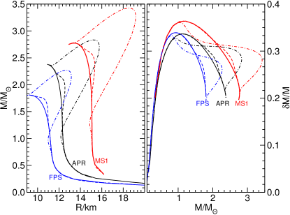
Figure 1: NS configurations in GR (solid lines) and in two scalar-tensor theories defined by Eq. (9) with $A(\varphi)\equiv e^{\frac{1}{2}\beta_{0}\varphi^{2}}$ and $V(\varphi)\equiv 0$. Dashed lines refer to $\beta_{0}=-4.5$, $\varphi_{0}^{\infty}/\sqrt{4\pi}=10^{-3}$; dash-dotted lines refer to $\beta_{0}=-6$, $\varphi_{0}^{\infty}/\sqrt{4\pi}=10^{-3}$. Each panel shows results for three different EOS models (FPS, APR and MS1). Top-left panel, left inset: relation between the nonrotating mass $M$ and the radius $R$ in the Einstein frame. Top-left panel, right inset: relative mass correction $\delta M/M$ induced by rotation at the Keplerian limit as a function of the mass $M$ of a nonspinning star with the same central energy density. Top-right panel, left inset: scalar charge $\tilde{q}/M$ as a function of $M$. Top-right panel, right inset: relative correction to the scalar charge $\delta\tilde{q}/\tilde{q}$ induced by rotation as a function of $M$. Bottom-left panel: Jordan-frame moment of inertia $\tilde{I}$ (left inset) and Jordan-frame quadrupole moment $\tilde{Q}$ (right inset) as functions of $M$. Bottom-right panel: Jordan-frame tidal ($\tilde{\lambda}$) and rotational ($\tilde{\lambda}^{\rm rot}$) Love numbers as functions of $M$. [From Pani and Berti[176].]

Spinning NSs at first order in the Hartle-Thorne slow-rotation approximation were studied by Damour and Esposito-Farèse [150] and later by Sotani [177]. At first order in rotation, the scalar field only affects the moment of inertia, mass and radius of the NS. Second-order calculations [176] are necessary to compute corrections to the spin-induced quadrupole moment, tidal and rotational Love numbers, as well as higher-order corrections to the NS mass and to the scalar charge. Figure 1 shows representative examples of the properties of NSs in a scalar-tensor theory with spontaneous scalarization at second order in the rotation parameter.

Rapidly rotating NSs in scalar-tensor theories were recently constructed [178] by extending the RNS code [179]. Scalarization effects are stronger – and deviations from GR are larger – for rapidly spinning NSs [180, 181]. Therefore, despite the tight binary pulsar bounds, it is still possible that spontaneous scalarization may occur in rapidly rotating stars.

Old, isolated NSs, as well as the NSs whose inspiral and merger we expect to observe with GW detectors, are expected to be rotating well below their mass-shedding limit. However these considerations may not apply just before merger, where the rotational frequencies of each NS may approach the mass-shedding limit. In these conditions, numerical simulations have also recently revealed the possibility of “dynamical scalarization” – a growth of the scalar field that may significantly affect the waveform near merger, and potentially be detectable [182, 183, 184, 185, 186].

A more exotic mechanism to amplify the effects of scalarization is anisotropy in the matter composing the star [187]. Nuclear matter may be anisotropic at very high densities, where the nuclear interactions must be treated relativistically and phase transitions (e.g. to pion condensates or to a superfluid state) may occur. For example, Nelmes and Piette [188] recently considered NS structure within the Skyrme model – a low energy, effective field theory for quantum chromodynamics (QCD) – finding significant anisotropic strains for stars with mass $M\gtrsim 1.5M_{\odot}$ (see also work by Adam et al.[189, 190]). The effect of anisotropy is shown in Fig. 2. For illustration, in the figure we adopt a very simple model developed in the seventies by Bowers and Liang [191], where the degree of anisotropy is parametrized by a parameter $\lambda_{\rm BL}$. The left panel shows the critical threshold for scalarization as a function of stellar compactness for several “ordinary” (isotropic) EOSs: the EOS has almost no effect on the critical threshold for scalarization, which is always around $\beta=-4.35$. The fact that scalarization is only possible when $\beta\lesssim-4.35$ was first shown by Harada[160] using catastrophe theory. In the right panel, on the other hand, we show that the critical $\beta$ for scalarization (and, as it turns out, also the effects of scalarization on macroscopic NS properties) increases (decreases) when the tangential pressure is bigger (smaller) than the radial pressure.

An interesting feature of the Bowers-Liang models is that it allows for stellar configurations with compactness approaching the Schwarzschild limit $r=2M$. Yagi and Yunes used this observation to study the recently found “I-Love-Q” universal relations – which relate bulk NS properties such as the moment of inertia, spin-induced quadrupole moment and tidal deformability in an EOS-independent way – as NSs approach the BH limit [192, 193, 194].

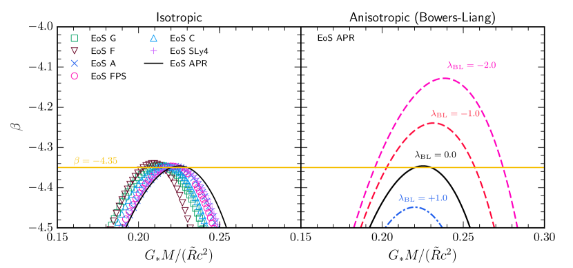
Figure 2: Effect of anisotropy on the scalarization threshold. [Adapted from Silva et al. [187].]

3.1.2 Black hole hair?

The phenomenology of scalar-tensor theory in vacuum spacetimes, such as BH spacetimes, is less interesting. When the matter action $S_{M}$ can be neglected, the Einstein-frame formulation of the theory is equivalent to GR minimally coupled to a scalar field. BHs in Bergmann-Wagoner theories satisfy the same no-hair theorem as in GR, and thus the stationary BH solutions in the two theories coincide [195, 196, 197]. Moreover, dynamical (vacuum) BH spacetimes satisfy a similar generalized no-hair theorem: the dynamics of a BH binary system in Bergmann-Wagoner theory with vanishing potential are the same as in GR [134], up to at least $2.5$ PN order for generic mass ratios [198] and at any PN order in the extreme mass-ratio limit [156].

If there is more than one massive real scalar field, however, or at least one massive complex scalar field, the situation concerning stationary BH solutions can be very different: axisymmetric, hairy BHs do exist[199, 200, 138], as will be reviewed in Section 4. Tensor-multi-scalar theories have indeed received more attention in the recent literature, as we now discuss.

3.2 Tensor-multi-scalar theories

A natural generalization of the Bergmann-Wagoner formulation (8) consists in including more than one scalar field coupled with gravity. The action of tensor-multi-scalar (TMS) gravity [134, 201] is:

$$S\,=\,\, \frac{1}{16\pi}\int d^{4}x\sqrt{-g}\left(F(\phi)R-\gamma_{ab}(\phi)g^{\mu\nu}\partial_{\mu}\phi^{a}\partial_{\nu}\phi^{b}-V(\phi)\right)+S_{M}[\Psi,\,g_{\mu\nu}]\,,$$ (15)

where $F$ and $V$ are functions of the $N$ scalar fields $\phi^{a}$ ($a=1\ldots N$). The scalar fields live on a manifold (the target space) with metric $\gamma_{ab}(\phi)$. The action (15) is invariant not only under spacetime diffeomorphisms, but also under target-space diffeomorphisms, i.e. scalar field redefinitions. TMS theories are more complex than theories with a single scalar field, since the geometry of the target space can affect the dynamics.

The simplest extension of a ST theory with a single real scalar field is a theory with two real scalar fields. If we work, equivalently, with a single complex scalar $\varphi$ instead, the action reduces to

$$S=\frac{1}{4\pi G_{\star}}\int d^{4}x\sqrt{-g}\left[\frac{R}{4}-g^{\mu\nu}\gamma(\varphi,\bar{\varphi})\nabla_{\mu}\bar{\varphi}\,\nabla_{\nu}\varphi-V(\varphi,\bar{\varphi})\right]+S_{\rm m}[A^{2}(\varphi,\bar{\varphi})g_{\mu\nu};\Psi]\,,$$

Hereafter we assume that the potential vanishes, i.e. $V(\varphi,\bar{\varphi})=0$, and that the target space is maximally symmetric. Upon stereographic projection and field redefinition[201] the target-space metric can be written as

$$\gamma(\varphi,\bar{\varphi})=\frac{1}{2}\left(1+\frac{\bar{\varphi}\varphi}{4\textswab{r}^{2}}\right)^{-2}\,,$$ (17)

where $\textswab{r}$ is the radius of curvature of the target-space geometry. For a spherical geometry we have $\textswab{r}^{2}>0$, for a hyperbolic geometry $\textswab{r}^{2}<0$, and in the limit $\textswab{r}\rightarrow\infty$ the geometry is flat.

The function $A(\varphi,\bar{\varphi})$ determines the scalar-matter coupling. What enters the field equations is actually the function $\kappa$, defined as

$$\kappa(\varphi,\bar{\varphi})\equiv 2\left(1+\frac{\bar{\varphi}\varphi}{4\mathfrak{r}^{2}}\right)\frac{\partial\log A(\varphi,\bar{\varphi})}{\partial\varphi}.$$ (18)

Without loss of generality we assume that far away from the source the field vanishes: $\varphi_{\infty}=0$. We then expand the function $\log A$ in a series about $\varphi=0$:

$$\log A(\varphi,\bar{\varphi})=\alpha^{\ast}\varphi+\bar{\alpha}^{\ast}\bar{\varphi}+\frac{1}{2}\beta_{0}\varphi\bar{\varphi}+\frac{1}{4}\beta^{\ast}_{1}\varphi^{2}+\frac{1}{4}\bar{\beta}^{\ast}_{1}\bar{\varphi}^{2}+\dots\,,$$ (19)

where $\beta_{0}$ is real, while $\alpha^{\ast}$ and $\beta^{\ast}_{1}$ are in general complex numbers. Redefine $\beta^{\ast}_{1}\equiv\beta_{1}e^{{\rm i}\theta}$, where $\theta$ is chosen such that $\beta_{1}$ is real. Then, after defining $\alpha^{\ast}\equiv\alpha e^{{\rm i}\theta/2}$ and a new field $\psi\equiv\varphi e^{{\rm i}\theta/2}$, the field equations become

$$R_{\mu\nu} =2\left(1+\frac{\bar{\psi}\psi}{4\textswab{r}^{2}}\right)^{-2}\partial_{(\mu}\bar{\psi}\partial_{\nu)}\psi+8\pi G_{\star}\left(T_{\mu\nu}-\frac{1}{2}Tg_{\mu\nu}\right)\,,$$ (20)

$$\Box\psi =\left(\frac{2\bar{\psi}}{\bar{\psi}\psi+4\textswab{r}^{2}}\right)g^{\mu\nu}\partial_{\mu}\psi\partial_{\nu}\psi-4\pi G_{\star}\left(1+\frac{\bar{\psi}\psi}{4\textswab{r}^{2}}\right)\bar{\kappa}(\psi,\bar{\psi})\,T\,,$$ (21)

where

$$\log A(\psi,\bar{\psi}) = \alpha\psi+\bar{\alpha}\bar{\psi}+\frac{1}{2}\beta_{0}\psi\bar{\psi}+\frac{1}{4}\beta_{1}\psi^{2}+\frac{1}{4}\beta_{1}\bar{\psi}^{2}+\dots\,.$$ (22)

$$= \alpha\psi+\bar{\alpha}\bar{\psi}+\frac{1}{2}\left[(\beta_{0}+\beta_{1}){\rm Re}[\psi]^{2}+(\beta_{0}-\beta_{1}){\rm Im}[\psi]^{2}\right]\,,$$

and in the second line we have split the field $\psi$ into real and imaginary parts: $\psi\equiv{\rm Re}[\psi]+{\rm i}\,{\rm Im}[\psi]$. The structure of this theory when $\alpha=0$ is determined by three real parameters: $\beta_{0}+\beta_{1}$, $\beta_{0}-\beta_{1}$ and the target-space curvature $\textswab{r}^{2}$. When $\alpha\neq 0$, two further parameters ($|\alpha|$ and $\arg\alpha$) are necessary to define the theory.

This two-scalar model is the simplest generalization of the spontaneous scalarization model by Damour and Esposito-Farèse [149]. Note that the quantity $|\alpha|^{2}\equiv\alpha\bar{\alpha}\equiv\rm{Re}[\alpha]^{2}+\rm{Im}[\alpha]^{2}$ is strongly constrained by observations, similarly to the single-scalar case. However, in TMS theories $\alpha$ is a complex quantity and its argument, $\arg\alpha$, is unconstrained in the weak-field regime. When $\alpha=0$, the conformal coupling at second order in $\psi$ reduces to

$$\log A(\psi,\bar{\psi})=\frac{1}{2}\beta_{0}\psi\bar{\psi}+\frac{1}{4}\beta_{1}\psi^{2}+\frac{1}{4}\beta_{1}\bar{\psi}^{2}\,.$$ (23)

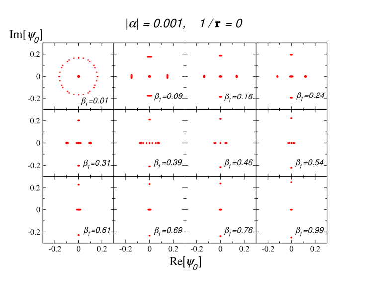
Figure 3: Scalar field amplitudes in the full TMS theory. Real and imaginary part of the scalar field amplitude at the stellar center $\psi_{0}$ for stellar models with $\beta_{0}=-5$, $|\alpha|=0.001$ and fixed baryon mass $M_{B}=1.8~{}M_{\odot}$. The different panels show the solutions found for different values of $\beta_{1}$, as indicated in each panel. In each case, we vary the phase of $\alpha$ from $0$ to $2\pi$ in steps of $\pi/6$.

Compact stars in theories with $\alpha=0$ and $\alpha\neq 0$ are rather different. When $\alpha=0$ and $\beta_{1}\neq 0$, the theory is invariant under the symmetries $\psi\to\bar{\psi}$ and $\psi\to-\psi$. In this case, we only found solutions where either the real or the imaginary part of the scalar field has a non-trivial profile; these theories are effectively equivalent to single-scalar theories.

When $\alpha\neq 0$ the situation is more interesting, as shown in Fig. 3. Introduction of $\alpha\in\mathbb{R}$ partially breaks this symmetry down to conjugation only, whereas introduction of $\alpha\in\mathbb{C}$ fully breaks the symmetry. Now GR configurations are not solutions of the field equations. In particular, a constant (or zero) scalar field does not satisfy Eq. (21) when $T\neq 0$. Therefore it is not surprising that when $\alpha\neq 0$ we can find solutions with two nontrivial scalar profiles even when $\beta_{0}=\beta_{1}=0$. A more interesting question is whether there are stellar configurations in which both scalar fields have a large amplitude. These “biscalarized” solutions are absent in the $\alpha=0$ case, but as it turns out they exist when $\alpha\neq 0$. For concreteness, in the figure we set $|\alpha|=10^{-3}$, so that the theory is compatible with experimental bounds from binary pulsar observations. We set $1/\textswab{r}=0$ (i.e., for simplicity we consider a flat target space), we fix $\beta_{0}=-5$, and we vary $\arg\alpha$ in the range $[0,\,2\pi]$ in steps of $\pi/6$. As shown in Fig. 3 – where dots denote the real and imaginary parts of the central value of the scalar field $\psi_{0}$ for which solutions were found – there are several solutions where both the real and imaginary part of the scalar field are nonzero. The solutions are at least approximately $O(2)$ symmetric when $\beta_{1}\sim|\alpha|$. The symmetry is broken (the solution “circles” turn into “crosses”) when $\beta_{1}\gg|\alpha|$, and the cross-like shape of the scalarized solutions in the $({\rm Re}[\psi_{0}]$, ${\rm Im}[\psi_{0}])$ plane collapses towards a set of solutions on the vertical line ${\rm Re}[\psi_{0}]=0$ for the larger values of $\beta_{1}$ (bottom panels in Fig. 3). For the case $\alpha=0$, it is easy to see from Eq. (22) that spontaneous scalarization of ${\rm Re}[\psi]$ occurs (in analogy with the single-field case) if $\beta_{0}+\beta_{1}\lesssim-4.35$, and that scalarized models with a large imaginary part ${\rm Im}[\psi]$ exist if $\beta_{0}-\beta_{1}\lesssim-4.35$. Our biscalarized models have been calculated for fixed $\beta_{0}=-5$. For $\beta_{1}\gtrsim 0.65$ we therefore enter the regime where $\beta_{0}+\beta_{1}\gtrsim-4.35$, and we no longer expect to find models with strongly scalarized ${\rm Re}[\psi]$. The condition $\beta_{0}-\beta_{1}\lesssim-4.35$ for scalarization of ${\rm Im}[\psi]$, however, remains satisfied, so that scalarized models should cluster close to the ${\rm Re}[\psi_{0}]$–axis. This is indeed observed in the bottom panels of Fig. 3. A more detailed investigation of the phenomenology of these models is underway.

3.3 Horndeski theories

Besides the obvious addition of one or more scalar field(s), a second possibility to generalize scalar-tensor theories of the Bergmann-Wagoner type has recently attracted a great deal of attention. The theory in question was first formulated by Horndeski [202], and it is the most general single-scalar theory with second-order field equations. In “modern” notation, the action of Horndeski gravity can be written in terms of Galileon interactions [203] as

$$S=\frac{1}{8\pi}\sum_{i=2}^{5}\int d^{4}x\sqrt{-g}{\cal L}_{i}\ ,$$ (24)

where

$${\cal L}_{2} =G_{2}\ ,$$ (25a)

$${\cal L}_{3} =-G_{3}\square\phi\ ,$$ (25b)

$${\cal L}_{4} =G_{4}R+G_{4\textnormal{X}}\left[(\square\phi)^{2}-\phi_{\mu\nu}^{2}\right]\ ,$$ (25c)

$${\cal L}_{5} =G_{5}G_{\mu\nu}\phi^{\mu\nu}-\frac{G_{5\textnormal{X}}}{6}\left[(\square\phi)^{3}+2\phi_{\mu\nu}^{3}-3\phi_{\mu\nu}^{2}\square\phi\right]\ .$$ (25d)

The functions $G_{i}=G_{i}(\phi,X)$ depend only on the scalar field $\phi$ and its kinetic energy, $X=-\partial_{\mu}\phi\partial^{\mu}\phi/2$. For brevity we have also defined the shorthand notation $\phi_{\mu\dots\nu}\equiv\nabla_{\mu}\dots\nabla_{\nu}\phi$, $\phi_{\mu\nu}^{2}\equiv\phi_{\mu\nu}\phi^{\mu\nu}$, $\phi_{\mu\nu}^{3}\equiv\phi_{\mu\nu}\phi^{\nu\alpha}\phi^{\mu}{{}_{\alpha}}$ and $\Box\phi\equiv g^{\mu\nu}\phi_{\mu\nu}$.

An attractive feature of Horndeski gravity is its generality. The theory includes a broad spectrum of phenomenological dark energy models, as well as modified gravity theories with a single scalar degree of freedom. Some important special limits of the theory are listed below:

1. GR corresponds to choosing $G_{4}=1/2$ and $G_{2}=G_{3}=G_{5}=0$.

2. When $G_{4}=F(\phi)$ and all other $G_{i}$’s are zero we recover a scalar-tensor theory with nonminimal coupling of the form $F(\phi)R$. Therefore Brans-Dicke theory and $f(R)$ gravity are special cases of Horndeski gravity.

3. A theory that we will consider in some detail below, namely Einstein-dilaton-Gauss-Bonnet (EdGB) gravity, has the action

   $$S=\frac{1}{16\pi}\int d^{4}x\sqrt{-g}\left(R+X-V(\phi)+\xi(\phi)R^{2}_{\textnormal{GB}}\right)\ ,$$ (26)

   where $V(\phi)$ is the scalar potential, $\xi(\phi)$ is a coupling function and

   $$R^{2}_{\textnormal{GB}}=R^{2}-4R_{\mu\nu}R^{\mu\nu}+R_{\alpha\beta\gamma\delta}R^{\alpha\beta\gamma\delta}$$ (27)

   is the Gauss-Bonnet invariant. This theory can be recovered with the choices[204, 205]

   $$G_{2} =\frac{X}{2}-\frac{V}{2}+4\xi^{(4)}X^{2}(3-\ln X)\,,\quad G_{3}=2\xi^{(3)}X(7-3\ln X)\,,$$ (28a)

   $$G_{4} =\frac{1}{2}+2\xi^{(2)}X(2-\ln X)\,,\quad G_{5}=-2\xi^{(1)}\ln X\,,$$ (28b)

   where we have defined $\xi^{(n)}\equiv\partial^{n}\xi/\partial\phi^{n}$ [204].

4. A theory with nonminimal derivative coupling between the scalar field $\phi$ and the Einstein tensor $G_{\mu\nu}$ (the “John” Lagrangian in the language of the so-called “Fab Four” model [206, 207]), with action

   $$S=\int d^{4}x\sqrt{-g}\left[\zeta R+2\beta X+\eta G^{\mu\nu}\phi_{\mu}\phi_{\nu}-2\Lambda_{0}\right]\,,$$ (29)

   can be constructed by setting

   $$G_{2}=-2\Lambda_{0}+2\beta X\ ,\quad G_{4}=\zeta+\eta X\ ,\quad G_{3}=G_{5}=0\ ,$$ (30)

   where $\Lambda_{0}$, $\eta$, $\zeta$ and $\beta$ are constants. Incidentally, a coupling of the form $G^{\mu\nu}\phi_{\mu}\phi_{\nu}$ can also be obtained by setting $G_{5}=-\phi$ and integrating by parts [208]

5. The Lagrangian ${\cal L}_{2}$ corresponds to the k-essence field [209, 210, 211]. For this reason, some of the literature denotes the function $G_{2}$ by the letter $K$.

6. The covariant Galileon model [212] corresponds to setting $G_{2}=-c_{2}X$, $G_{3}=-c_{3}X/M^{3}$, $G_{4}=M_{\rm Pl}^{2}/2-c_{4}X^{2}/M^{6}$ and $G_{5}=3c_{5}X^{2}/M^{9}$, where the $c_{i}$ ($i=2,\ldots,5$) are constants and $M$ is a constant with dimensions of mass.

Because of the generality of Horndeski gravity, a comprehensive review of compact objects would inevitably have to discuss important subclasses that have been studied for a long time [6]. A more specific review of compact objects in the subclasses 30–6 can be found in this same volume[213], and some examples are also discussed in another review[138]. In the next paragraph we complement these reviews focusing on recent work in EdGB gravity.

3.4 Einstein-dilaton-Gauss-Bonnet gravity

In EdGB gravity [214] (see Section 3.3), the Gauss-Bonnet invariant (27) is coupled with a scalar field  . The resulting action of EdGB gravity, Eq. (26), is a special case of Horndeski gravity, as discussed in Section 3.3. With the choice $\xi(\phi)=\alpha\phi$ this theory is shift-symmetric, and it has been shown [215] that it is the only shift-symmetric Horndeski gravity theory in which the no-hair theorems do not hold.

EdGB gravity can also be seen as belonging to a different class of modified gravity: that of quadratic gravity theories [216, 217], in which quadratic curvature terms are included in the action. EdGB gravity holds a special place as the only quadratic gravity theory with equations of motion of second differential order. Other theories of quadratic curvature gravity (e.g. dynamical Chern-Simons gravity [218, 219]) have equations of motion of higher differential order, and are then subject to Ostrogradski’s instability [220]. In order to avoid this instability they should be considered as effective theories, obtained as truncations of more general theories. In other words, EdGB gravity is consistent for any value of the coupling constant, while other quadratic gravity theories should only be considered in the weak-coupling limit. Note also that the EdGB term without the coupling to a scalar field would be trivial, since $R^{2}_{\textnormal{GB}}$ is a total derivative.

Including a quadratic curvature term in the action is an interesting modification of GR, for a variety of reasons. First of all, this is the simplest way to modify the strong-curvature regime of gravity, and, second, it is also a way to circumvent no-hair theorems (see the discussion in Sections 3.1 and 4 for different ways to grow BH hair). Moreover, quadratic curvature terms can make the theory renormalizable [221]. In particular, the EdGB term naturally arises in low-energy effective string theories [222, 223] when $\xi(\phi)=\alpha e^{\phi}/4$.

Hereafter we consider EdGB gravity with $\xi(\phi)=\alpha e^{\phi}/4$. The first BH solution of this theory, derived about 20 years ago by Kanti et al. [214], is a numerical solution describing a spherically symmetric BH. The solution has scalar hair, i.e. a non-trivial configuration of the scalar field, but only secondary hair (the scalar charge $D$ is determined by the mass $M$, and hence is not a free parameter. It can be shown that Kanti’s solution only exists for [214, 224]

$$0<\alpha/M^{2}\lesssim 0.691\,,$$ (31)

where $M$ is the BH mass. The best observational bound on the coupling parameter is $\alpha\lesssim 47\,M_{\odot}^{2}$ [225]. This bound is weaker than the theoretical bound (31) for BHs with $M\lesssim 8.2\,M_{\odot}$ [226].

In recent years, numerical solutions describing slowly rotating [224] and rapidly rotating [227] BHs have been derived. These solutions describe stationary BHs for all values of the mass and the spin, and for all values of the coupling parameter in the allowed range (31). However, these solutions require a numerical integration for each set of parameters. In order to devise and implement observational tests based on astrophysical or GW observations (for instance, for Monte Carlo data analysis), an approximate, analytical solution can be more useful than numerical solutions.

Analytical BH solutions in EdGB theory have been determined as perturbative expansions in the dimensionless coupling parameter $\zeta=\alpha/M^{2}$ and the dimensionless spin ${\bar{a}}=J/M^{2}$, at order $O(\zeta^{2},{\bar{a}}^{0})$ [228, 216], $O(\zeta^{2},{\bar{a}}^{1})$ [217], $O(\zeta^{2},{\bar{a}}^{2})$ [229], and finally at order $O(\zeta^{7},{\bar{a}}^{5})$ [230]. For a slowly rotating BH, the solution derived in [230] reproduces the most relevant geodesic quantities (the ISCO location and the epyciclic frequencies) within $1\%$, for the entire allowed range (31) of the coupling parameter.

Astrophysical observations from the near-horizon region of BHs can allow tests of GR against modified theories (such as EdGB gravity) which predict deviations in the strong-field, high-curvature regime. Indeed, near the horizon of stellar-mass BHs the spacetime curvature is very large, and (for sufficiently large values of $\alpha$) BH solutions in EdGB theory may be significantly different from the Kerr solution. These deviations can affect observable quantities, such as the quasi-periodic oscillations (QPOs) observed in the $X$-ray flux of accreting BHs [226]. Indeed, in many astrophysical models the frequencies of these QPOs are appropriate combinations of the epicyclic frequencies of the (near-horizon) BH geodesics, in which the strong-field regime of gravity is manifest. Therefore future large-area $X$-ray telescopes such as LOFT [231] could set constraints on the coupling parameter $\alpha$. For instance, the detection of two QPO triplets from a BH with $M=5.3\,M_{\odot}$ and $\bar{a}=0.2$ by a detector having the LOFT design sensitivity could exclude the range $\zeta\gtrsim 0.4$ with $3\sigma$ confidence [226].

4 Implications of superradiant instabilities for fundamental physics and astrophysics

In the previous section we focused on specific modifications of Einstein’s gravity and on the different physical consequences, as well as compact object solutions, that arise in these models. Perhaps somewhat more surprisingly, even within Einstein’s gravity, considering simple fundamental fields that satisfy the energy conditions can also lead to new types of compact objects, with interesting physical consequences. In this section we will review these recent developments, that are related to the complex phenomenon known as superradiance.[232]

4.1 Setup

Einstein’s GR minimally coupled to fundamental fields, such as massive scalars or vectors, is described by the Lagrangian

$${\cal L}=\frac{R}{\kappa}-\frac{F^{*}_{\mu\nu}F^{\mu\nu}}{4}-\frac{\mu_{V}^{2}}{2}A^{*}_{\nu}A^{\nu}-\frac{g^{\mu\nu}}{2}\phi^{\ast}_{,\mu}\phi_{,\nu}-\frac{\mu_{S}^{2}}{2}\phi^{\ast}\phi\,\ .$$ (32)

We have defined $\kappa=16\pi$, and $F_{\mu\nu}\equiv\nabla_{\mu}A_{\nu}-\nabla_{\nu}A_{\mu}$ is the Maxwell tensor. Both the scalar and vector fields are assumed to be complex, for reasons that will become clear soon. The mass $m_{B}$ of the bosons under consideration is related to the mass parameters above through $\mu_{S,V}=m_{B}/\hbar$. By “fundamental” we mean fields which are not effective descriptions of other microscopic degrees of freedom. For most of the analysis below, however, the true nature of these fields (i.e., whether they are truly fundamental or rather a coarse-grained representation of more fundamental degrees of freedom), is not relevant. Each of them is completely equivalent to two real scalar or vector fields, but some of our considerations below apply equally well to one or many real scalar and vector fields.

The theories represented by this action are relevant for several reasons. Because they are simple, they can be thought of as proxies for more complex interactions, of which they would be faithful models in certain regimes (presumably when higher-order interactions are negligible). Fundamental bosons also play a key role in particle physics. For instance they could describe the axion or axion-like particles, originally intended to solve the strong-CP problem in QCD, which recently gained prominence as dark-matter candidates [233, 234, 235]. In this context, self-gravitating solutions of fundamental fields allow us to understand and study quantitatively the growth of dark matter structures and their clustering inside compact stars [236, 237].

Whether or not they form a significant component of dark matter, minimally coupled fundamental fields should obey the equivalence principle and freely fall in the same way as standard model fields. Thus, the most promising channel to look for their imprints consists of gravitational interactions.

4.2 Superradiance and superradiant instabilities

Fundamental fields in the presence of gravity display of course a panoply of interesting effects, such as the critical phenomena identified in Choptuik’s seminal study[238]. In strong gravitational fields, one of the most peculiar is superradiance, i.e., the amplification of low-frequency waves scattering off rotating BHs [239, 240, 232]. Superradiance is required by the second law of thermodynamics, and is akin to tidal acceleration in planetary dynamics [241]. Superradiance is active for low-frequency, bosonic fields satisfying the superradiance condition

$$\omega<m\Omega\,,$$ (33)

with $m$ an integer azimuthal number and $\Omega$ the angular frequency of the BH. The amplitude of the superradiant amplification of any incident wave depends on the rotation $\Omega$, on the wave frequency $\omega$ and on the field being scattered [242, 232].

Superradiant mechanisms can trigger instabilities in spacetimes that are able to confine the fluctuations. In such cases, the wave is forced to bounce back and forth, being repeatedly amplified upon interaction with the BH, and leading to exponential growth of linearized fluctuations. This mechanism is called a black hole bomb [243, 244, 245, 246], and leads to instabilities in truly confined spacetimes like anti-de Sitter [247, 248, 249, 250, 251].

It is interesting that the same mechanism also makes Kerr BHs unstable under massive, scalar-field fluctuations [252, 253, 254, 255], vector-field fluctuations [256, 257, 258] or even tensor-field perturbations [259]. Physically, massive states prevent full leakage to infinity and act as an effective barrier for low-frequency waves.

4.3 Hairy black holes bifurcating from the Kerr solution

Since Kerr BHs are unstable against sufficiently low frequency modes of a massive bosonic field, a relevant question is: what is the endpoint of the instability? While this is still an open question (but see Section 4.3.4 below), a relevant observation is the existence of stationary, asymptotically flat BH solutions of the model (32), which are regular on and outside the event horizon and for which the horizon is in equilibrium with a non-trivial scalar or vector field condensate. Moreover these BHs are continuously connected with the Kerr solution, and as such they have been dubbed Kerr BHs with scalar [199, 260, 200] or Proca hair[261]. They are manifestly related to the phenomenon of superradiance, as they exist at the threshold of the inequality (33), and they are likely to play a role either as endpoints or as long-lived intermediate states in the development of the superradiant instability of Kerr BHs in the presence of massive scalar or vector fields.

The existence of these hairy BH solutions raises three immediate questions:

(1) “How is it possible that stationary, asymptotically flat BH solutions different from Kerr exist in the very simple model (32), in view of the well-known no-hair theorems that apply to this model (in particular the pioneering theorems due to Bekenstein for the scalar[262] and Proca[263, 264] cases)?” (see also Ref. Herdeiro:2015waa for a review of no-hair theorems applying to the scalar case).

(2) “If these hairy BH solutions are continuously connected to the Kerr solution, then there must be an imprint of their existence when we consider the corresponding matter fields on the Kerr background as test fields. Is it so?”

(3) “Do these BHs trivialize in the limit of vanishing horizon or is there some residual gravitating configuration in this limit?”

We shall tackle each of these questions in the following three subsections.

4.3.1 Circumventing no-hair theorems

The answer to ${\bf(1)}$ is simple and enlightening: theorems have assumptions and assumptions can be dropped. In the present case, an assumption in many of the no-hair theorems, including those of Bekenstein, is that the metric and the matter field share the same symmetries. This is not necessary: the spacetime and the energy-momentum tensor should share the same symmetries, but not the matter field itself. This apparently innocuous observation allows us to circumvent the simplest Bekenstein-type no-hair theorems, but observe that it is a necessary but not sufficient ingredient. The reason will become clear in the following.

The metric ansatz that has been successfully used for finding (non-extremal) Kerr BHs with scalar[199] and Proca[261] hair reads:

$$ds^{2}=-e^{2F_{0}(r,\theta)}N(r)dt^{2}+e^{2F_{1}(r,\theta)}\left[\frac{dr^{2}}{N(r)}+r^{2}d\theta^{2}\right]+r^{2}\sin^{2}\theta e^{2F_{2}(r,\theta)}[d\varphi-W(r,\theta)dt]^{2}$$ (34)

where $N(r)\equiv 1-r_{H}/r$ and $r_{H}$ is a constant. The metric is completely determined by four functions of the spheroidal coordinates $(r,\theta)$. These coordinates reduce to prolate spheroidal coordinates (rather than the more familiar oblate spheroidal ones, obtained in the flat-spacetime limit of the Boyer-Lindquist form of the Kerr metric) in an appropriate Minkowski limit.[261] A simple analysis shows that $r_{H}=$constant surfaces are null (assuming they are regular). On these surfaces, null orbits with $\theta=$ constant have an angular velocity, as measured by the observer at infinity, $\Omega_{H}\equiv W(r_{H},\theta)$. From the numerical solutions, it turns out that $\Omega_{H}$ is $\theta$-independent and $r=r_{H}$ is a Killing horizon of the Killing vector field $\xi=\partial_{t}+\Omega_{H}\partial_{\varphi}$. Thus $r=r_{H}$ is the event horizon. Observe that the line element (34) admits two independent Killing vector fields: ${\bf k}\equiv\partial_{t}$ and ${\bf m}=\partial_{\varphi}$.

On the other hand, the “matter” ansatz that has been used to find the hairy BHs is

$$\Psi(t,r,\theta,\varphi)=e^{-i\omega t+im\varphi}\phi(r,\theta)$$ (35)

for the scalar case[199], and

$$A(t,r,\theta,\varphi)=e^{-i\omega t+im\varphi}\{i[V(r,\theta)dt+H_{3}(r,\theta)\sin\theta d\varphi]+H_{1}(r,\theta)dr+H_{2}(r,\theta)d\theta\}\ ,$$ (36)

for the Proca case.[261] The two constant parameters $\omega,m$ are the frequency and azimuthal quantum number, with $\omega\in\mathbb{R^{+}}$, $m\in\mathbb{Z}/\{0\}$. An immediate observation is that the matter fields are not invariant under the two aforementioned Killing vector fields:

$$\mathcal{L}_{\bf k}A_{\mu}\neq 0\ ,\qquad\mathcal{L}_{\bf m}A_{\mu}\neq 0\ ,\qquad\mathcal{L}_{\bf k}\Psi\neq 0\ ,\qquad\mathcal{L}_{\bf m}\Psi\neq 0\ ,$$ (37)

but the corresponding energy momentum-tensors are

$$\mathcal{L}_{\bf k}T^{(\Psi)}_{\alpha\beta}=0\ ,\qquad\mathcal{L}_{\bf k}T^{(A)}_{\alpha\beta}=0\ ,\qquad\mathcal{L}_{\bf m}T^{(\Psi)}_{\alpha\beta}=0\ ,\qquad\mathcal{L}_{\bf m}T^{(A)}_{\alpha\beta}=0\ .$$ (38)

Thus Bekenstein-type theorems are inapplicable and the absence of hair is no longer guaranteed, but the left- and right-hand sides of the Einstein equations still have the same symmetries.

The ansatz (34), in combination with (35) or (36), yields axially symmetric solutions. One may wonder whether BH solutions could also exist in the much simpler spherically symmetric case, obtained by taking $W=0$ and $F_{1}=F_{2}$ in (34) and $m=0$ and $\phi=\phi(r)$ in (35); $H_{2}=H_{3}=0$ and $V=V(r)$, $H_{1}=H_{1}(r)$ in (36), respectively. In that case, however, it was shown for both the scalar case[265] and the Proca case[261] that no BH solutions exist. Thus, as mentioned above, symmetry (of the metric) non-inheritance by the matter fields is a necessary but not sufficient ingredient. A further ingredient is necessary; this can be seen by answering question (2) above.

4.3.2 Stationary clouds and the threshold of superradiance

The answer to question (2) above is “yes.” A test field analysis shows the existence of stationary, everywhere regular (on and outside the horizon) solutions of the scalar[266, 199, 267, 268] or Proca field[261] on the Kerr BH spacetime: stationary scalar or Proca clouds around Kerr BHs. The existence of these stationary clouds is intimately related to superradiance, as we now illustrate for the scalar case.

The Klein-Gordon equation for a massive scalar field on the Kerr background, $\Box_{\bf Kerr}\Psi=\mu^{2}\Psi$, using Boyer-Lindquist coordinates $(t,r,\theta,\varphi)$ and an ansatz $\Psi=e^{-i\omega t+im\varphi}S(\theta)R(r)$, allows separation of variables and hence yields two ODEs:

$$\frac{1}{\sin\theta}\frac{d}{d\theta}\left(\sin\theta\frac{dS(\theta)}{d\theta}\right)+\left[a^{2}\cos^{2}\theta(\omega^{2}-\mu^{2})-\frac{m^{2}}{\sin^{2}\theta}+\Lambda\right]S(\theta)=0\ ,$$ (39)

$$\frac{d}{dr}\left(\Delta\frac{dR(r)}{dr}\right)+\left[\frac{\omega^{2}(r^{2}+a^{2})^{2}+a^{2}m^{2}-4Mram\omega}{\Delta}-\omega^{2}a^{2}-\mu^{2}r^{2}-\Lambda\right]R(r)=0\ .$$ (40)

Here $M$ and $a$ are the ADM mass and ADM angular momentum per unit mass of the Kerr solution, and $\Delta\equiv r^{2}-2Mr+a^{2}$. $\Lambda$ is the separation constant, that reduces to the familiar $\ell(\ell+1)$ in the Schwarzschild limit.

The angular equation defines the spheroidal harmonics. To tackle the radial wave equation, looking for bound state solutions, one requires exponentially decaying solutions towards spatial infinity and a purely ingoing boundary condition on the horizon (in a frame co-rotating with the horizon). Then, one finds in general that the frequency $\omega$ is complex: $\omega=\mathcal{R}(\omega)+i\mathcal{I}(\omega)$. For $\mathcal{R}(\omega)=m\Omega_{H}$, however, $\mathcal{I}(\omega)=0$ and thus one finds truly stationary states with a real frequency. This condition is interpreted as a zero mode of the superradiant instability, which sets in for $\mathcal{R}(\omega)<m\Omega_{H}$ yielding $\mathcal{I}(\omega)>0$.

This bound state problem becomes particularly simple and elegant for extremal Kerr BHs[266]. In this case the radial equation above, generically of confluent Heun type, reduces to the confluent hypergeometric type, precisely the same equation one finds for the Hydrogen atom (without spin). In this problem, the quantization condition can be interpreted as a condition on the background parameters. Thus, the corresponding stationary clouds – labelled by three quantum numbers $(n,\ell,m)$, where the first is the number of nodes of the radial function and the last two are the spheroidal harmonic indices – can only exist in a subspace of Kerr solutions, actually a one-dimensional existence line, for fixed quantum numbers. This conclusion changes, however, when the test scalar field is allowed to have self-interactions[269]. The Proca case is similar in spirit, but more involved technically, since the Proca potentials do not decouple and no separation of variables has been observed [256, 257].

To summarize: the answer to question (1) showed that there is a breach in the wall; the answer to (2) shows that there is indeed something beyond the wall.

4.3.3 Solitonic limits and phenomenology

The construction of Kerr BHs with scalar and Proca hair adapted the technology already in use for (rotating) boson stars[270, 271]. Scalar boson stars can be constructed with the ansatz (34)-(35) taking $r_{H}=0$, and thus will be a limiting case of the corresponding Kerr BHs with scalar hair. The Einstein-Klein-Gordon system of equations yields 5 coupled non-linear PDEs for the five unknown functions plus two “constraint” equations (which are differentially related to the remaining ones). These equations can be solved by a Newton-Raphson relaxation method[200]. Likewise, the Einstein-Proca system, taking the ansatz (34)-(36), yields 8 coupled non-linear PDEs for the eight unknown functions plus two “constraint” equations. Solutions regular on and outside $r=r_{H}$ can be found, and they correspond to Kerr BHs with Proca hair.[261] The $r_{H}=0$ limit yields rotating Proca stars[272], spin-1 cousins of the aformentioned (scalar) boson stars. These observations answer question (3) above.

The exploration of the physical and phenomenological properties of these new families of hairy BHs connected to the Kerr solutions is ongoing research. For the scalar case it has been noted that the hairy BHs can have quadrupoles and orbital frequency at the ISCO quite distinct from the Kerr case[199, 200]. Particularly striking are the BH shadows that have been obtained for some examples of Kerr BHs with scalar hair, with remarkably different shapes and sizes from the Kerr case[273]. These shadows can be partly understood regarding the hairy BHs as composites of a boson star with a horizon, a perspective that can also explain, for instance, the ergoregion structure of these spacetimes[274]. Generalizations of the hairy BHs to include self-interactions of the matter field have been considered[275, 276]. It is likely that similar generalizations are possible in the Proca case.

Finally, let us remark that Myers-Perry BHs with scalar hair have been found in $D=5$. These are also anchored to a similar condition between the frequency of the scalar field and the angular velocity of the horizon.[277, 278] In $D=5$ asymptotically flat spacetimes, vacuum Myers-Perry BHs are not, however, afflicted by superradiant instabilities of massive scalar fields. As such, when the scalar field is set equal to zero, the hairy solutions do not reduce to vacuum Myers-Perry solutions: even though the local geometry can become arbitrarily close to that of the vacuum solutions, there is always a mass gap. A generalization of these solutions including higher curvature terms has also been constructed.[279]

4.3.4 Can hairy BHs form?

The existence of Kerr BHs with scalar and Proca hair is theoretically interesting, and it presents us with a rich landscape of previously unknown BH solutions in GR. These solutions require complex bosonic fields, but extremely long-lived solutions exist even for real fields. These solutions describe BHs surrounded by a “cloud” of massive bosons [280]. Are these solutions relevant for astrophysics? The answer to this question depends on two main issues: (A) the existence of massive (and very light) bosonic fields in Nature, and (B) the formation mechanism of these solutions and their stability properties.

Question (A) is an open issue. Question (B) has been studied in a specific scenario. The development of the superradiant instability of massive scalars and vectors has recently been addressed taking into account gravitational radiation, superradiant growth and the effects of a putative accretion disk around the BH [281], but in an adiabatic approximation (rather than a fully non-linear numerical evolution). Assuming that the bosonic cloud is formed through the development of the superradiant instability, it was shown that, within the previous approximations, (i) the observation of supermassive BHs would show gaps in the Regge-plane, corresponding to BHs which quickly become unstable due to superradiant effects; (ii) the bosonic cloud never backreacts significantly on the geometry; and even though a hairy BH can effectively form, it does not depart significantly from the Kerr geometry [281].

Progress on question (B) has also been achieved using a different toy model: a Reissner-Nordström BH enclosed in a cavity. This system is afflicted by the superradiant instability of bosonic fields (not necessarily massive, since the trapping mechanism is now provided by the cavity) and it was observed that superradiant instabilities in this system – at the test-field level – grow much faster than for Kerr BHs, occurring even for spherically symmetric modes[282, 246, 283, 284]. These two features make the system tractable with current numerical relativity technology, allowing us to perform fully non-linear evolutions of the superradiant instability [285]. The simulations showed that the final states of these unstable BHs are indeed hairy BHs at the threshold of superradiance, which can be regarded as the charged counterparts (in this context) of Kerr BHs with scalar hair [286]. Similar results have also been obtained for superradiantly unstable charged BHs in anti-de-Sitter spacetime[251].

Finally, an orthogonal process for the formation of these hairy BHs could be starting from the solitonic limit, rather than the non-hairy BH limit. It would be very interesting to understand if unstable rotating scalar boson (or Proca) stars could develop into hairy BHs, and how hairy these BHs would be. This is an open issue.

5 Analog gravity

Analog models of gravity are a useful tool to investigate kinematical aspects of curved spacetimes in condensed matter systems. [287, 288] Analogues have been presented in many contexts, like Bose-Einstein condensates, optical media, and fluids. [289, 290, 291] Here we will give emphasis to the progress made in the latter context. Indeed, many interesting physical properties of sonic analogues of BHs have been recently studied, like, for instance, absorption and scattering phenomena, [292, 293, 294, 295, 296, 297] as well as quasinormal modes (QNMs). [298, 299, 300, 301]

5.1 Acoustic analogues

Propagation of sound waves in an ideal fluid, under certain considerations, may be described using the Klein-Gordon equation for a massless scalar field $\Phi$ in an effective curved spacetime, namely

$$\Box\Phi=\frac{1}{\sqrt{|g|}}\partial_{\mu}\left(\sqrt{|g|}g^{\mu\nu}\partial_{\nu}\Phi\right)=0,$$ (41)

where $g_{\mu\nu}$ are the covariant components of the effective metric ($g^{\mu\nu}$ being its contravariant components), with determinant $g$. We should emphasize that $g_{\mu\nu}$ is a function of the local properties of the fluid and, in general, it is not a solution of Einstein’s equations.

5.1.1 Canonical acoustic hole

The simplest acoustic analogue to a BH is the so-called “canonical acoustic hole”. It consists of a spherically symmetric steady flow of an irrotational barotropic fluid (considered also as incompressible and inviscid), presenting a sink at the origin. It may be described by the following line element:

$$ds_{\text{cah}}^{2}=-f(r)\,c_{s}^{2}dt^{2}+\left[f(r)\right]^{-1}dr^{2}+r^{2}\left(d\theta^{2}+\sin^{2}\theta d\phi^{2}\right).$$ (42)

Here

$$f(r)\equiv 1-r_{H}^{4}/r^{4},$$ (43)

where $r_{H}$ is the radius of the sonic event horizon, inside which the radial velocity exceeds the speed of sound $c_{s}$ in the fluid. The canonical acoustic hole is an analogue of the Schwarzschild BH.

5.1.2 Draining bathtub

An acoustic analogue of a rotating BH is the so-called “draining bathtub”, whose line element may be written as

$$ds_{\text{dbt}}^{2}=-h(r)\,c_{s}^{2}dt^{2}+\left[h(r)\right]^{-1}dr^{2}+\left(rd\phi-Cdt/r\right)^{2}.$$ (44)

Here

$$h(r)\equiv 1-\frac{D^{2}}{c_{s}^{2}r^{2}},$$ (45)

and the constants $C$ and $D>0$ stand for the circulation and the draining, respectively. This effective geometry corresponds to the one experienced by sound waves propagating in a fluid with flow velocity

$$\mathbf{v}=-\frac{D}{r}\hat{r}+\frac{C}{r}\hat{\phi}\ .$$ (46)

The draining bathtub has an ergoregion (defined by the supersonic flow condition $|\mathbf{v}|\geq c_{s}$) within the radius $r^{\text{dbt}}_{e}=\sqrt{C^{2}+D^{2}}/c_{s}$, and a sonic horizon (defined by $\mathbf{v}\cdot\hat{r}=c_{s}$) at radius $r^{\text{dbt}}_{H}=D/c_{s}$. [294]

5.1.3 Hydrodynamic vortex

By setting $D=0$ in Eq. (46), we are left with a purely circulating flow, which, in a (3+1)-dimensional setup, may be associated to the following line element

$$ds_{\text{hv}}^{2}=-\left(1-\frac{C^{2}}{c_{s}^{2}r^{2}}\right)c_{s}^{2}dt^{2}+dr^{2}-2Cdtd\phi+r^{2}d\phi^{2}+dz^{2}\,,$$ (47)

where $r^{\text{hv}}_{e}\equiv|C|/c_{s}$ is the outer boundary of the ergoregion. This effective spacetime is the so-called “hydrodynamic vortex”.

In the remainder of this section we will set $c_{s}\equiv 1$.

5.2 Ergoregion instabilities in acoustic systems

Ergoregion instabilities in acoustic systems have been recently studied for the hydrodynamic vortex, both for incompressible [302] and for compressible fluids [303]. Here we will review the investigation of instabilities of the hydrodynamic vortex composed by an incompressible fluid [302]. (The numerical results exhibited here are obtained for higher values of the azimuthal number $m$, complementing the ones exhibited in Ref. Oliveira:2014oja).

Using the line element (47) in the Klein-Gordon equation (41), and assuming a decomposition of the field $\Phi$ as

$$\Phi(t,r,\phi,z)=\frac{1}{\sqrt{r}}\sum_{m=-\infty}^{\infty}u_{\omega m}(r)\exp\left[{i\left(m\phi-\omega t\right)}\right],$$ (48)

we find the ordinary differential equation

$$\left[\frac{d^{2}}{dr^{2}}+\left(\omega-\frac{Cm}{r^{2}}\right)^{2}-V^{\text{hv}}_{m}(r)\right]u_{\omega m}(r)=0\,,$$ (49)

where the effective potential $V^{\text{hv}}_{m}(r)$ is given by

$$V^{\text{hv}}_{m}(r)=\frac{m^{2}-1/4}{r^{2}},$$ (50)

where $m$ is an integer number related with the angular momentum, and $\omega$ is the frequency of the perturbation.

Solutions describing QNMs can be obtained from Eq. (49), considering the asymptotic behavior at large radial distances

$$u_{\omega m}\left(r\to\infty\right)\sim\exp\left({i\omega r}\right)\,,$$ (51)

and a boundary condition of Neumann type at $r=r_{\rm min}$ (close to the center of the vortex):

$$\left[\frac{d}{dr}\left(\frac{u_{\omega m}(r)}{\sqrt{r}}\right)\right]_{r=r_{\rm min}}=0\,.$$ (52)

This condition is related to a cutoff on the radial velocity increment, i.e., $\left[\frac{\partial\Phi}{\partial r}\right]_{r=r_{\rm min}}=0$ [cf. Eq. (48)] [302].

Ergoregion instabilities are present in acoustic systems possessing an ergoregion but not an event horizon. These instabilities are developed inside the ergoregion, i.e., for $r<|C|$ [302]. In order to obtain the QNM frequencies of the hydrodynamic vortex, we can use different numerical techniques to integrate Eq. (49) in the frequency domain. Some results for QNM frequencies are exhibited in Table 5.2, for different values of the azimuthal number $m$ and $r_{\rm min}$, obtained using two different frequency-domain methods, namely the direct integration (DI) and continued fraction (CF) methods.

QNM frequencies $\omega$ for different values of the azimuthal number $m$ and circulation $C=0.5$, obtained numerically from estimates via the DI and CF methods. We impose the asymptotic behavior given by Eq. (51) and a boundary condition of Neumann type, represented by Eq. (52), at $r_{\rm min}=0.51$ (outside the ergoregion) and $r_{\rm min}=0.25$ (inside the ergoregion). $r_{\rm min}=0.51$ $r_{\rm min}=0.25$ $m$ Method $\text{Re}(\omega)$ $\text{Im}(\omega)$ $\text{Re}(\omega)$ $\text{Im}(\omega)$ $5$ DI $-1.98856262$ $-0.00968749$ $+10.90342057$ $+0.00145905$ CF $-1.98856262$ $-0.00968749$ $+10.90342057$ $+0.00145905$ $6$ DI $-2.24470575$ $-0.00198696$ $+14.09001520$ $+0.00050399$ CF $-2.24470575$ $-0.00198696$ $+14.09001520$ $+0.00050399$ $7$ DI $-2.47088637$ $-0.00029125$ $+17.36697101$ $+0.00017138$ CF $-2.47088637$ $-0.00029125$ $+17.36697101$ $+0.00017138$

Real and imaginary parts of the QNM frequencies are plotted in Fig. 4, as functions of $r_{\rm min}$, for different values of the azimuthal number $m$, obtained using the CF method, considering a circulation $C=0.5$.

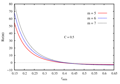
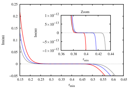
Figure 4: Real (left) and imaginary (right) components of the fundamental QNM frequencies, plotted as a function of $r_{\rm min}$, for $C=0.5$ and $m=5,\,6,\,7$. These results were obtained via the CF method.

From the results exhibited in Table 5.2, it can be seen that as the azimuthal number $m$ increases, the magnitude of the real (imaginary) part of the QNM frequencies increases (decreases). Moreover, from the plots exhibited in Fig. 4, we find that as $r_{\rm min}$ decreases, the magnitude of the real and imaginary parts of the QNM frequencies increase (decrease) for unstable (stable) modes. This behavior of the imaginary part can be clearly seen in the inset of the right panel of Fig. 4.

5.3 Acoustic clouds

As analogues to the clouds around rotating BHs, described in Section 4.3.2, we may have acoustic clouds around the draining bathtub. Taking advantage of the symmetries of the draining bathtub spacetime, characterized by Eq. (44), we can search for solutions of the Klein-Gordon equation (41), assuming the separation of variables

$$\Phi_{m}(r,\phi,t)=e^{i(m\phi-\omega t)}\zeta_{m}(r).$$ (53)

The radial function $\zeta_{m}(r)$ obeys the ordinary differential equation

$$\frac{h(r)}{r}\frac{d}{dr}\left[rh(r)\frac{d\zeta_{m}}{dr}\right]+\left[\omega^{2}-\frac{2Cm\omega}{r^{2}}-\frac{m^{2}}{r^{2}}\left(1-\frac{D^{2}+C^{2}}{r^{2}}\right)\right]\zeta_{m}=0.$$ (54)

Using the tortoise coordinate, defined by

$$\frac{d}{dr_{*}}\equiv h(r)\frac{d}{dr}\,,$$ (55)

we can rewrite Eq. (54) as the Schrödinger-like equation

$$\frac{d^{2}}{dr_{*}^{2}}u_{m}+\left[\left(\omega-\frac{Cm}{r^{2}}\right)^{2}-V^{\text{dbt}}_{m}(r)\right]u_{m}=0\ ,$$ (56)

where $u_{m}\equiv\sqrt{r}\zeta_{m}$, and we have defined the effective potential

$$V^{\text{dbt}}_{m}(r)=h(r)\left[\frac{m^{2}-1/4}{r^{2}}+\frac{5D^{2}}{4r^{2}}\right]\ .$$ (57)

Considering the asymptotic limit of Eq. (56), we find the solutions

$$\zeta_{\omega m}(r)\sim\left\{\begin{array}[]{ll}e^{-i(\omega-\omega_{c})r_{*}},&\mbox{for $r\rightarrow r_{H}$}\ ,\\ e^{i\omega r_{*}},&\mbox{for $r\rightarrow\infty$}\ .\end{array}\right.$$ (58)

In order to have clouds we must choose $\omega=\omega_{c}\equiv m\Omega_{H}$, and enclose the system inside a “barrier” located at $r=r_{0}$. At the “barrier” we impose suitable boundary conditions, usually chosen to be of Dirichlet or Neumann type. [302]

In Fig. 5 we analyze the behavior of the acoustic clouds by plotting the values of the frontier location $r_{0}$ as a function of the angular velocity at the horizon $\Omega_{H}$, for different choices of the azimuthal number $m$. We see that, for a fixed position $r_{0}$ of the barrier, the acoustic clouds occur for smaller values of $\Omega_{H}$ as we increase the value of $m$.

Three-dimensional plots of the radial and azimuthal profiles of acoustic clouds are shown in Fig. 6, for Dirichlet (left panel) and Neumann (right panel) boundary conditions.

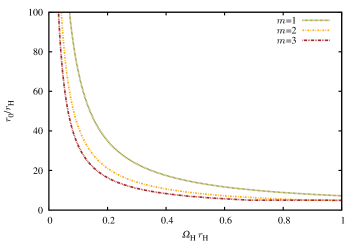
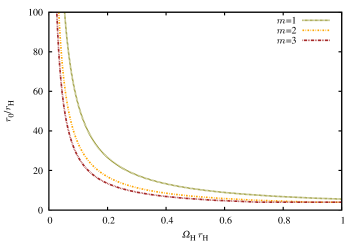
Figure 5: Acoustic clouds around the draining bathtub surrounded by a boundary at $r=r_{0}$, with angular velocity at the horizon $\Omega_{H}$, for $n=1$ and different values of $m$, for Dirichlet (left panel) and Neumann (right panel) boundary conditions. The number $n$ denotes the node number of the radial function. Similar figures, but with different choices of the clouds quantum numbers can be found in Benone et al. [304, 305]

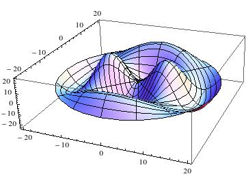
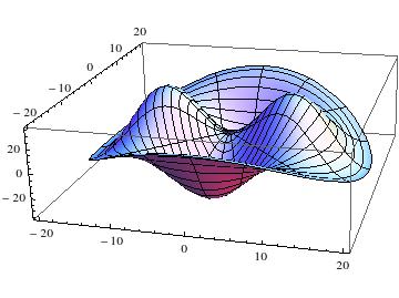
Figure 6: Real part of $\Phi$ in the $x,y$ plane, for $r_{0}/r_{H}=20$, $n=1$ and $m=2$. The left panel displays the case for Dirichlet boundary conditions, with $C/r_{H}=0.21$, while the right panel displays the case for Neumann boundary conditions, with $C/r_{H}=0.17$.

6 Concluding Remarks

The fantastic conceptual and formal elegance of Einstein’s gravity hides a tremendous complexity when it is applied to realistic, dynamical systems. Quite often, all hope of finding elegant analytic solutions is lost. Then, to tackle this complexity, one needs to resort to numerical solutions. This necessity is now well understood by the scientific community and with the current available techniques, together with the ones under development, there is a strong belief that a lot can be learned about the most elegant physical theory – or generalizations thereof – in the strong field, dynamical regime. We foresee interesting times ahead.

References

- [1] B. . Abbott et al., Phys. Rev. Lett. 116 (2016) 061102, arXiv:1602.03837 [gr-qc].
- [2] F. Pretorius, Phys. Rev. Lett. 95 (2005) 121101, arXiv:gr-qc/0507014.
- [3] J. G. Baker, J. M. Centrella, D.-I. Choi, M. Koppitz and J. R. van Meter, Phys. Rev. Lett. 96 (2006) 111102, arXiv:gr-qc/0511103.
- [4] M. Campanelli, C. O. Lousto, P. Marronetti and Y. Zlochower, Phys. Rev. Lett. 96 (2006) 111101, arXiv:gr-qc/0511048.
- [5] V. Cardoso et al., Class. Quant. Grav. 29 (2012) 244001, arXiv:1201.5118 [hep-th].
- [6] E. Berti et al., Class. Quant. Grav. 32 (2015) 243001, arXiv:1501.07274 [gr-qc].
- [7] V. Cardoso, L. Gualtieri, C. Herdeiro and U. Sperhake, Living Rev. Relativ. 18 (2015) arXiv:1409.0014 [gr-qc].
- [8] U. Sperhake, Gen. Rel. Grav. 46 (2014) 1689.
- [9] L. Blanchet, Living Reviews in Relativity 9 (2006) http://www.livingreviews.org/lrr-2006-4.
- [10] M. Sasaki and H. Tagoshi, Living Rev. Relativ. 6 (2003) arXiv:gr-qc/0306120.
- [11] E. Poisson, A. Pound and I. Vega, Living Rev. Relativ. 14 (2011) 7, arXiv:1102.0529 [gr-qc].
- [12] M. Alcubierre, Introduction to 3+1 Numerical Relativity (Oxford University Press, 2008).
- [13] C. Bona, C. Palenzuela-Luque and C. Bona-Casas, Elements of Numerical Relativity and Relativistic Hydrodynamics (Springer Dordrecht Heidelberg London New York, 2009).
- [14] T. W. Baumgarte and S. L. Shapiro, Numerical Relativity (Cambridge University Press, 2010).
- [15] U. Sperhake, Class. Quantum Grav. 32 (2015) 124011, arXiv:1411.3997 [gr-qc].
- [16] P. C. Peters, Phys. Rev. 136 (1964) B1224.
- [17] C. W. Lincoln and C. M. Will, Phys. Rev. D42 (1990) 1123.
- [18] T. Mora and C. M. Will, Phys. Rev. D69 (2004) 104021, arXiv:gr-qc/0312082 [gr-qc].
- [19] T. Damour, A. Gopakumar and B. R. Iyer, Phys. Rev. D70 (2004) 064028, arXiv:gr-qc/0404128 [gr-qc].
- [20] I. Hinder, B. Vaishnav, F. Herrmann, D. M. Shoemaker and P. Laguna, Phys. Rev. D77 (2008) 081502, arXiv:0710.5167 [gr-qc].
- [21] U. Sperhake, E. Berti, V. Cardoso, J. A. González, B. Brügmann and M. Ansorg, Phys. Rev. D78 (2008) 064069, arXiv:0710.3823 [gr-qc].
- [22] I. Hinder, F. Herrmann, P. Laguna and D. M. Shoemaker, Phys. Rev. D82 (2010) 024033, arXiv:0806.1037 [gr-qc].
- [23] N. Yunes, K. Arun, E. Berti and C. M. Will, Phys. Rev. D80 (2009) 084001, arXiv:0906.0313 [gr-qc].
- [24] E. Huerta and D. A. Brown (2013) arXiv:1301.1895 [gr-qc].
- [25] E. Huerta, P. Kumar, S. T. McWilliams, R. O’Shaughnessy and N. Yunes, Phys. Rev. D90 (2014) 084016, arXiv:1408.3406 [gr-qc].
- [26] C. K. Mishra, K. G. Arun and B. R. Iyer, Phys. Rev. D 91 (2015) 084040, arXiv:1501.07096 [gr-qc].
- [27] E. Berti, V. Cardoso, L. Gualtieri, M. Horbatsch and U. Sperhake, Phys. Rev. D87 (2013) 124020, arXiv:1304.2836 [gr-qc].
- [28] J. Healy, T. Bode, R. Haas, E. Pazos, P. Laguna et al., Class. Quantum Grav. 29 (2012) 232002, arXiv:1112.3928 [gr-qc].
- [29] É. É. Flanagan and S. A. Hughes, Phys. Rev. D57 (1998) 4566, arXiv:gr-qc/9710129.
- [30] The LIGO Scientific Collaboration, the Virgo Collaboration, the NINJA-2 Collaboration Collaboration (J. Aasi et al.), Class.Quant.Grav. 31 (2014) 115004, arXiv:1401.0939 [gr-qc].
- [31] P. Ajith, M. Boyle, D. A. Brown, B. Brugmann, L. T. Buchman et al. (2012) arXiv:1201.5319 [gr-qc].
- [32] I. Hinder et al., Class. Quant. Grav. 31 (2014) 025012, arXiv:1307.5307 [gr-qc].
- [33] S. Khan et al., Phys. Rev. D 93 (2016) 044007, arXiv:1508.07253 [gr-qc].
- [34] Y. Pan, A. Buonanno, A. Taracchini, L. E. Kidder, A. H. Mroue et al., Phys. Rev. D 89 (2014) 084006, arXiv:1307.6232 [gr-qc].
- [35] A. Taracchini et al., Phys. Rev. D 89 (2014) 061502, arXiv:1311.2544 [gr-qc].
- [36] T. Damour and A. Nagar, Phys. Rev. D 90 (2014) 044018, arXiv:1406.6913 [gr-qc].
- [37] A. Nagar, T. Damour, C. Reisswig and D. Pollney (2015) arXiv:1506.08457 [gr-qc].
- [38] T. A. Apostolatos, C. Cutler, G. J. Sussman and K. S. Thorne, Phys. Rev. D49 (1994) 6274.
- [39] L. E. Kidder, Phys. Rev. D52 (1995) 821, arXiv:gr-qc/9506022.
- [40] K. G. Arun, A. Buonanno, G. Faye and E. Ochsner, Phys. Rev. D79 (2009) 104023, arXiv:0810.5336 [gr-qc].
- [41] T. A. Apostolatos, Phys. Rev. D52 (1995) 605.
- [42] M. Hannam, P. Schmidt, A. Bohé, L. Haegel, S. Husa et al., Phys. Rev. Lett. 113 (2014) 151101, arXiv:1308.3271 [gr-qc].
- [43] A. Klein, N. Cornish and N. Yunes, Phys. Rev. D 88 (2013) 124015, arXiv:1305.1932 [gr-qc].
- [44] A. Klein, N. Cornish and N. Yunes, Phys. Rev. D 90 (2014) 124029, arXiv:1408.5158 [gr-qc].
- [45] A. Lundgren and R. O’Shaughnessy, Phys. Rev. D89 (2014) 044021, arXiv:1304.3332 [gr-qc].
- [46] P. Schmidt, F. Ohme and M. Hannam, Phys. Rev. D91 (2015) 024043, arXiv:1408.1810 [gr-qc].
- [47] J. D. Schnittman, Phys. Rev. D70 (2004) 124020, arXiv:astro-ph/0409174 [astro-ph].
- [48] M. Kesden, U. Sperhake and E. Berti, Phys. Rev. D81 (2010) 084054, arXiv:1002.2643 [astro-ph.GA].
- [49] M. Kesden, U. Sperhake and E. Berti, Astrophys. J. 715 (2010) 1006, arXiv:1003.4993 [astro-ph.CO].
- [50] E. Berti, M. Kesden and U. Sperhake, Phys. Rev. D 85 (2012) 124049, arXiv:1203.2920 [astro-ph].
- [51] M. Kesden, D. Gerosa, R. O’Shaughnessy, E. Berti and U. Sperhake, Phys. Rev. Lett. 114 (2015) 081103, arXiv:1411.0674 [gr-qc].
- [52] D. Gerosa, M. Kesden, U. Sperhake, E. Berti and R. O’Shaughnessy, Phys. Rev. D92 (2015) 064016, arXiv:1506.03492 [gr-qc].
- [53] T. Damour, Phys. Rev. D64 (2001) 124013, arXiv:gr-qc/0103018.
- [54] E. Racine, Phys. Rev. D 78 (2008) 044021, arXiv:0803.1820 [gr-qc].
- [55] D. Gerosa, M. Kesden, R. O’Shaughnessy, A. Klein, E. Berti, U. Sperhake and D. Trifirò, Phys. Rev. Lett. 115 (2015) 141102, arXiv:1506.09116 [gr-qc].
- [56] D. Gerosa, M. Kesden, E. Berti, R. O’Shaughnessy and U. Sperhake, Phys. Rev. D 87 (2013) 104028, arXiv:1302.4442 [gr-qc].
- [57] D. Gerosa, R. O’Shaughnessy, M. Kesden, E. Berti and U. Sperhake, Phys. Rev. D89 (2014) 124025, arXiv:1403.7147 [gr-qc].
- [58] D. Trifirò, R. O’Shaughnessy, D. Gerosa, E. Berti, M. Kesden, T. Littenberg and U. Sperhake (2015) arXiv:1507.05587 [gr-qc].
- [59] R. Penrose, Phys. Rev. Lett. 14 (1965) 57.
- [60] S. Hawking, Proc. Roy. Soc. Lond. A300 (1967) 187.
- [61] S. Hawking and R. Penrose, Proc.Roy.Soc.Lond. A314 (1970) 529.
- [62] R. M. Wald, Gravitational collapse and cosmic censorship, in In *Iyer, B. R. (ed.) et al.: Black holes, gravitational radiation and the universe* 69-85, (Springer Science+Business Media, Dordrecht, 1997). gr-qc/9710068.
- [63] K. Thorne, Nonspherical gravitational collapse: A short review, in Magic Without Magic, ed. J. Klauder (Freeman, San Francisco, 1972), p. 231.
- [64] D. Ida and K.-i. Nakao, Phys. Rev. D 66 (2002) 064026, gr-qc/0204082.
- [65] M. W. Choptuik and F. Pretorius, Phys. Rev. Lett. 104 (2010) 111101, arXiv:0908.1780 [gr-qc].
- [66] I. Antoniadis, N. Arkani-Hamed, S. Dimopoulos and G. R. Dvali, Phys. Lett. B436 (1998) 257, arXiv:hep-ph/9804398.
- [67] N. Arkani-Hamed, S. Dimopoulos and G. R. Dvali, Phys. Lett. B429 (1998) 263, arXiv:hep-ph/9803315.
- [68] L. Randall and R. Sundrum, Phys. Rev. Lett. 83 (1999) 3370, arXiv:hep-ph/9905221.
- [69] L. Randall and R. Sundrum, Phys. Rev. Lett. 83 (1999) 4690, arXiv:hep-th/9906064.
- [70] S. Dimopoulos and G. Landsberg, Phys. Rev. Lett. 87 (2001) 161602, hep-th/0106295.
- [71] S. B. Giddings and S. Thomas, Phys. Rev. D 65 (2002) 056010, hep-ph/0106219.
- [72] J. A. Frost, J. R. Gaunt, M. O. P. Sampaio, M. Casals, S. R. Dolan et al., JHEP 10 (2009) 014, arXiv:0904.0979 [hep-th].
- [73] J. M. Maldacena, Adv. Theor. Math. Phys. 2 (1998) 231, arXiv:hep-th/9711200.
- [74] S. S. Gubser, I. R. Klebanov and A. M. Polyakov, Phys. Lett. B428 (1998) 105, arXiv:hep-th/9802109.
- [75] E. Witten, Adv. Theor. Math. Phys. 2 (1998) 253, arXiv:hep-th/9802150.
- [76] F. Pretorius, Binary Black Hole Coalescence, in Physics of relativistic objects in compact binaries: from birth to coalescence (Astrophysics and Space Science Library, Vol. 359), (Springer, New York, 2007), New York, ch. 9.
- [77] U. Sperhake, E. Berti and V. Cardoso, Comptes Rendus Physique 14 (2013) 306, arXiv:1107.2819 [gr-qc].
- [78] W. E. East and F. Pretorius, Phys. Rev. Lett. 110 (2013) 101101, arXiv:1210.0443 [gr-qc].
- [79] L. Rezzolla and K. Takami, Class. Quant. Grav. 30 (2013) 012001, arXiv:1209.6138 [gr-qc].
- [80] U. Sperhake, V. Cardoso, F. Pretorius, E. Berti and J. A. González, Phys. Rev. Lett. 101 (2008) 161101, arXiv:0806.1738 [gr-qc].
- [81] J. Healy, I. Ruchlin and C. O. Lousto (2015) arXiv:1506.06153 [gr-qc].
- [82] R. Penrose, (1974), presented at the Cambridge University Seminar, Cambridge, England (unpublished).
- [83] D. M. Eardley and S. B. Giddings, Phys. Rev. D66 (2002) 044011, arXiv:gr-qc/0201034 [gr-qc].
- [84] P. D. D’Eath, Phys. Rev. D 18 (1978) 990.
- [85] P. D. D’Eath and P. N. Payne, Phys. Rev. D46 (1992) 658.
- [86] P. D. D’Eath and P. N. Payne, Phys. Rev. D46 (1992) 675.
- [87] C. Herdeiro, M. O. P. Sampaio and C. Rebelo, JHEP 1107 (2011) 121, arXiv:1105.2298i [hep-th].
- [88] F. S. Coelho, C. Herdeiro and M. O. P. Sampaio, Phys. Rev. Lett. 108 (2012) 181102, arXiv:1203.5355 [hep-th].
- [89] F. S. Coelho, C. Herdeiro, C. Rebelo and M. Sampaio, Phys. Rev. D87 (2013) 084034, arXiv:1206.5839 [hep-th].
- [90] F. S. Coelho, C. Herdeiro, C. Rebelo and M. O. P. Sampaio, Radiation from a D-dimensional collision of shock waves: an insight allowed by the D parameter, in Proceedings, 13th Marcel Grossmann Meeting on Recent Developments in Theoretical and Experimental General Relativity, Astrophysics, and Relativistic Field Theories (MG13), (2015), pp. 1059–1061. arXiv:1301.1073 [gr-qc].
- [91] F. S. Coelho, C. Herdeiro and M. O. P. Sampaio, JHEP 12 (2014) 119, arXiv:1410.0964 [hep-th].
- [92] F. d. S. Coelho, Radiation from a -dimensional collision of gravitational shock waves, PhD thesis, Aveiro U. (2015).
- [93] M. Shibata, H. Okawa and T. Yamamoto, Phys. Rev. D78 (2008) 101501, arXiv:0810.4735 [gr-qc].
- [94] U. Sperhake, V. Cardoso, F. Pretorius, E. Berti, T. Hinderer and N. Yunes, Phys. Rev. Lett. 103 (2009) 131102, arXiv:0907.1252 [gr-qc].
- [95] F. Pretorius and D. Khurana, Class. Quantum Grav. 24 (2007) S83, arXiv:gr-qc/0702084.
- [96] U. Sperhake, E. Berti, V. Cardoso and F. Pretorius, Phys. Rev. Lett. 111 (2013) 041101, arXiv:1211.6114 [gr-qc].
- [97] U. Sperhake, E. Berti, V. Cardoso and F. Pretorius, Phys. Rev. D 93 (2016) 044012, arXiv:1511.08209 [gr-qc].
- [98] M. Zilhao, V. Cardoso, C. Herdeiro, L. Lehner and U. Sperhake, Phys. Rev. D 85 (2012) 124062, arXiv:1205.1063 [gr-qc].
- [99] M. Zilhão, V. Cardoso, C. Herdeiro, L. Lehner and U. Sperhake, Phys. Rev. D 89 (2014) 044008, arXiv:1311.6483 [gr-qc].
- [100] T. Piran, J. Shaham and J. Katz, Astrophys. J. 196 (Mar 1975) L107.
- [101] M. Banados, J. Silk and S. M. West, Phys. Rev. Lett. 103 (2009) 111102, arXiv:0909.0169 [hep-th].
- [102] E. Berti, V. Cardoso, L. Gualtieri, F. Pretorius and U. Sperhake, Phys. Rev. Lett. 103 (2009) 239001, arXiv:0911.2243 [gr-qc].
- [103] T. Jacobson and T. P. Sotiriou, Phys. Rev. Lett. 104 (2010) 021101, arXiv:0911.3363 [gr-qc].
- [104] S. T. McWilliams, Phys. Rev. Lett. 110 (2013) 011102, arXiv:1212.1235 [gr-qc].
- [105] T. Piran and J. Shaham, Phys. Rev. D 16 (1977) 1615.
- [106] T. Harada, H. Nemoto and U. Miyamoto, Phys. Rev. D 86 (2012) 024027, 1205.7088, [Erratum: Phys. Rev.D86,069902(2012)].
- [107] J. D. Schnittman, Phys. Rev. Lett. 113 (2014) 261102, arXiv:1410.6446 [astro-ph].
- [108] E. Berti, R. Brito and V. Cardoso, Phys. Rev. Lett. 114 (2015) 251103, arXiv:1410.8534 [gr-qc].
- [109] K. Ogasawara, T. Harada and U. Miyamoto, Phys. Rev. D93 (2016) 044054, arXiv:1511.00110 [gr-qc].
- [110] E. Leiderschneider and T. Piran, Phys. Rev. D93 (2016) 043015, arXiv:1510.06764 [gr-qc].
- [111] H. Okawa, K.-i. Nakao and M. Shibata, Phys. Rev. D 83 (2011) 121501, arXiv:1105.3331 [gr-qc].
- [112] M. Alcubierre, S. Brandt, B. Brügmann, D. Holz, E. Seidel, R. Takahashi and J. Thornburg, Int. J. Mod. Phys. D 10 (2001) 273, gr-qc/9908012.
- [113] F. Pretorius, Class. Quantum Grav. 22 (2005) 425, gr-qc/0407110.
- [114] H. Yoshino and M. Shibata, Prog.Theor.Phys.Suppl. 189 (2011) 269.
- [115] H. Yoshino and M. Shibata, Prog.Theor.Phys.Suppl. 190 (2011) 282.
- [116] W. G. Cook, P. Figueras, M. Kunesch, U. Sperhake and S. Tunyasuvunakool, Dimensional reduction in numerical relativity: Modified cartoon formalism and regularization, in 3rd Amazonian Symposium on Physics and 5th NRHEP Network Meeting: Celebrating 100 Years of General Relativity Belem, Brazil, September 28-October 2, 2015, (2016). arXiv:1603.00362 [gr-qc].
- [117] H. Witek, M. Zilhão, L. Gualtieri, V. Cardoso, C. Herdeiro, A. Nerozzi and U. Sperhake, Phys. Rev. D82 (2010) 104014, arXiv:1006.3081 [gr-qc].
- [118] H. Witek, V. Cardoso, L. Gualtieri, C. Herdeiro, U. Sperhake and M. Zilhão, Phys. Rev. D83 (2011) 044017, arXiv:1011.0742 [gr-qc].
- [119] M. Zilhao, H. Witek, U. Sperhake, V. Cardoso, L. Gualtieri, C. Herdeiro and A. Nerozzi, Phys. Rev. D81 (2010) 084052, arXiv:1001.2302 [gr-qc].
- [120] R. Geroch, J. Math. Phys. 12 (1970) 918.
- [121] H. Witek, H. Okawa, V. Cardoso, L. Gualtieri, C. Herdeiro, M. Shibata, U. Sperhake and M. Zilhão, Phys. Rev. D 90 (2014) 084014, arXiv:1406.2703 [gr-qc].
- [122] H. Yoshino and Y. Nambu, Phys. Rev. D 67 (2003) 024009, gr-qc/0209003.
- [123] H. Yoshino and V. S. Rychkov, Phys. Rev. D 71 (2005) 104028, hep-th/0503171.
- [124] H. Bantilan, F. Pretorius and S. S. Gubser, Phys. Rev. D 85 (2012) 084038, arXiv:1201.2132 [hep-th].
- [125] P. M. Chesler and L. G. Yaffe, JHEP 1407 (2014) 086, arXiv:1309.1439 [hep-th].
- [126] H. Bantilan and P. Romatschke, Phys. Rev. Lett. 114 (2015) 081601, arXiv:1410.4799 [hep-th].
- [127] H. Witek, V. Cardoso, C. Herdeiro, A. Nerozzi, U. Sperhake and M. Zilhão, Phys. Rev. D82 (2010) 104037, arXiv:1004.4633 [hep-th].
- [128] P. M. Chesler and L. G. Yaffe, Phys. Rev. Lett. 102 (2009) 211601, arXiv:0812.2053 [hep-th].
- [129] P. M. Chesler and L. G. Yaffe, Phys. Rev. Lett. 106 (2011) 021601, arXiv:1011.3562 [hep-th].
- [130] M. P. Heller, R. A. Janik and P. Witaszczyk, Phys. Rev. D 85 (2012) 126002, arXiv:1203.0755 [hep-th].
- [131] M. P. Heller, D. Mateos, W. van der Schee and D. Trancanelli, Phys. Rev. Lett. 108 (2012) 191601, arXiv:1202.0981 [hep-th].
- [132] V. Cardoso, R. Emparan, D. Mateos, P. Pani and J. V. Rocha, JHEP 01 (2014) 138, arXiv:1310.7590 [hep-th].
- [133] M. Zilhao, V. Cardoso, L. Gualtieri, C. Herdeiro, U. Sperhake and H. Witek, Phys. Rev. D85 (2012) 104039, arXiv:1204.2019 [gr-qc].
- [134] T. Damour and G. Esposito-Farése, Class. Quantum Grav. 9 (1992) 2093.
- [135] T. Chiba, T. Harada and K.-i. Nakao, Prog. Theor. Phys. Suppl. 128 (1997) 335.
- [136] Y. Fujii and K.-I. Maeda, The Scalar-Tensor Theory of Gravitation (Cambridge University Press, March 2003).
- [137] V. Faraoni, Cosmology in scalar tensor gravity (Springer, 2004).
- [138] C. A. R. Herdeiro and E. Radu, Int. J. Mod. Phys. D24 (2015) 1542014, arXiv:1504.08209 [gr-qc].
- [139] T. P. Sotiriou, Lect. Notes Phys. 892 (2015) 3, arXiv:1404.2955 [gr-qc].
- [140] P. G. Bergmann, Int. J. Theor. Phys. 1 (1968) 25.
- [141] R. V. Wagoner, Phys. Rev. D1 (1970) 3209.
- [142] P. Jordan, Z. Phys. 157 (1959) 112.
- [143] M. Fierz, Helv. Phys. Acta 29 (1956) 128.
- [144] C. Brans and R. Dicke, Phys. Rev. 124 (1961) 925.
- [145] E. E. Flanagan, Class. Quantum Grav. 21 (2004) 3817, arXiv:gr-qc/0403063 [gr-qc].
- [146] T. P. Sotiriou, S. Liberati and V. Faraoni, Int. J. Mod. Phys. D17 (2008) 399, arXiv:0707.2748 [gr-qc].
- [147] C. M. Will, Living Rev. Relativ. 17 (2014) 4, arXiv:1403.7377 [gr-qc].
- [148] J. Alsing, E. Berti, C. M. Will and H. Zaglauer, Phys. Rev. D85 (2012) 064041, arXiv:1112.4903 [gr-qc].
- [149] T. Damour and G. Esposito-Farèse, Phys. Rev. Lett. 70 (1993) 2220.
- [150] T. Damour and G. Esposito-Farese, Phys. Rev. D54 (1996) 1474, arXiv:gr-qc/9602056 [gr-qc].
- [151] T. Damour and G. Esposito-Farese, Phys. Rev. D53 (1996) 5541, arXiv:gr-qc/9506063 [gr-qc].
- [152] C. M. Will, Living Rev. Rel. 9 (2006) 3, arXiv:gr-qc/0510072 [gr-qc].
- [153] D. M. Eardley, Astrophys. J. 196 (1975) L59.
- [154] C. M. Will and H. W. Zaglauer, Astrophys. J. 346 (1989) 366.
- [155] P. C. Freire, N. Wex, G. Esposito-Farese, J. P. Verbiest, M. Bailes et al., Mon. Not. R. Astron. Soc. 423 (2012) 3328, arXiv:1205.1450 [astro-ph.GA].
- [156] N. Yunes, P. Pani and V. Cardoso, Phys. Rev. D85 (2012) 102003, arXiv:1112.3351 [gr-qc].
- [157] T. Damour and G. Esposito-Farese, Phys. Rev. D58 (1998) 042001, arXiv:gr-qc/9803031 [gr-qc].
- [158] R. F. P. Mendes, Phys. Rev. D91 (2015) 064024, arXiv:1412.6789 [gr-qc].
- [159] C. Palenzuela and S. L. Liebling, Phys. Rev. D93 (2016) 044009, arXiv:1510.03471 [gr-qc].
- [160] T. Harada, Phys. Rev. D57 (1998) 4802, arXiv:gr-qc/9801049.
- [161] M. Salgado, D. Sudarsky and U. Nucamendi, Phys. Rev. D58 (1998) 124003, arXiv:gr-qc/9806070 [gr-qc].
- [162] M. Shibata, K. Nakao and T. Nakamura, Phys. Rev. D50 (1994) 7304.
- [163] T. Harada, T. Chiba, K.-i. Nakao and T. Nakamura, Phys. Rev. D55 (1997) 2024, arXiv:gr-qc/9611031 [gr-qc].
- [164] J. Novak, Phys. Rev. D57 (1998) 4789, arXiv:gr-qc/9707041 [gr-qc].
- [165] D. Gerosa, U. Sperhake and C. D. Ott (2016) arXiv:1602.06952 [gr-qc].
- [166] T. Harada, Prog. Theor. Phys. 98 (1997) 359, arXiv:gr-qc/9706014 [gr-qc].
- [167] W. C. Lima, G. E. Matsas and D. A. Vanzella, Phys. Rev. Lett. 105 (2010) 151102, arXiv:1009.1771 [gr-qc].
- [168] P. Pani, V. Cardoso, E. Berti, J. Read and M. Salgado, Phys. Rev. D83 (2011) 081501, arXiv:1012.1343 [gr-qc].
- [169] R. F. Mendes, G. E. Matsas and D. A. Vanzella, Phys. Rev. D89 (2014) 047503, arXiv:1310.2185 [gr-qc].
- [170] A. G. S. Landulfo, W. C. C. Lima, G. E. A. Matsas and D. A. T. Vanzella, Phys. Rev. D91 (2015) 024011, arXiv:1410.2274 [gr-qc].
- [171] H. Sotani and K. D. Kokkotas, Phys. Rev. D70 (2004) 084026, arXiv:gr-qc/0409066 [gr-qc].
- [172] H. Sotani and K. D. Kokkotas, Phys. Rev. D71 (2005) 124038, arXiv:gr-qc/0506060 [gr-qc].
- [173] H. Sotani, Phys. Rev. D89 (2014) 064031, arXiv:1402.5699 [astro-ph.HE].
- [174] H. O. Silva, H. Sotani, E. Berti and M. Horbatsch, Phys. Rev. D90 (2014) 124044, arXiv:1410.2511 [gr-qc].
- [175] F. M. Ramazanoglu and F. Pretorius, Phys. Rev. D 93 (2016) 064005, arXiv:1601.07475 [gr-qc].
- [176] P. Pani and E. Berti, Phys. Rev. D90 (2014) 024025, arXiv:1405.4547 [gr-qc].
- [177] H. Sotani, Phys. Rev. D86 (2012) 124036, arXiv:1211.6986 [astro-ph.HE].
- [178] D. D. Doneva, S. S. Yazadjiev, N. Stergioulas and K. D. Kokkotas, Phys. Rev. D88 (2013) 084060, arXiv:1309.0605 [gr-qc].
- [179] N. Stergioulas, Living Rev. Relativ. 6 (2003) 3, arXiv:gr-qc/0302034 [gr-qc].
- [180] D. D. Doneva, S. S. Yazadjiev, N. Stergioulas, K. D. Kokkotas and T. M. Athanasiadis, Phys. Rev. D90 (2014) 044004, arXiv:1405.6976 [astro-ph.HE].
- [181] D. D. Doneva, S. S. Yazadjiev, K. V. Staykov and K. D. Kokkotas, Phys. Rev. D90 (2014) 104021, arXiv:1408.1641 [gr-qc].
- [182] E. Barausse, C. Palenzuela, M. Ponce and L. Lehner, Phys. Rev. D87 (2013) 081506, arXiv:1212.5053 [gr-qc].
- [183] C. Palenzuela, E. Barausse, M. Ponce and L. Lehner, Phys. Rev. D89 (2014) 044024, arXiv:1310.4481 [gr-qc].
- [184] M. Shibata, K. Taniguchi, H. Okawa and A. Buonanno, Phys. Rev. D89 (2014) 084005, arXiv:1310.0627 [gr-qc].
- [185] K. Taniguchi, M. Shibata and A. Buonanno, Phys. Rev. D91 (2015) 024033, arXiv:1410.0738 [gr-qc].
- [186] L. Sampson, N. Yunes, N. Cornish, M. Ponce, E. Barausse et al., Phys. Rev. D90 (2014) 124091, arXiv:1407.7038 [gr-qc].
- [187] H. O. Silva, C. F. B. Macedo, E. Berti and L. C. B. Crispino, Class. Quant. Grav. 32 (2015) 145008, arXiv:1411.6286 [gr-qc].
- [188] S. G. Nelmes and B. M. A. G. Piette, Phys. Rev. D85 (2012) 123004, arXiv:1204.0910 [astro-ph.SR].
- [189] C. Adam, C. Naya, J. Sanchez-Guillen, R. Vazquez and A. Wereszczynski, Phys. Lett. B742 (2015) 136, arXiv:1407.3799 [hep-th].
- [190] C. Adam, C. Naya, J. Sanchez-Guillen, R. Vazquez and A. Wereszczynski, Phys. Rev. C92 (2015) 025802, arXiv:1503.03095 [nucl-th].
- [191] R. L. Bowers and E. P. T. Liang, Astrophys. J. 188 (March 1974) 657.
- [192] K. Yagi and N. Yunes, Phys. Rev. D91 (2015) 103003, arXiv:1502.04131 [gr-qc].
- [193] K. Yagi and N. Yunes, Phys. Rev. D91 (2015) 123008, arXiv:1503.02726 [gr-qc].
- [194] K. Yagi and N. Yunes (2016) arXiv:1601.02171 [gr-qc].
- [195] S. Hawking, Commun. Math. Phys. 25 (1972) 167.
- [196] M. Heusler, Class. Quantum Grav. 12 (1995) 2021, arXiv:gr-qc/9503053 [gr-qc].
- [197] T. P. Sotiriou and V. Faraoni, Phys. Rev. Lett. 108 (2012) 081103, arXiv:1109.6324 [gr-qc].
- [198] S. Mirshekari and C. M. Will, Phys. Rev. D87 (2013) 084070, arXiv:1301.4680 [gr-qc].
- [199] C. A. R. Herdeiro and E. Radu, Phys. Rev. Lett. 112 (2014) 221101, arXiv:1403.2757 [gr-qc].
- [200] C. Herdeiro and E. Radu, Class. Quantum Grav. 32 (2015) 144001, arXiv:1501.04319 [gr-qc].
- [201] M. Horbatsch, H. O. Silva, D. Gerosa, P. Pani, E. Berti, L. Gualtieri and U. Sperhake, Class. Quant. Grav. 32 (2015) 204001, arXiv:1505.07462 [gr-qc].
- [202] G. W. Horndeski, Int. J. Theor. Phys. 10 (1974) 363.
- [203] C. Deffayet, X. Gao, D. Steer and G. Zahariade, Phys. Rev. D84 (2011) 064039, arXiv:1103.3260 [hep-th].
- [204] T. Kobayashi, M. Yamaguchi and J. Yokoyama, Prog. Theor. Phys. 126 (2011) 511, arXiv:1105.5723 [hep-th].
- [205] A. Maselli, H. O. Silva, M. Minamitsuji and E. Berti, Phys. Rev. D92 (2015) 104049, arXiv:1508.03044 [gr-qc].
- [206] C. Charmousis, E. J. Copeland, A. Padilla and P. M. Saffin, Phys. Rev. Lett. 108 (2012) 051101, arXiv:1106.2000 [hep-th].
- [207] C. Charmousis, E. J. Copeland, A. Padilla and P. M. Saffin, Phys. Rev. D85 (2012) 104040, arXiv:1112.4866 [hep-th].
- [208] T. Kobayashi and N. Tanahashi, PTEP 2014 (2014) 073E02, arXiv:1403.4364 [gr-qc].
- [209] C. Armendariz-Picon, V. F. Mukhanov and P. J. Steinhardt, Phys. Rev. D63 (2001) 103510, arXiv:astro-ph/0006373 [astro-ph].
- [210] C. Armendariz-Picon, T. Damour and V. F. Mukhanov, Phys. Lett. B458 (1999) 209, arXiv:hep-th/9904075 [hep-th].
- [211] M. Alishahiha, E. Silverstein and D. Tong, Phys. Rev. D70 (2004) 123505, arXiv:hep-th/0404084 [hep-th].
- [212] C. Deffayet, G. Esposito-Farese and A. Vikman, Phys. Rev. D79 (2009) 084003, arXiv:0901.1314 [hep-th].
- [213] H. O. Silva, A. Maselli, M. Minamitsuji and E. Berti, Compact objects in Horndeski gravity (2016). arXiv:1602.05997 [gr-qc].
- [214] P. Kanti, N. Mavromatos, J. Rizos, K. Tamvakis and E. Winstanley, Phys. Rev. D54 (1996) 5049, arXiv:hep-th/9511071 [hep-th].
- [215] T. P. Sotiriou and S.-Y. Zhou, Phys. Rev. Lett. 112 (2014) 251102, arXiv:1312.3622 [gr-qc].
- [216] N. Yunes and L. C. Stein, Phys. Rev. D83 (2011) 104002, arXiv:1101.2921 [gr-qc].
- [217] P. Pani, C. F. Macedo, L. C. Crispino and V. Cardoso, Phys. Rev. D84 (2011) 087501, arXiv:1109.3996 [gr-qc].
- [218] R. Jackiw and S. Y. Pi, Phys. Rev. D68 (2003) 104012, gr-qc/0308071.
- [219] S. Alexander and N. Yunes, Phys. Rept. 480 (2009) 1, arXiv:0907.2562 [hep-th].
- [220] R. P. Woodard, Lect. Notes Phys. 720 (2007) 403, arXiv:astro-ph/0601672 [astro-ph].
- [221] K. Stelle, Phys. Rev. D16 (1977) 953.
- [222] D. J. Gross and J. H. Sloan, Nucl. Phys. B291 (1987) 41.
- [223] F. Moura and R. Schiappa, Class. Quantum Grav. 24 (2007) 361, arXiv:hep-th/0605001.
- [224] P. Pani and V. Cardoso, Phys. Rev. D79 (2009) 084031, arXiv:0902.1569 [gr-qc].
- [225] K. Yagi, Phys. Rev. D86 (2012) 081504, arXiv:1204.4524 [gr-qc].
- [226] A. Maselli, L. Gualtieri, P. Pani, L. Stella and V. Ferrari, Astrophys. J. 801 (2015) 115, arXiv:1412.3473 [astro-ph.HE].
- [227] B. Kleihaus, J. Kunz and E. Radu, Phys. Rev. Lett. 106 (2011) 151104, arXiv:1101.2868 [gr-qc].
- [228] S. Mignemi and N. Stewart, Phys. Rev. D47 (1993) 5259, arXiv:hep-th/9212146 [hep-th].
- [229] D. Ayzenberg, K. Yagi and N. Yunes, Phys. Rev. D89 (2014) 044023, arXiv:1310.6392 [gr-qc].
- [230] A. Maselli, P. Pani, L. Gualtieri and V. Ferrari, Phys. Rev. D92 (2015) 083014, arXiv:1507.00680 [gr-qc].
- [231] M. Feroci, L. Stella, M. Van der Klis, T.-L. Courvoisier, M. Hernanz, R. Hudec, A. Santangelo, D. Walton, A. Zdziarski, D. Barret et al., Experimental Astronomy 34 (2012) 415.
- [232] R. Brito, V. Cardoso and P. Pani, Lect. Notes Phys. 906 (2015) pp.1, arXiv:1501.06570 [gr-qc].
- [233] D. J. E. Marsh and A.-R. Pop, Mon.Not.Roy.Astron.Soc. 451 (2015) 2479, arXiv:1502.03456 [astro-ph.CO].
- [234] H.-Y. Schive, T. Chiueh and T. Broadhurst, Nature Physics 10 (July 2014) 496, arXiv:1406.6586.
- [235] H.-Y. Schive, M.-H. Liao, T.-P. Woo, S.-K. Wong, T. Chiueh, T. Broadhurst and W.-Y. P. Hwang, Physical Review Letters 113 (December 2014) 261302, arXiv:1407.7762.
- [236] R. Brito, V. Cardoso and H. Okawa, Phys. Rev. Lett. 115 (2015) 111301, arXiv:1508.04773 [gr-qc].
- [237] R. Brito, V. Cardoso, C. F. B. Macedo, H. Okawa and C. Palenzuela, Phys. Rev. D93 (2016) 044045, arXiv:1512.00466 [astro-ph.SR].
- [238] M. W. Choptuik, Phys. Rev. Lett. 70 (1993) 9.
- [239] Y. B. Zel’dovich, Pis’ma Zh. Eksp. Teor. Fiz. 14 (1971) 270 [JETP Lett. 14, 180 (1971)].
- [240] Y. B. Zel’dovich, Zh. Eksp. Teor. Fiz 62 (1972) 2076 [Sov.Phys. JETP 35, 1085 (1972)].
- [241] V. Cardoso and P. Pani, Class. Quant. Grav. 30 (2013) 045011, arXiv:1205.3184 [gr-qc].
- [242] S. A. Teukolsky and W. H. Press, Astrophys. J. 193 (1974) 443.
- [243] W. H. Press and S. A. Teukolsky, Nature 238 (1972) 211.
- [244] V. Cardoso, O. J. C. Dias, J. P. S. Lemos and S. Yoshida, Phys. Rev. D70 (2004) 044039, arXiv:hep-th/0404096.
- [245] J. Rosa, JHEP 1006 (2010) 015, arXiv:0912.1780 [hep-th].
- [246] S. Hod, Phys. Rev. D88 (2013) 064055, arXiv:1310.6101 [gr-qc].
- [247] V. Cardoso and O. J. C. Dias, Phys. Rev. D70 (2004) 084011, arXiv:hep-th/0405006.
- [248] V. Cardoso, O. J. C. Dias and S. Yoshida, Phys. Rev. D74 (2006) 044008, arXiv:hep-th/0607162.
- [249] V. Cardoso, . J. C. Dias, G. S. Hartnett, L. Lehner and J. E. Santos, JHEP 04 (2014) 183, arXiv:1312.5323 [hep-th].
- [250] R. Brito, V. Cardoso and P. Pani, Phys. Rev. D89 (2014) 104045, arXiv:1405.2098 [gr-qc].
- [251] P. Bosch, S. R. Green and L. Lehner (2016) arXiv:1601.01384 [gr-qc].
- [252] T. Damour, N. Deruelle and R. Ruffini, Lett. Nuovo Cim. 15 (1976) 257.
- [253] S. L. Detweiler, Phys. Rev. D22 (1980) 2323.
- [254] V. Cardoso and S. Yoshida, JHEP 0507 (2005) 009, arXiv:hep-th/0502206 [hep-th].
- [255] S. R. Dolan, Phys.Rev. D87 (2013) 124026, arXiv:1212.1477 [gr-qc].
- [256] P. Pani, V. Cardoso, L. Gualtieri, E. Berti and A. Ishibashi, Phys. Rev. Lett. 109 (2012) 131102, arXiv:1209.0465 [gr-qc].
- [257] P. Pani, V. Cardoso, L. Gualtieri, E. Berti and A. Ishibashi, Phys. Rev. D86 (2012) 104017, arXiv:1209.0773 [gr-qc].
- [258] H. Witek, V. Cardoso, A. Ishibashi and U. Sperhake, Phys. Rev. D87 (2013) 043513, arXiv:1212.0551 [gr-qc].
- [259] R. Brito, V. Cardoso and P. Pani, Phys. Rev. D88 (2013) 023514, arXiv:1304.6725 [gr-qc].
- [260] C. A. R. Herdeiro and E. Radu, Int. J. Mod. Phys. D23 (2014) 1442014, arXiv:1405.3696 [gr-qc].
- [261] C. Herdeiro, E. Radu and H. Runarsson (2016) arXiv:1603.02687 [gr-qc].
- [262] J. D. Bekenstein, Phys. Rev. Lett. 28 (1972) 452.
- [263] J. D. Bekenstein, Phys. Rev. D5 (1972) 1239.
- [264] J. D. Bekenstein, Phys. Rev. D5 (1972) 2403.
- [265] I. Pena and D. Sudarsky, Class. Quantum Grav. 14 (1997) 3131.
- [266] S. Hod, Phys. Rev. D86 (2012) 104026, arXiv:1211.3202 [gr-qc].
- [267] S. Hod, Eur. Phys. J. C73 (2013) 2378, arXiv:1311.5298 [gr-qc].
- [268] C. L. Benone, L. C. Crispino, C. Herdeiro and E. Radu, Phys. Rev. D90 (2014) 104024, arXiv:1409.1593 [gr-qc].
- [269] C. Herdeiro, E. Radu and H. Runarsson, Phys. Lett. B739 (2014) 302, arXiv:1409.2877 [gr-qc].
- [270] F. E. Schunck and E. W. Mielke, Class. Quant. Grav. 20 (2003) R301, arXiv:0801.0307 [astro-ph].
- [271] S. L. Liebling and C. Palenzuela, Living Rev. Relativ. 15 (2012) 6, arXiv:1202.5809 [gr-qc].
- [272] R. Brito, V. Cardoso, C. A. R. Herdeiro and E. Radu, Phys. Lett. B752 (2016) 291, arXiv:1508.05395 [gr-qc].
- [273] P. V. P. Cunha, C. A. R. Herdeiro, E. Radu and H. F. Runarsson, Phys. Rev. Lett. 115 (2015) 211102, arXiv:1509.00021 [gr-qc].
- [274] C. Herdeiro and E. Radu, Phys. Rev. D89 (2014) 124018, arXiv:1406.1225 [gr-qc].
- [275] B. Kleihaus, J. Kunz and S. Yazadjiev, Phys. Lett. B744 (2015) 406, arXiv:1503.01672 [gr-qc].
- [276] C. A. R. Herdeiro, E. Radu and H. Runarsson, Phys. Rev. D92 (2015) 084059, arXiv:1509.02923 [gr-qc].
- [277] Y. Brihaye, C. Herdeiro and E. Radu, Phys. Lett. B739 (2014) 1, arXiv:1408.5581 [gr-qc].
- [278] C. Herdeiro, J. Kunz, E. Radu and B. Subagyo, Phys. Lett. B748 (2015) 30, arXiv:1505.02407 [gr-qc].
- [279] Y. Brihaye and L. Ducobu (2015) arXiv:1511.06897 [gr-qc].
- [280] H. Okawa, H. Witek and V. Cardoso, Phys. Rev. D89 (2014) 104032, arXiv:1401.1548 [gr-qc].
- [281] R. Brito, V. Cardoso and P. Pani, Class. Quantum Grav. 32 (2015) 134001, arXiv:1411.0686 [gr-qc].
- [282] C. A. R. Herdeiro, J. C. Degollado and H. F. Runarsson, Phys. Rev. D88 (2013) 063003, arXiv:1305.5513 [gr-qc].
- [283] J. C. Degollado and C. A. R. Herdeiro, Phys. Rev. D89 (2014) 063005, arXiv:1312.4579 [gr-qc].
- [284] S. Hod, Phys. Lett. B755 (2016) 177.
- [285] N. Sanchis-Gual, J. C. Degollado, P. J. Montero, J. A. Font and C. Herdeiro (2015) arXiv:1512.05358 [gr-qc].
- [286] S. R. Dolan, S. Ponglertsakul and E. Winstanley, Phys. Rev. D92 (2015) 124047, arXiv:1507.02156 [gr-qc].
- [287] W. G. Unruh, Phys. Rev. Lett. 46 (1981) 1351.
- [288] M. Visser, Class. Quantum Grav. 15 (1998) 1767, arXiv:gr-qc/9712010.
- [289] M. Novello, M. Visser and G. Volovik (eds.), Artificial black holes (River Edge, USA: World Scientific, 2002).
- [290] C. Barcelo, S. Liberati and M. Visser, Living Rev. Relativ. 8 (2005) arXiv:gr-qc/0505065.
- [291] V. Cardoso, L. C. B. Crispino, S. Liberati, E. S. Oliveira and M. Visser (eds.), Analogue spacetimes: the first thirty years (Editora Livraria da Física, São Paulo, 2013).
- [292] S. Basak and P. Majumdar, Class. Quant. Grav. 20 (2003) 3907, arXiv:gr-qc/0203059 [gr-qc].
- [293] L. C. B. Crispino, E. S. Oliveira and G. E. A. Matsas, Phys. Rev. D76 (2007) 107502.
- [294] E. S. Oliveira, S. R. Dolan and L. C. B. Crispino, Phys. Rev. D81 (2010) 124013.
- [295] S. R. Dolan, E. S. Oliveira and L. C. B. Crispino, Phys. Rev. D79 (2009) 064014, arXiv:0904.0010 [gr-qc].
- [296] S. R. Dolan, E. S. Oliveira and L. C. B. Crispino, Phys. Lett. B701 (2011) 485.
- [297] S. R. Dolan and E. S. Oliveira, Phys. Rev. D87 (2013) 124038, arXiv:1211.3751 [gr-qc].
- [298] E. Berti, V. Cardoso and J. P. S. Lemos, Phys. Rev. D70 (2004) 124006, arXiv:gr-qc/0408099.
- [299] V. Cardoso, J. P. S. Lemos and S. Yoshida, Phys. Rev. D70 (2004) 124032, arXiv:gr-qc/0410107.
- [300] S. R. Dolan, L. A. Oliveira and L. C. B. Crispino, Phys. Rev. D82 (2010) 084037, arXiv:1407.3904 [gr-qc].
- [301] S. R. Dolan, L. A. Oliveira and L. C. B. Crispino, Phys. Rev. D85 (2012) 044031, arXiv:1105.1795 [gr-qc].
- [302] L. A. Oliveira, V. Cardoso and L. C. B. Crispino, Phys. Rev. D89 (2014) 124008, arXiv:1405.4038 [gr-qc].
- [303] L. A. Oliveira, V. Cardoso and L. C. B. Crispino, Phys. Rev. D92 (2015) 024033.
- [304] C. L. Benone, L. C. B. Crispino, C. Herdeiro and E. Radu, Phys. Rev. D91 (2015) 104038, arXiv:1412.7278 [gr-qc].
- [305] C. L. Benone, L. C. B. Crispino, C. A. R. Herdeiro and E. Radu, Int. J. Mod. Phys. D24 (2015) 1542018.