Star-disk interaction in classical T Tauri stars revealed using wavelet analysis

Abstract

Context. The extension of the corona of classical T Tauri stars (CTTS) is under discussion. The standard model of magnetic configuration of CTTS predicts that coronal magnetic flux tubes connect the stellar atmosphere to the inner region of the disk. However, differential rotation may disrupt these long loops. The results from Hydrodynamic modeling of X-ray flares observed in CTTS confirming the star-disk connection hypothesis are still controversial. Some authors suggest the presence of the accretion disk prevent the stellar corona to extent beyond the co-rotation radius, while others simply are not confident with the methods used to derive loop lengths.

Aims. We use independent procedures to determine the length of flaring loops in stars of the Orion Nebula Cluster previously analyzed using Hydrodynamic models. Our aim is to disentangle between the too scenarios proposed.

Methods. We present a different approach to determine the length of flaring loops based on the oscillatory nature of the loops after strong flares. We use wavelet tools to reveal oscillations during several flares. The subsequent analysis of such oscillations is settle on the Physics of coronal seismology.

Results. Our results likely confirm the large extension of the corona of CTTS and the hypothesis of star-disk magnetic interaction in at least three CTTS of the Orion Nebula Cluster.

Conclusions. Analyzing oscillations in flaring events is a powerful tool to determine the physical characteristics of magnetic loops in coronae in stars other than the Sun. The results presented in this work confirm the star-disk magnetic connection in CTTS.

1 Introduction

Classical T Tauri stars (CTTS) and other young stellar objects are characterized by accreting gas from a surrounding gaseous disk. Accretion takes place through a funnel that connects the star to the inner region of the disk (e.g. Hartman 1989). Koenigl (1991) was the first to propose the scenario of magnetic driven accretion in CTTS. In such scenario, the star accretes material from the disk following stellar magnetic field lines connected to the disk (see Figure 12 in Camenzind 1990). A similar scenario was previously proposed for accreting neutron stars by Ghosh & Lamb (1978).

Some mechanisms of this star-disk interaction are still to be fully understood. Due to differential rotation between the star and the disk, magnetic connection may be disrupted. Magnetohydrodynamic (MHD) simulations predict the poloidal field connecting the disk to the star is wrapped up when their angular velocities differ substantially (Lovelace et al. 1995). As a consequence, magnetic loops inflate rapidly (Goodson et al. 1997). This expansion of poloidal field yields a magnetic configuration with three components: a closed stellar magnetosphere, a region of open field connected to the pole of the star and a region of open field connected to the disk. According to Goodson et al. (1997), reconnection of the open disk field with the open stellar field is produced naturally. A byproduct of the star-disk interaction is the occurrence of flaring events in magnetic funnels.

Orlando et al. (2011) performed 3D MHD modeling of a flaring loop connected to a protoplanetary disk. The authors showed that, in a time-scale of one hour after the energy is released close to the disk, the magnetic tube is heated ($T\sim 50$ MK) and brightens in the soft X-rays. The plasma inside this tube efficiently cools down in approximately one more hour. The flare perturbation propagates throughout the disk and after a few hours, it triggers accretion from the opposite side of the disk onto the star following other dipolar magnetic field lines. This accretion funnel reaches a quasi-equilibrium state (see Figure 6 in Orlando et al. 2011). Flaring in star-disk connected magnetic tubes seems an efficient process to trigger accretion in T Tauri stars.

With a length $L\sim 10^{12}$ cm, the size of the hot-plasma tube created after the flare in the simulation by Orlando et al. (2011) is comparable to that observed by Favata et al. (2005) in stars of the Chandra Orion Ultradeep Project (COUP; Getman et al. 2005). Favata et al. (2005) found that some stars of their sample exhibited long flaring loops ($>5-10$ R_⋆). Such loop lengths were compatible with the scenario of star-disk magnetic connection. Later, Getman et al. (2008a) determined lower values for the loop lengths of some of those stars. Getman et al. (2008a) also compared loop lengths with co-rotation radii in the COUP sample and obtained that X-ray coronal extent in fast-rotating, diskless stars can significantly exceed the Keplerian co-rotation radius, whereas X-ray loop sizes in accreting systems do not exceed it (Getman et al. 2008b). They interpreted this result as an evidence that the accretion disk truncates the stellar magnetosphere. However, the apparent contradiction between Favata et al. (2005) and Getman et al. (2008a) in some stars arises from the use of different values for the slope of the decay phase in the density-temperature diagram of each flaring event. This characteristic of the flare is used later in both works to determine the length of those loops following Reale et al. (1997).

The main criticism given in the literature for using HD models to determine loop lengths is that the authors usually assume the flare occurs in a single loop instead of an arcade. Reale (2007) showed that this assumption is reasonable during the first phases of the event. In that work, the author obtained a diagnostic toolset to determine the loop length from characteristics of the rise phase of the flare. As this rise phase is typically very quick, analyzing it uses to be difficult due to the lack of photon statistics (although see López-Santiago et al. 2010). As an alternative to HD modeling, other authors apply scaling laws to determine the physical characteristics of stellar flares (see Güdel 2004, and references therein). Typically, scaling laws predict short loops with strong magnetic fields ($\sim 1$ KG) while single-loop HD models predict longer loops with weak magnetic fields ($\sim 100$ G), for the same flare. An independent measure of the loop lengths would help in deepening into this problem.

In recent years, oscillatory patterns have been detected in solar flares (e.g. Nakariakov et al. 1999; Aschwanden et al. 1999). These oscillations have been interpreted as fundamental modes of MHD oscillations in coronal magnetic loops (see Stepanov et al. 2012, and references therein). A variety of oscillatory phenomena have been directly observed in solar flaring loops at different wavelengths (e.g. Nakariakov & Ofman 2001; Srivastava et al. 2008; Nakariakov & Melnikov 2009; Verwichte et al. 2009). Global waves traveling in the solar corona have been also observed (see Liu & Ofman 2014, for a review). Instead, very few oscillations have been detected in flares on other stars. Since the latter are spatially-unresolved, one must look for indirect signatures in their light curve. As a result, only oscillation modes causing changes in density inside the magnetic loop can be detected in stars other than the Sun.

Mitra-Kraev et al. (2005) reported the first detection in X-rays of a loop oscillation in a star. The star was the young M dwarf AT Mic and the oscillation was interpreted as a standing magneto-acoustic wave produced by a longitudinal, slow-mode wave. The physical model was based on that proposed by Zaitsev & Stepanov (1989): the flaring loop oscillates due to a centrifugal force caused by the filling in of the loop by chromospheric material. Previously to Mitra-Kraev et al. (2005), Mathioudakis et al. (2003) assumed the same model to study the oscillation observed during the decay phase of a white-light flare observed in the U-band in the chromospherically active binary II Peg. Mathioudakis et al. (2006) analyzed an optical oscillation observed in EQ Peg B, another M dwarf star. In that case, the short oscillation observed in the U-band was interpreted as a fast-MHD wave. In particular, the authors proposed the sausage mode was responsible for the oscillation in the light curve. More recently, Pandey & Srivastava (2009) found evidences of a fast-kink mode in the X-ray oscillations detected in $\tau$ Boo, a G/K binary system. However, kink modes do not cause changes in density and they should not be detected in the light curve of flaring stars (see discussion in Stepanov et al. 2012).

In a study of UV light curves of M dwarfs, Welsh et al. (2006) demonstrated that oscillations are frequent during stellar flares. However, these oscillations are effectively damped by thermal conduction (Ofman & Wang 2002; Selwa et al. 2005; Jess et al. 2012). As a result, only a few periods (typically 3-4) are observed. Numerical simulations of magneto-acoustic waves in solar coronal loops show that the initial impulse mainly triggers the fundamental mode and its first harmonic (Selwa et al. 2005). Their study provides the longitudinal density stratification in the loop (Srivastava et al. 2013, and references therein).

We aim at analyzing oscillatory patterns in the young stars of the Orion Nebula Cluster observed by the COUP, in order to determine the properties of their flaring loops, including loop length. We will compare our results with those obtained by Favata et al. (2005) and Getman et al. (2008a) using HD models. We notice that this method to determine loop lengths is very robust since it is based only on basic Physics laws. We do not make a priori assumptions on the aspect of the loop or any other characteristic. If an oscillation is revealed in the light curve of a star, it must come from a single loop as the ignition of different loops in an arcade is produced at distinct times. In other words, the oscillation of different loops in an arcade is not coherent and if more than one loop oscillates even at the same frequency and intensity, the signal of the distinct oscillations would cancel each other and it would not be detected in the light curve of the star. The light curves of the stars are analyzed using wavelet methods.

2 Wavelet analysis of the COUP sample

For our work, we used wavelet analysis tools to detect any oscillation pattern. The wavelet analysis is a modified version of the Fourier analysis adapted for detecting quasi-periodic signals. The light curve is transformed from the time domain into the frequency domain by convolving the original signal with a mother function (a wavelet). In a Fourier transform, the mother function is a combination of sines and cosines that are infinite in the time domain. As a result, by using a Fourier transform, one cannot know the exact moment the oscillation was triggered or whether it remained for a long lapse of time or it was rapidly damped. Instead, using particular mother functions, this kind of information can be preserved. Following Torrence & Compo (1998), we used a Morlet function as the wavelet, which has been previously used with success to reveal oscillations during solar flares (e.g. Ofman et al. 2000; Banerjee et al. 2000; De Moortel et al. 2002; Verwichte et al. 2004; Srivastava et al. 2008) and stellar flares (e.g. Mitra-Kraev et al. 2005; Welsh et al. 2006; Mathioudakis et al. 2006; Gómez de Castro et al. 2013; Pillitteri et al. 2014):

$$\phi(\eta)=\pi^{-\frac{1}{4}}e^{i\omega_{0}\eta}e^{-\frac{\eta^{2}}{2}}$$ (1)

where $\eta$ is a non-dimensional time parameter and the non-dimensional frequency ($\omega_{0}$) is set equal to 6 to approximately satisfy the admissibility condition, i.e. the Morlet function with $\omega_{0}=6$ integrates close to zero or, in other words, it permits a reconstruction of the original signal.

The square of the wavelet transform of the signal is the (wavelet) power spectrum and, for a time-dependent mother function such as the Morlet one, it is two-dimensional (one dimension for frequency and one dimension for time). The peaks showing a high confidence level in this power spectrum are likely related to oscillation patterns or any disturbance in the time series (e.g. a flaring event). In particular, oscillation patterns maintained in time are detected as an extended peak in the power spectrum. To investigate the properties of these patterns, the light curve can be reconstructed by filtering the power spectrum at those periods with high significance (Torrence & Compo 1998).

For the case of a Morlet function, confidence levels can be derived bearing in mind that the power spectrum is $\chi^{2}$ distributed (Ge 2007). In particular, for a given background spectrum $P_{k}$, the power spectrum of the wavelet transform ($W_{n}$) satisfies the condition:

$$\frac{|W_{n}|^{2}}{\sigma^{2}}\longrightarrow\frac{1}{2}P_{k}\chi^{2}_{2}$$ (2)

where $\sigma^{2}$ is the variance of the signal in the time domain and $\chi^{2}_{2}$ is the two dimensional $\chi^{2}$ distribution. Here, the $\longrightarrow$ symbol means “is distributed as”. $|W_{n}|^{2}$ is the power spectrum of the wavelet transform of the signal. We notice that, for general white noise background, $P_{k}=1$.

To determine confidence levels for the features detected in the wavelet power spectra, we assumed the background spectrum is red noise instead of white noise, which is typically used in the literature. We note that the global shape of the flare must be subtracted to the the observed light curve first to determine robust confidence levels. We performed this subtraction by smoothing the flare light curves by a moving average and polynomial fitting.

Finally, the original time series can be reconstructed later by filtering the power spectrum at periods with high significance using either deconvolution or the inverse filter. Nevertheless, in our work we follow (Torrence & Compo 1998) and reconstruct the original light curve as the sum of the real part of the wavelet over all the scales.

3 A simple model for the triggering of oscillations during a flare

Let we consider the oscillation is triggered by an increment in the magnetic pressure that produces a change in the volume of the magnetic tube. This scenario gives rise to sausage modes in the perturbed plasma. By the conservation of linear momentum, the force over a unit of volume in the tube is

$$\@vec{F}=\@vec{J}\times\@vec{B}-\@vec{\nabla}p$$ (3)

where $\@vec{J}$ is the current density and $p$ is the plasma pressure. From the Ampère’s law applied to a plasma

$$\@vec{J}\times\@vec{B}=-\@vec{\nabla}\left(\frac{B^{2}}{2\mu_{0}}\right)+(\@vec{B}\cdot\@vec{\nabla})\@vec{B}/\mu_{0}$$ (4)

Combining Eqs. 3 and 4,

$$\@vec{F}=-\@vec{\nabla}p-\@vec{\nabla}\left(\frac{B^{2}}{2\mu_{0}}\right)+\frac{1}{\mu_{0}}(\@vec{B}\cdot\@vec{\nabla})\@vec{B}$$ (5)

The second term in Equation 5 describes the magnetic energy density and acts as the magnetic pressure

$$p_{m}=\frac{B^{2}}{2\mu_{0}}$$ (6)

The third term in Equation 5 is the magnetic stress. If we consider an unidirectional magnetic field, $\@vec{\nabla}\cdot\@vec{B}=0$. Hence, $(\@vec{B}\cdot\@vec{\nabla})\@vec{B}=0$ and, assuming static equilibrium, $p=p_{m}$.

Let $\sigma=B_{\mathrm{max}}/B_{\mathrm{min}}$ be the magnetic mirror ratio of the loop, with B_max the magnetic field strength at the loop base and B_min the magnetic field strength at the top of the loop (loop apex). Assuming B_max constant, $\Delta\sigma/\sigma=\Delta B_{\mathrm{min}}/B_{\mathrm{min}}$. Therefore, for static equilibrium,

$$\frac{\Delta B_{\mathrm{min}}}{B_{\mathrm{min}}}=\Delta p\frac{\mu_{0}}{B_{\mathrm{min}}^{2}}\approx\frac{4\pi n_{e}k_{B}T}{B_{\mathrm{min}}^{2}}=\beta/2$$ (7)

Here, $n_{e}$ and T are the plasma density and temperature, respectively and $\beta$ is the ratio of the plasma pressure ($p\approx n_{e}k_{B}T$) to the magnetic pressure ($p_{m}=B_{\mathrm{min}}^{2}/2\mu_{0}$) at the loop apex.

By the conservation of the magnetic flux, the change in the volume of the loop is inversely proportional to the change in the magnetic field strength

$$\frac{\Delta V}{V}=\frac{\Delta n_{e}}{n_{e}}=-\frac{\Delta B}{B}$$ (8)

If the plasma is considered optically thin, the bremsstrahlung flux may be expressed as

$$I\propto\frac{n_{e}^{2}}{\sqrt{T}}V$$ (9)

and, combining Eqs. 7 to 9

$$\frac{\Delta I}{I}\approx\frac{4\pi n_{e}k_{B}T}{B_{\mathrm{min}}^{2}}$$ (10)

As a result, for sausage-type oscillations, the magnetic field strength at the top of the loop can be inferred from the amplitude of the oscillation, if the characteristics of the plasma are previously determined from observations.

Alternative scenarios for the production of quasi-periodic pulsations in flares (slow magneto-acoustic modes, fast modes, Kelvin–Helmholtz instabilities, etc.) have been proposed in the literature (see Nakariakov & Melnikov 2009, for a review). Many of the discussed processes have negligible effects on the soft X-ray light curve. For example, Ofman & Sui (2006) suggest that super-Alfvénic beams in the vicinity of the reconnection region lead to the excitation of the oscillations through the coupling of tearing mode and Kelvin–Helmholtz instabilities. However, they also note that the modulation is not observed in thermal emission. In addition, fast magneto-acoustic modes are highly dispersive and have typical periods quite shorter than those observed in our sample.

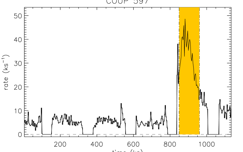
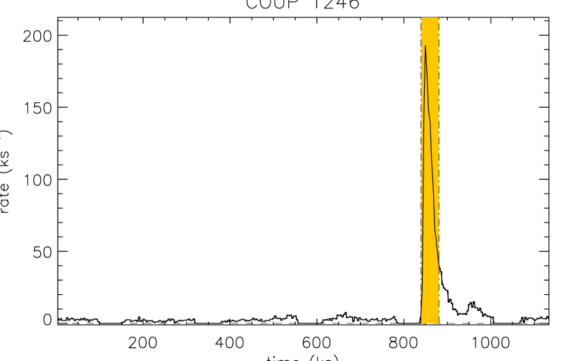
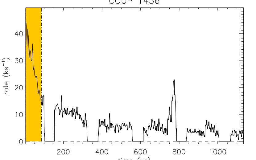
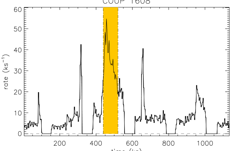
Figure 1: Observed light curves of the studied COUP sources. Time binning is 1 h. The shadowed area marks the time interval studied in this work.

4 Discussion of individual flares

From the sample of COUP sources showing large flares, we selected those sources studied by Favata et al. (2005) and Getman et al. (2008b) with the aim of comparing results. Each source was studied independently because the behavior of the flare is different in each star and, thus, the source and/or characteristics of the oscillations can differ. We focussed only on the light curves with significant oscillatory patterns. Figure 1 shows the light curve observed for each star during the COUP observations. Time binning is 1 h.

In the following, we present results for individual sources showing different behaviors. A summary of the results compared with those of Favata et al. (2005) and Getman et al. (2008a) is shown in Table 1. For completeness, we compare the results obtained assuming sausage-type oscillations (MHD scenario) with those of acoustic waves (HD scenario). Details on this comparison are given for each star.

4.1 COUP 332

The source COUP 332 (2MASS J05350934-0521415) underwent a long-duration flare ($>300$ ks) during the observations. Favata et al. (2005) derived a peak temperature $T_{\mathrm{peak}}=113$ MK and a very low electronic density $n_{e}=0.05\times 10^{10}$ cm^-3. Applying Reale et al. (1997), the authors determined a loop length $L\sim 7\times 10^{12}$ cm. This value is considerably higher than the one derived by Getman et al. (2008a), who obtained $L\sim 0.15-1.7\times 10^{12}$ cm. Aarnio et al. (2010) suggest a star-disk connection scenario in COUP 332, from the dust destruction radius estimated by them (see Table 1) and the loop length derived by Favata et al. (2005).

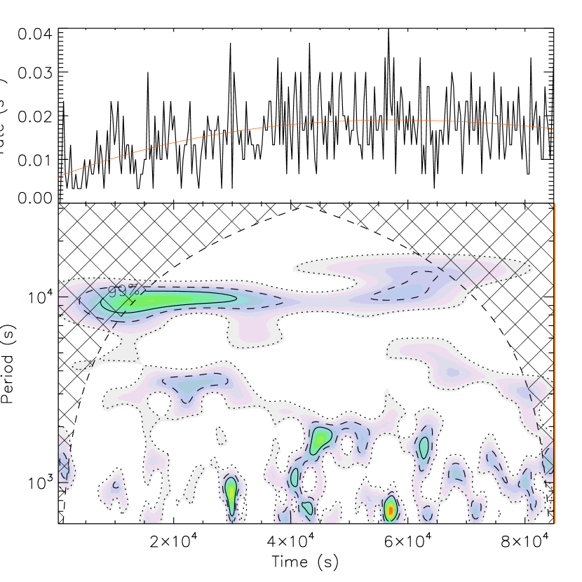
Figure 2: Wavelet power spectrum of a flare of source COUP 332 in the bottom panel. Contours are for confidence levels 67% (dotted line), 95% (dashed line) and 99% (continuous line). The hatched area is the cone of influence (COI), the region of the wavelet power spectrum in which edge effects become important (Torrence & Compo 1998). Top panel shows the observed light curve. Overplotted as a continuous line is the flare’s global shape. Time binning is 300 s.

The COUP observations are divided into periods of approximately 100 to 160 ks interrupted by 50 ks gaps. Together with the long duration of the flare of COUP 332, this fact causes a gap during the decay phase. We analyzed the first part of the flare, consisting on the rise phase and the first 50 ks of the decay, when the oscillation should be triggered. Figure 2 shows the result of the wavelet analysis. The top panel of the figure is the observed light curve, with a moving average overplotted as a continuous line. The bottom panel is the wavelet power spectrum after subtraction of the moving average to the observed light curve. The hatched area in the bottom panel is the cone of influence (COI), the region of the wavelet power spectrum in which edge effects become important (Torrence & Compo 1998). For our work, we analyze only features outside the COI.

A clear feature is detected during the rise phase ($P\sim 9$ ks) that evolves during more than 20 ks. The sound speed inside the tube, for an adiabatic plasma with $\gamma=5/3$, is $c_{s}=1.16\times 10^{4}\sqrt{T}=1.2\times 10^{8}$ cm s^-1. If we assume the oscillation with period $P=9\pm 1$ ks was caused by a wave moving along the tube at the velocity of the sound and this is the fundamental mode, the loop length would be $L=1.1\pm 0.1\times 10^{12}$ cm. This value is in the range given by Getman et al. (2008a) and lower than that given by Favata et al. (2005) who likely overestimated the loop length. We notice that Favata et al. (2005) did not determine uncertainties in the loop lengths and any comparison with our results should be made with caution.

Figure 3: Reconstructed light curve of COUP 332 for period $9\pm 1$ ks. The continuous lines are an exponential decay with e-folding time of $70$ ks. Time binning is 300 s.

From the light curve reconstruction at the period of the oscillation (see Fig. 3), the intensity of the perturbation is $\Delta I/I=0.17$. From Eq. 10, the magnetic field strength at the loop apex is $B_{\mathrm{min}}=24\pm 3$ G. This value is slightly higher than that given by pressure equilibrium ($B=12$ G; Favata et al. 2005). With an Alvén velocity $c_{a}\approx 2.18\times 10^{11}B/\sqrt{n}_{e}=2.4\times 10^{8}$ cm s^-1, the tube velocity for our plasma is $c_{t}=1.1\times 10^{8}$ cm s^-1. For an oscillation period $P=9\pm 1$ ks, the loop length becomes $L=0.98\pm 0.11\times 10^{12}$ cm, close to the length determined by assuming a wave moving at the velocity of the sound in the plasma.

Figure 3 also shows that the oscillation is damped. The quality factor of the oscillation is $Q\approx 20$ and the e-folding time is $t_{d}=60\pm 5$ ks. Comparing results with Ofman & Wang (2002), the damping of the oscillation does not seem to follow the scaling laws derived for thermal conduction dissipation in the Sun. The ratio $t_{d}/P=6.7\pm 1.9$ is within the range obtained from simulations by Selwa et al. (2005), where the authors considered only energy leakage into the photosphere as the wave damping mechanism.

4.2 COUP 597 (V2252 Ori)

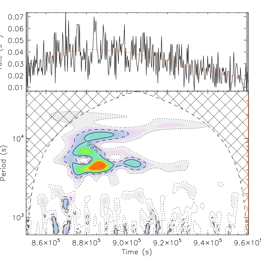
Figure 4: Wavelet power spectrum of a flare of source COUP 597 (V2252 Ori) in the bottom panel. Top panel shows the observed light curve in the time interval of the flare. Lines are as in Fig. 2. Time binning is 300 s.

Figure 4 shows the wavelet power spectrum of the flare detected during the COUP in V2252 Ori. The power spectrum of the subtracted light curve shows a significant feature extended between 4 and 12 ks. Its shape resembles somewhat that of Prox Cen during the flare underwent in 2009 (Srivastava et al. 2013). In that case, the authors identified two peaks in the power spectrum of the light curve and considered the longer period as the fundamental mode and the shorter period as the first harmonic. This scenario may be correct also for the flare observed in V2252 Ori. Figure 5 shows the reconstructed curve at periods $P\sim 4.5$ ks (dotted-dashed line) and $P\sim 10$ ks (continuos line). The amplitude of the $4.5$ ks feature is higher. According to Selwa et al. (2005), if we assume this feature is the first harmonic of the oscillation, the pulse of energy release should have occurred closer to the loop foot than to its apex.

Figure 5: Light curve reconstruction of COUP 597 (V2252 Ori) at periods $P=4.5$ ks (continuous line) and $P=10$ ks (dotted-dashed line). Time binning of 300 s.

With the plasma parameters determined by Favata et al. (2005, $T_{peak}=87$ MK and $n_{e}=5.2\times 10^{10}$ cm^-3), the sound velocity inside the flaring loop is $c_{s}=1.16\times 10^{4}\sqrt{T}=1.1\times 10^{8}$ cm s^-1 (assuming the plasma is adiabatic, with $\gamma=5/3$). If the oscillation was caused by an acoustic mode and we assume the 10 ks feature is the fundamental mode of the oscillation, $L=1.1\pm 0.2\times 10^{12}$ cm. If we consider the 4.5 ks is the fundamental mode, $L=4.9\pm 0.5\times 10^{11}$ cm. Both values of the loop length are close, but higher than that obtained by Favata et al. (2005). According to Aarnio et al. (2010), this flaring loop is possibly anchored to the inner protoplanetary disk (see Table 1).

As discussed in Section 3, for an optically thin plasma in static equilibrium, the magnetic field at the top of the loop can be determined if the amplitude of the oscillation is known (see Eq. 10). For our case, $\Delta I/I=0.3\pm 0.1$ and $B=162\pm 27$ G. This value is of the order of that determined from pressure equilibrium (Favata et al. 2005). The Alfvén velocity inside the loop is $c_{a}=\approx 2.18\times 10^{11}B/\sqrt{n}_{e}=1.55\times 10^{8}$ cm s^-1 and the tube velocity (the minimum velocity of the slow mode), $c_{t}=8.97\times 10^{7}$ cm s^-1. For this velocity, $L=4.0\pm 0.5\times 10^{11}$ cm assuming the 4.5 ks feature is the actual fundamental mode, $L=9.0\pm 0.9\times 10^{11}$ cm if we use the 10 ks (similar to the value derived assuming acoustic waves).

The two oscillations detected are not very efficiently damped ($Q\approx 25$; see Figure 5). Contrarily to COUP 332, the damping time of these oscillations $\tau_{d}\sim 45\leavevmode\nobreak\ ks$ do follow the scaling law of Ofman & Wang (2002) for low temperature plasma ($T\sim 6$ MK). Those laws were obtained for wave dissipation by thermal conduction.

4.3 COUP 1246 (V1530 Ori)

V1530 Ori was included in Category 3 (“the inner edge of the dust disk is clearly beyond reach of the magnetic flaring loop”) by Aarnio et al. (2010). Consequently, the flaring loop cannot be anchored to the accretion disk. Favata et al. (2005) determined a loop length $L=4.0\times 10^{11}$ cm ($L/R_{\star}=3.4$) and a magnetic field strength $B=240$ G. The value for the loop length determined by Getman et al. (2008a) is slightly smaller ($L\sim 2.4\times 10^{11}$ cm) but still the loop is long ($L/R_{\star}\sim 2$).

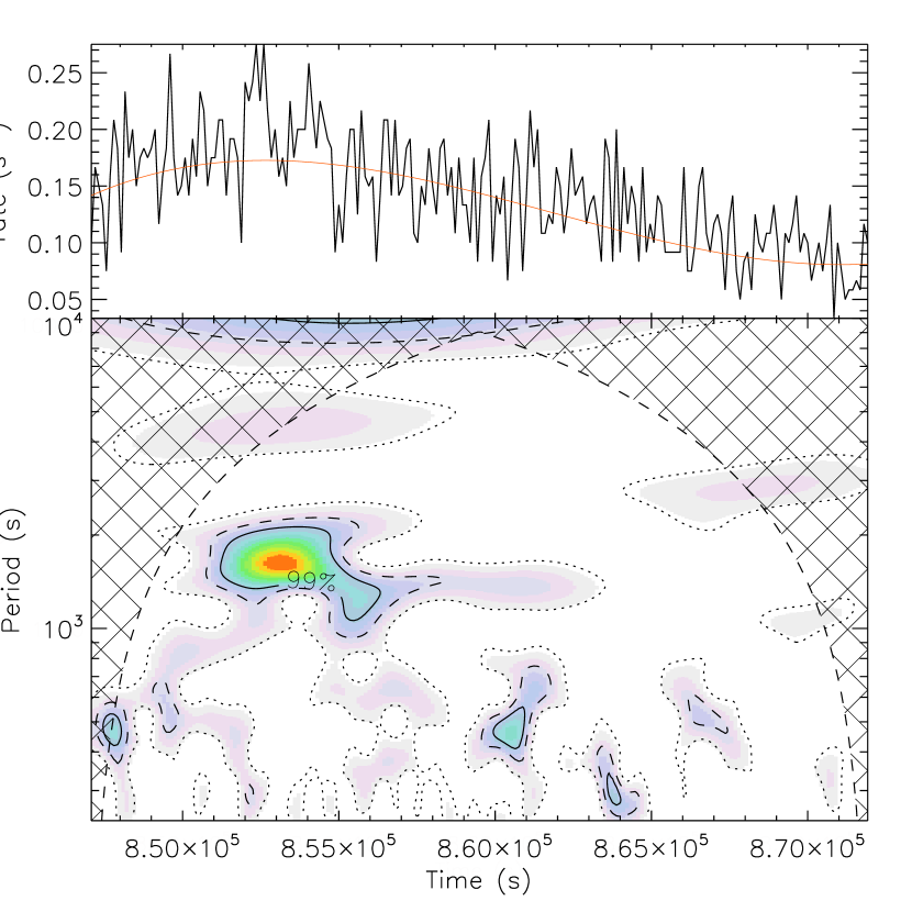
Figure 6: Wavelet power spectrum of the source COUP 1246 (V1530 Ori). Time binning is 120 s. Panels and lines are as in Figure 4.

The wavelet power spectrum of the flare observed in V1530 Ori (Figure 6) shows a feature outside the cone of influence. Thus, we do not analyze it here. The feature at $P\approx 1.8$ ks is detected during the rise phase, close to the flare maximum. From the peak temperature $T=270$ MK determined by Favata et al. (2005), the sound speed of the plasma inside the magnetic tube is $c_{s}=1.9\times 10^{8}$ cm s^-1. An acoustic wave would travel $3.4\times 10^{11}$ cm in 1.8 ks. This value is close to the loop length determined by Favata et al. (2005).

Figure 7: Reconstructed light curve of COUP 1246 (V1530 Ori) for periods $1.0-2.0$ ks. Time binning is 120 s. Continuous line is a exponential decay with e-folding time of 8.5 ks (dashed line is for e-folding time of 7.5 ks).

The reconstructed light curve for the period range $1.0\leavevmode\nobreak\ \mathrm{ks}<P<2.0$ ks is shown in Figure 7. The e-folding time of the oscillation is $8.5\pm 1.0$ ks. This value does not follow the scaling laws for damping in solar flares treated in Ofman & Wang (2002) and Mariska (2005). In those works, damping was driven by thermal conduction processes. The long decay time obtained in this oscillation suggests the damping in this flare was not caused by thermal conduction but by leakage into the photosphere (see Selwa et al. 2005).

The intensity of the oscillation is $\Delta I/I=0.2\pm 0.04$. From Eq. 10, the magnetic field strength at the loop apex is $B_{\mathrm{min}}=362\pm 45$ G, considerably higher than the value derived from pressure equilibrium ($B=240$ G; Favata et al. 2005). With this magnetic field, the Alfvén velocity inside the tube is $c_{A}=3.3\times 10^{8}$ cm s^-1 (assuming $n_{e}=5.6\times 10^{10}$ cm^-3; Favata et al. 2005), for a tube velocity $c_{t}=1.7\times 10^{8}$ cm s^-1. Using a period $P=1.8\pm 0.2$ ks for the fundamental mode of oscillations, we derive a length loop $L=3.4\pm 0.4\times 10^{11}$ cm, as for the case of an acoustic wave.

4.4 COUP 1456

During the COUP observations, this source showed a continuous decrease in its count rate during more than 500 ks, likely produced by the decay of a large flaring event. This flare was not studied by Favata et al. (2005) or Getman et al. (2008a), most likely because the flare maximum took place before the observation started. In the wavelet power spectrum of the first 90 ks of the observation (Figure 8) the source shows a double peak feature at $\sim 6$ ks. Before it, a peak at $\sim 3.0$ ks is detected. The peak at the highest frequency may be related to the first harmonic of the oscillation and the feature with the longest period to the fundamental mode. The detection of the first harmonic before the detection of the fundamental mode can be related to the location of the initial pulse (energy input) in the loop (Selwa et al. 2005). The first harmonic is excited when the initial pulse is launched close to the top of the loop. This harmonic is more sensitive to the inhomogeneities of the medium and, hence, it is more efficiently damped. On contrast, the fundamental wave tends to occupy the entire loop over its length and it is damped less efficiently.

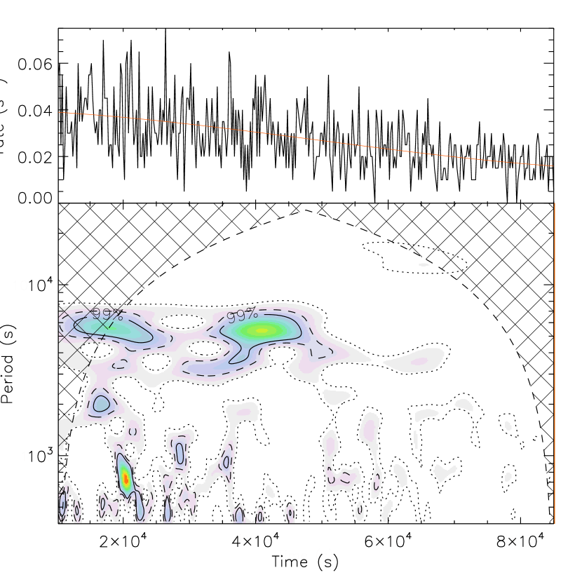
Figure 8: Light curve and wavelet power spectrum of the source COUP 1456. Time binning is 200 s. Lines are as in Figure 2.

We may assume the temperature at the beginning of the decay phase is $T=20-40$ MK taking the results of Getman et al. (2008a) for other sources into account. For a 20 MK plasma, the sound velocity in the medium is $c_{s}=7.4\times 10^{7}$ cm s^-1. For the fundamental wave ($P=6\pm 0.5$ ks) moving at the sound velocity, $L=4.4\pm 0.4\times 10^{11}$ cm, similar to other loop lengths determined in previous sections for other flaring loops.

4.5 COUP 1608 (OW Ori)

Getman et al. (2008b) concluded that OW Ori is the only star in the COUP sample where the flare took place in a loop connecting the star with the disk. Actually, the authors assumed that the disk of the stars in their sample were all truncated at the stellar co-rotation radius. Aarnio et al. (2010) showed that this assumption is wrong in some cases. Nevertheless, OW Ori remains the most promising case to show a flare in a star-disk connected magnetic tube because the length derived in the literature by distinct authors is always above the co-rotation radius (see Table 1). Getman et al. (2008a) determined a loop length of $\sim 8\times 10^{11}$ cm, similar to the value determined by Favata et al. (2005). This length corresponds to 6.7 R_⋆, which is longer than the co-rotation radius. This result strongly suggests the energy release occurred in a magnetic tube connecting the star with the accretion disk.

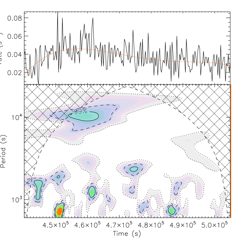
Figure 9: Wavelet power spectrum of the source COUP 1608 (OW Ori). Lines and panels are as in Figure 2. Time binning is 300 s.

Figure 9 shows the wavelet power spectrum of the flare light curve of OW Ori in the COUP. The global shape of the flare was subtracted from the light curve by smoothing the observed curve with a moving average. The feature at $P\approx 10$ ks is clearly identified. It starts just before the flare maximum. According to the parameters determined in Favata et al. (2005) for this flare, $n_{e}=10^{10}$ cm^-3 and $T_{peak}=258$ MK. The sound velocity inside the tube is, then, $c_{s}=1.8\times 10^{8}$ cm s^-1. Assuming the feature at $P=10$ ks is the fundamental mode of an oscillation propagating along the magnetic tube, $L=1.8\pm 0.2\times 10^{12}$ cm.

Favata et al. (2005) determined a magnetic field strength $B=96$ G assuming pressure equilibrium. From Eq. 10, $B=299\pm 2$ G ($\Delta I/I=0.05$ for this flare). This value is quite higher than that determined by Favata et al. (2005). Thus, then Alfvén velocity inside the tube is $c_{a}=6.5\times 10^{8}$ cm s^-1 and the tube velocity $c_{t}=1.8\times 10^{8}$ cm s^-1. With this velocity, $L=1.8\pm 0.2\times 10^{12}$ cm, as for the sonic wave. This length is compatible with the star-disk connection scenario.

Table 1: Parameters of the flares.

Favata et al. (2005)

Getman et al. (2008a)

This work

Src.

$T_{\mathrm{peak}}$

$n_{\mathrm{e}}$

$B^{\mathrm{a}}$

$L$

$L$

$R_{\mathrm{cor}}$

$R_{\mathrm{dust}}^{\mathrm{b}}$

$L_{\mathrm{HD}}$

$L_{\mathrm{MHD}}$

$B_{\mathrm{min}}$

star-disk

(MK)

($10^{10}$ cm)

(G)

($10^{12}$ cm)

($10^{12}$ cm)

($10^{12}$ cm)

($10^{12}$ cm)

($10^{12}$ cm)

($10^{12}$ cm)

(G)

connection

332

113

0.04

12

7.3

$0.5-1.7$

…

0.56

$1.1\pm 0.1$

$0.98\pm 0.11$

$24\pm 3$

Y

597

87

5.40

128

$0-0.75$

$0.08-0.47$

…

1.99

$1.1\pm 0.2$

$0.90\pm 0.09$

$162\pm 27$

Y?

1246

270

5.60

240

$0.32-0.47$

0.24

0.54

0.48

$0.34\pm 0.04$

$0.34\pm 0.08$

$365\pm 45$

N

1456

40

…

…

…

…

…

…

$0.44\pm 0.04$

…

…

N?

1608

258

1.00

96

$0-0.99$

$0.74-0.77$

0.60

0.75

$1.8\pm 0.2$

$1.8\pm 0.2$

$299\pm 2$

Y

5 Summary and Conclusions

We applied wavelet analysis tools to reveal oscillation patterns in the flare light curves of T Tauri stars observed by the COUP. With the results obtained from this analysis and the plasma characteristics previously determined, we inferred the length of the flaring loops. Our analysis is restricted to those flares showing a significant oscillation. Other flares were also studied but their analysis gave uncertain results and they were not included here. The limitations of our results are linked only to the uncertainties in the plasma parameters taken from the literature. In particular, the plasma temperatures in Favata et al. (2005) are not well constrained in some cases. We interpret oscillations as caused by the fundamental mode and/or the first harmonic inside the loop. Higher order harmonics require higher energies to be released (e.g. Selwa et al. 2005).

In our study, we did not assume the observed flares occurs in a single loop a priori. The wavelet analysis was applied to the light curves of flaring CTTS of the COUP. When an oscillation pattern was revealed, we determined plasma properties including the length of the oscillating structure. This value depends only on the oscillation period and on the wave velocity. In the very unlikely case of more than one loop oscillating in coherence (see Section 1), all of them would oscillate at the same frequency and the result would be applicable to each loop.

Assuming a simple physical model for triggering of an oscillation in a magnetic tube, other characteristics of the coronal medium can be inferred. In this work, we determined magnetic field strengths at the loop apex. Our results show that flares may take place in magnetic tubes connecting the star with its accretion disk. In particular, we find that at least three stars (COUP 332, COUP 597 –  or V2252 Ori – and COUP 1608 – or OW Ori –) have magnetic tubes potentially connecting the star with its accretion disk. According to MHD simulations by Orlando et al. (2011), a flare in a magnetic tube connecting the star with the disk may trigger subsequent accretion by the star, in time scales of hours to days after the flare took place. In such a case, UV enhance should be detected in these stars after some hour after the flare maximum. A simultaneous long X-ray and UV observation of these stellar systems would eventually confirm this scenario.

We conclude that analyzing oscillations in flare light curves is a powerful tool to investigate the actual extension of the corona of stars and determine other parameters. The particularly case of classical T Tauri stars is a good check point.

References

- Aarnio et al. (2010) Aarnio, A. N., Stassun, K. G., & Matt, S. P. 2010, ApJ, 717, 93
- Aschwanden et al. (1999) Aschwanden, M. J., Fetcher, L., Schrijver, C. J., & Alexander, D. 1999, ApJ, 520, 880
- Banerjee et al. (2000) Banerjee, D., O’Shea, E., & Doyle, J. G. 2000, Sol. Phys., 196, 63
- Camenzind (1990) Camenzind, M. 1990, Reviews in Modern Astronomy, 3, 234
- De Moortel et al. (2002) De Moortel, I., Hood, A. W., & Ireland, J. 2002, A&A, 381, 311
- Favata et al. (2005) Favata, F., Flaccomio, E., Reale, F., et al. 2005, ApJS, 160, 469
- Ge (2007) Ge, Z. 2007, Annales Geophysicae, 25, 2259
- Getman et al. (2005) Getman, K. V., Flaccomio, E., Broos, P. S., et al. 2005, ApJS, 160, 319
- Getman et al. (2008a) Getman, K. V., Feigelson, E. D., Broos, P., Micela, G., & Garmire, G. P., 2008a, ApJ, 688, 418
- Getman et al. (2008b) Getman, K. V., Feigelson, E. D., Micela, G., et al. 2008b, ApJ, 688, 437
- Ghosh & Lamb (1978) Ghosh, P., & Lamb, F. K. 1978, ApJ, 223, L83
- Gómez de Castro et al. (2013) Gómez de Castro, A. I., López-Santiago, J., & Talavera, A. 2013, MNRAS, 429, L1
- Goodson et al. (1997) Goodson, A. P., Winglee, R. M., Böhm, K.-H. 1997, ApJ, 489, 199
- Güdel (2004) Güdel, M. 2004, A&ARv, 12, 71
- Hartman (1989) Hartmann, L. 1998, Accretion Processes in Star Formation, Cambridge: Cambridge Univ. Press
- Jess et al. (2012) Jess, D. B., De Moortel, I., Mathioudakis, M., et al. 2012, ApJ, 757, 160
- Kim et al. (2012) Kim, S., Nakariakov, V. M., & Shibasaki, K. 2012, ApJ, 756, L36
- Koenigl (1991) Koenigl, A. 1991, ApJ, 370, L39
- Kopylova et al. (2002) Kopylova, Y. G., Stepanov, A. V., & Tsap, Y. T. 2002, Astronomy Letters, 28, 783
- Liu & Ofman (2014) Liu, W., & Ofman, L. 2014, Sol. Phys., 289, 3233
- López-Santiago et al. (2010) López-Santiago, J., Crespo-Chacón, I., Micela, G., & Reale, F. 2010, ApJ, 712, 78
- Lovelace et al. (1995) Lovelace, R. V. E., Romanova, M. M., & Bisnovatyi-Kogan, G. S. 1995, MNRAS, 275, 244
- Mariska (2005) Mariska, J. T. 2005, ApJ, 620, L67
- Mathioudakis et al. (2003) Mathioudakis, M., Seiradakis, J. H., Williams, D. R., et al. 2003, A&A, 403, 1101
- Mathioudakis et al. (2006) Mathioudakis, M., Bloomfield, D. S., Jess, D. B., Dhillon, V. S., & Marsh, T. R. 2006, A&A, 456, 323
- Mitra-Kraev et al. (2005) Mitra-Kraev, U., Harra, L. K., Williams, D. R., & Kraev, E. 2005, A&A, 436, 1041
- Nakariakov et al. (1999) Nakariakov, V. M., Ofman, L., Deluca, E. E., Roberts, B., & Davila, J. M. 1999, Science, 285, 862
- Nakariakov & Ofman (2001) Nakariakov, V. M., & Ofman, L. 2001, A&A, 372, L53
- Nakariakov & Melnikov (2009) Nakariakov, V. M., & Melnikov, V. F., 2009, Space Sci. Rev., 149, 119
- Ofman et al. (2000) Ofman, L., Romoli, M., Poletto, G., Noci, G., & Kohl, J. L. 2000, ApJ, 529, 592
- Ofman & Wang (2002) Ofman, L., & Wang, T. 2002, ApJ, 580, L85
- Ofman & Sui (2006) Ofman, L., & Sui, L. 2006, ApJ, 644, L149
- Orlando et al. (2011) Orlando, S., Reale, F., Peres, G., & Mignone, A. 2011, MNRAS, 415, 3380
- Pandey & Srivastava (2009) Pandey, J. C., & Srivastava, A. K. 2009, ApJ, 697, L153
- Pillitteri et al. (2014) Pillitteri, I., Wolk, S. J., Lopez-Santiago, J., et al. 2014, ApJ, 785, 145
- Prisinzano et al. (2008) Prisinzano, L., Micela, G., Flaccomio, E., et al. 2008, ApJ, 677, 401
- Reale et al. (1997) Reale, F., Betta, R., Peres, G., Serio, S., & McTiernan, J. 1997, A&A, 325, 782
- Reale (2007) Reale, F. 2007, A&A, 471, 271
- Roberts et al. (1984) Roberts, B., Edwin, P. M., & Benz, A. O. 1984, ApJ, 279, 857
- Selwa et al. (2005) Selwa, M., Murawski, K., & Solanki, K. 2005, A&A, 436, 701
- Serio et al. (1991) Serio, S., Reale, F., Jakimiec, J., Sylwester, B., & Sylwester, J. 1991, A&A, 241, 197
- Srivastava et al. (2008) Srivastava, A. K., Zaqarashvili, T. V., Uddin, W., Dwivedi, B. N., & Kumar, P. 2008, MNRAS, 388, 1899
- Srivastava et al. (2013) Srivastava, A. K., Lalitha, S., & Pandey, J. C. 2013, ApJ, 778, L28
- Stepanov et al. (2012) Stepanov, A. V., Zaitsev, V. V., & Nakariakov, V. M. 2012, Stellar Coronal Seismology as a Diagnostic Tool for Flare Plasma, by A.V. Stepanov, V.V. Zaitsev and V.M. Nakariakov. Wiley-VCH Verlag GmbH & Co. KGaA, Weinheim, Germany, 2012
- Torrence & Compo (1998) Torrence, C., & Compo, G. P. 1998, Bull. Amer. Meteor. Soc., 79, 61
- Verwichte et al. (2004) Verwichte, E., Nakariakov, V. M., Ofman, L., & Deluca, E. E. 2004, Sol. Phys., 223, 77
- Verwichte et al. (2009) Verwichte, E., Aschwanden, M. J., Van Doorsselaere, T., Foullon, C., & Nakariakov, V. M. 2009, ApJ, 698, 397
- Welsh et al. (2006) Welsh, B. Y., Whetley, J., Browne, S., E., et al., 2006, A&A, 458, 921
- Zaitsev & Stepanov (1989) Zaitsev, V. V., & Stepanov, A. V. 1989, Sov. Astron. Lett., 15, 66