How to assess case-finding in chronic diseases: Comparison of different indices.

Abstract

Recently, we have proposed a new illness-death model that comprises a state of undiagnosed chronic disease preceding the diagnosed disease. Based on this model, the question arises how case-finding can be assessed in the presence of mortality from all these states. We simulate two scenarios of different performance of case-finding and apply several indices to assess case-finding in both scenarios. One of the prevalence based indices leads to wrong conclusions. Some indices are partly insensitive to distinguish the quality of case-finding. The incidence based indices perform well. If possible, incidence based indices should be preferred.

Keywords: Case-finding; Screening; Chronic diseases; Incidence; Prevalence; Mortality; Compartment model; Partial differential equation.

1 Introduction

Many chronic diseases have a preclinical phase, when the disease is principally detectable but has not been diagnosed yet. Examples are cardiovascular disease, diabetes, chronic obstructive pulmonary disease, depression, or dementia.

We call all collective activities and efforts, in which cases of a specific chronic disease not known to the health services are searched for, case-finding. Case-finding in this sense is a very broad term, which comprises screening, application of diagnostic tests and all other activities and policies of detecting cases of a chronic disease. Efforts in case-finding vary substantially, both globally and temporally. Geographical variations are due to different health systems, available resources and differences in the risk for certain diseases in a region or country. For example, efforts in case-finding for dementia are likely to be higher in older populations, e.g., in the industrialised countries. Reasons for temporal changes in case-finding of chronic diseases are manifold as well. Besides technical progress in making diagnostic tests cheaper and more practicable, varying awareness of patients and physicians may lead to an earlier or later diagnosis of the disease.

Early detection of diseases might be important for two reasons. First, in many cases it is favourable if the disease is treated early to make effective treatment possible, e.g. cancer [1], diabetes [2], or chronic kidney disease [3]. Second, patients with an undiagnosed disease already have an elevated risk for unfavourable outcomes. For example, persons with undiagnosed diabetes have an about 50% increased risk of all-cause mortality compared to a healthy person [4, Table 2]. Another example is undiagnosed chronic obstructive pulmonary disease, which is rather frequent [5] and associated with a severe loss of quality of life [6].

Given the enormous importance of case-finding in chronic diseases, we want to examine different measures of how to quantitatively assess the activities of case-finding of a specific chronic disease. The question arises what epidemiological measures are suitable for describing the performance of case-finding on the population level.

We give an example from the epidemiology of diabetes. Table 1 shows the prevalence undiagnosed and diagnosed diabetes for men and women in two age groups of the KORA study [7]. In men, we see that with increasing age the percentages of undiagnosed and diagnosed diabetes increase. The situation is different in women. As the age increases, the prevalence of undiagnosed and diagnosed diabetes rises and lowers, respectively. The key question of this article is: which situation is more desirable with respect to case-finding, the situation of men or the one of women?

Table 1: Sex-specific prevalence of undiagnosed and diagnosed diabetes in two age-groups of the KORA study [7].

Age	Undiagnosed diabetes (in %)		Diagnosed diabetes (in %)
(years)	Men	Women	Men	Women
60–64	8.1	7.3	7.2	9.7
65–69	8.9	8.2	13.3	8.2

Before we try to answer this question, we describe the underlying epidemiological model for assessing the performance of case-finding.

2 Epidemiological model

If we are interested in evaluating the efforts of case-finding in a population, we consider each person being exactly in one of the depicted states shown in Figure 1: Normal, i.e., healthy with respect to the considered chronic disease, Undiagnosed, Diagnosed or Dead. At the birth each person is in the Normal state (here we just consider diseases acquired after birth). During the life course, the person may contract the disease and enters the Undiagnosed state. In a screening program, or as the disease becomes symptomatic, or during some routine medical examinations, the disease may be diagnosed and the person enters the Diagnosed state. Persons may decease from any of these three states. Note that we are just considering chronic diseases. Hence, backward steps from the Undiagnosed state to the Normal state are not possible. Similarly, we assume that once a person has got a diagnosis the disease remains detected for ever. Thus, we assume that there is no loss of such information.

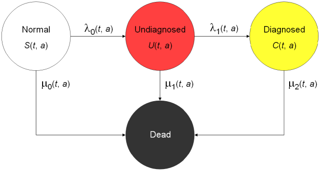
Figure 1: Chronic disease model. Persons in the state Normal are healthy with respect to the disease under consideration. After onset of the disease, they change to state Undiagnosed and later to the state Diagnosed. The absorbing state Dead can be reached from all other states. The percentages of persons in the states and the transition rates depend on calendar time $t$ and age $a.$

In [8] we described relations between the transition rates $\lambda_{\ell}(t,a),~{}\ell=0,1,$ and $\mu_{k}(t,a),~{}k=0,1,2$, in the model and the percentages of persons in the states. As in [8] let $p_{k}(t,a)$ denote the fraction of persons aged $a$ at time $t$ in state $k,~{}k=0,1,2.$ For example, $p_{1}(t,a)$ is the fraction of persons in the population who are aged $a$ at time $t$ and are in the Undiagnosed state ($k=1$).

3 Assessment of case-finding

In this section, we describe measures for assessing the performance of case-finding. We distinguish figures based on the prevalences and figures based on the transition rates between the states in the epidemiological model (cf. Figure 1).

3.1 Figures based on the prevalence

The first figure to approach case-finding, is the proportion of detected cases from the total cases [9], i.e.,

$$\wp_{1}=\tfrac{p_{2}}{p_{1}+p_{2}}.$$ (1)

Similar to the dark figure in criminology, the reciprocal of $\wp_{1}$ describes the factor the diagnosed cases have to be multiplied with to obtain the number of all cases of the chronic disease. Obviously, it holds $0\leq\wp_{1}\leq 1.$ A high value in $\wp_{1}$ is usually interpreted as advantageous [9].

Analogously, it may be useful to consider the ratio

$$\wp_{2}=\tfrac{p_{1}}{p_{0}+p_{1}}.$$ (2)

This ratio relates the number of persons in the undiagnosed state to all persons who do not have a diagnosis, i.e., the healthy and the undiagnosed. The idea behind the measure $\wp_{2}$ is that case-finding can be thought of distinguishing persons from a pool consisting of healthy and undiagnosed persons. This pool of healthy and undiagnosed persons may be seen as the search space. The search space is subject to the activities of case-finding. Once an undiagnosed person is undoubtedly identified as a case, this person gets a diagnosis and is removed from the search space henceforth. As the disease under consideration is chronic, there is no way back into the search space. In contrast to $\wp_{1}$, the figure $\wp_{2}$ just refers to the persons who are at risk for a possible diagnosis. The fraction of persons with a diagnosis does not play a role.

Again, it holds $0\leq\wp_{2}\leq 1.$ Ideally, $\wp_{2}$ is 0, i.e., all undetected cases are removed from the search space. The closer $\wp_{2}$ approaches 1, the more the search space is dominated by the undiagnosed persons. Thus, a lower value of $\wp_{2}$ is advantageous in assessing case-finding.

If we calculate the measures $\wp_{1}$ and $\wp_{2}$ for the data in Table 1, we obtain the values shown in Table 2.

Table 2: Age- and sex-specific ratios $\wp_{1}$ and $\wp_{2}$ for the data in Table 1.

Age	$\wp_{1}$ (in %)		$\wp_{2}$ (in %)
(years)	Men	Women	Men	Women
60–64	47	57	9	8
65–69	60	50	10	9

For men, the measure $\wp_{1}$ increases from 47% to 60% as the age increases. Thus, $\wp_{1}$ indicates that with increasing age the performance of case-finding improves. However, $\wp_{2}$ indicates that the performance of case-finding in men deteriorates from the lower age class to the higher. Thus, the measures $\wp_{1}$ and $\wp_{2}$ yield contradicting findings in assessing the performance of case-finding.

As the age increases, the measure $\wp_{1}$ for women decreases from 57% to 50%, which indicates a worsening of case-finding. Similarly, $\wp_{2}$ shows a worsening. In women, the figures $\wp_{1}$ and $\wp_{2}$ allow the same conclusion. This example from the KORA study shows that at least one of the figures $\wp_{1}$ or $\wp_{2}$ is not suitable for assessing the performance of case-finding. We will come back later to this point.

3.2 Figures based on the transition rates

Apart from the figures based on the prevalences, we may consider figures based on the transitions in the model.

3.2.1 Incidence rate ratio

In [8] we used the rate ratio $\operatorname{DR}=\tfrac{\lambda_{1}}{\lambda_{0}},$ which relates the instantaneous risk (hazard) of transiting to the diagnosed state to the risk of becoming an undetected case. As it is unlikely to be diagnosed immediately after entering the undiagnosed state, we introduce a delay parameter $\gamma,~{}\gamma\geq 0,$ and define

$$\operatorname{DR}_{\gamma}(t,a)=\frac{\lambda_{1}(t+\gamma,a+\gamma)}{\lambda_{0}(t,a)}.$$

Obviously, it holds $\operatorname{DR}=\operatorname{DR}_{0}.$

3.2.2 Deaths without a diagnosis

An important figure is the fraction of healthy persons aged $a$ at time $t$ who become incident undiagnosed cases at time $t$ and die within $\gamma>0$ time units without a diagnosis. As these persons do not have a diagnosis, they never were treated. To develop this figure we first calculate the probability of dying $P^{(\text{dead})}_{\gamma}$ during the first $\gamma>0$ time units in the undiagnosed state:

$$P^{(\text{dead})}_{\gamma}(t,a)=\int_{0}^{\gamma}\mu_{1}(t+s,a+s)\,\exp\Bigl{(}-\int_{0}^{s}(\lambda_{1}+\mu_{1})(t+\tau,a+\tau)\mathrm{d}\tau\Bigr{)}\,\mathrm{d}s.$$ (3)

Then, the probability $P^{(\text{dead})}_{\gamma}$ is combined with the incidence rate $\lambda_{0}:$

$$\Phi_{\gamma}(t,a)=\lambda_{0}(t,a)\,P^{(\text{dead})}_{\gamma}(t,a).$$ (4)

Then, $\Phi_{\gamma}(t,a)$ is the number of death cases per one healthy person aged $a$ at time $t$, who becomes an incident undiagnosed case at $t$ and dies within $\gamma$ time units without diagnosis. To get an integer number, one may multiply with a power of 10, say, 100,000. These originally 100,000 healthy persons never had the chance of obtaining a treatment.

3.3 Other figures

In the field of infectious disease epidemiology, sometimes the case detection rate ($\operatorname{CDR}$) is considered. The CDR is the notification rate of incident cases over the total incidence rate. Roughly speaking, it is the proportion of detected incident cases from the total incident cases [10]. In our terminology, the $\operatorname{CDR}$ can be calculated as:

$$\operatorname{CDR}=\operatorname{DR}_{0}\,\wp_{2}.$$ (5)

A proof for this relation can be found in the appendix.

4 Simulation study

In the introducing example from the KORA study, we have seen that the prevalence-based measures $\wp_{1}$ and $\wp_{2}$ have come to contradicting conclusions about the performance of case-finding in the male population. So far, it remains open which measure is more appropriate for the assessment of case-finding.

In this section, we conduct a simulation study with two different settings to answer this question. In one setting, the underlying (true) performance of case-finding worsens over time, whereas in the other setting the true performance betters. For both settings, we calculate the introduced measures of assessing the case-finding by comparing two points in time. For setting up the simulation, we use a system of partial differential equations with known transition rates.

4.1 Partial differential equations

Based on the epidemiological model in Figure 1, we have shown that in a population without migration and with sufficiently smooth transition rates $\lambda_{\ell},~{}\ell=0,1,~{}\mu_{k},k=0,1,2,$ the prevalences $p_{k},~{}k=0,1,2,$ are governed by a set of partial differential equations [8]:

$$(\partial_{t}+\partial_{a})p_{1} =\lambda_{0}-\bigl{(}\lambda_{0}+\lambda_{1}+\mu_{1}-\mu_{0}\bigr{)}\,p_{1}-\lambda_{0}\,p_{2}+\lambda_{0}$$ (6)

$$(\partial_{t}+\partial_{a})p_{2} =\lambda_{1}\,p_{1}-\bigl{(}\mu_{2}-\mu\bigr{)}\,p_{2}.$$ (7)

The notation $\partial_{x}$ means the partial derivative with respect to $x,~{}x\in\{t,a\}$. In Equations (6) – (7), the term $\mu$ is the overall mortality (general mortality), which can be written as

$$\mu=p_{0}\,\mu_{0}+p_{1}\,\mu_{1}+p_{2}\,\mu_{2}.$$ (8)

The prevalence $p_{0}$ can be calculated by using the equation $p_{0}=1-p_{1}-p_{2}.$ Thus, together with the initial conditions $p_{1}(t,0)=p_{2}(t,0)=0$ for all $t,$ the system (6) – (7) completely describes the dynamics of the disease in the considered population.

For later use, we remark that Equations (6) – (7) can be transformed into following system:

$$(\partial_{t}+\partial_{a})p_{1} =\lambda_{0}\,(1-p_{2})-(\lambda_{0}+\lambda_{1}+\mu_{1}-\mu_{0})\,p_{1}+p_{1}\,z$$ (9)

$$(\partial_{t}+\partial_{a})p_{2} =-(\mu_{2}-\mu_{0})\,p_{2}+\lambda_{1}\,p_{1}+p_{2}\,z,$$ (10)

where $z=p_{1}\,(\mu_{1}-\mu_{0})+p_{2}\,(\mu_{2}-\mu_{0}).$

We will integrate the system (9) – (10) using the Method of Characteristics [11] and Runge-Kutta integration [12]. All calculations are done with the software R (The R Foundation of Statistical Computing).

4.1.1 Transition rates between the states

The incidence rate $\lambda_{0}$ is chosen to be

$$\lambda_{0}(t,a)=\frac{1}{3}\times 10^{-4}\times(a-30)_{+}\times 1.015^{t},$$ (11)

which in magnitude coarsely mimics the incidence of type 2 diabetes in males [13].

The rate $\lambda_{1}$ is assumed to be a sigmoid function with a steep increase between the 20th and 50th year of age:

$$\lambda_{1}(t,a,\varepsilon)=\frac{0.02}{1+\exp\bigl{(}-0.25\times(a-35)\bigr{)}}\times\bigl{(}1.015+\varepsilon\bigr{)}^{t}.$$ (12)

This rate mimics an hypothetical awareness for type 2 diabetes, which is assumed to increase after an onset at $a=20.$

From Eq. (11), we observe that the rate $\lambda_{0}$ rises with calendar time $t$. For the rate $\lambda_{1}$ we choose two simulation settings (A) and (B) with $\varepsilon_{A}=-0.016$ and $\varepsilon_{B}=0.01.$ In settings A and B, the annual change $(1.015+\varepsilon)$ of $\lambda_{1}$ is negative and positive, respectively. This will lead to an accumulation of undetected cases over calendar time in setting A and a slowly decreasing reservoir of undetected cases in setting B.

Figure 2 shows the age courses of $\lambda_{0}$ and $\lambda_{1}$ for $t=0.$ Note that for $t=0$ the rates $\lambda_{1}$ in setting A and B are the same:

$$\lambda_{1}(0,a,\varepsilon_{A})=\lambda_{1}(0,a,\varepsilon_{B}),~{}\text{for all }a.$$

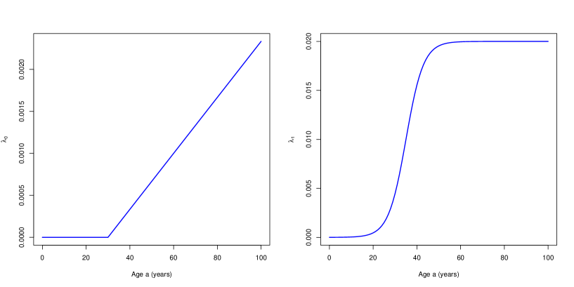
Figure 2: Age courses of $\lambda_{0}$ (left) and $\lambda_{1}$ (right) in year $t=0.$

We choose Gompertz mortality rates, [14, Eq. (9.1)]:

$$\mu_{k}(t,a)=\exp(-\xi_{k}+\eta_{k}\,a)\times(1-\rho_{k})^{t},~{}k=0,1,2,$$ (13)

with the coefficients as in Table 3. The mortality rates of many populations approximately follow a Gompertz law, and the numbers roughly reflect the mortality of German males in the past century. Calendar time $t$ in this sense is the time (in years) after 1900.

For further references and a critical discussion of the Gompertz law of mortality see, for instance, [15]. The yearly decrements $\rho_{k}$ are chosen with a view to trends in mortality. The choice $\rho_{2}>\rho_{1}$ is motivated by the fact that medical progress is reaching treated persons more than untreated.

Table 3: Coefficients of the Gompertz mortality rates $\mu_{k},~{}k=0,1,2$.

$k$	$\xi_{k}$	$\eta_{k}$	$\rho_{k}$
$0$	9.8	0.09	0.015
$1$	9.7	0.10	0.015
$2$	9.2	0.11	0.030

4.1.2 Prevalence

Integrating Eq. (9) – (10) with the rates given in Eq. (11) – (12) and the Gompertz mortalities (Eq. (13) and Table 3), we obtain $p_{1}$ and $p_{2}$ for the years $t=100$ and $t=110$ in both simulations as shown in Table 4.

Table 4: Age-specific prevalence of undiagnosed ($p_{1}$) and diagnosed ($p_{2}$) disease in the simulation.

Age	Setting A				Setting B
(years)	$p_{1}$ (in %)		$p_{2}$ (in %)		$p_{1}$ (in %)		$p_{2}$ (in %)
	$t=100$	$t=110$	$t=100$	$t=110$	$t=100$	$t=110$	$t=100$	$t=110$
45	1.4	1.7	0.10	0.12	0.74	0.73	0.79	1.0
60	4.7	5.5	0.81	0.94	1.6	1.5	4.0	5.0
75	8.4	9.8	2.2	2.6	2.3	2.1	8.5	10
90	9.3	11	2.7	3.2	2.5	2.3	9.8	12

The age courses of the prevalence of the undiagnosed ($p_{1}$) and the diagnosed disease ($p_{2}$) in the years $t_{1}=100$ and $t_{2}=110$ are depicted in Figures 3 and 4 for both simulation settings. The age courses are realistic for a widespread chronic disease like diabetes or certain types of cancer.

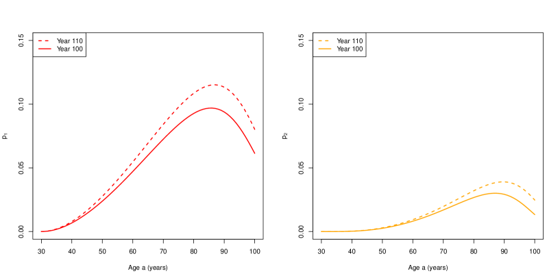
Figure 3: Age courses of $p_{1}$ (left) and $p_{2}$ (right) in the years $t=100$ (solid line) and $t=110$ (dashed lines) in simulation setting A.

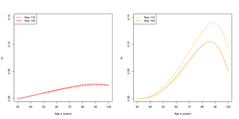
Figure 4: Age courses of $p_{1}$ (left) and $p_{2}$ (right) in the years $t=100$ (solid line) and $t=110$ (dashed lines) in simulation setting B.

In both simulation settings, A and B, we see that the prevalence of the diagnosed chronic disease is increasing from year 100 to 110 in nearly all age classes. The prevalence of the undiagnosed disease is also growing for virtually all ages in simulation A. However in setting B, the prevalence of the undiagnosed is remaining constant or slightly decreasing – despite $\lambda_{0}$ increases over time for each age group. As expected, we observe an accumulation of undetected cases in setting A and a slowly decreasing reservoir of undetected cases in setting B during the period from year 100 to year 110. By comparing the prevalences of the undiagnosed and diagnosed disease in settings A and B, we can conclude that the performance of case-finding worsens in setting A and improves in setting B.

4.2 Assessing the case-finding

4.2.1 Prevalence based figures

If we calculate the ratios $\wp_{1}$ and $\wp_{2}$ for some ages in years 100 and 110 in both simulation settings, we obtain the results as presented in Table 5. Graphical presentations are given in Figures 5 and 6.

Table 5: Age-specific detection ratios $\wp_{1}$ and $\wp_{2}$ in both simulation settings.

Age	Setting A				Setting B
(years)	$\wp_{1}$ (in %)		$\wp_{2}$ (in %)		$\wp_{1}$ (in %)		$\wp_{2}$ (in %)
	$t=100$	$t=110$	$t=100$	$t=110$	$t=100$	$t=110$	$t=100$	$t=110$
45	6.7	6.7	1.4	1.6	51	59	0.75	0.74
60	15	15	4.8	5.5	72	77	1.6	1.5
75	21	21	8.6	10	79	83	2.5	2.3
90	22	23	9.5	11	80	84	2.7	2.6

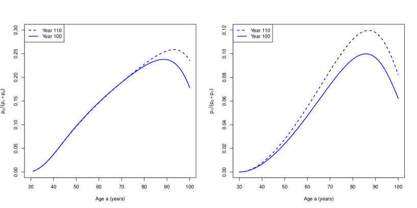
Figure 5: Age courses of the case-finding measures $\wp_{1}$ (left) and $\wp_{2}$ (right) in the years $t=100$ (solid line) and $t=110$ (dashed line) in simulation A.

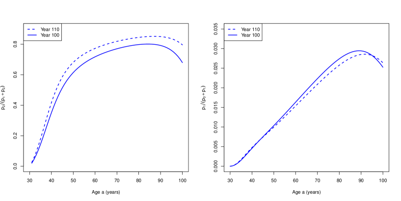
Figure 6: Age courses of the case-finding measures $\wp_{1}$ (left) and $\wp_{2}$ (right) in the years $t=100$ (solid line) and $t=110$ (dashed line) in simulation B.

In simulation setting A, we see from Table 5 and Figure 5 that for all ages the ratio $\wp_{1}$ remains the same or rises between $t=100$ and $t=110.$ For example, in the age group of 75 year-old persons, the ratio $\wp_{1}$ is 21% for both years. Thus, based on $\wp_{1}$ one would judge that the situation of case-finding remains the same and slightly improves for the higher age groups during the period 100 – 110. However if we consider $\wp_{2}$ in setting A, we get the indication that the situation worsens. For all age groups, $\wp_{2}$ increases during 100 to 110, which indicates that during that period the percentage of undiagnosed persons in the search space increases. Hence, the measures $\wp_{1}$ and $\wp_{2}$ yield contradicting findings about the performance of case-finding in the years $t=100$ and $t=110$ in simulation setting A.

In simulation setting B, Table 5 and Figure 6 show that $\wp_{1}$ indicates an improvement during the period from year 100 to year 110. $\wp_{2}$ also reveals an improvement for the ages 40 to 95.

To sum up, we can say that the figure $\wp_{2}$ assesses both settings A and B correctly, whereas $\wp_{1}$ does not value setting A as being negative with respect to case-finding..

4.2.2 Figures based on transitions between the states

Figures 7 and 8 show the age-specific detection rates $\operatorname{DR}_{0}$ and $\operatorname{DR}_{5}.$ Although different in magnitude, both measures $\operatorname{DR}_{0}$ and $\operatorname{DR}_{5}$ indicate correctly that the case-finding performance worsens from 100 to 110 in setting A and improves in setting B.

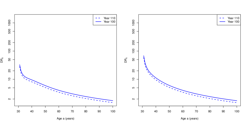
Figure 7: Age courses of the detection ratios $\operatorname{DR}_{0}$ (left) and $\operatorname{DR}_{5}$ (right) in the years $t=100$ (solid line) and $t=110$ (dashed line) in simulation setting A.

Figure 8: Age courses of the detection ratios $\operatorname{DR}_{0}$ (left) and $\operatorname{DR}_{5}$ (right) in the years $t=100$ (solid line) and $t=110$ (dashed line) in simulation setting B.

In Figure 9 we see the age courses of the $\operatorname{CDR}$ in the different simulation settings A (left) and B (right). We see that in setting A the $\operatorname{CDR}$ fails to indicate a lower performing case-finding for a wide range of ages. In setting B, the $\operatorname{CDR}$ correctly values the situation as an improvement of case-finding.

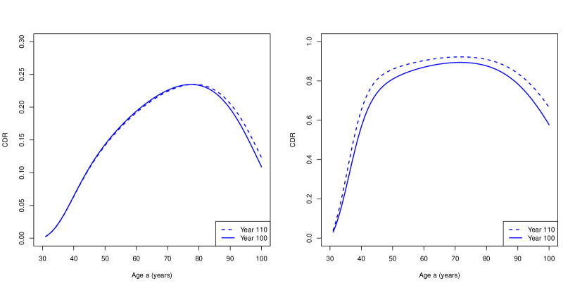
Figure 9: Age courses of the case detection ratio $\operatorname{CDR}$ in simulation setting A (left) and setting B (right) in the years $t=100$ (solid line) and $t=110$ (dashed line) in simulation setting B.

The results of assessing case-finding in the simulation settings A and B by the figure $\Phi_{5}$ are shown in Table 6. Let us consider, for example, the age group 90. In year $t=100$, out of 100,000 healthy persons 886 persons contract the undiagnosed disease. Ten years later, this number increases to 1029. Both numbers just depend on $\lambda_{0}$. Thus, they are valid for both simulation settings. Out of these 886 and 1029 incident undiagnosed cases in years 100 and 110, within five years after onset of the disease 420 and 437, respectively, die without a diagnosis in setting A. Thus, we have an increase of persons who never had the chance for a treatment, which clearly indicates a worsening of case-finding performance. In setting B, the number of these fatalities is considerably lower. In the years 100 and 110, we observe 259 and 235 death cases without diagnoses, respectively, a considerably lower number. Hence, the measure $\Phi_{5}$ indicates that the situation worsens in setting A and improves in setting B.

Table 6: Incident cases and fatalities $\Phi_{5}$ from the undiagnosed state during 5 years (per 100,000 healthy persons).

Age	Incident cases (undiagnosed)		100,000 $\Phi_{5}$
(years)	(per 100,000 healthy persons)		Setting A		Setting B
	$t=100$	$t=110$	$t=100$	$t=110$	$t=100$	$t=110$
45	222	257	1.600	1.600	0.951	0.828
60	443	514	14.11	14.12	8.202	7.109
75	665	772	89.59	90.35	52.62	46.02
90	886	1029	420.0	437.2	259.0	235.1

Table 7 sums up the findings of assessing the performance of case-finding in the different simulations settings. The measures $\wp_{1}$ and $\operatorname{CDR}$ at least partly fail to indicate the deterioration of case-finding in setting A, whereas the figures $\wp_{2}$, $\operatorname{DR}_{0}$, $\operatorname{DR}_{5}$ and $\Phi_{5}$ assess both settings correctly.

Table 7: Summary of the different measures of assessing case-finding. A plus (+) or a minus (–) sign denotes whether the measure indicates an improvement or a deterioration of case-finding over time.

Measure	Simulation A	Simulation B
$\wp_{1}$	+/–	+
$\wp_{2}$	–	+
$\operatorname{DR}_{0}$	–	+
$\operatorname{DR}_{5}$	–	+
$\operatorname{CDR}$	+/–	+
$\Phi_{5}$	–	+

5 Discussion

Based on a system of partial differential equations we set up a simulation study with an temporally increasing (setting A) and decreasing (setting B) quality of case-finding in an hypothetical chronic disease. Then, we applied different figures to assess and compare the performance of case-finding at two points in time. Some of the measures were not able to judge the differences in both simulation settings correctly. Table 7 shows how the different settings have been assessed by the different figures.

We found that the measures $\wp_{1}$ and $\operatorname{CDR}$ are unsuitable measures to assess the case-finding performance in chronic diseases, because the unfavourable situation of an temporally increasing reservoir of undiagnosed cases (setting A) has not valued as being negative.

The figure $\wp_{2}$ correctly values settings A and B. Thus, it is sensitive measure for the improvement and degradation of case-finding. Similarly, the detection ratios $\operatorname{DR}_{\gamma}$ correctly assess the different simulation settings for $\gamma=0$ and $\gamma=5.$ The figure $\Phi_{5}$ is an important measure, which refers to a cohort of healthy persons who contract the disease but never get the chance of being treated.

There are other figures to assess case-finding. For example, the mean sojourn time (MST) in the preclinical phase may be considered, see [16] for a review. Usually, a low MST is considered advantageous. However, the MST may be low if the mortality from the undiagnosed state is high. Thus, the MST is not an appropriate figure for evaluating case-finding.

Compared to the other figures, the measure $\wp_{2}=\tfrac{p_{1}}{p_{0}+p_{1}}$ has the advantage that it just require prevalence data, which can be obtained from cross-sectional studies. Those measures including the incidence rates either require costly follow-up data or the application of specialized estimation techniques [8].

In this work, we applied these measures to data about undiagnosed and diagnosed prevalence of diabetes from the KORA study. The ratio $\wp_{2}$ unveils that in men and women, the performance of case-finding is better in the age group 60–64 compared to the the age group 65–69. The reasons for this may be individual or societal, but a detailed analysis is beyond the scope of this article.

Appendix

The $\operatorname{CDR}$ is the proportion of incident cases being diagnosed [10], i.e., the notification rate of incident cases over the total incidence rate. Let $\lambda^{\prime}$ be the notification rate, which is the number of detected cases transiting from the search space to the Diagnosed state per unit time. Thus, the denominator is the number of persons in the combined state of Normal and Undiagnosed. In the model in Figure 1 the rate $\lambda_{1}$ refers to transitions from the Undiagnosed state to the Diagnosed state. Here, the denominator is the number of persons in the Undiagnosed state. Hence it holds $\lambda^{\prime}=\tfrac{p_{1}}{p_{0}+p_{1}}\,\lambda_{1}.$ As $\lambda_{0}$ is the overall incidence, it holds

$$\operatorname{CDR}=\frac{p_{1}\,\lambda_{1}}{(p_{0}+p_{1})\lambda_{0}}=\wp_{2}\,\operatorname{DR}_{0}.$$

References

- [1] Smith RA, Cokkinides V, Eyre HJ. American Cancer Society guidelines for the early detection of cancer, 2004. CA: a cancer journal for clinicians. 2004;54(1):41–52.
- [2] Mellbin LG, Anselmino M, Lars R. Diabetes, prediabetes and cardiovascular risk. European Journal of Cardiovascular Prevention & Rehabilitation. 2010;17(1 suppl):s9–s14.
- [3] Whaley-Connell A, Nistala R, Chaudhary K. The importance of early identification of chronic kidney disease. Missouri Medicine. 2010;108(1):25–28.
- [4] Gordon-Dseagu VLZ, Mindell JS, Steptoe A, Moody A, Wardle J, Demakakos P, et al. Impaired Glucose Metabolism among Those with and without Diagnosed Diabetes and Mortality: A Cohort Study Using Health Survey for England Data. PLoS ONE. 2015 03;10(3):e0119882.
- [5] Bastin A, Starling L, Ahmed R, Dinham A, Hill N, Stern M, et al. High prevalence of undiagnosed and severe chronic obstructive pulmonary disease at first hospital admission with acute exacerbation. Chronic Respiratory Disease. 2010;7(2):91–97.
- [6] Miravitlles M, Soriano JB, Garcia-Rio F, Muñoz L, Duran-Tauleria E, Sanchez G, et al. Prevalence of COPD in Spain: impact of undiagnosed COPD on quality of life and daily life activities. Thorax. 2009;64(10):863–868.
- [7] Rathmann W, Haastert B, Icks Aa, Löwel H, Meisinger C, Holle R, et al. High prevalence of undiagnosed diabetes mellitus in Southern Germany: target populations for efficient screening. The KORA survey 2000. Diabetologia. 2003;46(2):182–189.
- [8] Brinks R, Bardenheier BB, Hoyer A, Lin J, Landwehr S, Gregg EW. Development and demonstration of a state model for the estimation of incidence of partly undetected chronic diseases. BMC Medical Research Methodology. 2015;15(1):98.
- [9] Gregg EW, Cadwell BL, Cheng YJ, Cowie CC, Williams DE, Geiss L, et al. Trends in the prevalence and ratio of diagnosed to undiagnosed diabetes according to obesity levels in the US. Diabetes Care. 2004;27(12):2806–2812.
- [10] Borgdorff M. New measurable indicator for tuberculosis case detection. Emerging Infectious Diseases. 2004;10(9).
- [11] Polyanin AD, Zaitsev VF, Moussiaux A. Handbook of First-Order Partial Differential Equations. CRC Press, Boca Raton, FL; 2001.
- [12] Dahlquist G, Björck A. Numerical Methods. Prentice-Hall, Englewood Cliffs, NJ; 1974.
- [13] Carstenson B, Kristensen JK, Ottosen P, Borch-Johnsen K. The Danish National Diabetes Register: Trends in Incidence, Prevalence and Mortality. Diabetologia. 2008;51(12):2187–2196.
- [14] Preston S, Heuveline P, Guillot M. Demography: measuring and modeling population processes. Wiley-Blackwell, Malden, MA; 2000.
- [15] Finkelstein M. Discussing the Strehler-Mildvan model of mortality. Demographic Research. 2012;26(9):191–206.
- [16] Uhry Z, Hédelin G, Colonna M, Asselain B, Arveux P, Rogel A, et al. Multi-state Markov models in cancer screening evaluation: a brief review and case study. Statistical Methods in Medical Research. 2010;19(5):463–486.