High Dimensional Tests for Functional Networks of Brain Anatomic Regions

Abstract

There has been increasing interests in learning resting-state brain functional connectivity of autism disorders using functional magnetic resonance imaging (fMRI) data. The data in a standard brain template consist of over 200,000 voxel specific time series for each single subject. Such an ultra-high dimensionality of data makes the voxel-level functional connectivity analysis (involving four billion voxel pairs) lack of power and extremely inefficient. In this work, we introduce a new framework to identify functional brain network at brain anatomic region-level for each individual. We propose two pairwise tests to detect region dependence, and one multiple testing procedure to identify global structures of the network. The limiting null distributions of the test statistics are derived. It is also shown that the tests are rate optimal when the alternative networks are sparse. The numerical studies show the proposed tests are valid and powerful. We apply our method to a resting-state fMRI study on autism and identify patient-unique and control-unique hub regions. These findings are consistent with autism clinical symptoms.

Author’s Footnote:

Jichun Xie is Assistant Professor, Department of Biostatistics and Bioinformatics, Duke University School of Medicine, Durham, NC 27705. (Email: jichun.xie@duke.edu). Jian Kang is Assistant Professor, Department of Biostatistics, University of Michigan, Ann Arbor, MI 48109. (Email: jiankang@umich.edu). Jian Kang’s research was partially supported by the NIH grant R01 MH105561. The authors thank the autism brain imaging data exchange (ABIDE) study (Di Martino et al., 2013) shares the resting-state fMRI data.

Keywords: High dimensionality; Hypothesis testing; Brain network; Sparsity; fMRI study

1 Introduction

The functional brain network refers to the coherence of the brain activities among multiple spatially distinct brain regions. It plays an important role in information processing and mental representations (Bullmore and Sporns, 2009; Sporns et al., 2004), and could be altered by one’s disease status. Supekar et al. (2008); Koshino et al. (2005); Cherkassky et al. (2006) showed that patients with neurodegenerative diseases (such as the Alzheimer’s disease and the Autism Spectrum Disorder) have different function network compared with controls. As a result, the inference on functional brain network will benefit the study of these diseases. Our research goal is to infer the whole functional networks of the brain regions.

Recent advances in the neuroimaging technologies provide great opportunities for researchers to study functional brain network based on massive nueroimaging data, which are generated using various imaging modalities such as positron emission tomography (PET), functional magnetic resonance imaging (fMRI), and electroencephalography (EEG). In a neuroimaging experiment, the scanner records the brain signals over multiple times at each location (or voxel) in the three-dimensional brain, leading to a four-dimensional imaging data structure. In a typical fMRI study, the number of voxels can be up to 200,000 and the number of imaging scans over time is round 100–200. In light of the brain function and the neuroanatomy, the human brain can be partitioned to 100-200 anatomical regions and each region contains 200 to 4,000 voxels. Such high dimensionality and complexity of the data imposes great challenges on the inference of the whole brain network.

Due to the ultra-high dimensionality of voxel numbers (up to 200,000), direct inference on the network of voxels is extremely computationally expensive. More importantly, the network of interest is the network of brain regions, not voxels. To this end, Andrews-Hanna et al. (2007) examines the functional connectivity of a particular brain region, called seed region, by correlating the seed region brain signals against the brain signals from all other regions. Although this method yields a clear view of the functional connectivities between one region of interest (the seed region) and other regions (Biswal et al., 1995; Cordes et al., 2000), it fails to examine the functional network on a whole brain scale. Alternatively, Velioglu et al. (2014) proposed to form meshes around a seed voxel by regressing $p$ functionally nearest neighbor voxels on the seed voxel, where number of regressors $p$ is determined by minimizing the Akaike’s final prediction error (Akaike, 1969). Then two voxels are considered as functionally connected if one serves as a functional predictor as the other. The number of all connected voxel pairs between two anatomic regions are treated as the dependence level between these two regions. Although this method successfully provides a functional network among anatomic regions, no inference results are provided on what level of connectivities should be regarded as significant. Another commonly used method (Huang et al., 2009, 2010) is to summarize one statistic (such as the largest principal component of voxel signals) in each region and then study the dependence between these statistics. Commonly used measures of dependence include covariance matrix or Gaussian Graphical model. See Supekar et al. (2008); Weiss and Freeman (2001); Huang et al. (2009); Marrelec et al. (2006). Since only one statistic is summarized in each region, the dependence among these summarized statistics sometimes fail to represent the dependence among the regions.

In this article, we propose a new method to estimate the region-level functional connectivity for each individual. Instead of summarizing one statistic in each region, we summarize multiple statistics so that information of the region can be adequately captured. These statistics can be viewed as functional components of the region. The correlation matrix between the components in two regions are used to measure the dependence between two regions. We assume that two regions are functionally connected if and only if at least one pair of components are correlated between these two regions.

We then concatenate these functional components region by region. No region-level functional connectivity implies that the covariance matrix (or equivalently its inverse) of the concatenated components has a block-diagonal structure. This is a reasonable assumption and has been used in many existing literatures. (See Rubinov and Sporns (2010); Bowman et al. (2012); Huang et al. (2009).) Thus, to construct a functional network of brain anatomic regions, we check if the correlation matrix of two regions has a block diagonal structure.

Previous literatures for testing high dimensional covariance/correlation matrix include testing whether the covariance matrix is proportional to the identity matrix (Ledoit and Wolf, 2002; Birke and Holder, 2005; Schott, 2007; Chen et al., 2010; Cai and Ma, 2013; Li and Qin, 2014), and testing whether two covariance matrices are equal (Li and Chen, 2012; Cai et al., 2013; Li and Qin, 2014). To the best of our knowledge, no existing methods have been proposed to address whether a rectangle block of a covariance matrix is zero. However, ideas in those literatures can be borrowed to construct test statistics for our problem. There are mainly two types of existing test statistics: one is chi-square type of statistic based on the sum square of sample covariances. and the other is the extreme type of statistic based on the largest absolute self-standardized sample covariance. In general, the chi-square type of statistics performs better when the alternative network is dense and the extreme type of statistics performs better when the alternative network is sparse. In imaging studies, the network of functional components is usually sparse. Therefore, we will use the extreme type of statistics. Details will be discussed in Section 3.

The rest of the paper is organized as follows. In Section 2, we introduce the notations and define the testing hypotheses of our interests. Section 3 presents two procedures to control type I error of each hypothesis and a multiple testing procedure to control family-wise error rate. Theoretical properties of the proposed procedures are discussed in Section 4, and their numerical performances are shown in Section 6. We apply the proposed procedures on a resting-state fMRI data of subjects with and without autism spectrum disorder (ASD), and compare the functional networks of anatomic regions between cases and controls. The results match the clinical characteristics of ASD.

2 Model and Hypotheses

In fMRI studies, blood-oxygen-level dependent (BOLD) signals are collected at a large number of voxel locations for $n$ scans. The standard preprocessing steps including motion correction, slice-timing correction, normalization, de-trending and de-meaning procedures are applied to the BOLD signals (Worsley et al., 2002; Friman and Westin, 2005; Lindquist, 2008), and then the signals are clustered based on their voxel locations mapping to the existing anatomic regions. After clustering, the signals are summarized into functional components to reduce the dimension of voxels and eliminate the redundancy of high coherent signals. One way to summarize the functional components is to perform principal component analysis (PCA) in region $s$ to extract the first $q_{s}$ principal components. Alternatively, independent component analysis (ICA) can be perform to extract $q_{s}$ independent components. The choice of summarizing method depends on the distribution of the processed signals. See Anderson (2003); Richard and Yuan (2012).

For each patient, assume that $q_{s}$ functional components are summarized in region $s$. Each functional component is of length $n$, containing replications of signals across $n$ scans. After removing the temporal-correlation between the scans, denote by $X_{k,s,i}$ the $k$-th scan of the $i$-th component in $s$-th brain region. Then these components can be treated as independent across scans.

Denote by $\boldsymbol{X}_{k,s}=(X_{k,s,1},\ldots,X_{k,s,q_{s}})^{\mathrm{\scriptscriptstyle T}}$ the vector of functional components in region $s$ of scan $k$, and by

$$\boldsymbol{\Upsilon}_{st}=\textsf{Cor}(\boldsymbol{X}_{k,s},\boldsymbol{X}_{k,t})$$

the correlation matrix between region $s$ and region $t$. To test whether region $s$ and region $t$ are functionally connected, we set up the hypotheses:

$$\,\mathrm{H}_{0,st}:\boldsymbol{\Upsilon}_{st}=\boldsymbol{0},\qquad\mbox{versus}\qquad\,\mathrm{H}_{1,st}:\boldsymbol{\Upsilon}_{st}\neq\boldsymbol{0}.$$ (1)

A rejection of $H_{0,st}$ implies that regions $s$ and region $t$ have significant functional connectivity. The goal is to test $\,\mathrm{H}_{0,st}$ with controlled type I error, and also to perform multiple testing on $\,\mathrm{H}_{0,st}$ simultaneously to control family-wise error rate.

The difficulty of this testing problem lies in the large number of parameters and relatively small number of replications. First, the number of summarized functional components in each region may increase with the number of scans $n$. Second, the number of total region pairs $p(p-1)/2$ usually largely exceeds $n$. Therefore, we need to address the high dimensional challenges in testing each hypothesis and testing a large number of them simultaneously.

3 Testing Procedures

To test $\,\mathrm{H}_{0,st}$, we propose two testing procedures to fit different distribution assumptions of the functional components. Therefore, neither of them can universally outperform the other. We further develop a multiple testing procedure to control the family-wise error (FWER) for testing $\{\,\mathrm{H}_{0,st}:\ 1\leq s<t\leq p\}$ simultaneously.

3.1 Test I: Marginal Dependence Testing

The first procedure is based on the Pearson correlation between the components in two regions.

Denote by the pairwise correlation $\rho_{st,ij}=\textsf{Cor}(X_{k,s,i},X_{k,t,j})$. Then the null hypothesis $\,\mathrm{H}_{st,0}:\boldsymbol{\Upsilon}_{st}=\boldsymbol{0}$ is equivalent to $\,\mathrm{H}_{st,0}:\max_{1\leq i\leq q_{s},1\leq j\leq q_{t}}|\rho_{st,ij}|=0$. A straightforward approach is to check whether the sample correlation between two regions is close to zero. Denote the Pearson correlation between the $i$-th component in region $s$ and the $j$-th component in region $t$ by $\hat{\rho}_{st,ij}$, i.e.,

$$\hat{\rho}_{st,ij}=\hat{\sigma}_{st,ij}/\left(\hat{\sigma}_{ss,ii}\hat{\sigma}_{tt,jj}\right)^{1/2},$$

where $\bar{X}_{s,i}=\sum_{k=1}^{n}X_{k,s,i}/n$, $\bar{X}_{t,j}=\sum_{k=1}^{n}X_{k,t,j}/n$, $\hat{\sigma}_{st,ij}=\frac{1}{n}\sum_{k=1}^{n}(X_{k,s,i}-\bar{X}_{s,i})(X_{k,t,j}-\bar{X}_{t,j})$ is the sample covariance between the $i$-th component in region $s$ and the $j$-th component in region $t$, and $\hat{\sigma}_{ss,ii}$ and $\hat{\sigma}_{tt,jj}$ are sample variances defining in the similar manner. The test statistic is defined as

$$T_{st}^{(1)}=n\cdot\max_{i,j}\hat{\rho}_{st,ij}^{2}-2\log(q_{s}q_{t})+\log\log(q_{s}q_{t}).$$ (2)

With mild conditions (details in Section 4), under $\,\mathrm{H}_{0,st}$, $T_{st}^{(1)}$ asymptotically follows the Gumbel distribution

$$F(x)=\exp\{-\pi^{1/2}\exp(-x/2)\}.$$ (3)

To control type I error at level $\alpha$, we reject $\,\mathrm{H}_{0,st}$ if $T_{st}^{(1)}$ exceeds the $(1-\alpha)$-th quantile of $F(x)$, i.e., $T_{st}^{(1)}>q_{\alpha}$, with

$$q_{\alpha}=-\log(\pi)-2\log\log\{1/(1-\alpha)\}.$$ (4)

3.2 Test II: Local Conditional Dependence Testing

The alternative testing procedure is based on the Pearson correlation between the residuals of local neighborhood selection in two regions.

In region $s$, we regress on each component $X_{k,s,i}$ the rest of components,

$$X_{k,s,i}=\alpha_{s,i}+\boldsymbol{X}_{k,s,-i}^{\mathrm{\scriptscriptstyle T}}\boldsymbol{\beta}_{s,i}+\varepsilon_{k,s,i},$$ (5)

where $\boldsymbol{X}_{k,s,-i}$ is the vector of $\boldsymbol{X}_{k,s}$ by removing the $i$-th component. In region $t$ with $t\neq s$, we build up similar regression model

$$X_{k,t,j}=\alpha_{t,j}+\boldsymbol{X}_{k,t,-j}^{\mathrm{\scriptscriptstyle T}}\boldsymbol{\beta}_{t,j}+\varepsilon_{k,t,l},$$ (6)

Let $\rho_{\varepsilon,st,ij}=\textsf{Cor}(\varepsilon_{k,s,i},\varepsilon_{k,t,j})$ be the correlation of the error terms in two models. Clearly, the null hypothesis $\,\mathrm{H}_{0,st}$ is equivalent to

$$\,\mathrm{H}_{0,st}:\ \max_{i,j}\rho_{\varepsilon,st,ij}=0.$$

We therefore develop a testing procedure to test if the correlations $\rho_{\varepsilon,st,ij}$ are all zero. If the coefficients $\boldsymbol{\beta}_{s,i}$ and $\boldsymbol{\beta}_{t,j}$ in model (5) and (6) were known, we would know the value of each realization of the random error $\varepsilon_{k,s,i}$ and $\varepsilon_{k,t,j}$, and center them as $\tilde{\varepsilon}_{k,v,l}=\varepsilon_{k,v,l}-\bar{\varepsilon}_{v,l}$ with $\bar{\varepsilon}_{v,l}=\frac{1}{n}\sum_{k=1}^{n}\varepsilon_{k,v,l}$, $(v,l)=(s,i)$ or $(v,l)=(t,j)$. Based on model (5) and (6), the centered realization of randome error $\tilde{\varepsilon}_{k,v,l}$ could be expressed as

$$\tilde{\varepsilon}_{k,v,l}=X_{k,v,l}-\bar{X}_{v,l}(\boldsymbol{X}_{k,v,-l}-\bar{\boldsymbol{X}}_{v,-l})^{\mathrm{\scriptscriptstyle T}}\boldsymbol{\beta}_{v,l},\quad(v,l)=(s,i)\text{ or }(v,l)=(t,j).$$ (7)

Consequently, the Pearson correlation between $\tilde{\varepsilon}_{k,s,i}$ and $\tilde{\varepsilon}_{k,t,j}$ would be

$$\tilde{\rho}_{\varepsilon,st,ij}=\frac{1}{n}\sum_{k=1}^{n}\tilde{\sigma}_{\varepsilon,st,ij}/\left(\tilde{\sigma}_{\varepsilon,ss,ii}\tilde{\sigma}_{tt,jj}\right)^{1/2},$$

where $\tilde{\sigma}_{\varepsilon,st,ij}=\frac{1}{n}\sum_{k=1}^{n}\tilde{\varepsilon}_{k,s,i}\tilde{\varepsilon}_{k,t,j}$, $\tilde{\sigma}_{\varepsilon,ss,ii}=\frac{1}{n}\sum_{k=1}^{n}\tilde{\varepsilon}_{k,s,i}^{2}$, and $\tilde{\sigma}_{\varepsilon,tt,jj}=\frac{1}{n}\sum_{k=1}^{n}\tilde{\varepsilon}_{k,t,j}^{2}$.

Unfortunately in practice, the coefficients in (5) and (6) are unknown. However, the coefficients can be well estimated by existing methods, such as Lasso or Dantzig selector. Suppose “good” coefficient estimators $\hat{\boldsymbol{\beta}}_{s,i}$ and $\hat{\boldsymbol{\beta}}_{t,j}$ exist. Then the centered error term $\tilde{\varepsilon}_{k,v,l}$ can be estimated by

$$\hat{\varepsilon}_{k,v,l}=X_{k,v,l}-\bar{X}_{v,l}-(\boldsymbol{X}_{k,v,-l}-\bar{\boldsymbol{X}}_{v,-l})^{\mathrm{\scriptscriptstyle T}}\hat{\boldsymbol{\beta}}_{v,l},\quad(v,l)=(s,i)\text{ or }(v,l)=(t,j).$$ (8)

Consequently, we calculate Pearson correlation based on $\hat{\varepsilon}_{k,s,i}$ and $\hat{\varepsilon}_{k,t,j}$,

$$\hat{\rho}_{\varepsilon,st,ij}=\hat{\sigma}_{\varepsilon,st,ij}/\left(\hat{\sigma}_{\varepsilon,ss,ii}\hat{\sigma}_{tt,jj}\right)^{1/2},$$

where $\hat{\sigma}_{\varepsilon,st,ij}=\frac{1}{n}\sum_{k=1}^{n}\hat{\varepsilon}_{k,s,i}\hat{\varepsilon}_{k,t,j}$, $\hat{\sigma}_{\varepsilon,ss,ii}=\frac{1}{n}\sum_{k=1}^{n}\hat{\varepsilon}_{k,s,i}^{2}$, and $\hat{\sigma}_{\varepsilon,tt,jj}=\frac{1}{n}\sum_{k=1}^{n}\hat{\varepsilon}_{k,t,j}^{2}$.

Similar as Test I, we obtain the test-statistics as follows.

$$T^{(2)}_{st}=n\cdot\max_{i,j}\hat{\rho}_{\varepsilon,st,ij}^{2}-2\log(q_{s}q_{t})+\log\log(q_{s}q_{t}).$$

Under certain condtions (discussed in Section 4) and $\,\mathrm{H}_{0,st}$, $T_{st}^{(2)}$ also follows the distribution $F(x)$ in (3). Therefore, to control type I error at level $\alpha$, we reject $\,\mathrm{H}_{0,st}$ if $T^{(2)}_{st}>q_{\alpha}$, where $q_{\alpha}$ is the $(1-\alpha)$-th quantile of $F(x)$.

3.3 Family-Wise Error Rate Control

Considering the standard space of the brain (Mazziotta et al., 1995, Montreal Neurological Institute, MNI) and the commonly used brain atlas: the Automated Anatomical Labeling (Tzourio-Mazoyer et al., 2002, AAL) regions, the number of region pairs in the whole brain is over 4,000, which is much larger than the number of scans (typically a couple of hundreds). This motivates the needs of correction for multiplicity when testing any two of them are connected, in order to detect the functional connectivity of the whole brain. We propose procedure (9) to test $\{\,\mathrm{H}_{0,st}:\ 1\leq s<t\leq p\}$ simultaneously and control the family-wise error rate (fwer). The procedure can involve either $\widetilde{T}_{st}^{(1)}$ or $\widetilde{T}_{st}^{(2)}$, depending on the structure assumption of the dependence structure of local voxels. It turns out that to control fwer at level $\alpha$, we only need to adopt a higher threshold. The adjusted testing procedure is as follows:

$$\text{Reject }\,\mathrm{H}_{0,st}\text{ if and only if }T_{st}^{(b)}>2\log\{p(p-1)/2\}+q_{\alpha}\quad(1\leq s<t\leq p),$$ (9)

for $b=1,2$. The threshold depends on the desired family-wise error rate $\alpha$, and the total number of region pairs $p(p-1)/2$.

4 Theory

In this section, we show the null distributions of the test statistics in procedures I and II, their power, and the optimality properties of the proposed tests. Also, we prove that the multiple testing procedure (9) is able to control family-wise error rate.

For the rest of the paper, unless otherwise stated, we use the following notations. For a vector $\mathbf{a}=(a_{1},\ldots,a_{p})^{\mathrm{\scriptscriptstyle T}}\in\mathbb{R}^{p}$, denote by $\lvert\mathbf{a}\rvert_{2}=(\sum_{j=1}^{p}a_{j}^{2})^{1/2}$ its Euclidean norm. For a matrix $\mathbf{A}=(a_{ij})\in\mathbb{R}^{p\times q}$, define the spectral norm $\lVert\mathbf{A}\rVert_{2}=\sum_{\lvert\mathbf{x}\rvert_{2}=1}\lvert\mathbf{A}\mathbf{x}\rvert_{2}$ and the Frobenius norm $\lVert\mathbf{A}\rVert_{F}=(\sum_{ij}a_{ij}^{2})^{1/2}$. For a finite set $\mathcal{A}=\{a_{1},\ldots,a_{s}\}$, $\textsf{Card}(\mathcal{A})=s$ counts the number of elements in $\mathcal{A}$. For two real number sequences $\{a_{n}\}$ and $\{b_{n}\}$, write $a_{n}=O(b_{n})$ if $\lvert a_{n}\rvert\leq C\lvert b_{n}\rvert$ hold for a certain positive constant $C$ when $n$ is sufficiently large; write $a_{n}=o(b_{n})$ if $\lim_{n\rightarrow\infty}a_{n}/b_{n}=0$; and write $a_{n}\asymp b_{n}$ if $c\lvert b_{n}\rvert\leq\lvert a_{n}\rvert\leq C\lvert b_{n}\rvert$, for some positive constants $c$ and $C$ when $n$ is sufficiently large.

Also assume the number of variables in all regions are comparable, i.e., $q_{1}\asymp q_{2}\ldots\asymp q_{p}$. Let $q_{0}=\max(q_{1},\ldots,q_{p})$. Assume $\boldsymbol{X}_{1,v},\ldots,\boldsymbol{X}_{n,v}$ are independently and identically distributed for each region $v$.

4.1 Asymptotic Properties for Test I

Denote by $\Upsilon_{vv}=(\rho_{vv,ij})_{q_{v}\times q_{v}}$ the correlation matrix of $\boldsymbol{X}_{k,v}$. For $X_{k,v,i}$, denote by $r^{(1)}_{v,i}$ the number of other components in region $v$ that at non-negligibly correlated with $X_{k,v,i}$,

$$r^{(1)}_{v,i} =\textsf{Card}\{j:\lvert\rho_{vv,ij}\rvert\geq(\log q_{0})^{-1-\alpha_{0}},\ j\neq i\},$$

where $\alpha_{0}$ is a positive constant. For a positive constant $\rho_{0}<1$, define

$$\mathcal{D}^{(1)}_{v}=\{i:\lvert\rho_{vv,ij}\rvert>\rho_{0}\text{ for some }j\neq i\},$$

Thus, $\mathcal{D}^{(1)}_{v}$ contains index $i$ such that $X_{k,v,i}$ is highly correlated to at least one other component in region $v$.

We need the following conditions:

(C1.1) For region $v=s,t$, there exists a subset $\mathcal{M}_{v}\subset\{1,\ldots,q_{v}\}$ with $\textsf{Card}(\mathcal{M}_{v})=o(q_{v})$ and a constant $\alpha_{0}>0$ such that for all $\gamma>0$, $\max_{i\in\mathcal{M}_{v}^{c}}r^{(1)}_{v,i}=o(q_{v}^{\gamma})$. Moreover, assume there exists a constant $0\leq\rho_{0}<1$ such that $\textsf{Card}\{\mathcal{D}^{(1)}_{v}\}=o(q_{v})$.

Condition (C1.1) constraints the sparsity level of non-neglegible and large signals. It specifies that for each region $v$, for almost all component $i$ within the region, the count of non-neglible $\lvert\rho_{vv,ij}\rvert$ is of a smaller order of $q_{v}^{\gamma}$. The condition is weaker than the commonly seen condition which imposes a constant upper bound on the largest eigenvalue of $\boldsymbol{\Sigma}_{vv}$. In fact, if $\lambda_{\max}(\boldsymbol{\Sigma}_{vv})=o\{q_{v}^{\gamma}/(\log q_{0})^{1+\alpha_{0}}\}$, $\max_{1\leq i\leq q_{v}}r^{(1)}_{v,i}=o(q_{v}^{\gamma})$. In addition, (C1.1) also requires the number of components that are very highly correlated with at least one other component to be small. This condition can be easily satisfied if all the correlations $\rho_{vv,ij}$ are bounded by $\rho_{0}$.

(C1.2) Sub-Gaussian type tails: For region $v=s,t$, suppose that $\log(q_{v})=o(n^{1/5})$. There exist some constants $\eta>0$ and $K>0$ such that

$$\max_{1\leq i\leq q_{v}}\textsf{E}\left[\exp\{\eta(X_{k,v,i}-\mu_{v,i})^{2}/\sigma_{vv,ii}\}\right]\leq K.$$

(C1.2*) Polynomial-type tails: For region $v=s,t$, suppose that for some $\gamma_{1}$, $c_{1}>0$, $q_{0}\leq c_{1}n^{\gamma_{1}+1/2}$, and for some $\epsilon>0$,

$$\max_{1\leq i\leq q_{v}}\textsf{E}\lvert(X_{k,v,i}-\mu_{xi})/\sigma_{vv,ii}^{1/2}\rvert^{4\gamma_{1}+4+\epsilon}\leq K.$$

Conditions (C1.2) and C(1.2*) impose constraints on the tail of the distribution of $X_{k,v,i}$, and the corresponding order of $q_{v}$. They fit a wide rage of distributions. For example, Gaussian distribution satisfy Condition (C1.2), and Pareto distribution $Pareto(\alpha)$ (a heavy tail distribution) with $\alpha$ sufficiently large satisfy Condition (C1.2*).

(C1.3) Let $\theta_{st,ij}=\textsf{Var}\{(X_{s,i}-\mu_{s,i})(X_{t,j}-\mu_{t,j})\}$, with $\mu_{s,i}=\textsf{E}X_{s,i}$ and $\mu_{t,j}=\textsf{E}X_{t,j}$. Suppose that there exists $\kappa_{1}>0$, such that

$$\max_{1\leq i\leq q_{s},1\leq j\leq q_{t}}\frac{\sigma_{ss,ii}\sigma_{tt,jj}}{\theta_{st,ij}}\leq\kappa_{1}.$$

Condition (C1.3) holds immediately with $\kappa_{1}=1$ under the null $\,\mathrm{H}_{0,st}$, and thus we only need it for the power analysis. Under the alternative $\,\mathrm{H}_{1,st}$, it holds for a bunch of distributions. For instance, it holds when the concatenated vector $(\boldsymbol{X}_{k,s}^{\mathrm{\scriptscriptstyle T}},\boldsymbol{X}_{k,t}^{\mathrm{\scriptscriptstyle T}})^{\mathrm{\scriptscriptstyle T}}$ follows elliptically contoured distributions (Anderson, 2003). In particular, for multivariate Gaussian distributions, $\kappa_{1}\leq 2$.

We first present the asymptotic null distribution of $T_{st}^{(1)}$.

Theorem 1.

Suppose that (C1.1) and (C1.2) (or (C1.2*)) hold. Then under $\,\mathrm{H}_{0,st}$, as $n,q_{0}\rightarrow\infty$, for all $x\in\mathbb{R}$, the distribution $T_{st}^{(1)}$ converges to the Gumbel distribution $F(x)$ defined in (3).

When (C1.1) is not satisfied, i.e., the correlation matrices $\Upsilon_{ss}$ and $\Upsilon_{tt}$ are arbitrary, it is difficult to derive the limiting null distribution of $T_{st}^{(1)}$. However, Test I can still control the type I error.

Proposition 1.

Under (C1.2) (or (C1.2*)) and the null $\,\mathrm{H}_{0,st}$, for $0<\alpha<1$,

$$\textsf{P}\{T_{st}^{(1)}\geq q_{\alpha}\}\leq\log\{1/(1-\alpha)\},$$

where $q_{\alpha}$ is defined in (4).

When the desired type I error $\alpha$ is small, $\log\{1/(1-\alpha)\}\approx\alpha$. Therefore, Test I can still control type I error close to the desired level. When there comes a rare circumstance that a larger type I error is desired for the test, we can define $\alpha^{\prime}=1-\exp(-\alpha)$ and reject $\,\mathrm{H}_{0,st}$ when $\widetilde{T}_{st}^{(1)}\geq q_{\alpha^{\prime}}$. Since $\alpha=\log\{1/(1-\alpha^{\prime})\}$, Test I is always a asymptotically valid test, for arbitrary correlation matrices $\Upsilon_{ss}$ and $\Upsilon_{tt}$. However, the power will be reduced when we threshold $T_{st}^{(1)}$ at the a higher level $q_{\alpha^{\prime}}$.

We now turn to the power analysis of Test I. To test the correlation between region $s$ and region $t$, we define the following class of correlation matrix:

$$\mathcal{U}_{st}^{(1)}(c)=\left\{\Upsilon_{st}:n\cdot\max_{i,j}\rho_{st,ij}^{2}\geq c\log d_{st}\right\},$$

It turns out that Test I distinguishes $\Upsilon_{st}$ in $\mathcal{U}_{st}^{(1)}\{4(1+\kappa_{1})\}$ from a zero matrix with a probability approaching to one asymptotically.

Theorem 2.

Suppose that (C1.2) (or (C1.2*)) and (C1.3) hold. Then as $n$ and $q_{0}$ both go to infinity,

$$\inf_{\Upsilon_{st}\in\mathcal{U}_{st}^{(1)}\{4(1+\kappa_{1})\}}\textsf{P}\{T_{st}^{(1)}>q_{\alpha}\}\rightarrow 1.$$

To distinguishes the alternative from the null, Test I requires only one entry in the correlation matrix $\Upsilon_{st}$ larger than $(c\log d_{st}/n)^{1/2}$. The rate is optimal in terms of the following minimax argument. Denote by $\mathcal{F}_{st}^{(1)}$ the collection of distributions satisfying (C1.2) or (C1.2*), and by $\mathcal{T}_{st,\alpha}^{(1)}$ the collection of all $\alpha$-level tests over $\mathcal{F}_{st}^{(1)}$, i.e.,

$$\text{For all }\Phi_{st,\alpha}\in\mathcal{T}_{st,\alpha}^{(1)},\quad\textsf{P}\{\Phi_{st,\alpha}=1\}\leq\alpha.$$

Theorem 3 shows that, if the maximum absolute correlation is less than $(c_{0}\log d_{st}/n)^{1/2}$, for some $c_{0}$, no test can perfectly distinguish the alternative from the null. Thus, Theorems 2 and 3 together indicate that Test I has certain rate optimality property.

Theorem 3.

Suppose (C1.2) or (C1.2*) holds. Let $\alpha$ and $\beta$ be any positive numbers with $\alpha+\beta<1$. There exists a positive constant $c_{0}$ such that for all large $n$ and $q_{0}$,

$$\inf_{\Upsilon_{st}\in\mathcal{U}_{st}^{(1)}(c_{0})}\sup_{T_{st,\alpha}\in\mathcal{T}_{st,\alpha}^{(1)}}\textsf{P}(T_{st,\alpha}=1)\leq 1-\beta.$$

In Theorem 2 and 3, the difference between the null and the alternative is measured by the maximal absolute value of the entries in $\Upsilon_{st}$. Another commonly used measure is the Frobenius norm $\lVert\Upsilon_{st}\rVert_{F}$. Denote by $r_{st}$ the count of the nonzero entries in $\Upsilon_{st}$, i.e.,

$$r_{st}=\sum_{i=1}^{q_{s}}\sum_{j=1}^{q_{t}}I(\rho_{st,ij}\neq 0).$$

Consider the following class of matrices:

$$\mathcal{V}_{st}^{(1)}(c)=\left\{\Upsilon_{st}:\ \lVert\Upsilon_{st}\rVert_{F}^{2}\geq cr_{st}\log d_{st}/n\right\}.$$

We now show that Test I enjoys the rate optimality property measured by Frobenius norm too.

Corollary 1.

Suppose that (C1.2) or (C1.2*) holds. Then for a sufficiently large $c$, as $n$ and $q_{0}$ both go to infinity,

$$\inf_{\Upsilon_{st}\in\mathcal{V}_{st}^{(1)}(c)}\textsf{P}\{T_{st}^{(1)}>q_{\alpha}\}\rightarrow 1.$$

Theorem 4.

Suppose that (C1.2) or (C1.2*) holds. Assume that $r_{st}\leq q_{0}^{\gamma_{2}}$ for some $0<\gamma_{2}<1/2$. Let $\alpha,\beta$ be any positive number with $\alpha+\beta<1$. There exists a positive contant $c_{0}$ such that for all large $n$ and $q_{0}$,

$$\inf_{\boldsymbol{\Sigma}_{st}\in\mathcal{V}_{st}^{(1)}(c_{0})}\sup_{T_{st,\alpha}\in\mathcal{T}_{st,\alpha}^{(1)}}\textsf{P}(\Phi_{st,\alpha}=1)\leq 1-\beta.$$

In Theorem 4, we assume that $r_{st}\leq q_{0}^{\gamma_{2}}$. The assumption is quite reasonable for brain network, because if the connections of the functional components exist between two brain regions, they are usually sparse.

4.2 Asymptotic Properties for Test II

For Test II, the conditions required for achieving its asymptotic property are different from what required for Test I.

Recall that $\varepsilon_{k,s,i}$ and $\varepsilon_{k,t,j}$ are the error term of regressing all other components on one component within the region, as defined in (5) and (6), and $\sigma_{\varepsilon,st,ij}=\textsf{Cov}(\varepsilon_{k,s,i},\varepsilon_{k,t,j})$. Let $\Upsilon_{\varepsilon,st}=(\rho_{\varepsilon,st,ij})$ be the correlation matrix between $\boldsymbol{\varepsilon}_{k,s}=(\varepsilon_{k,s,1},\ldots,\varepsilon_{k,s,q_{s}})^{\mathrm{\scriptscriptstyle T}}$ and $\boldsymbol{\varepsilon}_{k,t}=(\varepsilon_{k,t,1},\ldots,\varepsilon_{k,t,q_{t}})^{\mathrm{\scriptscriptstyle T}}$. Then

$$\rho_{\varepsilon,st,ij}=\frac{\sigma_{\varepsilon,st,ij}}{(\sigma_{\varepsilon,ss,ii}\sigma_{\varepsilon,tt,jj})^{1/2}},$$

where $\sigma_{\varepsilon,st,ij}=\textsf{Cov}(\varepsilon_{k,s,i},\varepsilon_{k,t,j})$, $\sigma_{\varepsilon,ss,ii}=\textsf{Var}(\varepsilon_{k,s,i})$ and $\sigma_{\varepsilon,tt,jj}=\textsf{Var}(\varepsilon_{k,t,j})$.

For $\varepsilon_{k,s,i}$, denote by $r^{(2)}_{v,i}$ the number of other $\varepsilon_{k,s,j}$ that are non-negligibly correlated ($>(\log q_{0})^{-1-\alpha_{0}}$) with it,

$$r^{(2)}_{v,i}=\textsf{Card}\{j:\ \lvert\rho_{\varepsilon,vv,ij}\rvert\geq(\log q_{0})^{-1-\alpha_{0}},\ j\neq i\}.$$

For a positive constant $\rho_{0}<1$, define the following set that $\varepsilon_{k,v,i}$ is highly correlated with at least one $\varepsilon_{k,v,j}$ as

$$\mathcal{D}^{(2)}_{v}=\{i:\lvert\rho_{\varepsilon,vv,ij}\rvert>\rho_{0}\text{ for some }j\neq i\}.$$

We need the following conditions:

(C2.1) For regions $v=s,t$, there exists a subset $\mathcal{M}_{v}\in\{1,\ldots,q_{v}\}$ with $\textsf{Card}(\mathcal{M}_{v})=o(q_{v})$ and a constant $\alpha_{0}>0$ such that all $\gamma>0$, $\max_{1\leq i\leq p,i\in\mathcal{M}_{v}}r^{(2)}_{v,i}=o(q_{v}^{\gamma})$. Moreover, assume there exists a constant $0\leq\rho_{0}<1$ such that $\textsf{Card}\{\mathcal{D}_{v}\}=o(q_{0})$.

Condition (C2.1) parallels with Condition (C1.1). It imposes conditions on the within region correlation $\boldsymbol{\Upsilon}_{\varepsilon,vv}$. Suppose $\boldsymbol{X}_{k,v}$ follow multivariate Gaussian distribution with $\boldsymbol{\Omega}_{vv}=(\omega_{vv,ij})$ to be its inverse covariance matrix. Because $\rho_{\varepsilon,vv,ij}=\omega_{vv,ij}/(\omega_{vv,ii}\omega_{vv,jj})^{1/2}$ (Anderson, 2003), Condition (C2.1) holds under many cases when inverse covariance matrix of the components are sparse and bounded. See Honorio et al. (2009); Huang et al. (2010); Mazumder and Hastie (2012). Obviously, the covariance matrix and inverse covariance matrix are different, and consequently many data only satisfy one of these two conditions, and then the corresponding procedure should be applied to the data.

(C2.2) For region $v=s,t$, the variable $\boldsymbol{X}_{k,v}\sim\mathrm{N}(\boldsymbol{\mu}_{v},\boldsymbol{\Sigma}_{vv})$, with $\lambda_{\max}(\boldsymbol{\Sigma}_{vv})\leq c_{0}$, where $\lambda_{\max}$ is the maximum eigenvalue operator. Also assume $\log q_{0}=o(n^{1/5})$.

In general, the theoretical properties of Test II hold for many non-Gaussian distributions as well. However, only under the Gaussian distribution assumption, $\rho_{\varepsilon,vv,ij}$ has an interpretation of conditional dependence such that

$$\rho_{\varepsilon,vv,ij}=0\text{ if and only if }X_{k,v,i}\mathchoice{\mathrel{\hbox to0.0pt{$\displaystyle\perp$\hss}\mkern 2.0mu{\displaystyle\perp}}}{\mathrel{\hbox to0.0pt{$\textstyle\perp$\hss}\mkern 2.0mu{\textstyle\perp}}}{\mathrel{\hbox to0.0pt{$\scriptstyle\perp$\hss}\mkern 2.0mu{\scriptstyle\perp}}}{\mathrel{\hbox to0.0pt{$\scriptscriptstyle\perp$\hss}\mkern 2.0mu{\scriptscriptstyle\perp}}}X_{k,v,j}\mid\{X_{k,v,l},\ l\neq i,j\}.$$

Condition (C2.2) makes Condition (C2.1) a natrual assumption on the conditional dependency. Since $\sigma_{vv,ii}\leq\lambda_{\max}(\boldsymbol{\Sigma}_{vv})$ and $\sigma_{vv,ii}\omega_{vv,ii}\geq 1$, this condition also implies that $\textsf{Var}(\varepsilon_{k,s,i})=1/\omega_{vv,ii}\leq c_{0}$.

(C2.3) Recall the definition of $\tilde{\varepsilon}_{k,v,l}$ and $\hat{\varepsilon}_{k,v,l}$ in (7) and (8). Under the cases (i) $s\neq t$ and (ii) $s=t$ and $i=j$, with probability tending to one,

$$\max_{i,j}\left\lvert\frac{1}{n}\sum_{k=1}^{n}\hat{\varepsilon}_{k,s,i}\hat{\varepsilon}_{k,t,j}-\frac{1}{n}\sum_{k=1}^{n}\tilde{\varepsilon}_{k,s,i}\tilde{\varepsilon}_{k,t,j}\right\rvert\leq C(\log q_{0})^{-1-\alpha_{0}}.$$ (10)

Note that $\hat{\varepsilon}_{k,v,i}$ is the centered residual and $\tilde{\varepsilon}_{k,v,i}$ is the centered random error. The term $\lvert\frac{1}{n}\sum_{k=1}^{n}\hat{\varepsilon}_{k,s,i}\hat{\varepsilon}_{k,t,j}-\frac{1}{n}\sum_{k=1}^{n}\tilde{\varepsilon}_{k,s,i}\tilde{\varepsilon}_{k,t,j}\rvert$ is determined by the difference between $\boldsymbol{\beta}_{v,i}$ and its estimator $\hat{\boldsymbol{\beta}}_{v,i}$. We will specify in Section 5 some estimation methods and corresponding sufficient conditions under which Condition (C2.3) will hold.

Theorem 5 specifies the null distribution of $T_{st}^{(2)}$.

Theorem 5.

Suppose that (C2.1), (C2.2) and (C2.3) hold. Then under $\,\mathrm{H}_{0}$, as $n,q_{0}\rightarrow\infty$, for all $v\in\mathbb{R}$, $T_{st}^{(2)}$ weakly converges to the Gumbel distribution $F(x)$ in (3).

The derivation of the limiting null distribution of $T_{st}^{(2)}$ calls for Condition (C2.1); when it is not satisfied, we can still control type I error based on the following proposition.

Proposition 2.

Under (C2.2) and (C2.3) and the null $\,\mathrm{H}_{0,st}$,

$$\textsf{P}\{T_{st}^{(2)}\geq q_{\alpha}\}\leq\log\left\{1/(1-\alpha)\right\},$$

where $q_{\alpha}=-log(\pi)-2\log\log\{1/(1-\alpha)\}$ is the $(1-\alpha)$-th quantile of $F(x)$ defined in (3).

The power analysis of Test II parallels to that of Procedure I. Let $r_{\varepsilon,st}=\sum_{i=1}^{q_{s}}\sum_{j=1}^{q_{t}}I(\rho_{\varepsilon,st,ij}\neq 0)$. Define the following two classes of matrices:

$$\mathcal{U}_{st}^{(2)}(c) =\left\{\Upsilon_{\varepsilon,st}:\ \max_{1\leq i\leq q_{s},1\leq j\leq q_{t}}\rho^{2}_{\varepsilon,st,ij}\geq c\log d_{st}/n\right\};$$

$$\mathcal{V}_{st}^{(2)}(c) =\left\{\Upsilon_{\varepsilon,st}:\ \lVert\Upsilon_{\varepsilon,st}\rVert_{F}^{2}\geq cr_{\varepsilon,st}\log d_{st}/n\right\}.$$

We have the following theorem.

Theorem 6.

Suppose that (C2.2), and (C2.4) hold. Then

$$\lim_{n,q_{0}\rightarrow\infty}\inf_{\mathbf{R}_{st}\in\mathcal{U}_{st}^{(2)}(c_{1})}\textsf{P}\left\{T_{st}^{(2)}\geq q_{\alpha}\right\}=1,\quad\text{and }\lim_{n,p\rightarrow\infty}\inf_{\mathbf{R}_{st}\in\mathcal{V}_{st}^{(2)}(c_{2})}\textsf{P}\left\{T_{st}^{(2)}\geq q_{\alpha}\right\}=1,$$

for some $c_{2}\geq c_{1}$.

Similar as Test I, Test II enjoys certain rate optimality in its power. Denote by $\mathcal{F}_{st}^{(2)}$ the collection of distributions satisfying (C2.2), and by $\mathcal{T}^{(2)}_{st,\alpha}$ the collection of all $\alpha$-level test over $\mathcal{F}_{st}^{(2)}$.

Theorem 7.

Suppose (C2.2) holds. Let $\alpha,\beta$ be any positive number with $\alpha+\beta<1$, There exists a positive constant $c_{3}$ such that for all large $n$ and $q_{0}$,

$$\inf_{\mathbf{R}_{\varepsilon,st}\in\mathcal{U}_{st}^{(2)}(c_{3})}\sup_{\Phi_{st,\alpha}\in\mathcal{T}_{st,\alpha}^{(2)}}\textsf{P}(\Phi_{st,\alpha} =1)\leq 1-\beta;$$

$$\inf_{\mathbf{R}_{\varepsilon,st}\in\mathcal{V}_{st}^{(2)}(c_{3})}\sup_{\Phi_{st,\alpha}\in\mathcal{T}_{st,\alpha}^{(2)}}\textsf{P}(\Phi_{st,\alpha} =1)\leq 1-\beta.$$

4.3 Asymptotic Properties for Multiple Testing Procedure

The properties of the the multiple testing procedure (9) are based on the limiting null distribution of each test statistic. Based on Theorems 1 and 5, we have the following results.

Theorem 8.

Consider the multiple testing procedure (9). If (C1.1) and (C1.2) (or (C1.2*)) hold, the procedure (9) with $T_{st}^{(1)}$ controls the family-wise error rate at level $\alpha$. If (C2.1) and (C2.2) hold, the procedure with $T_{st}^{(2)}$ controls the family-wise error rate at level $\alpha$.

5 Estimation of $\widehat{\boldsymbol{\beta}}_{v,i}$

Test II depends on the estimators of regression model. Estimating regression coefficients has been investigated extensively in the past several decades; methods include the Dantzig selector (Candes and Tao, 2007), the Lasso (Tibshirani, 1996), the SCAD (Fan and Li, 2001), the adaptive Lasso (Zou, 2006), the Scaled-Lasso (Sun and Zhang, 2012), the Square-root Lasso (Belloni et al., 2011), etc.. In this paper, we focus on the Dantzig selector and Lasso, and discuss when they will yield good estimators than can be used for our testing procedures. In particular, we will discuss the necessary conditions for (C2.3) to hold.

Before we discuss the estimating methods, we introduce the following notations. For region $v$ and component $i$, let $\mathbf{b}_{v,i}=\frac{1}{n}\sum_{k=1}^{n}(\boldsymbol{X}_{k,v,-i}-\bar{\boldsymbol{X}}_{v,-i})^{\mathrm{\scriptscriptstyle T}}(X_{k,v,i}-\bar{X}_{v,i})$ be the sample covariance between this components and other components in the region. Denote by $\hat{\boldsymbol{\Sigma}}_{vv,-i,-i}=\frac{1}{n}\sum_{k=1}^{n}(\boldsymbol{X}_{k,v,-i}-\bar{\boldsymbol{X}}_{v,-i})(\boldsymbol{X}_{k,v,-j}-\bar{\boldsymbol{X}}_{v,-j})^{\mathrm{\scriptscriptstyle T}}$ the sample covariance matrix without component $i$, and let $\mathbf{D}_{v,i}=\textsf{diag}(\hat{\boldsymbol{\Sigma}}_{vv,-i,-i})$. For the following methods, the tuning parameters are

$$\lambda_{v,i}(\delta)=\delta(\hat{\sigma}_{vv,ii}\log q_{v}/n)^{1/2}.$$

Dantzig Selector. For $v=1,\ldots,p$ and $i=1,\ldots,q_{v}$, the Danztig selector estimators are obtained by

$$\hat{\boldsymbol{\beta}}_{v,i}(\delta)=\arg\min\lvert\boldsymbol{\alpha}\rvert_{1},\quad\text{subject to }\lvert\mathbf{D}_{v,i}^{-1/2}\hat{\boldsymbol{\Sigma}}_{-i,-i}\boldsymbol{\alpha}-\mathbf{D}_{v,i}^{-1/2}\mathbf{b}_{v,i}\rvert_{\infty}\leq\lambda_{v,i}(\delta).$$ (11)

Lasso. For $v=1,\ldots,p$ and $i=1,\ldots,q_{v}$, the Lasso estimators are obtained by

$$\hat{\boldsymbol{\beta}}_{v,i}(\delta)=\mathbf{D}_{v,i}^{-1/2}\hat{\boldsymbol{\alpha}}_{v,i}(\delta),\\ \text{where }\hat{\boldsymbol{\alpha}}_{v,i}(\delta)=\arg\min_{\boldsymbol{\alpha}\in\mathbb{R}^{p-1}}\left[\frac{1}{2n}\sum_{k=1}^{n}\left\{X_{k,v,i}-\bar{X}_{v,i}-(\boldsymbol{X}_{k,v,-i}-\bar{\boldsymbol{X}}_{v,-i})\mathbf{D}_{v,i}^{-1/2}\boldsymbol{\alpha}\right\}^{2}+\lambda_{v,i}(\delta)\lvert\boldsymbol{\alpha}\rvert_{1}\right].$$ (12)

We now demonstrate that under certain conditions, the methods yield good estimators that satisfy the need to testing. Define by $a_{v,1}$ and $a_{v,2}$ the error bound

$$a_{v,1}=\max_{1\leq i\leq q_{v}}\lvert\hat{\boldsymbol{\beta}}_{v,i}-\boldsymbol{\beta}_{v,i}\rvert_{1},\quad a_{v,2}=\max_{1\leq i\leq q_{v}}\lvert\hat{\boldsymbol{\beta}}_{v,i}-\boldsymbol{\beta}_{v,i}\rvert_{2}$$ (13)

Proposition 3.

Suppose that (C2.2) holds. Consider the Dantzig selector estimator $\hat{\boldsymbol{\beta}}_{v,i}(2)$ in (11). Then if $\max_{1\leq i\leq q_{v}}\lvert\boldsymbol{\beta}_{v,i}\rvert_{0}=o\left\{n(\log q_{0})^{-3-2\alpha_{0}}[\lambda_{\min}(\boldsymbol{\Sigma})]^{2}\right\}$, then Condition (C2.3) holds.

Proposition 4.

Suppose that (C2.2) holds. Consider the Lasso estiamtor $\hat{\boldsymbol{\beta}}_{v,i}(2.02)$ in (12). Then if $\max_{1\leq i\leq q_{v}}\lvert\boldsymbol{\beta}_{v,i}\rvert_{0}=o\left\{n(\log q_{0})^{-3-2\alpha_{0}}[\lambda_{\min}(\boldsymbol{\Sigma})]^{2}\right\}$, Condition (C2.3) holds.

In fact, Proposition 3 holds for any Dantzig selector estimator $\hat{\boldsymbol{\beta}}_{v,i}(\delta)$ with $\delta\geq 2$; and Proposition 4 holds for any Lasso estimator $\hat{\boldsymbol{\beta}}_{v,i}(\delta)$ with $\delta>2$. For computational simplicity, we chose $\delta=2.02$. In numerical studies, we found such choice work well in testing.

6 Simulation Studies

In this section, we evaluate the performance of the our methods via two simulation studies: one is focused on the size and power of the proposed tests for two regions, the other illustrates how to identity the functional brain network using the proposed tests under family-wise error rate controls.

6.1 Size and Power

We simulate $\boldsymbol{X}_{k}$, for $k=1,\ldots,n$, from a normal distribution with mean zero and covariance $\boldsymbol{\Sigma}_{11,22}$, i.e.

$$\boldsymbol{X}_{k}\sim\mathrm{N}(\boldsymbol{0}_{q_{1}+q_{2}},\boldsymbol{\Sigma}_{11,22})\quad\mbox{ with }\quad\boldsymbol{\Sigma}_{11,22}=\left(\begin{array}[]{cc}\boldsymbol{\Sigma}_{11}&\boldsymbol{\Sigma}_{12}\\ \boldsymbol{\Sigma}^{\mathrm{\scriptscriptstyle T}}_{12}&\boldsymbol{\Sigma}_{22}\end{array}\right),$$

where $\boldsymbol{X}_{k}=(\boldsymbol{X}^{\mathrm{\scriptscriptstyle T}}_{k,1},\boldsymbol{X}^{\mathrm{\scriptscriptstyle T}}_{k,2})^{\mathrm{\scriptscriptstyle T}}$ and $\boldsymbol{X}_{k,s}$ is of dimension $q_{s}$ for $s=1,2$. For comparisons, we also consider a simple test for $\,\mathrm{H}_{0,12}$ in (1) based on the Person correlation coefficient between the principal component scores. Specifically, denote by ${\mathbf{Z}}_{s}$ the first principal component score of data $(\boldsymbol{X}^{\scriptsize{\mathrm{T}}}_{1,s},\ldots,\boldsymbol{X}^{\scriptsize{\mathrm{T}}}_{n,s})^{\scriptsize{\mathrm{T}}}$. We compute the sample correlation between ${\mathbf{Z}}_{1}$ and ${\mathbf{Z}}_{2}$, denoted $\widehat{\rho}_{12}$. The Fisher’s Z transformation is then taken to obtain the testing statistics $T^{(3)}_{12}$ for this simple approach, which is given by

$$T^{(3)}_{12}=\frac{1}{2}\log\left(\frac{1+\widehat{\rho}_{12}}{1-\widehat{\rho}_{12}}\right).$$

Using the results by  Hotelling (1953), it is straightforward to show that $\sqrt{n-3}T^{(3)}_{12}\rightarrow N(0,1)$ under $\,\mathrm{H}_{0,12}$ in (1). This implies that we reject $\,\mathrm{H}_{0,12}$ if $\sqrt{n-3}|T^{(3)}_{12}|>z_{\alpha/2}$, where $z_{\alpha}$ is the $1-\alpha$ normal quantile. We refer to this testing procedure as test III.

To define different model specifications on $\boldsymbol{\Sigma}_{11,22}$, we introduce a few auxiliary matrices. Let $\mathbf{A}_{d}=(a_{ij})_{d\times d}$ where $a_{ii}=1$ and $a_{ij}\sim 0.5\mbox{Bernoulli}(0.5)$ for $10(k-1)+1\leq i\neq j\leq 10k$, where $k=1,\ldots,[d/10]$ and $a_{ij}=0$ otherwise. Let $\mathbf{B}_{d}=(b_{ij})_{d\times d}$ where $b_{ii}=1$, $b_{i,i+1}=b_{i-1,i}=0.5$ and $b_{i,j}=0$ for $|i-j|>3$.

Let $\boldsymbol{\Lambda}_{d}=(\lambda_{ij})_{d\times d}$ with $\lambda_{ii}\sim\,\mathrm{U}(0.5,2.5)$ and $\lambda_{ij}=0$ for $i\neq j$. Now, we define four different models for $\boldsymbol{\Sigma}_{11}$ and $\boldsymbol{\Sigma}_{22}$.

• Model 1 (Independent Cases): $\boldsymbol{\Sigma}_{ss}=\boldsymbol{\Lambda}_{q_{s}}$, for $s=1,2$.

• Model 2 (Block Sparse Covariance Matrices): $\boldsymbol{\Sigma}_{ss}=\boldsymbol{\Lambda}^{1/2}_{q_{s}}(\mathbf{A}_{q_{s}}+\delta_{i}\mathbf{I}_{q_{s}})/(1+\delta_{i})\boldsymbol{\Lambda}^{1/2}_{q_{s}}$, for $s=1,2$, where $\delta_{i}=|\lambda_{\mathrm{m}in}(\mathbf{A}_{q_{s}})|+0.05$.

• Model 3 (Block Sparse Precision Matrices): $\boldsymbol{\Sigma}_{ss}=\boldsymbol{\Lambda}^{1/2}_{q_{s}}(\mathbf{A}^{-1}_{q_{s}}+\delta^{*}_{i}\mathbf{I}_{q_{s}})/(1+\delta^{*}_{i})\boldsymbol{\Lambda}^{1/2}_{q_{s}}$, for $s=1,2$, where $\delta^{*}_{i}=|\lambda_{\mathrm{m}in}(\mathbf{A}^{-1}_{q_{s}})|+0.05$.

• Model 4 (Binded Sparse Covariance Matrices): $\boldsymbol{\Sigma}_{ss}=\boldsymbol{\Lambda}^{1/2}_{q_{s}}(\mathbf{B}_{q_{s}}+\tau_{s}\mathbf{I}_{q_{s}})/(1+\tau_{s})\boldsymbol{\Lambda}^{1/2}_{q_{s}}$, for $s=1,2$, where $\tau_{s}=|\lambda_{\mathrm{m}in}(\mathbf{B}_{q_{s}})|+0.05$.

• Model 5 (Binded Sparse Precision Matrices): $\boldsymbol{\Sigma}_{ss}=\boldsymbol{\Lambda}^{1/2}_{q_{s}}(\mathbf{B}^{-1}_{q_{s}}+\tau^{*}_{s}\mathbf{I}_{q_{s}})/(1+\tau^{*}_{s})\boldsymbol{\Lambda}^{1/2}_{q_{s}}$, for $s=1,2$, where $\tau^{*}_{s}=|\lambda_{\mathrm{m}in}(\mathbf{B}^{-1}_{q_{s}})|+0.05$.

To simulate the empirical size, we assume $\boldsymbol{\Sigma}_{12}=\boldsymbol{0}_{q_{1}\times q_{2}}$. To evaluate the empirical power, let $\boldsymbol{\Sigma}_{12}=(\sigma_{ij})_{q_{1}\times q_{2}}$ with $\sigma_{ij}\sim s_{ij}\mbox{Bernoulli}[5/(q_{1}q_{2})]$ with $s_{ij}\sim\mathrm{N}(4\sqrt{\log(q_{1}q_{2})/n},0.5)$. The sample size is taken to be $n=80$ and $150$, while the dimension $(q_{1},q_{2})$ varies over $(50,50)$, $(100,150)$, $(200,200)$ and $(250,300)$. The nominal significant level for all the tests is set at $\alpha=0.05$. The empirical sizes and powers for the five Models, reported in Tables 1 and 2, are estimated from 5,000 replications.

Obviously when the covariance matrix of each region is sparse, Test I controls the type I error better; and when the precision matrix is sparse, Test II controls the type I error better. This implies the essence of condition (C1.1) and (C2.1) when deriving the limiting null distribution. On the other hand, the simulation also shows that without these two conditions, there is very little inflation in the type I error. The power analysis shows the similar pattern. In general, Test I/II has a larger power when the covariance/precision matrix is sparse. Both Tests I and II achieve a much larger power than Test III (Person correlation test on the first PC scores), although the empirical sizes of Test III are comparable to the proposed tests.

Table 1: Empirical size of Tests I, II and III for different sample sizes and models ($\times 10^{-2}$)

Model	Test	$(q_{1},q_{2})$
		(30,30)	(50,50)	(100,150)	(200,200)	(300,250)
				$n=80$
1	I	4.50	4.46	4.54	5.14	6.16
	II	4.58	4.48	4.70	5.70	5.44
	III	6.48	6.26	3.38	5.34	7.60
2	I	4.20	4.60	4.52	6.04	6.06
	II	2.88	4.06	4.08	3.86	2.88
	III	6.46	4.58	8.88	7.34	6.32
3	I	3.44	4.02	4.50	4.98	3.20
	II	4.56	3.94	5.02	5.76	5.74
	III	8.26	3.36	7.40	6.38	3.48
4	I	4.80	4.82	5.12	5.22	6.02
	II	1.92	2.28	3.04	2.16	3.12
	III	4.42	3.36	6.56	4.78	3.20
5	I	0.88	1.02	1.06	1.90	1.90
	II	4.52	4.60	4.32	6.28	6.14
	III	4.52	4.28	5.38	4.36	6.40
				$n=150$
1	I	4.94	4.10	5.04	4.62	4.84
	II	4.76	4.34	4.78	5.18	5.36
	III	8.80	4.04	6.44	5.56	5.76
2	I	5.08	4.62	4.48	4.88	4.74
	II	4.02	4.68	4.40	4.70	4.24
	III	5.86	7.46	3.30	4.04	5.02
3	I	4.94	4.68	4.50	4.86	4.60
	II	5.34	4.68	4.26	5.12	5.04
	III	2.76	8.80	4.74	5.22	3.98
4	I	5.02	4.78	4.96	4.92	5.10
	II	2.62	2.46	3.62	3.42	3.78
	III	2.92	5.74	6.50	5.52	4.00
5	I	1.96	1.92	1.96	2.18	3.10
	II	5.62	4.46	4.04	4.92	4.94
	III	3.38	5.92	3.90	5.42	2.34

Table 2: Empirical power of Tests I, II and III for different sample sizes and models ($\times 10^{-2}$)

Model	Test	$(q_{1},q_{2})$
		(30,30)	(50,50)	(100,150)	(200,200)	(300,250)
				$n=80$
1	I	88.58	85.00	60.20	55.44	54.74
	II	88.46	85.46	60.36	55.84	54.04
	III	11.32	6.26	7.06	8.66	6.18
2	I	88.04	80.20	59.78	55.08	55.10
	II	69.72	64.10	49.70	44.72	43.94
	III	6.46	4.00	7.00	5.72	7.28
3	I	69.88	65.50	50.24	44.40	44.36
	II	87.46	80.40	59.30	54.94	55.90
	III	3.84	3.36	7.80	4.50	3.96
4	I	90.24	95.42	63.40	56.08	64.32
	II	56.82	59.16	43.98	42.18	42.84
	III	8.02	8.52	10.12	5.96	8.64
5	I	80.82	75.14	44.30	35.00	34.78
	II	89.94	85.36	54.30	49.90	44.96
	III	8.12	5.30	6.52	6.68	7.60
				$n=150$
1	I	98.82	98.08	96.66	89.24	85.22
	II	98.96	98.04	96.98	87.78	85.04
	III	13.82	4.04	8.82	7.52	9.48
2	I	99.14	97.86	97.02	87.62	84.46
	II	86.98	75.92	73.30	55.58	55.18
	III	8.10	11.48	6.26	5.02	3.64
3	I	90.06	87.74	76.38	54.88	55.48
	II	94.58	94.70	92.48	84.80	79.94
	III	3.80	9.26	4.26	5.84	3.04
4	I	95.26	92.56	88.68	74.92	85.42
	II	85.40	67.54	64.48	58.32	59.26
	III	9.34	10.14	9.24	6.56	6.08
5	I	84.74	79.74	56.00	44.96	45.40
	II	95.10	89.96	78.44	55.24	53.32
	III	7.94	9.08	5.26	3.62	2.34

6.2 Network Identifications

In this section, we perform the simulation studies to illustrate the performance of our proposed testing procedure with the family-wise error rate control on the network identifications. We simulate a region-level brain network according to the Erdös-Rényi model (Erdös and Rényi, 1960). We set the number of regions $p=90$, and the probability of any two brain regions being functional connected as $0.01$. The simulated brain network is shown in Figure 1 in the supplementary document.

For every two connected brain regions $s$ and $t$ on the simulated network, we consider four models that we discussed in Section 6.1 for the specifications of $\boldsymbol{\Sigma}_{ss}$ and $\boldsymbol{\Sigma}_{tt}$. Similar to the simulation studies for evaluating the empirical power, we set $\boldsymbol{\Sigma}_{st}=(\sigma_{ij})_{q_{s}\times q_{t}}$ with $\sigma_{ij}\sim s_{ij}\mbox{Bernoulli}(10/d_{st})$ with $s_{ij}\sim\mathrm{N}(4\sqrt{\log(d_{st})/n},1)$. We set sample size $n=150$ and simulate the fMRI time series based on a normal model, i.e. $\boldsymbol{X}_{k}\sim\mathrm{N}(\boldsymbol{0},\boldsymbol{\Sigma}_{q\times q})$, for $k=1,\ldots,n$, where $q=\sum_{s=1}^{p}q_{s}$ and

$$\boldsymbol{\Sigma}_{q\times q}=\left(\begin{array}[]{cccc}\boldsymbol{\Sigma}_{11}&\boldsymbol{\Sigma}_{12}&\ldots&\boldsymbol{\Sigma}_{1p}\\ \boldsymbol{\Sigma}_{21}&\boldsymbol{\Sigma}_{12}&\ldots&\boldsymbol{\Sigma}_{2p}\\ \ldots&\ldots&\ldots&\ldots\\ \boldsymbol{\Sigma}_{p1}&\boldsymbol{\Sigma}_{p2}&\ldots&\boldsymbol{\Sigma}_{pp}\end{array}\right).$$

Table 3 reports the accuracy of the network identification and the performance for multiple testing. Denote $E_{st}$ as the indicator of the true connectivity between region $s$ and region $t$, and $\hat{E}_{a,st}$ as the indicator of the estimated connectivity at the $a$-th iteration, $1\leq s<t\leq p$ and $a=1,\ldots,5000$. The nettpr is defined as the percentage of exactly identifying the correct network, the fwer is the empirical familywise error rate which is the frequency of having one or mode false discoveries of the functional connectivity over the brain network, and the fdr is the empirical false discovery rate which is the proportion of falsely detecting the functional connectivities among the entire detections. Mathematically,

nettpr $$=\frac{1}{5000}\sum_{a=1}^{5000}I(\hat{E}_{a,st}=E_{st},\ \forall\ 1\leq s<t\leq p),$$

fwer $$=\frac{1}{5000}\sum_{a=1}^{5000}I(\hat{E}_{a,st}=1,E_{st}=0,\ \exists\ s<t),$$

fdr $$=\frac{\sum_{a=1}^{5000}\sum_{1\leq s<t\leq p}I(\hat{E}_{a,st}=1,E_{st}=0)}{\sum_{a=1}^{5000}\sum_{1\leq s<t\leq p}I(\hat{E}_{a,st}=1)}.$$

Table 3 shows the similar pattern as Tables 1 and 2. When the covariance matrix is the identity matrix, Test I performs better than Test II since the optimization step of Test II introduces extra errors. In addition, Test I is computationally much faster than Test II. Therefore we recommend Test I when the covariance matrix is the identity matrix or sparse, and Test II when the precision matrix is sparse and its inverse is not sparse.

	Test I				Test II
	nettpr	fwer	fdr		nettpr	fwer	fdr
Model 1	0.72	0.02	0.08		0.60	0.02	0.08
Model 2	0.64	0.02	0.04		0.56	0.08	0.02
Model 3	0.24	0.10	0.06		0.68	0.04	0.12
Model 4	0.66	0.04	0.02		0.36	0.16	0.08
Model 5	0.18	0.12	0.07		0.70	0.02	0.06

Table 3: Accuracy of the network identification for Tests I and II

7 Application

In this section, we demonstrate our method via an analysis of the resting-state fMRI data that are collected in the autism brain imaging data exchange (ABIDE) study (Di Martino et al., 2013). The major goal of the ABIDE is to explore the association of brain activity with the autism spectrum disorder (ASD), which is a widely recognized disease due to its high prevalence and substantial heterogeneity in children (Bauman and Kemper, 2005). The ABIDE study collected 20 resting-state fMRI data sets from 17 different sites consists of 1,112 individuals with 539 ASDs and 573 age-matched typical controls (TCs). The resting-state fMRI is a popular non-invasive imaging technique that measures the blood oxygen level to reflect the resting brain activity. For each subject, the fMRI signal was recorded for each voxel in the brain over multiple time points (multiple scans). The different sites in the ABIDE consortium produced different number of fMRI scans ranging from 72 to 310. Several regular imaging preprocessing steps (Di Martino et al., 2013; Huettel et al., 2004), e.g., motion corrections, slice-timing correction, spatial smoothing, have been applied to the fMRI data, which were registered into the MNI space (image size: $91\times 109\times 91(2\mbox{mm}^{3}))$ consisting of 228,483 voxels. We concentrate on the network identification over 90 regions in the brain, with regions defined according to the AAL system.

We take a whitening transformation of original fMRI signals using the AR(1) model (Worsley et al., 2002) to remove the temporal correlations. The de-trending and de-meaning procedures are also applied for original fMRI signals. We perform the principal component analysis (PCA) to summarize the voxel-level fMRI time series into a relatively small number of principal component signals within each region. The number of signals is chosen according to the criterion of the cumulative variance contribution being larger than 90%. The mean number of the principal components over 90 regions is 18 ranging from 6 to 36. We apply the proposed methods to identify the resting state brain network for each subject. The network for a group of subjects is defined by including the connections for regions $i$ and $j$ if they are connected over $85\%$ of subject-level networks. The ASD patient and control network include 445 connections and the 502 connections respectively, where numbers of unique connections are 31 and 88. The number of connections shared by both groups is 441. The control network is denser than the ASD patient network. Figure 1 shows the unique connections for the ASD patient network and the health control network. In the ASD patient network, there are two “hub” brain regions that have at least 4 unique connections to other regions in the brain. They are the medial part of the superior frontal gyrus (SFGmed-R) and Gyrus rectus (REC). These regions were demonstrated in the previous references (Baron-Cohen et al., 1999; Tsatsanis et al., 2003; Hardan et al., 2006; Oblak et al., 2011) to be strongly associated with Autism. Our results suggest that Autism patients have active region-level functional connectivity to these three regions, while the controls does not have those network. On the other hand, in the health control network, there are three “hub” regions that have at least 7 connections. They are the dorsolateral part of right superior frontal gyrus (SFGdor-R), the left middle frontal gyrus (MFG-L) and the right middle frontal gyrus (MFG-R). Our results suggest that the Autism patients break the most of the connections to these three regions. The brain functions of these regions are consistent with the Autism clinical symptom. For example, the superior fontal gyrus is known for being involved in self-awareness, in coordination with the action of the sensory system (Goldberg et al., 2006).

ASD Patient Brain Network
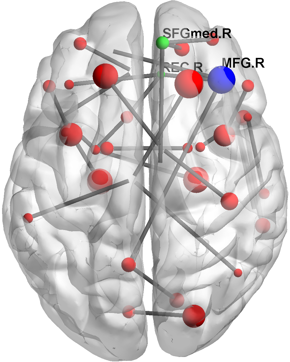
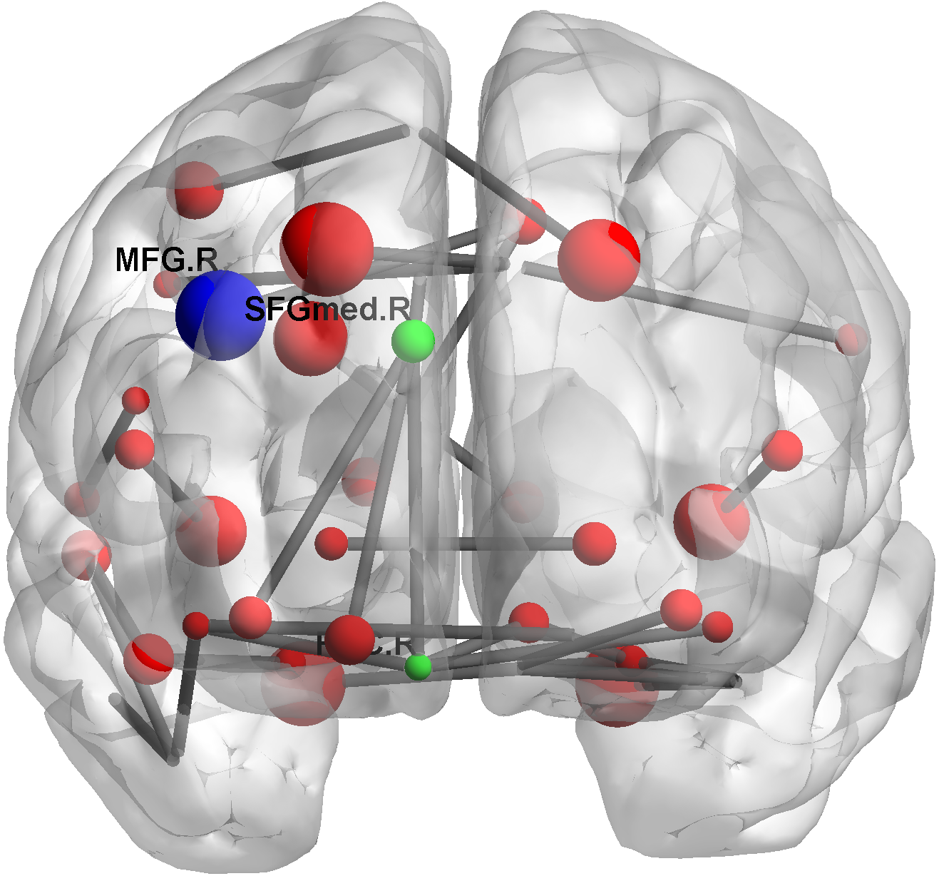
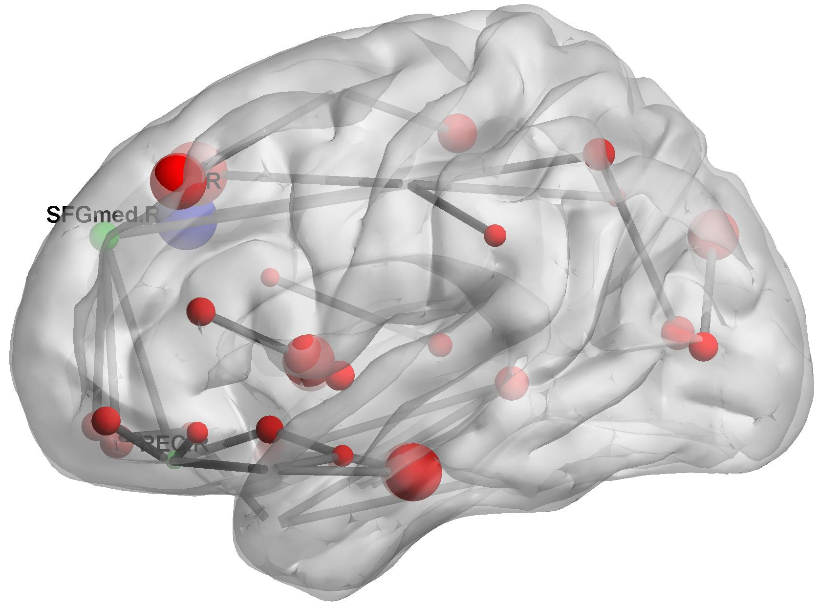
Health Control Brain Network

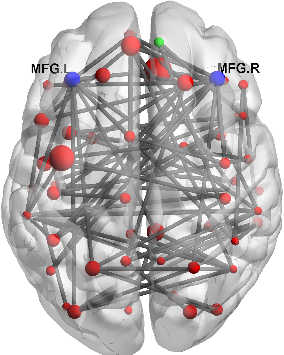
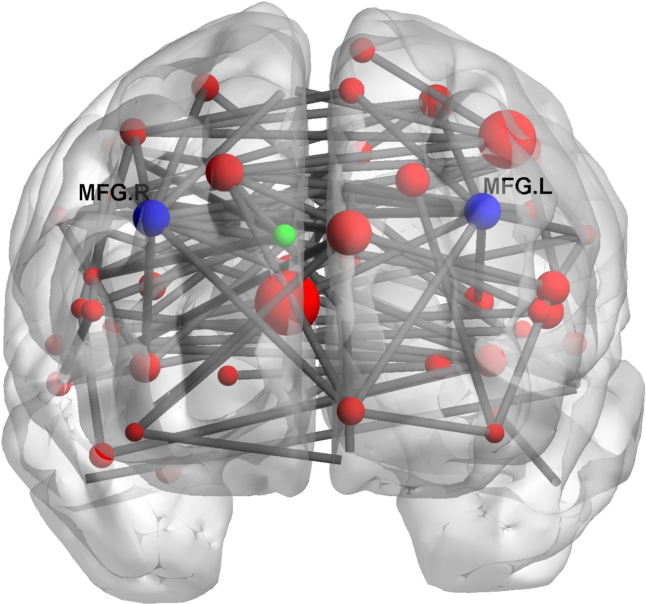
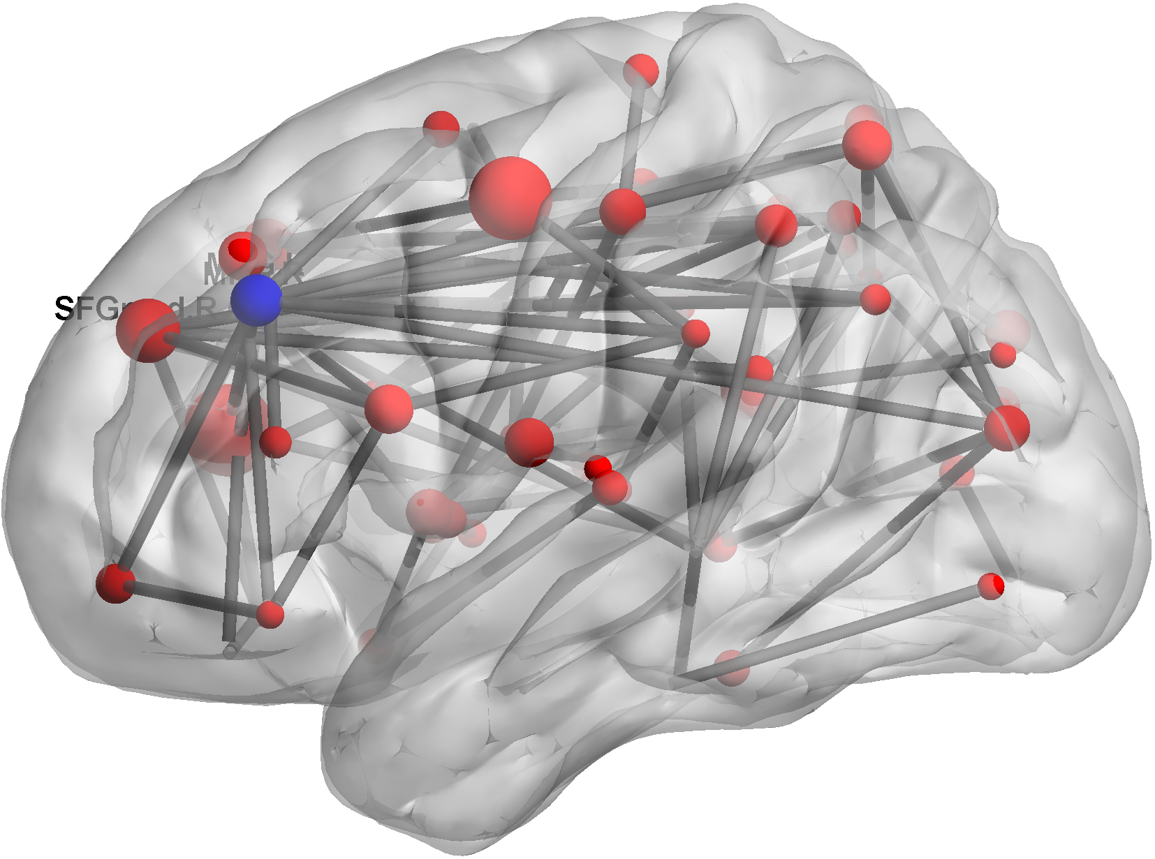
Figure 1: Identified region-level resting state brain networks for ASD patient group and health control group

8 Discussion

In additional to this, the novel contributions of our work include: 1) we propose a new framework to identify the functional brain network using formal statistical testing procedures, which make full use of the massive voxel-level brain signals and incorporate the brain anatomy into the analysis, producing neurologically more meaningful interpretations. 2) we establish the statistical theory of the proposed testing procedures, which provides the solid foundation for making valid inference on the functional brain network. 3) the proposed method is computationally very efficient and can be paralleled to achieve fast computing performance. 4) Although the development of our proposed approach is motivated by the analysis of brain imaging data, it is a general method for network construction and can be readily applied to other problems, such as identification of gene networks and social networks.

Supplementary Material

The supplementary material includes the proof of and all technical lemmas, and the simulated network (Figure 1) on 90 regions using Erd̈os-Rényi model discussed in Section 6.2.

Proof of Main Theorems

Without loss of generality, in this section, we assume $\textsf{E}(X_{k,s,i})=\textsf{E}(X_{k,t,j})=0$, and $\textsf{Var}(X_{k,s,i})=\textsf{Var}(X_{k,t,j})=1$ unless otherwise stated. Due to the space limit, we list the proofs of some theorems (Theorem 2, Theorem 4, Theorem 5, Proposition 3 and Proposition 4) here. Theorem 6 follows similar arguments of Theorem 2, and Theorem 7 follows that of Theorem 4. The proof of Theorem 1 is relatively long and the main techniques follows the proof of Theorem 1 in Cai et al. (2013), and thus is placed in the supplementary material.

In addition, to simplify the notation in the proof, we denote by $d_{st}=q_{s}q_{t}$ the total number of entries in the covariance matrix $\boldsymbol{\Upsilon}_{st}$. And also define $c(d_{st},\alpha)=2\log(d_{st})-\log\log(d_{st})+q_{\alpha}$, where $q_{\alpha}$ is the $(1-\alpha)$th quantile of null distribution $F(x)$.

To prove Theorem 2, we need Lemma 1 and Lemma 2.

Lemma 1.

Recall that $\theta_{1,st,ij}=\sigma_{ss,ii}\sigma_{tt,jj}$ and $\hat{\theta}_{1,st,ij}=\hat{\sigma}_{ss,ii}\hat{\sigma}_{tt,jj}$. Under the conditions of (C1.2) or (C1.2*) and the null $\,\mathrm{H}_{0,st}$, there exists some constant $C>0$, such that as $n,q_{0}\rightarrow\infty$,

$$\textsf{P}\left\{\max_{i,j}\left\lvert 1-\frac{\hat{\theta}_{1,st,ij}}{\theta_{1,st,ij}}\right\rvert\geq C\frac{1}{(\log q_{0})^{2}}\right\}=O(q_{0}^{-1}+n^{-\epsilon/4}).$$ (A.1)

Lemma 2.

Recall that $\theta_{st,ij}=\textsf{Var}\{(X_{k,s,i}-\mu_{s,i})(X_{k,t,j}-\mu_{t,j})\}$. Under the conditions of (C1.2) or (C1.2*), we have for some constant $C>0$ that

$$\textsf{P}\left\{\max_{(i,j)\in\mathcal{A}}\frac{(\tilde{\sigma}_{st,ij}-\sigma_{st,ij})^{2}}{\theta_{st,ij}/n}\geq x^{2}\right\}\leq C\lvert\mathcal{A}\rvert(1-\Phi(x))+O(q_{0}^{-M}+n^{-\epsilon/8})$$ (A.2)

uniformly for $0\leq x\leq(8\log q_{0})^{1/2}$ and $\mathcal{A}\subseteq\{(i,j):1\leq i\leq q_{s},1\leq j\leq q_{t}\}$. Under $\,\mathrm{H}_{0,st}$, (A.2) also holds when substituting $\theta_{st,ij}$ to $\theta_{1,st,ij}$.

Proof of Theorem 2.

Define

$$T_{st,2}=\max_{i,j}\frac{n\hat{\sigma}^{2}_{st,ij}}{\theta_{1,st,ij}}, \quad T_{st,3}=\max_{i,j}\frac{n\sigma^{2}_{st,ij}}{\theta_{1,st,ij}},$$

$$T_{st,4}=\max_{ij}\frac{n(\hat{\sigma}_{st,ij}-\sigma_{st,ij})^{2}}{\theta_{1,st,ij}}, \quad T_{st,5}=\max_{ij}\frac{n(\hat{\sigma}_{st,ij}-\sigma_{st,ij})^{2}}{\theta_{st,ij}}.$$

By Lemma 1,

$$\textsf{P}(T_{st}^{1}>q_{\alpha})\geq\textsf{P}\{T_{st,2}\geq c(d_{st},\alpha)(1+o(1))\}.$$

Since $T_{st,3}\leq 2T_{st,4}+2T_{st,2}$ and $T_{st,3}\geq 4(1+\kappa_{1})\log d_{st}$,

$$\ \textsf{P}\{T_{st,2}\geq c(d_{st},\alpha)(1+o(1))\}$$

$$\geq \ \textsf{P}\{T_{st,3}-2T_{st,4}\geq 2c(d_{st},\alpha)(1+o(1))\}$$

$$= \ \textsf{P}\{T_{st,4}\leq T_{st,3}/2-c(d_{st},\alpha)(1+o(1))\}$$

$$= \ \textsf{P}\{T_{st,4}\leq(2\kappa_{1}\log d_{st}+\log\log_{dst}-q_{\alpha})(1-o(1))\}.$$

By Condition (1.3), $T_{st,5}\geq T_{st,4}/\kappa_{1}$. It follows that

$$\textsf{P}\{T_{st,4}\leq(2\kappa_{1}\log d_{st}+\log\log_{dst}-q_{\alpha})(1+o(1))\}\\ \geq\textsf{P}\{T_{st,5}\leq(2\log d_{st}+(1/\kappa_{1})\log\log d_{st}-(1/\kappa_{1})q_{\alpha})(1-o(1))\}.$$

By Lemma 2,

$$\textsf{P}\{T_{st,5}\leq(2\log d_{st}+(1/\kappa_{1})\log\log d_{st}-(1/\kappa_{1})q_{\alpha})(1-o(1))\}\rightarrow 1.$$

∎

Proof of Theorem 4.

It suffices to show the results for normal distribution which satisfies (C2) and (C2*). Denote $\min(q_{s},q_{t})=q^{\ast}(s,t)$. Let $\mathcal{M}(s,t)=\{\mathcal{S}:\ \mathcal{S}\subseteq\{1,\ldots,q^{\ast}\},\ \textsf{Card}(\mathcal{S})=r_{st}\}$ denote the set of all the subsets of $\{1,\ldots,q^{\ast}\}$ with cardinality $r_{st}$. Let $\hat{m}$ be a random subset of $\{1,\ldots,q^{\ast}\}$, which is uniformly distributed on $\mathcal{M}$. Consider such covariance matrix of $(\boldsymbol{X}_{s},\boldsymbol{X}_{t})^{\mathrm{\scriptscriptstyle T}}$:

$$\boldsymbol{\Sigma}_{\hat{m}}^{\ast}=\begin{pmatrix}\mathbf{I}_{q_{s}\times q_{s}}&\boldsymbol{\Sigma}_{st,\hat{m}}^{\ast}\\ \boldsymbol{\Sigma}_{st,\hat{m}}^{\ast\mathrm{\scriptscriptstyle T}}&\mathbf{I}_{q_{t}\times q_{t}}\end{pmatrix},\quad\text{ and }\boldsymbol{\Sigma}_{st,\hat{m}}^{\ast}=(\sigma_{st,ij})_{q_{s}\times q_{t}},$$

with

$$\sigma_{st,i_{1}i_{1}}=\rho=c(\log d_{st}/n)^{1/2},\ \sigma_{st,i_{2}i_{2}}=\sigma_{st,ij}=0\quad(i_{1}\in\mathcal{M}(s,t),\ i_{2}\in\mathcal{M}(s,t)^{c},\ j\neq i).$$

Here $c$ is a positive constant which will be specified later. Without loss of generality, suppose $q_{s}\leq q_{t}$. Let’s reorder the variables $\boldsymbol{X}=(X_{s,1},X_{t,1},\ldots,X_{s,q_{s}},X_{t,q_{s}},\ldots,X_{t,q_{t}})^{\mathrm{\scriptscriptstyle T}}$. Then the covariance matrix of $\boldsymbol{X}$ is $\boldsymbol{\Sigma}_{\hat{m}}=\textsf{diag}(A(i),\ldots,A(i),\mathbf{I}_{q_{t}-q_{s}})$, with

$$A(i)=\begin{pmatrix}1&\rho\\ \rho&1\end{pmatrix}\text{ if }i\in\hat{m};\quad\text{and }A(i)=\mathbf{I}_{2}\text{ if }i\in\hat{m}^{c}.$$

It is easy to see that the precision matrix is $\boldsymbol{\Omega}_{\hat{m}}=\textsf{diag}(B(i),\ldots,B(i),\mathbf{I}_{q_{t}-q_{s}})$, with

$$A(i)=\frac{1}{1-\rho^{2}}\begin{pmatrix}1&-\rho\\ -\rho&1\end{pmatrix}\text{ if }i\in\hat{m};\quad\text{and }A(i)=\mathbf{I}_{2}\text{ if }i\in\hat{m}^{c}.$$

We construct a class of $\boldsymbol{\Sigma}$: $\mathcal{Q}=\{\boldsymbol{\Sigma}_{\hat{m}},\hat{m}\in\mathcal{M}(s,t)\}$. Let $\boldsymbol{\Sigma}_{0}=\mathbf{I}$, and $\boldsymbol{\Sigma}_{1}$ be uniformly distributed on $\mathcal{Q}$. Let $\mu_{\rho}$ be the distribution of $\boldsymbol{\Sigma}_{1}$. It is a measure on $\{\Delta\in\mathcal{S}(r_{st},s,t):\ \lVert\Delta\rVert_{F}^{2}=r_{st}\rho^{2}\}$. Let $dP_{a}(\boldsymbol{X})$ be the likelihood function given $\boldsymbol{\Sigma}_{a}$, $a=0,1$. Define

$$L_{\mu_{\rho}}(\boldsymbol{X})=\textsf{E}_{\mu_{\rho}}\left\{\frac{dP_{1}(\boldsymbol{X})}{dP_{0}(\boldsymbol{X})}\right\},$$

where $\textsf{E}_{\mu_{\rho}}$ is the expectation on $\boldsymbol{\Sigma}_{\hat{m}}$. By the arguments in Section 7.1 in Baraud (2002), it suffices to show that $\textsf{E}_{0}(L_{\mu_{\rho}}^{2})\leq 1+o(1)$.

We have

$$L_{\mu_{\rho}}=\textsf{E}_{\hat{m}}\left[\prod_{k=1}^{n}\frac{1}{\lvert\boldsymbol{\Sigma}_{\hat{m}}\rvert^{1/2}}\exp\left\{-\frac{1}{2}\boldsymbol{X}_{k}^{\mathrm{\scriptscriptstyle T}}(\boldsymbol{\Omega}_{\hat{m}}-\mathbf{I})\boldsymbol{X}_{k}\right\}\right]$$

Let $E_{0}$ be the expectation on $\boldsymbol{X}_{k}$ with $\mathrm{N}(0,\mathbf{I})$ distribution. Then

$$\textsf{E}_{0}(L^{2}_{\mu_{\rho}}) =\textsf{E}_{0}\left[\frac{1}{{q^{\ast}\choose r_{st}}}\sum_{m\in\mathcal{M}}\left\{\prod_{k=1}^{n}\frac{1}{\lvert\boldsymbol{\Sigma}_{m}\rvert^{1/2}}\exp\left(-\frac{1}{2}\boldsymbol{X}_{k}^{\mathrm{\scriptscriptstyle T}}(\boldsymbol{\Omega}_{m}-\mathbf{I})\boldsymbol{X}_{k}\right)\right\}\right]^{2}$$

$$=\frac{1}{{q^{\ast}\choose r_{st}}^{2}}\sum_{m,m^{\prime}\in\mathcal{M}}\textsf{E}_{0}\left[\prod_{k=1}^{n}\frac{1}{\lvert\boldsymbol{\Sigma}_{m}\rvert^{1/2}}\frac{1}{\lvert\boldsymbol{\Sigma}_{m^{\prime}}\rvert^{1/2}}\exp\left\{-\frac{1}{2}\boldsymbol{X}_{k}^{\mathrm{\scriptscriptstyle T}}(\boldsymbol{\Omega}_{m}+\boldsymbol{\Omega}_{m^{\prime}}-2\mathbf{I})\boldsymbol{X}_{k}\right\}\right]$$

Set $\boldsymbol{\Omega}_{m}+\boldsymbol{\Omega}_{m^{\prime}}-2\mathbf{I}=(a_{s_{1},s_{2},i,j})$, $s_{1},s_{2}\in\{s,t\}$, $i=1,\ldots,q_{s_{1}}$, and $j=1,\ldots,q_{s_{2}}$. If $i\in m\cap m^{\prime}$, $a_{ss,ii}=a_{tt,ii}=2\rho^{2}/(1-\rho^{2})$, $a_{st,ii}=-2\rho/(1-\rho^{2})$. If $i\in m\Delta m^{\prime}$, $a_{ss,ii}=a_{tt,ii}=1/(1-\rho^{2})-1$, $a_{st,ii}=-\rho/(1-\rho^{2})$. Otherwise, $a_{s_{1},s_{2},i,j}=0$. Now let $t=\lvert m\cap m^{\prime}\rvert$. By simple calculations, we have

$$\textsf{E}_{0}(L_{\mu_{\rho}}^{2}) =\frac{1}{{q^{\ast}\choose r_{st}}^{2}}(1-\rho^{2})^{-nr_{st}}\sum_{t=0}^{r_{st}}{q^{\ast}\choose r_{st}}{r_{st}\choose t}{q^{\ast}-r_{st}\choose r_{st}-t}1^{tn}(1-\rho^{2})^{(2r_{st}-t)n/2}$$

$$={q^{\ast}\choose r_{st}}^{-1}\sum_{t=1}^{r_{st}}{r_{st}\choose t}{q^{\ast}-r_{st}\choose r_{st}-t}(1-\rho^{2})^{-tn/2}$$

$$\leq q^{\ast r_{st}}\frac{(q^{\ast}-r_{st})!}{q^{\ast}!}\sum_{t=0}^{r_{st}}{r_{st}\choose t}\left(\frac{s}{q^{\ast}}\right)^{t}\left(\frac{1}{1-\rho^{2}}\right)^{tn/2}$$

$$=(1+o(1))\left(1+\frac{r_{st}}{q^{\ast}(1-\rho^{2})^{n/2}}\right)^{r_{st}}$$

$$\leq\exp\{r_{st}\log(1+r_{st}q^{\ast c^{2}-1})\}(1+o(1))$$

$$\leq\exp(r_{st}^{2}q^{\ast c^{2}-1})(1+o(1))$$

For sufficiently small $c^{2}$, $\textsf{E}_{0}(L_{\mu_{\rho}}^{2})=1+o(1)$, and the theorem is proved. ∎

Proof of Theorem 5.

Define

$$T_{st}=n\max_{ij}\rho_{\varepsilon,st}, \quad\hat{T}_{st}=\max_{i,j}\frac{n(\hat{\sigma}_{\varepsilon,st,ij}-\sigma_{\varepsilon,st,ij})^{2}}{\theta_{\varepsilon,st,ij}}$$

$$\tilde{T}_{st}=\max_{ij}\frac{n(\tilde{\sigma}_{\varepsilon,st,ij}-\sigma_{\varepsilon,st,ij})^{2}}{\theta_{\varepsilon,st,ij}}, \quad\breve{T}_{st}=\max_{i,j}\frac{n(\breve{\sigma}_{\varepsilon,st,ij}-\sigma_{\varepsilon,st,ij})^{2}}{\theta_{\varepsilon,st,ij}},$$

where

$$\hat{\sigma}_{\varepsilon,st,ij}=\sum_{k=1}^{n}\hat{\varepsilon}_{k,s,i}\hat{\varepsilon}_{k,t,j}/n,\quad\tilde{\sigma}_{\varepsilon,st,ij}=\sum_{k=1}^{n}\tilde{\varepsilon}_{k,s,i}\tilde{\varepsilon}_{k,t,j}/n,\quad\breve{\sigma}_{\varepsilon,st,,ij}=\sum_{k=1}^{n}\varepsilon_{k,s,i}\varepsilon_{k,t,j}/n.$$

By Condition (2.3) and $\max_{i}\lvert\tilde{\sigma}_{\varepsilon,ss,ii}-\sigma_{\varepsilon,ss,ii}\rvert=O_{P}\{(\log q_{0})^{-1-\alpha_{0}}\}$,

$$\lvert\hat{\theta}_{\varepsilon,st,ij}-\theta_{\varepsilon,st,ij}\rvert\leq\lvert\hat{\sigma}_{\varepsilon,ss,ii}\hat{\sigma}_{\varepsilon,tt,jj}-\sigma_{\varepsilon,ss,ii}\sigma_{\varepsilon,tt,jj}\rvert\\ \leq O_{P}\left\{\max(\lvert\hat{\sigma}_{\varepsilon,ss,ii}-\sigma_{\varepsilon,ss,ii}\rvert,\lvert\hat{\sigma}_{\varepsilon,tt,jj}-\sigma_{\varepsilon,tt,jj}\rvert)\right\}=O_{P}\{(\log q_{0})^{-1-\alpha_{0}}\}.$$

By (C2.2), $\theta_{\varepsilon,st,ij}\geq 1/c_{0}^{2}$. Thus with proability tending to one,

$$\lvert T_{st}-\hat{T}_{st}\rvert \leq C\hat{T}_{st}(\log q_{0})^{-1-\alpha_{0}}$$

$$\lvert\hat{T}_{st}-\tilde{T}_{st}\rvert \leq C(\log q_{0})^{-1-\alpha_{0}}$$

$$\lvert\breve{T}_{st}-\tilde{T}_{st}\rvert \leq Cn(\max_{1\leq i\leq q_{s}}\bar{\varepsilon}_{s,i}^{4}+\max_{1\leq j\leq q_{t}}\bar{\varepsilon}_{t,j}^{4})+Cn^{1/2}\breve{T}_{st}^{1/2}(\max_{1\leq i\leq q_{s}}\bar{\varepsilon}_{s,i}^{2}+\max_{1\leq j\leq q_{t}}\bar{\varepsilon}_{t,j}^{2}).$$

The second inequality above is by Condition (C2.3). Note that

$$\max_{1\leq i\leq q_{s}}\lvert\bar{\varepsilon}_{s,i}\rvert+\max_{1\leq t\leq q_{t}}\lvert\bar{\varepsilon}_{t,j}\rvert=O_{P}((\log q_{0}/n)^{1/2}),$$

Thus, it suffices to show that for any $x\in\mathbb{R}$,

$$\textsf{P}\{\breve{T}_{st}\leq 2\log d_{st}-2\log\log(d_{st})+x\}\rightarrow exp\left\{-\frac{1}{\pi^{1/2}}\exp\left(-\frac{x}{2}\right)\right\}.$$

The rest of the proof is similar to the proof of Theorem 1. ∎

Proof of Proposition 3.

We first decompose $\hat{\sigma}_{\varepsilon,st,ij}$ as follows:

$$\frac{1}{n}\sum_{k=1}^{n}\hat{\varepsilon}_{k,s,i}\hat{\varepsilon}_{k,t,j}=\frac{1}{n}\sum_{k=1}^{n}\tilde{\varepsilon}_{k,s,i}\tilde{\varepsilon}_{k,t,j}-A_{1,s,t,i,j}-A_{2,s,t,i,j}+A_{3,s,t,i,j},$$

where

$$A_{1,s,t,i,j} =\frac{1}{n}\sum_{k=1}^{n}\tilde{\varepsilon}_{k,s,i}(\boldsymbol{X}_{k,t,-j}-\bar{\boldsymbol{X}}_{t,-j})^{\mathrm{\scriptscriptstyle T}}(\hat{\boldsymbol{\beta}}_{t,j}-\boldsymbol{\beta}_{t,j})$$

$$A_{2,s,t,i,j} =\frac{1}{n}\sum_{k=1}^{n}\tilde{\varepsilon}_{k,t,j}(\boldsymbol{X}_{k,s,-i}-\bar{\boldsymbol{X}}_{s,-i})^{\mathrm{\scriptscriptstyle T}}(\hat{\boldsymbol{\beta}}_{s,i}-\boldsymbol{\beta}_{s,i})$$

$$A_{3,s,t,i,j} =(\hat{\boldsymbol{\beta}}_{s,i}-\boldsymbol{\beta}_{s,i})^{\mathrm{\scriptscriptstyle T}}\hat{\boldsymbol{\Sigma}}_{st,-i,-j}(\hat{\boldsymbol{\beta}}_{t,j}-\boldsymbol{\beta}_{t,j})$$

We bound each term in order.

Note that for all $s,t\in\{1,\ldots,p\}$,

$$\lvert A_{1,s,t,i,j}\rvert\leq \left|\frac{1}{n}\sum_{k=1}^{n}\tilde{\epsilon}_{k,s,i}(\boldsymbol{X}_{k,t,-j}-\bar{\boldsymbol{X}}_{k,t,-j})-\textsf{Cov}(\tilde{\varepsilon}_{k,s,i},\boldsymbol{X}_{k,t,-j})\right\rvert_{\infty}\left\lvert\hat{\boldsymbol{\beta}}_{t,j}-\beta_{t,j}\right\rvert_{1}$$

$$\phantom{a}+\left\lvert\textsf{Cov}(\tilde{\varepsilon}_{k,s,i},\boldsymbol{X}_{k,s,-j}^{\mathrm{\scriptscriptstyle T}})\right(\hat{\boldsymbol{\beta}}_{t,j}-\boldsymbol{\beta}_{t,j})\rvert.$$ (A.3)

And also for any $M>0$, there exists sufficiently large $C>0$ such that

$$\textsf{P}\left\{\max_{1\leq i\leq q_{s},1\leq j\leq q_{t}}\left\lvert\frac{1}{n}\sum_{k=1}^{n}\tilde{\varepsilon}_{k,s,i}(X_{k,t,-j}-\bar{X}_{t,-j})-\textsf{Cov}(\tilde{\varepsilon}_{k,s,i},\boldsymbol{X}_{k,t,-j})\right\rvert_{\infty}\geq C(\log d_{st}/n)^{1/2}\right\}=O(q_{0}^{-M}).$$

Recall the definition of $a_{v,1}$ and $a_{v,2}$ in (13).

When $s=t$ and $i=j$, $\textsf{Cov}(\tilde{\varepsilon}_{k,s,i},\boldsymbol{X}_{k,s,-i})=\boldsymbol{0}$. Therefore

$$\max_{1\leq i\leq q_{s}}\left\lvert A_{1,s,s,i,i}\right\rvert=O_{P}\left\{a_{s,1}(\log q_{s}/n)^{1/2}\right\}.$$

When $s\neq t$, under $\,\mathrm{H}_{0,st}$, $\textsf{Cov}(\tilde{\varepsilon}_{k,s,i},\boldsymbol{X}_{k,t,-j})=\boldsymbol{0}$. Therefore

$$\max_{1\leq i\leq q_{s},1\leq j\leq q_{t}}\left\lvert A_{1,s,t,i,j}\right\rvert=O_{P}\left\{a_{t,1}(\log d_{st}/n)^{1/2}\right\}.$$

When $s\neq t$ and under $\,\mathrm{H}_{1,st}$,

$$\left\lvert\textsf{Cov}(\tilde{\varepsilon}_{k,s,i},\boldsymbol{X}_{k,s,-j}^{\mathrm{\scriptscriptstyle T}})\right(\hat{\boldsymbol{\beta}}_{t,j}-\boldsymbol{\beta}_{t,j})\rvert \leq\left\{\textsf{Var}(\tilde{\varepsilon}_{k,s,i})\right\}^{1/2}\left\{(\hat{\boldsymbol{\beta}}_{t,j}-\boldsymbol{\beta}_{t,j})^{\mathrm{\scriptscriptstyle T}}\boldsymbol{\Sigma}_{tt,-j,-j}(\hat{\boldsymbol{\beta}}_{t,j}-\boldsymbol{\beta}_{t,j})\right\}^{1/2}$$

$$\leq c_{0}a_{t,2}$$

Therefore,

$$\max_{1\leq i\leq q_{s},1\leq j\leq q_{t}}\left\lvert A_{1,s,t,i,j}\right\rvert=O_{P}\left[a_{t,1}(\log d_{st}/n)^{1/2}+a_{t,2}\right]$$

We can show bounds for $A_{2,s,t,i,j}$ similarly.

Next, we bound $A_{3,s,t,i,j}$.

$$A_{3,s,t,i,j}= (\hat{\boldsymbol{\beta}}_{k,s,i}-\boldsymbol{\beta}_{k,s,i})^{\mathrm{\scriptscriptstyle T}}(\hat{\boldsymbol{\Sigma}}_{st,-i,-j}-\boldsymbol{\Sigma}_{st,-i,-j})(\hat{\boldsymbol{\beta}}_{k,t,j}-\boldsymbol{\beta}_{k,t,j})$$

$$+(\hat{\boldsymbol{\beta}}_{k,s,i}-\boldsymbol{\beta}_{k,s,i})^{\mathrm{\scriptscriptstyle T}}\boldsymbol{\Sigma}_{st,-i,-j}(\hat{\boldsymbol{\beta}}_{k,t,j}-\boldsymbol{\beta}_{k,t,j})$$

It is easy to show that for any $M>0$, there exists sufficiently large $C>0$ such that

$$\textsf{P}\left\{\max_{1\leq i\leq q_{s},1\leq j\leq q_{t}}\lvert\hat{\sigma}_{st,ij}-\sigma_{st,ij}\rvert\geq C(\log d_{st}/n)^{1/2}\right\}=O(q_{0}^{-M}).$$

When $s\neq t$, under $\,\mathrm{H}_{0,st}$, $\boldsymbol{\Sigma}_{st,-i,-j}=\boldsymbol{0}$; and under $\,\mathrm{H}_{1,st}$, $\lVert\boldsymbol{\Sigma}_{st,-i,-j}\rVert_{2}\leq c_{0}$. By the inequality

$$\left\lvert(\hat{\boldsymbol{\beta}}_{k,s,i}-\boldsymbol{\beta}_{k,s,i})^{\mathrm{\scriptscriptstyle T}}(\hat{\boldsymbol{\Sigma}}_{st,-i,-j}-\boldsymbol{\Sigma}_{st,-i,-j})(\hat{\boldsymbol{\beta}}_{k,t,j}-\boldsymbol{\beta}_{k,t,j})\right\rvert\\ \leq\left\lvert\hat{\boldsymbol{\Sigma}}_{st,-i,-j}-\boldsymbol{\Sigma}_{st,-i,-j}\right\rvert_{\infty}\lvert\hat{\boldsymbol{\beta}}_{k,s,i}-\boldsymbol{\beta}_{k,s,i}\rvert_{1}\lvert\hat{\boldsymbol{\beta}}_{k,t,j}-\boldsymbol{\beta}_{k,t,j}\rvert_{1},$$ (A.4)

we have under $\,\mathrm{H}_{0,st}$,

$$\max_{1\leq i\leq q_{s},1\leq j\leq q_{t}}\left\lvert A_{3,s,t,i,j}\right\rvert=O_{P}\left\{a_{s,1}a_{t,1}(\log d_{st}/n)^{1/2}\right\};$$

and under $\,\mathrm{H}_{1,st}$,

$$\max_{1\leq i\leq q_{s},1\leq j\leq q_{t}}\left\lvert A_{3,s,t,i,j}\right\rvert=O_{P}\left\{a_{s,1}a_{t,1}(\log d_{st}/n)^{1/2}+a_{s,2}a_{t,2}\right\}.$$

When $s=t$, we can show by similar argument that under $\,\mathrm{H}_{0,st}$,

$$\max_{1\leq i\leq q_{s},1\leq j\leq q_{t}}\lvert A_{3,s,s,i,j}\rvert=O_{P}\left\{a_{s,1}^{2}(\log q_{s}/n)^{1/2}\right\};$$

and under $\,\mathrm{H}_{1,st}$,

$$\max_{1\leq i\leq q_{s},1\leq j\leq q_{t}}\lvert A_{3,s,s,i,j}\rvert=O_{P}\left\{a_{s,1}^{2}(\log q_{s}/n)^{1/2}+a_{s,2}^{2}\right\}.$$

Therefore, when $s\neq t$, under $\,\mathrm{H}_{0,st}$

$$\frac{1}{n}\sum_{k=1}^{n}\hat{\varepsilon}_{k,s,i}\hat{\varepsilon}_{k,t,j}=\frac{1}{n}\sum_{k=1}^{n}\tilde{\varepsilon}_{k,s,i}\tilde{\varepsilon}_{k,t,j}+O_{P}\left\{(a_{s,1}a_{t,1}+a_{s,1}+a_{t,1})\left(\frac{\log d_{st}}{n}\right)^{1/2}\right\};$$ (A.5)

and under $\,\mathrm{H}_{1,st}$,

$$\frac{1}{n}\sum_{k=1}^{n}\hat{\varepsilon}_{k,s,i}\hat{\varepsilon}_{k,t,j}=\frac{1}{n}\sum_{k=1}^{n}\tilde{\varepsilon}_{k,s,i}\tilde{\varepsilon}_{k,t,j}+O_{P}\left\{(a_{s,1}a_{t,1}+a_{s,1}+a_{t,1})\left(\frac{\log d_{st}}{n}\right)^{1/2}+(a_{s,2}a_{t,2}+a_{s,2}+a_{t,2})\right\}.$$ (A.6)

When $s=t$ and $i=j$, under $\,\mathrm{H}_{0,st}$,

$$\frac{1}{n}\sum_{k=1}^{n}\hat{\varepsilon}_{k,s,i}^{2}=\frac{1}{n}\sum_{k=1}^{n}\tilde{\varepsilon}_{k,s,i}^{2}+O_{P}\left\{(a_{s,1}^{2}+a_{s,1})\left(\frac{\log q_{s}}{n}\right)^{1/2}\right\};$$ (A.7)

and under $\,\mathrm{H}_{1,st}$,

$$\frac{1}{n}\sum_{k=1}^{n}\hat{\varepsilon}_{k,s,i}^{2}=\frac{1}{n}\sum_{k=1}^{n}\tilde{\varepsilon}_{k,s,i}^{2}+O_{P}\left\{(a_{s,1}^{2}+a_{s,1})\left(\frac{\log q_{s}}{n}\right)^{1/2}+a_{s,2}^{2}\right\}.$$ (A.8)

It then suffices to show that for $v=1,\ldots,p$, $a_{v,2}=O_{P}\{(\log q_{0})^{-1-\alpha_{0}}\}$ and $a_{v,1}=O_{P}\{n(\log q_{0})^{-2-\alpha_{0}}\}$.

By the proof of Proposition 4.1 in Liu (2013), page 2975, with probability tending to 1,

$$\lvert\mathbf{D}_{v,i}^{-1/2}\hat{\boldsymbol{\Sigma}}_{vv,-i,-i}\hat{\boldsymbol{\beta}}_{v,i}-\mathbf{D}_{v,i}^{-1/2}\mathbf{b}_{v,i}\rvert_{\infty}\leq\lambda_{v,i}(2).$$

And it follows that

$$\lvert\mathbf{D}_{v,i}^{-1/2}\hat{\boldsymbol{\Sigma}}_{vv,-i,-i}(\hat{\boldsymbol{\beta}}_{v,i}-\boldsymbol{\beta}_{v,i})\rvert_{\infty}\leq 2\lambda_{v,i}(2).$$

And also by

$$\max_{1\leq i\leq q_{v}}\lvert\boldsymbol{\beta}_{v,i}\rvert_{0}=o\left\{\lambda_{\min}(\boldsymbol{\Sigma})(n/\log q_{0})^{1/2}\right\}$$

and the inequality

$$\boldsymbol{\delta}^{\mathrm{\scriptscriptstyle T}}\hat{\boldsymbol{\Sigma}}_{vv,-i,-i}\boldsymbol{\delta}\geq\lambda_{\min}(\boldsymbol{\Sigma}_{-i,-i})\lvert\boldsymbol{\delta}\rvert_{2}^{2}-O_{P}\{(\log q_{0}/n)^{1/2}\}\lvert\boldsymbol{\delta}\rvert_{1},$$

we can see that the restricted eigenvalue assumption RE$(s,s,1)$ in Bickel et al. (2009), page 1711, holds with $\kappa(s,s,1)\geq c\lambda_{\min}(\boldsymbol{\Sigma})^{1/2}$. And by the proof of Theorem 7.1 in Bickel et al. (2009),

$$a_{v,1}=O_{P}\left\{\max_{1\leq i\leq q_{v}}\lvert\boldsymbol{\beta}_{v,i}\rvert_{0}(\log q_{v}/n)^{1/2}\right\},\quad a_{v,2}=O_{P}\left[\left\{\max_{1\leq i\leq q_{v}}\lvert\boldsymbol{\beta}_{v,i}\rvert_{0}(\log q_{n}/n)\right\}^{1/2}\{\lambda_{\min}(\boldsymbol{\Sigma})\}^{-1}\right]$$

∎

Proof of Proposition 4.

By Proof of Proposition 4.2 in Liu (2013), we have with probability tending to one,

$$\lvert\mathbf{D}_{v,i}^{-1/2}\hat{\boldsymbol{\Sigma}}_{vv,-i,-i}\mathbf{D}_{v,i}^{-1/2}(\hat{\boldsymbol{\alpha}}_{v,i}-\mathbf{D}_{v,i}^{1/2}\boldsymbol{\beta}_{v,i})\rvert_{\infty}\leq 2\lambda_{v,i}(\delta).$$

Then by (A.5), (A.6), (A.7), (A.8), and the proof of Theorem 7.2 in Bickel et al. (2009), we get Condition (2.3) holds for $\boldsymbol{\beta}_{v,i}(\delta)$ with $\delta>2$. ∎

Supplementary Material for “High Dimensional Tests for Functional Brain Networks”

S.1 Proof of Other Theorems

Lemma 3.

For any fixed integer $D\geq 1$ and real number $x\in\mathbb{R}$,

$$\sum_{1\leq k_{1}<\ldots<k_{D}\leq K}\textsf{P}\left(\lvert\mathbf{N}_{D}\rvert_{\min}\geq y(d_{st},x)^{1/2}\pm\epsilon_{n}(\log q_{0})^{-1/2}\right)=\frac{1}{D!}\left\{\frac{1}{\sqrt{\pi}}\exp\left(-\frac{x}{2}\right)\right\}^{D}(1+o(1)).$$

Proof of Theorem 1.

Without loss of generality, we assume that $\mu_{s,i}=\mu_{t,j}=0$, $\sigma_{ss,ii}=\sigma_{tt,jj}=1$, for $i=1,\ldots,q_{s}$, and $j=1,\ldots,q_{t}$. To simplify notation, let $T=n\cdot\max_{ij}\hat{\rho}_{st,ij}$.

Define

$$\hat{T}=\max_{i,j}\frac{(\hat{\sigma}_{st,ij}-\sigma_{st,ij})^{2}}{\theta_{st,ij}/n},\quad\text{and }\tilde{T}=\max_{i,j}\frac{(\tilde{\sigma}_{st,ij}-\sigma_{st,ij})^{2}}{\theta_{st,ij}/n}$$

By Lemma 1, with probability at least $1-O(q_{0}^{-1}+n^{-\epsilon/8})$,

$$\lvert T-\hat{T}\rvert \leq C\hat{T}\frac{1}{(\log q_{0})^{2}}$$

$$\lvert\hat{T}-\tilde{T}\rvert \leq\max_{ij}\left\lvert\frac{(\hat{\sigma}_{st,ij}-\tilde{\sigma}_{st,ij})(\hat{\sigma}_{st,ij}+\tilde{\sigma}_{st,ij}-2\sigma_{st,ij})}{\theta_{st,ij}/n}\right\rvert$$

$$\leq\max_{ij}\left\lvert\frac{(\bar{X}_{s,i}\bar{X}_{t,j})\left(2\tilde{\sigma}_{st,ij}-2\sigma_{st,ij}-\bar{X}_{s,i}\bar{X}_{t,j}\right)}{\theta_{st,ij}/n}\right\rvert$$

$$\leq n^{1/2}\tilde{T}^{1/2}\left(\max_{i}\bar{\boldsymbol{X}}_{s,i}^{2}+\max_{j}\bar{\boldsymbol{X}}_{t,j}^{2}\right)+2n\left(\max_{i}\bar{\boldsymbol{X}}_{s,i}^{4}+\max_{j}\bar{\boldsymbol{X}}_{t,j}^{4}\right)$$

By similar arguments as (9) and (11), $\max_{i}\lvert\bar{X}_{s,i}\rvert+\max_{j}\lvert\bar{X}_{t,j}\rvert=O_{P}\left\{(\log q_{0}/n)^{1/2}\right\}$. Set $y(d_{st},x)=2\log d_{st}-\log\log d_{st}+x$. By Lemma 2, it suffices to show that for any $x\in\mathbb{R}$,

$$\textsf{P}\{\tilde{T}\leq y(d_{st},x)\}\rightarrow\exp\left\{-\frac{1}{\pi^{1/2}}\exp\left(-\frac{x}{2}\right)\right\}.$$

as $n$ and $d\rightarrow\infty$.

Let

$$\mathcal{O}_{st} =\{(i,j):\ 1\leq i\leq q_{s},1\leq j\leq q_{t}\},$$

$$\mathcal{A}_{st} =\{(i,j):i\not\in\mathcal{M}_{s},i\not\in\mathcal{D}_{s}^{(1)},j\not\in\mathcal{M}_{t},j\not\in\mathcal{D}_{t}^{(1)}\}.$$

Let

$$\tilde{T}_{\mathcal{A}_{st}}=\max_{(i,j)\in\mathcal{A}_{st}}\frac{n\tilde{\sigma}_{st,ij}^{2}}{\theta_{st,ij}},\quad\tilde{T}_{\mathcal{O}_{st}\setminus\mathcal{A}_{st}}=\max_{(i,j)\in\mathcal{O}_{st}\setminus\mathcal{A}_{st}}\frac{n\tilde{\sigma}_{st,ij}^{2}}{\theta_{st,ij}}.$$

Then

$$\lvert\textsf{P}\{\tilde{T}\geq y(d_{st},x)\}-\textsf{P}\{\tilde{T}_{\mathcal{A}_{st}}\geq y(d_{st},x)\}\rvert\leq\textsf{P}\{\tilde{T}_{\mathcal{O}_{st}\setminus\mathcal{A}_{st}}\geq y(d_{st},x)\}.$$

Note that $\textsf{Card}(\mathcal{O}_{st}\setminus\mathcal{A}_{st})=o(d_{st})$. Then by Lemma 2,

$$\textsf{P}\left\{\tilde{T}_{\mathcal{O}_{st}\setminus\mathcal{A}_{st}}\geq y(d_{st},x)\right\}\leq o(d_{st})\cdot Cd_{st}^{-1}+o(1)=o(1).$$

It suffies to show that for any $x\in\mathbb{R}$,

$$\textsf{P}\{\tilde{T}_{\mathcal{A}_{st}}\leq y(d_{st},x)\}\rightarrow\exp\left\{-\pi^{-1/2}\exp\left(-x/2\right)\right\}.$$

as $n$ and $q_{0}\rightarrow\infty$.

We arrange the indices $\{(i,j):(i,j)\in\mathcal{A}_{st}\}$ in any ordering and set them as $\{(i_{m},j_{m}):1\leq m\leq d_{1}\}$, with $d_{1}\asymp d_{st}$. Let $\theta_{st,l}=\theta_{st,i_{l}j_{l}}$. For $k=1,\ldots,n$, define

$$Z_{k,l} =X_{k,s,i_{l}}X_{k,t,j_{l}}-\sigma_{st,i_{l}j_{l}},$$

$$\hat{Z}_{k,l} =Z_{k,l}I(\lvert Z_{k,l}\rvert\leq\tau_{n})-\textsf{E}\{Z_{k,l}I(\lvert Z_{k,l}\rvert\leq\tau_{n})\},$$

$$\tilde{Z}_{k,l} =Z_{k,l}-\hat{Z}_{k,l},$$

$$V_{l} =\sum_{k=1}^{n}Z_{k,l}/(n\theta_{l})^{1/2},$$

$$\hat{V}_{l} =\sum_{k=1}^{n}\hat{Z}_{k,l}/(n\theta_{l})^{1/2},$$

$$\tilde{V}_{l} =\sum_{k=1}^{n}\tilde{Z}_{k,l}/(n\theta_{l})^{1/2},$$

where $\tau_{n}=8\eta^{-1}\log(d_{st}+n)$ if (C1.2) holds, and $\tau_{n}=n^{1/2}/(\log d_{st})^{2}$ if (C1.2*) holds. Note that under the null, $\sigma_{st,i_{1}j_{1}}=0$. By Markov inequality, under (C1.2),

$$\textsf{P}(Z_{k,l}>\tau_{n})\leq K_{1}^{2}\exp(-\eta/2\tau_{n})\leq(d_{st}+n)^{-4},$$

and under (C1.2*),

$$\textsf{P}(Z_{k,l}>\tau_{n})\leq\tau_{n}^{-4-4\gamma_{1}-\epsilon}K_{2}^{2}\leq C\frac{(\log d_{st})^{8+8\gamma_{1}+2\epsilon}}{n^{2+2\gamma_{1}+\epsilon/2}}.$$

The later inequality uses the independence between $X_{k,s,i_{l}}$ and $X_{k,t,j_{l}}$ under $\,\mathrm{H}_{0,st}$.

Therefore,

$$\textsf{P}\left(\max_{1\leq l\leq d_{1}}\lvert V_{l}-\hat{V}_{l}\rvert\geq(\log d_{st}+n)^{-M}\right) =\textsf{P}\left\{\max_{1\leq l\leq d_{1}}\lvert\tilde{V}_{l}\rvert\geq(\log d_{st}+n)^{-M}\right\}$$ (1)

$$\leq\textsf{P}\left(\max_{1\leq l\leq d_{1}}\max_{1\leq k\leq n}\lvert\tilde{Z}_{kl}\rvert>0\right)$$

$$=nd_{st}\cdot\textsf{P}(\lvert Z_{kl}\rvert>\tau_{n})$$

$$\leq O(d_{st}^{-1}+n^{-\epsilon/4}).$$

By Bernstein’s inequality,

$$\textsf{P}\left(\max_{1\leq l\leq d_{1}}\lvert\hat{V}_{l}^{2}\rvert\geq(\log d_{st}+n)^{2}\right)\leq O(d_{st}^{-1}+n^{-\epsilon})$$ (2)

It is easy to see that with probability larger than $1-O(d_{st}^{-1}+n^{-\epsilon/4})$,

$$\left\lvert\max_{1\leq l\leq d_{1}}V_{l}^{2}-\max_{1\leq l\leq d_{1}}\hat{V}_{l}^{2}\right\rvert\leq 2\max_{1\leq l\leq d_{1}}\lvert\hat{V}_{l}\rvert\max_{1\leq l\leq d_{1}}\lvert V_{l}-\hat{V}_{l}\rvert+\max_{1\leq l\leq d_{1}}\lvert V_{l}-\hat{V}_{l}\rvert^{2}\leq(\log d_{st}+n)^{-M}.$$ (3)

It suffices to prove that for any fixed $x\in\mathbb{R}$, as $n,d\rightarrow\infty$,

$$\textsf{P}\left\{\max_{1\leq l\leq d_{1}}\hat{V}_{l}^{2}\leq y(d_{st},x)\right\}\rightarrow\exp\left\{-\pi^{-1/2}\exp(-x/2)\right\}.$$ (4)

By Bonferroni inequality, for any integer $m$ with $o<m<K/2$,

$$\sum_{d=1}^{2m}(-1)^{d-1}\sum_{1\leq l_{1}<\ldots<l_{d}\leq d_{1}}\textsf{P}\left(\bigcap_{j=1}^{d}E_{l_{j}}\right)\leq\textsf{P}\left\{\max_{1\leq l\leq d_{1}}\hat{V}_{l}^{2}\geq y(d_{st},x)\right\}\\ \leq\sum_{d=1}^{2m-1}(-1)^{d-1}\sum_{1\leq l_{1}<\ldots<l_{d}\leq d_{1}}\textsf{P}\left(\bigcap_{j=1}^{d}E_{l_{j}}\right),$$ (5)

where $E_{l_{j}}=\{\hat{V}_{l_{j}}^{2}\geq y(d_{st},x)\}$. Let $\mathbf{W}_{k,d}=(\hat{Z}_{k,l_{1}}/\sqrt{\theta_{l_{1}}},\ldots,\hat{Z}_{k,l_{d}}/\sqrt{\theta_{l_{d}}})$, for $1\leq k\leq n$. Define $\lvert\mathbf{a}\rvert_{\min}=\min_{1\leq i\leq d}\lvert a_{i}\rvert$ for any vector $\mathbf{a}\in\mathbb{R}^{d}$. Then,

$$\textsf{P}\left(\bigcap_{j=1}^{d}E_{l_{j}}\right)=\textsf{P}\left(\big{\lvert}n^{-1/2}\sum_{k=1}^{n}\mathbf{W}_{k,d}\big{\rvert}_{\min}\geq y(d_{st},x)^{1/2}\right)$$

By Theorem 1 in Zaïtsev, A.Y. (1987), we have

$$\textsf{P}\left(\big{\lvert}n^{-1/2}\sum_{k=1}^{n}\mathbf{W}_{k,d}\big{\rvert}_{\min}\geq y(d_{st},x)^{1/2}\right)\leq\textsf{P}\left(\lvert\mathbf{N}_{d}\rvert_{\min}\geq y(d_{st},x)-\epsilon_{n}(\log d_{st})^{-1/2}\right)\\ +c_{1}d^{5/2}\exp\left(-\frac{n^{1/2}\epsilon_{n}}{c_{2}d^{5/2}\tau_{n}(\log d_{st})^{1/2}}\right),$$

with $c_{1},c_{2}>0$ are constants, $\epsilon_{n}\rightarrow 0$ sufficiently slow, and $\mathbf{N}_{d}$ is a $d-$dimensional normal vector with zero mean and $\textsf{Cov}(N_{d})=\textsf{Cov}(\mathbf{W}_{1,d})$. Since $d$ is a fixed integer, $\log q_{0}\asymp\log d_{st}=o(n^{1/5})$ and $\epsilon_{n}\rightarrow 0$ sufficiently slow such that

$$c_{1}d^{5/2}\exp\left(-\frac{n^{1/2}\epsilon_{n}}{c_{2}d^{5/2}\tau_{n}(\log d_{st})^{1/2}}\right)=O(q_{0}^{-M}).$$

Thus

$$\textsf{P}\left\{\max_{1\leq l\leq d_{1}}\hat{V}_{l}^{2}\geq y(d_{st},x)\right\}\\ \leq\sum_{d=1}^{2m-1}(-1)^{d-1}\sum_{1\leq l_{1}<\ldots<l_{d}\leq d_{st}}\textsf{P}\left\{\lvert\mathbf{N}_{d}\rvert_{\min}\geq y(d_{st},x)-\epsilon_{n}(\log d_{st})^{-1/2}\right\}+o(1),$$

and similarly

$$\textsf{P}\left\{\max_{1\leq l\leq d_{1}}\hat{V}_{l}^{2}\geq y(d_{st},x)\right\}\\ \geq\sum_{d=1}^{2m}(-1)^{d-1}\sum_{1\leq l_{1}<\ldots<l_{d}\leq d_{st}}\textsf{P}\left\{\lvert\mathbf{N}_{d}\rvert_{\min}\geq y(d_{st},x)+\epsilon_{n}(\log d_{st})^{-1/2}\right\}-o(1),$$

By Lemma 3, we get

$$\limsup_{n,q_{0}\rightarrow\infty}\textsf{P}\left(\max_{1\leq l\leq d_{1}}\hat{V}_{l}^{2}\right) \leq\sum_{d=1}^{2m}(-1)^{d-1}\frac{1}{d!}\left\{\frac{1}{\pi^{1/2}}\exp\left(-\frac{x}{2}\right)\right\}^{d}$$

$$\liminf_{n,q_{0}\rightarrow\infty}\textsf{P}\left(\max_{1\leq l\leq d_{1}}\hat{V}_{l}^{2}\right) \geq\sum_{d=1}^{2m-1}(-1)^{d-1}\frac{1}{d!}\left\{\frac{1}{\pi^{1/2}}\exp\left(-\frac{x}{2}\right)\right\}^{d}$$

for any integer $m$. Let $m\rightarrow\infty$, we prove the theorem. ∎

Without loss of generality, in this section, we assume $\textsf{E}(X_{k,s,i})=\textsf{E}(X_{k,t,j})=0$, and $\textsf{Var}(X_{k,s,i})=\textsf{Var}(X_{k,t,j})=1$ unless otherwise stated.

Proof of Proposition 1.

Define $T_{st,ij}^{(1)}=n\hat{\rho}_{st,ij}$. By the proof of Theorem 1, under (C2) (or (C2*)), we have

$$\textsf{P}_{\,\mathrm{H}_{0}}\{T_{st,ij}^{(1)}>q_{\alpha}+2\log d_{st}-\log\log d_{st}\}$$

$$= (1+o(1))\textsf{P}(\lvert N_{1}\rvert\geq q_{\alpha}+2\log d_{st}-\log\log d_{st})$$

$$= (1+o(1))\frac{1}{d_{st}}\log\left(\frac{1}{1-\alpha}\right).$$

Note that $T_{st}^{(1)}=\max_{i,j}T_{st,ij}^{(1)}-2\log(d_{st})+\log\log(d_{st})$. Then

$$\textsf{P}_{\,\mathrm{H}_{0}}\{T_{st}^{(1)}>q(\alpha)\}\leq d_{st}\cdot\textsf{P}_{\,\mathrm{H}_{0}}\{T_{st,ij}^{(1)}\geq c(d_{st},\alpha)\}\leq\log\left(\frac{1}{1-\alpha}\right).$$

∎

Proof of Lemma 1.

Under $\,\mathrm{H}_{0,st}$, $\theta_{st,ij}=\sigma_{ss,ii}\sigma_{tt,jj}$ and $\hat{\theta}_{st,ij}=\hat{\sigma}_{ss,ii}\hat{\sigma}_{tt,jj}$. Thus

$$\frac{\lvert\hat{\theta}_{st,ij}-\theta_{st,ij}\rvert}{\sigma_{ss,ii}\sigma_{tt,jj}}\leq\left\lvert\frac{\hat{\sigma}_{ss,ii}}{\sigma_{ss,ii}}-1\right\rvert\cdot\left\lvert\frac{\hat{\sigma}_{tt,jj}}{\sigma_{tt,jj}}\right\rvert+\left\lvert\frac{\hat{\sigma}_{tt,jj}}{\sigma_{tt,jj}}-1\right\rvert$$

It suffices to show that

$$\textsf{P}\left\{\max_{i}\left\lvert\frac{\hat{\sigma}_{ss,ii}}{\sigma_{ss,ii}}-1\right\rvert\geq\frac{C}{3}\frac{1}{(\log q_{0})^{2}}\right\}=O(q_{0}^{-1}+n^{-\epsilon/8}),$$ (6)

and the same holds for $\hat{\sigma}_{tt,jj}$.

Without loss of generality, we assume that $\mu_{s,i}=\mu_{t,j}=0$, $\sigma_{ss,ii}=\sigma_{tt,jj}=1$, for $i=1,\ldots,q_{s}$, and $j=1,\ldots,q_{t}$. We have

$$\frac{\hat{\sigma}_{ss,ii}}{\sigma_{ss,ii}}-1=\frac{1}{n}\sum_{k=1}^{n}\left\{\boldsymbol{X}_{k,s,i}^{2}-\textsf{E}(\boldsymbol{X}_{k,s,i}^{2})\right\}-(\bar{\boldsymbol{X}}_{s,i})^{2}$$

We first prove the results under (C1.2). Define $Y_{k,s,i}=X_{k,s,i}^{2}-\textsf{E}(X_{k,s,i}^{2})$. Then

$$\textsf{P}\left\{\max_{i}\left\lvert\frac{\hat{\sigma}_{ss,ii}}{\sigma_{ss,ii}}-1\right\rvert\geq\frac{C}{3}\frac{1}{(\log q_{0})^{2}}\right\}$$

$$\leq \textsf{P}\left\{\max_{i}\left\lvert\frac{1}{n}\sum_{k=1}^{n}Y_{k,s,i}\right\rvert\geq\frac{C}{6}\frac{1}{(\log q_{0})^{2}}\right\}+\textsf{P}\left\{\max_{i}(\bar{\boldsymbol{X}}_{s,i})^{2}\geq\frac{C}{6}\frac{1}{(\log q_{0})^{2}}\right\}$$

$$\leq q_{0}\cdot\textsf{P}\left\{\left\lvert\frac{1}{n}\sum_{k=1}^{n}Y_{k,s,i}\right\rvert\geq\frac{C}{6}\frac{1}{(\log q_{0})^{2}}\right\}+q_{0}\cdot\textsf{P}\left\{\bar{\boldsymbol{X}}_{s,i}\geq\left(\frac{C}{6}\frac{\varepsilon_{n}}{(\log q_{0})^{2}}\right)^{1/2}\right\}$$

Let $t_{1}=\eta(\log q_{0})^{1/2}/(2n^{1/2})$. Then we have

$$\textsf{P}\left\{\left\lvert\frac{1}{n}\sum_{k=1}^{n}Y_{k,s,i}\right\rvert\geq\frac{C}{6}\frac{1}{(\log q_{0})^{2}}\right\}$$ (7)

$$\leq \exp\{-Ct_{1}n/(6(\log q_{0})^{2})\}\cdot\textsf{E}\left[\exp\left\{\sum_{k=1}^{n}t_{1}\lvert Y_{k,s,i}\rvert\right\}\right]$$

$$\leq \exp\{-Ct_{1}n/(6(\log q_{0})^{2})\}\cdot\prod_{k=1}^{n}\textsf{E}\left\{\exp(t_{1}\lvert Y_{k,s,i}\rvert)\right\}$$

$$\leq \exp\{-Ct_{1}n\varepsilon_{n}/(6\log q_{0})\}\cdot\prod_{k=1}^{n}\left[1+\textsf{E}\left\{t_{1}^{2}Y_{k,s,i}^{2}\exp(t_{1}\lvert Y_{k,s,i}\rvert)\right\}\right]$$ (8)

$$\leq \exp\left[-Ct_{1}n/(6(\log q_{0})^{2})+\sum_{k=1}^{n}\textsf{E}\left\{t_{1}^{2}Y_{k,s,i}^{2}\exp(t_{1}\lvert Y_{k,s,i}\rvert)\right\}\right]$$

$$\leq \exp(-C\eta\log q_{0}/12+c_{\eta}\log q_{0})$$

$$\leq Cq_{0}^{-M},$$

where $c_{\eta}$ is a positive number only depends on $\eta$. Similarly,

$$\textsf{P}\left\{\bar{\boldsymbol{X}}_{s,i}\geq\left(\frac{C}{6}\frac{1}{(\log q_{0})^{2}}\right)^{1/2}\right\}$$ (9)

$$\leq \exp\left\{-\frac{\eta}{2}\left(\frac{Cn}{6(\log q_{0})^{2}}\right)^{1/2}+c_{\eta}\log q_{0}\right\}$$

$$\leq Cq_{0}^{-M}$$

It remains to prove the lemma under (C1.2*). Define

$$\hat{Y}_{k,s,i}=Y_{k,s,i}I\left\{\lvert Y_{k,s,i}\rvert\leq n/(\log q_{0})^{5}\right\}-\textsf{E}\left[Y_{k,s,i}I\left\{\lvert Y_{k,s,i}\rvert\leq n/(\log q_{0})^{5}\right\}\right].$$

Then,

$$\textsf{P}\left\{\max_{i}\left\lvert\sum_{k=1}^{n}Y_{k,s,i}\right\rvert\geq\frac{C}{6}\frac{1}{(\log q_{0})^{2}}\right\}$$ (10)

$$\leq \textsf{P}\left\{\max_{i}\left\lvert\sum_{k=1}^{n}\hat{Y}_{k,s,i}\right\rvert\geq\frac{C}{6}\frac{1}{(\log q_{0})^{2}}\right\}+\textsf{P}\left\{\max_{i,k}\lvert Y_{k,s,i}\rvert\geq\frac{n}{(\log q_{0})^{5}}\right\}$$

$$\leq Cq_{0}\exp\left\{-C(\log q_{0})^{2}\right\}+Cn^{-\epsilon/4}.$$

The last inequality is by Bernstein’s inequality and condition (C1.2*). Define

$$\hat{X}_{k,s,i}=X_{k,s,i}I(\lvert X_{k,s,i}-\bar{X}_{s,i}\rvert\leq n/(\log q_{0})^{5})-\textsf{E}\left\{X_{k,s,i}I(\lvert X_{k,s,i}-\bar{X}_{s,i}\rvert\leq n/(\log q_{0})^{5})\right\}.$$

Then, following the similar argument, we have

$$\textsf{P}\left\{\max_{i}\bar{\boldsymbol{X}}_{s,i}\geq\left(\frac{C}{6}\frac{1}{(\log q_{0})^{2}}\right)^{1/2}\right\}$$ (11)

$$\leq \textsf{P}\left\{\max_{i}\left\lvert\sum_{k=1}^{n}\hat{X}_{k,s,i}\right\rvert\geq n\left(\frac{C}{6(\log q_{0})^{2}}\right)^{1/2}\right\}+\textsf{P}\left\{\max_{i,k}\lvert X_{k,s,i}\rvert\geq n/(\log q_{0})^{5}\right\}$$

$$\leq Cq_{0}\exp\left\{-C(\log q_{0})^{4}\right\}+Cn^{-2-2\gamma_{1}-\epsilon/2}.$$

∎

Proof of Lemma 2.

Set $Y_{k,st,ij}=X_{k,s,i}X_{k,t,j}-\sigma_{st,ij}$. Define $\tilde{\theta}_{st,ij}=\frac{1}{n}\sum_{k=1}^{n}Y_{k,st,ij}^{2}$ as an oracle estimator of $\theta_{st,ij}=\textsf{Var}(X_{k,s,i}X_{k,t,j})$. By the proof of Lemma 4 in Cai et al. (2013), it follows that

$$\textsf{P}\left(\max_{ij}\left\lvert\frac{1}{n}\sum_{k=1}^{n}Y_{k,st,ij}^{2}-\theta_{st,ij}\right\rvert\geq C\varepsilon_{n}/\log q_{0}\right)=O(q_{0}^{-M}+n^{-\epsilon/8}),$$ (12)

where $\varepsilon_{n}=\max\{(\log q_{0})^{1/6}/n^{1/2},(\log q_{0})^{-1}\}$. We can write

$$\frac{(\tilde{\sigma}_{st,ij}-\sigma_{st,ij})^{2}}{\theta_{st,ij}/n}=\frac{(\sum_{k=1}^{n}Y_{k,st,ij})^{2}}{\sum_{k=1}^{n}Y_{k,st,ij}^{2}}\cdot\frac{\sum_{k=1}^{n}Y_{k,st,ij}^{2}}{\theta_{st,ij}/n}.$$

By Theorem 1 in Jing et al. (2003), we have

$$\max_{i,j}\textsf{P}\left\{\frac{(\sum_{k=1}^{n}Y_{k,st,ij})^{2}}{\sum_{k=1}^{n}Y_{k,st,ij}^{2}}\geq x^{2}\right\}\leq C(1-\Phi(x)).$$

Together with (12), we have the conclusion. Note that under the null, $\theta_{1,st,ij}=\theta_{st,ij}$. So (12) also holds for $\theta_{st,ij}$ under $\,\mathrm{H}_{0,st}$. ∎

Proof of Lemma 3.

When $d=1$, it is easy to get

$$\textsf{P}\left(\lvert\mathbf{N}_{1}\rvert_{\min}\geq y(d_{st},x)^{1/2}\pm\epsilon_{n}(\log d_{st})^{-1/2}\right)=\frac{1}{d_{st}\pi^{1/2}}\exp(-x/2)(1+o(1)).$$

We now prove the lemma for $d\geq 2$. Note that for any $1\leq i,j\leq q_{s}$ and $1\leq k,l\leq q_{t}$, under $\,\mathrm{H}_{0,st}$, we have

$$\textsf{Cov}(X_{s,i}X_{t,k},X_{s,j}X_{t,l})=\sigma_{ss,ij}{\sigma_{tt,kl}}.$$

To simplify notation, denote $X_{s,i}$ by $X_{i_{m_{1}}}$， $X_{s,j}$ by $X_{i_{m_{2}}}$, $X_{t,k}$ by $X_{j_{m_{1}}}$, and $X_{t,l}$ by $X_{j_{m_{2}}}$. Define graph $G_{i_{m_{1}}j_{m_{1}}i_{m_{2}}j_{m_{2}}}=(V_{i_{m_{1}}j_{m_{1}}i_{m_{2}}j_{m_{2}}},E_{i_{m_{1}}j_{m_{1}}i_{m_{2}}j_{m_{2}}})$, where $V_{i_{m_{1}}j_{m_{1}}i_{m_{2}}j_{m_{2}}}=\{i_{m_{1}},j_{m_{1}},i_{m_{2}},j_{m_{2}}\}$ is the set of vertices and $E_{i_{m_{1}}j_{m_{1}}i_{m_{2}}j_{m_{2}}}$ is the set of edges. There is an edge between $a\neq b\in\{i_{m_{1}},j_{m_{1}},i_{m_{2}},j_{m_{2}}\}$ if and only if $\lvert\rho_{ss,ij}\rvert=\lvert\rho_{i_{m_{1}}i_{m_{2}}}\rvert\geq(\log q_{0})^{-1-\alpha_{0}}$ or $\lvert\rho_{tt,kl}\rvert=\lvert\rho_{j_{m_{1}}j_{m_{2}}}\rvert\geq(\log q_{0})^{-1-\alpha_{0}}$, for all $a,b\in\{i_{m_{1}},j_{m_{1}},i_{m_{2}},j_{m_{2}}\}$. $G_{i_{m_{1}}j_{m_{1}}i_{m_{2}}j_{m_{2}}}$ is a $v$ vertices graph ($v$-G) if the number of different vertices in $V_{i_{m_{1}}j_{m_{1}}i_{m_{2}}j_{m_{2}}}$ is $v$. It is a $e$ edges graph ($e$-E) if $\textsf{Card}(E_{i_{m_{1}}j_{m_{1}}i_{m_{2}}j_{m_{2}}})=e$. A vertex in $G_{i_{m_{1}}j_{m_{1}}i_{m_{2}}j_{m_{2}}}$ is said to be isolated if there is no edge connected to it. Note that for any $1\leq m_{1}\neq m_{2}\leq d$, $G_{i_{m_{1}}j_{m_{1}}i_{m_{2}}j_{m_{2}}}$ could only be 3G/4G, and 0E/1E/2E. We say a graph $G=G_{i_{m_{1}}j_{m_{1}}i_{m_{2}}j_{m_{2}}}$ satisfies the weak correlation condition (13) if

$$G\text{ is a 3G0E, 4G0E or 4G1E}.$$ (13)

For any $G_{i_{m_{1}}j_{m_{1}}i_{m_{2}}j_{m_{2}}}$ satisfying Condition (13)

$$\lvert\textsf{Cov}(X_{i_{m_{1}}}X_{j_{m1}},X_{i_{m_{2}}}X_{j_{m_{2}}})\rvert=O\{(\log d)^{-1-\alpha_{0}}\}.$$

We now define the following set

$$\mathcal{I}= \left\{1\leq k_{1}<\ldots<k_{d}\leq d_{st}\right\},$$

$$\mathcal{I}_{0}= \left\{1\leq k_{1}<\ldots<k_{d}\leq d_{st}:\text{ for some }m_{1},m_{2}\in\{k_{1},\ldots,k_{d}\}\text{ with }m_{1}\ldots m_{2}\right.$$

$$\left.G_{i_{m_{1}}j_{m_{1}}i_{m_{2}}j_{m_{2}}}\text{does not satisfy Condition (\ref{eq:wk})}\right\},$$

$$\mathcal{I}_{0}^{c}= \left\{1\leq k_{1}<\ldots<k_{d}\leq d_{st}:\text{ for any }m_{1},m_{2}\in\{k_{1},\ldots,k_{d}\}\text{ with }m_{1}\ldots m_{2}\right.$$

$$\left.G_{i_{m_{1}}j_{m_{1}}i_{m_{2}}j_{m_{2}}}\text{ satisfies Condition (\ref{eq:wk})}\right\},$$

Obviously, $\mathcal{I}=\mathcal{I}_{0}\bigcup\mathcal{I}_{0}^{c}$. For any subset $\mathcal{S}$ of $\{k_{1},\ldots,k_{d}\}$, we say that $\mathcal{S}$ satisfies (14) if

$$\text{For any }m_{1}\neq m_{2}\in\mathcal{S},\ G_{i_{m_{1}}j_{m_{1}}i_{m_{2}}j_{m_{2}}}\text{ satisfies (\ref{eq:wk})}.$$ (14)

For $2\leq l\leq d$, let

$$\mathcal{I}_{0l}= \{1\leq k_{1}<\ldots<k_{d}\leq d_{st}:\text{ the cardinality of the largest subset }\mathcal{S}\text{ is }l,\text{ where }$$

$$\mathcal{S}\text{ is a subset of }\{k_{1},\ldots,k_{d}\}\text{ satisfies (\ref{eq:lwk})}\}$$

$$\mathcal{I}_{01}= \{1\leq k_{1}<\ldots<k_{d}\leq d_{st}:\text{ For any }m_{1},m_{2}\in\{k_{1},\ldots,k_{d}\}\text{ with }m_{1}\neq m_{2}$$

$$G_{i_{m_{1}}j_{m_{1}}i_{m_{2}}j_{m_{2}}}\text{ does not satisfy (\ref{eq:wk})}\}$$

Obviously, $\mathcal{I}_{0}^{c}=\mathcal{I}_{0d}$ and $\mathcal{I}_{0}=\bigcup_{l=1}^{d_{st}-1}\mathcal{I}_{0l}$. It is easy to show that $\textsf{Card}(\mathcal{I}_{0l})\leq d_{st}^{l+\gamma(d-l)}$ and $\textsf{Card}(\mathcal{I}_{0}^{c})\leq{d_{st}\choose d}$. It suffices to prove

$$\sum_{\mathcal{I}_{0}^{c}}\textsf{P}(\lvert\boldsymbol{N}\rvert_{\min}\geq y(d_{st},q_{\alpha})^{1/2}\pm\epsilon_{n}(\log q_{0})^{-1/2}) =(1+o(1))\frac{1}{d!}\left\{\pi^{-1/2}\exp(-x/2)\right\}^{d}$$ (15)

$$\sum_{\mathcal{I}_{0}}\textsf{P}\left(\lvert\boldsymbol{N}\rvert_{\min}\geq y(d_{st},q_{\alpha})^{1/2}\pm\epsilon_{n}(\log q_{0})^{-1/2}\right) =o(1)$$ (16)

We first prove (16). Further divide $\mathcal{I}_{0l}$ as follows. Let $(k_{1},\ldots,k_{d})\in\mathcal{I}_{0l}$ and let $\mathcal{S}_{*}\subseteq(k_{1},\ldots,k_{d})$ be the largest cardinality subset satisfying (14). Define

$$\mathcal{I}_{0l1} =\{(k_{1},\ldots,k_{d})\in\mathcal{I}_{0l}:\text{there exists an }a\not\in\mathcal{S}_{*}\text{ such that for some }b_{1},b_{2}\in\mathcal{S}_{*}$$

$$\phantom{aaaaa}\text{ with }b_{1}\neq b_{2},\text{ both }G_{i_{a}j_{a}i_{b_{1}}j_{b_{1}}}\text{ and }G_{i_{a}j_{a}i_{b_{2}}j_{b_{2}}}\text{ is 3G1E or 4G2E}.\}$$

$$\mathcal{I}_{0l2} =\mathcal{I}_{0l}\setminus\mathcal{I}_{0l1}.$$

It is easy to see that $\mathcal{I}_{0l1}=\emptyset$ and $\mathcal{I}_{0l2}=\mathcal{I}_{0l}$. Recall that $d$ is fixed and $l\leq d-1$. We can show that $\textsf{Card}(\mathcal{I}_{0l1})\leq C_{d}d_{st}^{l-1+\gamma(d-l+1)}$ and $\textsf{Card}(\mathcal{I}_{0l2})\leq C_{d}d_{st}^{l+\gamma(d-l)}$. Let $\mathcal{S}_{*}=\{b_{1},\ldots,b_{l}\}$ and $x(d_{st})=y(d_{st},x)^{1/2}\pm\epsilon_{n}(\log d_{st})^{-1/2}$.

For any $(k_{1},\ldots,k_{d})\in\mathcal{I}_{0l}$, let $\mathbf{U}_{l}$ be the covariance matrix of $(N_{b_{1}},\ldots,N_{b_{l}})$. By (13), $\lVert\mathbf{U}_{l}-\mathcal{I}_{l}\rVert_{2}\leq O\{(\log q_{0})^{-1-\alpha_{0}}\}$. Let $\lvert\boldsymbol{y}\rvert_{\max}=\max_{1\leq i\leq l}\lvert y_{i}\rvert$ for $\boldsymbol{y}=(y_{1},\ldots,y_{l})$. Then

$$\textsf{P}\{\lvert\mathbf{N}_{d}\rvert_{\min}\geq x(d_{st})\} \leq\textsf{P}\{\lvert N_{b_{1}}\rvert\geq x(d_{st}),\ldots,\lvert N_{b_{l}}\rvert\geq x(d_{st})\}$$

$$=\frac{1}{(2\pi)^{l/2}\lvert\mathbf{U}_{l}\rvert^{1/2}}\int_{\lvert\boldsymbol{y}\rvert_{\min}\geq x(d_{st})}\exp(-\frac{1}{2}\boldsymbol{y}^{\mathrm{\scriptscriptstyle T}}\mathbf{U}_{l}^{-1}\boldsymbol{y})\,\mathrm{d}\boldsymbol{y}$$

$$=\frac{1}{(2\pi)^{l/2}\lvert\mathbf{U}_{l}\rvert^{1/2}}\int_{\lvert\boldsymbol{y}\rvert_{\min}\geq x(d_{st}),\lvert\boldsymbol{y}\rvert_{\max}\leq(\log q_{0})^{1/2+\alpha_{0}/4}}\exp(-\frac{1}{2}\boldsymbol{y}^{\mathrm{\scriptscriptstyle T}}\mathbf{U}_{l}^{-1}\boldsymbol{y})\,\mathrm{d}\boldsymbol{y}$$

$$\phantom{aa}+O[\exp\{-(\log q_{0})^{1+\alpha_{0}/2}/4\}]$$

$$=\frac{1+O\{(\log q_{0})^{-\alpha_{0}/2}\}}{(2\pi)^{l/2}}\int_{\lvert\boldsymbol{y}\rvert_{\min}\geq x(d_{st}),\lvert\boldsymbol{y}\rvert_{\max}\leq(\log q_{0})^{1/2+\alpha_{0}/4}}\exp(-\frac{1}{2}\boldsymbol{y}^{\mathrm{\scriptscriptstyle T}}\boldsymbol{y})\,\mathrm{d}\boldsymbol{y}$$

$$\phantom{aa}+O[\exp\{-(\log q_{0})^{1+\alpha_{0}/2}/4\}]$$

$$=O(d_{st}^{-l})$$ (17)

Thus,

$$\sum_{I_{0l1}}\textsf{P}(\lvert\mathbf{N}\rvert_{\min}\geq x(d_{st}))\leq C_{d}d_{st}^{-1+\gamma(d-l+1)}=o(1).$$

For $(k_{1},\ldots,k_{d})\in\mathcal{I}_{0l2}$, let $a_{1}=\min\{a:\ a\in(k_{1},\ldots,k_{d}),a\not\in\mathcal{S}_{*}\}$. WLOG, assume $G_{i_{a_{1}}j_{a_{1}}i_{b_{1}}j_{b_{1}}}$ is 3G1E or 4G2E. Because $(k_{1},\ldots,k_{d})\in\mathcal{I}_{0l2}$, by definition of $\mathcal{I}_{0l2}$,

$$\textsf{Cov}(N_{a_{1}},N_{b_{j}}) =O((\log q_{0})^{-1-\alpha_{0}}),\quad j=2,\ldots,l$$

$$\textsf{Cov}(N_{b_{i}},N_{b_{j}}) =O((\log q_{0})^{-1-\alpha_{0}}),\quad i,j=1,\ldots,l,\ i\neq j.$$

Let $\mathbf{V}_{l}$ be the covariance matrix of $(N_{a_{1}},N_{b_{1}},\ldots,N_{b_{l}})$. It follows that $\lVert\mathbf{V}_{l}-\hat{\mathbf{V}}_{l}\rVert_{2}=O((\log q_{0})^{-1-\alpha_{0}})$, where $\hat{\mathbf{V}}_{l}=\textsf{diag}(\mathbf{D},\mathbf{I}_{l-1})$ with $\mathbf{D}$ to be the covariance matrix of $(N_{a_{1}},N_{b_{1}})$.

By the conditions, for all $a_{1}$ and $b_{1}$,

$$\frac{\lvert\textsf{E}X_{i_{a_{1}}}Y_{j_{a_{1}}}X_{i_{b_{1}}}Y_{j_{b_{1}}}\rvert}{(EX_{i_{a_{1}}}^{2}Y_{j_{a_{1}}}^{2})^{1/2}(EX_{i_{b_{1}}}^{2}Y_{j_{b_{1}}}^{2})^{1/2}}=\rho_{ss,i_{a_{1}}i_{b_{1}}}\rho_{tt,j_{a_{1}}j_{b_{1}}}\leq(\rho_{0}+1)/2.$$

Using the similar argument as (17), we can show that

$$\sum_{\mathcal{I}_{0l2}}\textsf{P}\{\lvert N_{a_{1}}\rvert\geq x(d_{st}),\lvert N_{b_{1}}\rvert\geq x(d_{st}),\ldots,\lvert N_{b_{l}}\rvert\geq x(d_{st})\}$$

$$\leq C\sum_{\mathcal{I}_{0l2}}\left[\textsf{P}\{\lvert N_{a_{1}}\rvert\geq x(d_{st}),\lvert N_{b_{1}}\rvert\geq x(d_{st})\}\times d_{st}^{-(l-1)}+\exp\{-(\log q_{0})^{1+\alpha_{0}/2}/4\}\right]$$

$$\leq C\sum_{\mathcal{I}_{0l2}}\left[d_{st}^{-1-(1-\rho_{0})/(3+\rho_{0})}\times d_{st}^{-(l-1)}+\exp(-(\log q_{0})^{1+\alpha_{0}/2}/4)\right]$$

$$\leq Cd_{st}^{-\frac{1-\rho_{0}}{3+\rho_{0}}+\gamma(d-l)}+q_{0}^{-M}=o(1)$$

Thus (16) is proved. Following the same argument as (17) and $\textsf{Card}(I_{0}^{c})=(1+o(1)){d_{st}\choose d}$, we can prove (15). ∎

S.2 Simulated Network in Section 5.2

Figure S1: Simulated network on 90 regions using the Erd̈os-Rényi model

REFERENCES

- Akaike (1969) Akaike, H. (1969), “Fitting autoregressive models for prediction,” Annals of the Institute of Statistics Mathematics, 21-1, 243–247.
- Anderson (2003) Anderson, T. W. (2003), An introduction to multivariate statistical analysis, Wiley-Interscience.
- Andrews-Hanna et al. (2007) Andrews-Hanna, J. R., Snyder, A. Z., Vincent, J. L., Lustig, C., Head, D., Raichle, M. E., and Buckner, R. L. (2007), “Disruption of large-scale brain systems in advanced aging,” Neuron, 56, 924–935.
- Baraud (2002) Baraud, Y. (2002), “Non asymptotic minimax rates of testing,” Bernoulli, 8, 577–606.
- Baron-Cohen et al. (1999) Baron-Cohen, S., Ring, H. A., Wheelwright, S., Bullmore, E. T., Brammer, M. J., Simmons, A., and Williams, S. C. (1999), “Social intelligence in the normal and autistic brain: an fMRI study,” European Journal of Neuroscience, 11, 1891–1898.
- Bauman and Kemper (2005) Bauman, M. L. and Kemper, T. L. (2005), The neurobiology of autism, JHU Press.
- Belloni et al. (2011) Belloni, A., Chernozhukov, V., and Wang, L. (2011), “Square-root Lasso: Pivotal recovery of sparse signals via conic programming,” Biometrika, 98, 791–806.
- Bickel et al. (2009) Bickel, P., Ritov, Y., and Tsybakov, A. (2009), “Simultaneous analysis of Lasso and Dantzig selector,” The Annals of Statistics, 37-4, 1705–1732.
- Birke and Holder (2005) Birke, M. and Holder, D. (2005), “A note on testing the covariance matrix for large dimension,” Statistics and Probaiblity Letters, 74-3, 281–289.
- Biswal et al. (1995) Biswal, B., Zerrin Yetkin, F., Haughton, V. M., and Hyde, J. S. (1995), “Functional connectivity in the motor cortex of resting human brain using echo-planar mri,” Magnetic resonance in medicine, 34, 537–541.
- Bowman et al. (2012) Bowman, F. D., Zhang, L., Derado, G., and Chen, S. (2012), “Determining functional connectivity using fMRI data with diffusion-based anatomical weighting,” NeuroImage, 62, 1769–1779.
- Bullmore and Sporns (2009) Bullmore, E. and Sporns, O. (2009), “Complex brain networks: graph theoretical analysis of structural and functional systems,” Nature Reviews Neuroscience, 10, 186–198.
- Cai et al. (2013) Cai, T., Liu, W., and Xia, Y. (2013), “Two-sample covariance matrix testing and support recovery in high-dimensional and sparse settings,” Journal of American Statistical Association, 108, 265–277.
- Cai and Ma (2013) Cai, T. and Ma, Z. (2013), “Optimal hypothesis testing for high dimensional covariance matrices,” Bernoulli, 19, 2359–2388.
- Candes and Tao (2007) Candes, E. and Tao, T. (2007), “The Dantzig selector: Statistical estimation when p is much larger than n,” Annals of Statistics, 35, 2313–2351.
- Chen et al. (2010) Chen, S., Zhang, L., and Zhong, P. (2010), “Tests for high-dimensional covariance matrices,” Journal of the Americal Statistical Association, 105-490, 810–819.
- Cherkassky et al. (2006) Cherkassky, V. L., Kana, R. K., Keller, T. A., and Just, M. A. (2006), “Functional connectivity in a baseline resting-state network in autism,” Neuroreport, 17, 1687–1690.
- Cordes et al. (2000) Cordes, D., Haughton, V. M., Arfanakis, K., Wendt, G. J., Turski, P. A., Moritz, C. H., Quigley, M. A., and Meyerand, M. E. (2000), “Mapping functionally related regions of brain with functional connectivity MR imaging,” American Journal of Neuroradiology, 21, 1636–1644.
- Di Martino et al. (2013) Di Martino, A., Yan, C., Li, Q., Denio, E., Castellanos, F., Alaerts, K., Anderson, J., Assaf, M., Bookheimer, S., Dapretto, M., et al. (2013), “The autism brain imaging data exchange: towards a large-scale evaluation of the intrinsic brain architecture in autism,” Molecular psychiatry.
- Erdös and Rényi (1960) Erdös, P. and Rényi, A. (1960), “On the evolution of random graphs,” Publications of the Mathematical Institute of Hungarian Academy of Sciences, 5, 17–61.
- Fan and Li (2001) Fan, J. and Li, R. (2001), “Variable selection via nonconcave penalized likelihood and its oracle properties,” Journal of the American Statistical Association, 96-456, 1348–1360.
- Friman and Westin (2005) Friman, O. and Westin, C.-F. (2005), “Resampling fMRI time series,” NeuroImage, 25, 859–867.
- Goldberg et al. (2006) Goldberg, I. I., Harel, M., and Malach, R. (2006), “When the brain loses its self: prefrontal inactivation during sensorimotor processing,” Neuron, 50, 329–339.
- Hardan et al. (2006) Hardan, A. Y., Girgis, R. R., Adams, J., Gilbert, A. R., Keshavan, M. S., and Minshew, N. J. (2006), “Abnormal brain size effect on the thalamus in autism,” Psychiatry Research: Neuroimaging, 147, 145–151.
- Honorio et al. (2009) Honorio, J., Samaras, D., Paragios, N., Goldstein, R., and Ortiz, L. (2009), “Sparse and locally constant Gaussian graphical models,” Advances in Neural Information Processing Systems, 745–753.
- Hotelling (1953) Hotelling, H. (1953), “New light on the correlation coefficient and its transforms,” Journal of the Royal Statistical Society. Series B (Methodological), 15, 193–232.
- Huang et al. (2010) Huang, S., Li, J., Sun, L., Fieisher, A., T., W., K., C., and Reiman, E. (2010), “Learning brain connectivity of Alzheimer’s disease by sparse inverse covariance estimation,” Neuroimage, 50-3, 935–949.
- Huang et al. (2009) Huang, S., Li, J., Sun, L., Liu, J., Wu, T., Chen, K., Fleisher, A., Reiman, E., and Ye, J. (2009), “Learning Brain Connectivity of Alzheimer’s Disease from Neuroimaging Data.” in NIPS, vol. 22, pp. 808–816.
- Huettel et al. (2004) Huettel, S. A., Song, A. W., and McCarthy, G. (2004), Functional magnetic resonance imaging, vol. 1, Sinauer Associates Sunderland, MA.
- Jing et al. (2003) Jing, B., Shao, Q., and Wang, Q. (2003), “Self-normalized Cramér-type large deviations for independent random variables,” The Annals of Probability, 31, 2167–2215.
- Koshino et al. (2005) Koshino, H., Carpenter, P. A., Minshew, N. J., Cherkassky, V. L., Keller, T. A., and Just, M. A. (2005), “Functional connectivity in an fMRI working memory task in high-functioning autism,” Neuroimage, 24, 810–821.
- Ledoit and Wolf (2002) Ledoit, O. and Wolf, M. (2002), “Some hypothesis test for the covariance matrix when the dimension is large compared to the sample size,” The Annals of Statistics, 30-4, 1081–1102.
- Li and Chen (2012) Li, J. and Chen, S. (2012), “Two sample tests for high-dimensional covariance matrices,” Annals of Statistics, 40, 908–940.
- Li and Qin (2014) Li, M. and Qin, Y. (2014), “Hypothesis testing for high-dimensional covariance matrices,” JOurnal of Multivariate Analysis, 128, 108–119.
- Lindquist (2008) Lindquist, M. (2008), “The statistical analysis of fMRI data,” Statistical Science, 23-4, 439–463.
- Liu (2013) Liu, W. (2013), “Gaussian graphical model estimation with false discovery rate control,” Annals of Statistics, 41-6, 2948–2978.
- Marrelec et al. (2006) Marrelec, G., Krainik, A., Duffau, H., Pélégrini-Issac, M., Lehéricy, S., Doyon, J., and Benali, H. (2006), “Partial correlation for functional brain interactivity investigation in functional MRI,” Neuroimage, 32, 228–237.
- Mazumder and Hastie (2012) Mazumder, R. and Hastie, T. (2012), “The graphical lasso: New insights and alternatives,” Electronic Journal of Statistics, 6, 2125–2149.
- Mazziotta et al. (1995) Mazziotta, J. C., Toga, A. W., Evans, A., Fox, P., and Lancaster, J. (1995), “A probabilistic atlas of the human brain: theory and rationale for its development the international consortium for brain mapping (ICBM),” Neuroimage, 2, 89–101.
- Oblak et al. (2011) Oblak, A. L., Gibbs, T. T., and Blatt, G. J. (2011), “Reduced GABA receptors and benzodiazepine binding sites in the posterior cingulate cortex and fusiform gyrus in autism,” Brain research, 1380, 218–228.
- Richard and Yuan (2012) Richard, J. and Yuan, M. (2012), “Independent component analysis via nonparametric maximum likelihood estimation,” Annals of Statistics, 40-6, 2973–3002.
- Rubinov and Sporns (2010) Rubinov, M. and Sporns, O. (2010), “Complex network measures of brain connectivity: uses and interpretations,” Neuroimage, 52, 1059–1069.
- Schott (2007) Schott, J. (2007), “A test for the equality of covariance matrices when the dimention is large relative to the sample sizes,” Computational Statistics and Data Analysis, 51, 6535–6542.
- Sporns et al. (2004) Sporns, O., Chialvo, D. R., Kaiser, M., and Hilgetag, C. C. (2004), “Organization, development and function of complex brain networks,” Trends in cognitive sciences, 8, 418–425.
- Sun and Zhang (2012) Sun, T. and Zhang, C. (2012), “Scaled sparse linear regression,” Biometrika, 99, 879–898.
- Supekar et al. (2008) Supekar, K., Menon, V., Rubin, D., Musen, M., and Greicius, M. D. (2008), “Network analysis of intrinsic functional brain connectivity in Alzheimer’s disease,” PLoS computational biology, 4, e1000100.
- Tibshirani (1996) Tibshirani, R. (1996), “Regression shrinkage and selection via the lasso,” Journal of the Royal Statistical Society Series B, 58, 267–288.
- Tsatsanis et al. (2003) Tsatsanis, K. D., Rourke, B. P., Klin, A., Volkmar, F. R., Cicchetti, D., and Schultz, R. T. (2003), “Reduced thalamic volume in high-functioning individuals with autism,” Biological psychiatry, 53, 121–129.
- Tzourio-Mazoyer et al. (2002) Tzourio-Mazoyer, N., Landeau, B., Papathanassiou, D., Crivello, F., Etard, O., Delcroix, N., Mazoyer, B., and Joliot, M. (2002), “Automated anatomical labeling of activations in SPM using a macroscopic anatomical parcellation of the MNI MRI single-subject brain,” Neuroimage, 15, 273–289.
- Velioglu et al. (2014) Velioglu, B., Aksan, E., Onal, I., Firat, O., Ozay, M., and Yarman Vural, F. (2014), “Functional networks of anatomic brain regions,” 2014 IEEE 13th International Conference on Cognitive Informatics and Cognitive Computing.
- Weiss and Freeman (2001) Weiss, Y. and Freeman, W. T. (2001), “Correctness of belief propagation in Gaussian graphical models of arbitrary topology,” Neural computation, 13, 2173–2200.
- Worsley et al. (2002) Worsley, K. J., Liao, C., Aston, J., Petre, V., Duncan, G., Morales, F., and Evans, A. (2002), “A general statistical analysis for fMRI data,” Neuroimage, 15, 1–15.
- Zaïtsev, A.Y. (1987) Zaïtsev, A.Y. (1987), “On the Gaussian approximation of convolutions under multidimensional analogues of S.N. Bernstein’s inequality conditions,” Probility Theory and Related Fields, 74, 535–566.
- Zou (2006) Zou, H. (2006), “The adaptive Lasso and its oracle properties,” Journal of the American Statistical Association, 101-476.