Reinterpretation of ATLAS 8 TeV searches for Natural SUSY with a $R$-Sneutrino LSP

Abstract

The data obtained by the LHC collaborations clearly show that supersymmetric models are not realized in nature in a vanilla form and that in particular strongly interacting supersymmetric particles are most likely heavier than expected. An exception are the partners of the third generation quarks, which also play a dominant role in the breaking of the electroweak symmetry. We consider here an extended class of so-called ‘natural supersymmetric models’ where we allow for a sneutrino as the lightest supersymmetric particle as it appears for example in left-right symmetric models and/or models where supersymmetry is explained via an inverse seesaw mechanism. We evaluate how much existing ATLAS data constrain such scenarios and obtain roughly a bound of 300 GeV on the charginos if the sneutrinos are lighter than about 120 GeV. For the stop we find that only masses up to 300 GeV are excluded independent of the mixing angle. For larger values the exclusion depends on the detail of the scenario and if the mass exceeds 800 GeV no bound is obtained.

I Introduction

The search for supersymmetry (SUSY) is among the main priorities of the LHC collaborations. Up to now no sign for supersymmetry or any significant deviation from the Standard Model (SM) prediction has been found. In contrast, the last particle predicted by the SM has been found Aad:2012tfa ; Chatrchyan:2012xdj marking one of the most important milestones in particle physics. Its mass is already known rather precisely: $m_{h}=125.09\pm 0.21$ (stat.) $\pm 0.11$ (syst.) GeV Aad:2015zhl . Moreover, the strengths of the various LHC-signals are also close to the SM predictions. The combination of the Higgs discovery with the (yet) unsuccessful searches has led to the introduction of a model class called ‘natural SUSY’ Brust:2011tb ; Papucci:2011wy ; Hall:2011aa ; Blum:2012ii ; Espinosa:2012in ; D'Agnolo:2012mj ; Baer:2012uy ; Younkin:2012ui ; Kribs:2013lua ; Hardy:2013ywa ; Kowalska:2013ica ; Han:2013kga . The basic idea of this class of models is to take only those SUSY particles close the electroweak scale which do give a sizeable contribution to the mass of the Higgs boson in order to avoid a too large tuning of parameters and to take all other particles at the multi-TeV scale. In particular, the higgsinos (the partners of the Higgs bosons), the light stop (the partner of the top-quark) and in case that it is mainly a left-stop also the light sbottom are assigned masses of the order of a few hundred GeV. In addition the gluino and the heavier stop should be close to the TeV scale.

In the minimal supersymmetric standard model (MSSM) the mass of the Higgs boson is bounded to be below the mass of the $Z$-boson at tree level implying the need of huge radiative corrections close to 90% as $m_{h}^{2}\simeq m^{2}_{Z}+86^{2}$ GeV. Due to the large Yukawa couplings of the top-quark such corrections can indeed be achieved by the requirement of either a large geometric average of the stop masses and/or a large left-right mixing parameter $A_{t}$. In non-minimal extensions, the tree-level bound can be pushed to larger values due to the extra $F$-contributions as in the NMSSM Nilles:1982dy ; Derendinger:1983bz ; Ellis:1988er ; Drees:1988fc ; Ellwanger:1993xa ; King:1995vk ; Franke:1995tc ; Ellwanger:2006rm or due to extra $D$-term contributions in models with an enlarged gauge group Haber:1986gz ; Drees:1987tp ; Cvetic:1997ky ; Zhang:2008jm ; Ma:2011ea ; Hirsch:2011hg .

The searches for the stop in various channels have been carried out in the context of the MSSM by the ATLAS collaboration, see e.g. Aad:2013ija ; Aad:2014vma ; Aad:2014nra ; Aad:2015pfx and the CMS collaboration, see e.g. Chatrchyan:2013xna ; Khachatryan:2015wza ; Khachatryan:2016pup ; Khachatryan:2016oia . The reinterpretation of the corresponding data in terms of natural SUSY in the MSSM context has been carried out in Brooijmans:2014eja ; Drees:2015aeo ; Kobakhidze:2015scd ; Fan:2015mxp , of scenarios based on a compressed spectrum between higgsino and gluino in Chalons:2015vja , the natural NMSSM in Kim:2015dpa and in a scenario with $R$-sneutrinos in Guo:2013asa .

In this paper we will focus on models which can emerge as a low energy limit from the breaking of an extended gauge sector. If these models are left-right symmetric then one has also to include right-handed neutrinos and their superpartners, the $R$-sneutrinos. Here it might well be that actually the lightest R-sneutrino is the lightest supersymmetric particle (LSP). In these models, the neutrino Yukawa couplings are rather small if neutrino physics is explained via a low scale seesaw mechanism of type I Minkowski:1977sc ; Yanagida:1979as ; Mohapatra:1979ia ; GellMann:1980vs ; Schechter:1980gr . Provided that this results in rather long life-times of the next to lightest SUSY particle (NLSP), e.g. in case that the stop is the NLSP one expects it to live so long that it can actually leave the detector deGouvea:2006wd . In such cases the searches for $R$-hadrons apply resulting in a mass bound of about $\simeq 900$ GeV Chatrchyan:2013oca ; ATLAS:2014fka . Similarly also the case of a chargino NLSP would lead to a stable particle at the relevant time scales of collider measurements. However, it might well be that an inverse seesaw mechanism Mohapatra:1986bd is the correct explanation of the observed neutrino data. In this case the neutrino Yukawa couplings are in general large enough that the NLSP decays inside the collider. Here we will focus on such scenarios and study to which extent the bounds on the stop masses are changed compared to the MSSM searches. Similar scenarios, motivated by dark matter arguments, have been considered in Arina:2015uea ; Belanger:2015cra . This work differs in several aspects: (i) in their case the resulting R-sneutrino is mainly of $\tau$ flavour type whereas we will investigate the case where all three lepton flavours contribute significantly. Also the part of the parameter space considered differs from ours. (ii) They use the package SModelS Kraml:2013mwa to obtain the constraints whereas we will use the CheckMATE Drees:2013wra . While CheckMATE, ATOM Mahbubani:2012qq ; Papucci:2014rja , PGS PGS or MadAnalysis Conte:2012fm ; Conte:2014zja ; Dumont:2014tja deduce limits with a detector simulation for generated events, SModelS or Fastlim Papucci:2014rja constrain models by comparing the cross-section times branching ratio for certain topologies with the observed upper limits taking the respective efficiencies into account. PGS has been used in Guo:2013asa and there only the case of a pure right-handed stop $\tilde{t}_{R}$ has been considered in detail, whereas we will present here results for various stop mixing angles.

In the next section we will introduce the model focussing on the parts relevant for this investigation. In section III we summarize the relevant LHC analyses as implemented in the package CheckMATE Drees:2013wra , as well as the generation of the underlying Monte-Carlo data. In section IV we present our results and conclude finally in section V.

II The Model

The simplified model under consideration is based on the relevant Natural SUSY particle content, where one adds to the SM the superpartners of the third generation squarks, the two stops $\tilde{t}_{1,2}$ and the two sbottoms $\tilde{b}_{1,2}$, and the partners of the Higgs-bosons, the so-called higgsinos consisting of two neutral states and a charged one. As usual we will assume that the heavier sbottom $\tilde{b}_{2}$ is too heavy to contribute wherever possible but it will turn out that in some case it has to be included for consistency. Moreover, we add three $R$-sneutrinos $\tilde{\nu}_{R,k}$ ($k=e,\mu,\tau$) which take over the role of the lightest supersymmetric particle(s) (LSP) and, thus, they can form the dark matter of the Universe as we assume conserved $R$-parity, see e.g. Gopalakrishna:2006kr ; Asaka:2006fs ; Lee:2007mt ; Arina:2007tm ; Thomas:2007bu ; Deppisch:2008bp ; Cerdeno:2009dv ; Kumar:2009sf ; Belanger:2011rs ; DeRomeri:2012qd . To be more precise, we consider a scenario where neutrino-data are explained via an inverse seesaw and, thus, one needs in addition three fields $\tilde{S}_{k}$ which carry lepton number as well. However, for our purposes they are essentially decoupled apart from the mixing with the $R$-sneutrinos. The same holds for the heavy neutrino-states. In principle they could show up in the decays of the SUSY particles but the corresponding decay widths are kinematically suppressed. All other supersymmetric particles are assumed to be too heavy to play any role here. The relevant part of the superpotential reads as

$$\mathcal{W}_{eff}=\mu\widehat{H}_{u}\cdot\widehat{H}_{d}+Y_{t}\hat{t}_{R}\widehat{H}_{u}\cdot\widehat{Q}+Y_{b}\widehat{b}_{R}\widehat{Q}\cdot\widehat{H}_{d}+\sum_{k}\left(Y_{\nu,k}\hat{\nu}_{R,k}\widehat{H}_{u}\cdot\widehat{L}_{k}+M_{k}\widehat{S}_{k}\hat{\nu}_{R,k}\right)\quad,$$ (1)

where the $\cdot$ indicates the $SU(2)$ invariant product. For the explanation of neutrino data one would have to add a term $\sum_{jk}\mu_{jk}\widehat{S}_{j}\widehat{S}_{k}$ where max($|\mu_{jk}|$) has to be much smaller than any of the masses discussed here. Therefore, we can safely neglect it here as its effect would be a tiny mass splitting between the real and imaginary parts of the sneutrinos, see e.g. Hirsch:2012kv , which is not measurable at the LHC or even an ILC. The existence of the $\mu_{jk}$ allows us also to take $Y_{\nu}$ as flavour diagonal. The corresponding soft SUSY breaking terms are given by

$$\mathcal{V}^{soft}= \frac{1}{2}M_{3}\tilde{g}\tilde{g}+m^{2}_{H_{d}}\left|H_{d}\right|^{2}+m^{2}_{Q}\left|Q\right|^{2}+m^{2}_{b_{R}}\left|b_{R}\right|^{2}+m^{2}_{t_{R}}\left|t_{R}\right|^{2}+m^{2}_{\nu_{R}}\left|\tilde{\nu}_{R}\right|^{2}$$

$$+B_{\mu}H_{u}\cdot H_{d}+\sum_{k}B_{M_{k}}\tilde{S}_{k}\tilde{\nu}_{R,k}+T_{t}\tilde{t}_{R}H_{u}\cdot\tilde{Q}+T_{b}\tilde{b}_{R}\tilde{Q}\cdot H_{d}+T_{\nu}\tilde{\nu}_{R}\tilde{H}_{u}\cdot\tilde{L}\quad.$$ (2)

It is well known that there can be a sizeable mixing between L- and R-states in case of third generation squarks which is expressed by

$$\begin{pmatrix}\tilde{t}_{1}\\ \tilde{t}_{2}\end{pmatrix}=\begin{pmatrix}\cos\theta_{\tilde{t}}&-\sin\theta_{\tilde{t}}\\ \sin\theta_{\tilde{t}}&\cos\theta_{\tilde{t}}\end{pmatrix}\begin{pmatrix}t_{L}\\ t_{R}\end{pmatrix}\quad,\quad\begin{pmatrix}\tilde{b}_{1}\\ \tilde{b}_{2}\end{pmatrix}=\begin{pmatrix}\cos\theta_{\tilde{b}}&-\sin\theta_{\tilde{b}}\\ \sin\theta_{\tilde{b}}&\cos\theta_{\tilde{b}}\end{pmatrix}\begin{pmatrix}t_{L}\\ t_{R}\end{pmatrix}\quad.$$ (3)

Here we use the convention that $m_{\tilde{t}_{1}}\leq m_{\tilde{t}_{2}}$ and $m_{\tilde{b}_{1}}\leq m_{\tilde{b}_{2}}$. In the following we will take the masses of the physical states as well as the mixing angles $\theta_{\tilde{t}}$ and $\theta_{\tilde{b}}$ as free parameters. Note that only five out of the six parameters can be chosen freely as the parameter $m^{2}_{Q}$ appears in the mass matrices of both, $\tilde{t}$ and $\tilde{b}$ implying the following relation

$$m_{W}^{2}\cos 2\beta\,=\,m_{\tilde{t}_{1}}^{2}\cos^{2}\theta_{\tilde{t}}+m_{\tilde{t}_{2}}^{2}\sin^{2}\theta_{\tilde{t}}-m_{\tilde{b}_{1}}^{2}\cos^{2}\theta_{\tilde{b}}-m_{\tilde{b}_{2}}^{2}\sin^{2}\theta_{\tilde{b}}-m_{t}^{2}+m_{b}^{2}$$ (4)

at tree-level. Therefore we take as input $m_{\tilde{t}_{1}}$, $m_{\tilde{t}_{2}}$, $m_{\tilde{b}_{1}}$, $\theta_{\tilde{t}}$ and $\theta_{\tilde{b}}$. In case of $\theta_{\tilde{t}}=0$ it can happen that the calculated $m_{\tilde{b}_{2}}$ is actually smaller than the input value for $m_{\tilde{b}_{1}}$. In such cases we will relabel the corresponding states according to the correct mass ordering.

In the slepton sector we have a mixing between $\tilde{\nu}_{R}$ and $\tilde{S}$. Neglecting generation mixing one finds the following mass matrix

$$m^{2}=\left(\begin{array}[]{cc}|M_{k}|^{2}&B_{M_{k}}\\ B_{M_{k}}&|M_{k}|^{2}\end{array}\right)\,.$$ (5)

For completeness we note that there are corrections proportional to the left-right mixing in the sneutrino sector of the L-slepton masses squared which we neglect here as the L-sleptons are assumed to be very heavy. Provided that the $|M_{k}|^{2}$ has a similar size as $B_{M_{k}}$ one finds a rather light state with mass of order $|M_{k}|^{2}-|B_{M_{k}}|$ and a rather heavy state with mass of $|M_{k}|^{2}+|B_{M_{k}}|$ and a nearly maximal mixing. Despite the nearly maximal mixing we still call the light states $\tilde{\nu}_{R}$ in an obvious abuse of language. We will neglect for simplicity in the following generation mixing in this sector and assume that the three lightest states are mass-degenerate to reduce the number of free parameters. In the same spirit we will assume that $Y_{\nu}$ is diagonal and that all entries have the same size. This set-up is equivalent to assuming only one light $\tilde{\nu}_{R}$-state which couples with equal strength to all charged leptons and the charged Higgs boson. We will also comment on the expected changes when departing from these assumptions.

The masses of the higgsino-like neutralinos $\tilde{\chi}^{0}_{1/2}$ and the chargino $\tilde{\chi}^{\pm}_{1}$ are given by $|\mu|$ up to small corrections of order ${\cal O}(m_{Z}/$min$(|M_{1}|,|M_{2}|))$, see e.g. Barducci:2015ffa . The resulting mass differences are at most a few GeV and will be neglected in the following because the visible products of the corresponding decays, e.g. $\tilde{\chi}^{+}_{1}\to\tilde{\chi}^{0}_{1}\pi^{+}$, are very soft and cannot be detected at the LHC. Thus we will set $m_{\tilde{\chi}^{\pm}_{1}}=m_{\tilde{\chi}^{0}_{1/2}}=|\mu|$. Last but not least we assume also the gluino to be too heavy to be produced at the LHC with $\sqrt{s}=8$ GeV at a sizeable rate. Summarizing, we have thus the following set of eight free parameters: $m_{\tilde{t}_{1}}$, $m_{\tilde{t}_{2}}$, $m_{\tilde{b}_{1}}$, $\theta_{\tilde{t}}$, $\theta_{\tilde{b}}$, $m_{\tilde{\nu}_{R}}$, $Y_{\nu}$ and $\mu$.

We assume, as mentioned above, that the $\tilde{\nu}_{R}$ is the LSP and, thus, we have essentially two different mass orderings depending on whether the squarks are lighter or heavier than the higgsinos. In the second case the squarks decay according to

$$\tilde{t}_{i} \to t\tilde{\chi}^{0}_{1/2}\,\,,\,\,b\tilde{\chi}^{+}_{1}$$ (6)

$$\tilde{b}_{i} \to b\tilde{\chi}^{0}_{1/2}\,\,,\,\,t\tilde{\chi}^{-}_{1}$$ (7)

with $i=1,2$. If there is a sufficient large mass splitting, then there are in addition bosonic final states Bartl:1994bu which we take into account as well

$$\tilde{t}_{1}\to W^{+}\tilde{b}_{i}\,,\quad\tilde{b}_{i} \to W^{-}\tilde{t}_{1}$$ (8)

$$\tilde{t}_{2}\to\tilde{t}_{1}h^{0}_{1}\,,\quad\tilde{t}_{2} \to\tilde{t}_{1}Z^{0}\,,\quad\tilde{b}_{2}\to\tilde{b}_{1}h^{0}_{1}\,,\quad\tilde{b}_{2}\to\tilde{b}_{1}Z^{0}$$ (9)

whose relative importance depends on the mixings in the stop- and sbottom sectors, respectively. In case that only the fermionic decay modes are allowed at a sizable rate, then the final states of stops and sbottoms are practically the same in the standard Natural SUSY scenarios as the decay products of of $\tilde{\chi}^{0}_{2}$ and $\tilde{\chi}^{\pm}_{1}$ are too soft to be detected, e.g. all higgsino like states lead to the same missing energy signatures as the LSP. In our scenario the higgsinos will decay further to

$$\tilde{\chi}^{+}_{1} \to\tilde{\nu}_{Ri}\ell^{+}_{i}$$ (10)

$$\tilde{\chi}^{0}_{1/2} \to\tilde{\nu}_{Ri}\nu_{i}$$ (11)

with $\ell_{i}=e,\mu,\tau$. This results in cascade decays with final states like

$$\tilde{t}_{1}\to bl^{+}\tilde{\nu}_{Ri}\quad,\quad \tilde{t}_{1}\to t\nu_{i}\tilde{\nu}_{Ri}\quad,$$ (12)

$$\tilde{b}_{1}\to tl^{-}\tilde{\nu}_{Ri}\quad,\quad \tilde{b}_{1}\to b\nu_{i}\tilde{\nu}_{Ri}\quad.$$ (13)

In case that the higgsinos are heavier than the squarks one has the same final states which are now mediated via off-shell higgsinos resulting in somewhat changed angular distributions between the charged fermions, e.g. in the $b\,l$ and the $t\,l$ systems.

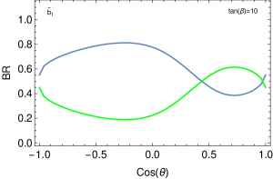
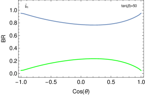
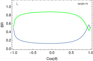
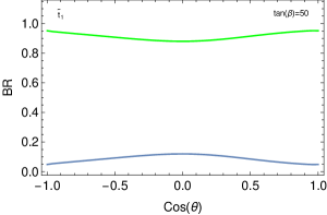
Figure 1: Branching ratios of the light stop and the light sbottom taking $m_{\tilde{q}_{1}}=500$ GeV ($q=b,t$), $m_{\tilde{\nu}_{R}}=100$ GeV, $\mu=590$ GeV, $M_{1}=M_{2}=1$ TeV. The upper row shows sbottom decays, the lower row stop decays. The left column displays the case $\tan\beta=10$ and right one $\tan\beta=50$. The lines correspond to $\tilde{q}_{1}\to q\nu\tilde{\nu}_{R}$ (blue line) and $\tilde{q}_{1}\to q^{\prime}l\tilde{\nu}_{R}$ (green line) summing over all lepton flavours. By construction each lepton flavour has the same probability.

A typical example for the branching ratios is shown in Fig. 1. An important observation is that for large $\tan\beta$ the final states containing a $t$-quark get reduced and correspondingly the final states with a $b$-quark are enhanced. The reason is that for smaller $\tan\beta$ the kinematical differences are compensated to some extent by the differences in the corresponding Yukawa couplings. The kink in the stop branching ratios close to $\cos\theta_{\tilde{t}}=0.95$ is due to a negative interference between the higgsino component, which is suppressed by $\sin\theta_{\tilde{t}}$, and the gaugino component of the $\tilde{t}_{1}$-$b$-$\tilde{\chi}^{+}_{1}$ coupling.

III Set-up and parameter space scan

For this investigation we have used a series of public programs: As a first step we have used SARAH Staub:2008uz ; Staub:2013tta ; Staub:2012pb ; Staub:2010jh ; Staub:2009bi in the SUSY/BSM toolbox 1.2.9 Staub:2011dp ; Staub:2015kfa to implement the aforementioned model into the event generator WHIZARD 2.2.6 Kilian:2007gr ; Moretti:2001zz . We use the CTEQ6L1 PDF set Pumplin:2002vw in WHIZARD, which uses PYTHIA 6.427 Sjostrand:2006za internally for showering and hadronization with the ATLAS AUET2B-CT6L tune to generate events at tree-level. The parameter scan has been automated using gnu-parallel Tange2011a . As default we generate 25000 events for every production process via strong interactions, e.g. for $pp\to\tilde{t}_{1}\tilde{t}_{1}^{*}$. The generated events are then fed in the HEPMC Dobbs:2001ck format into CheckMATE 1.2.0 Drees:2013wra that uses internally a modified version of Delphes as detector simulation deFavereau:2013fsa , FastJet Cacciari:2011ma ; Cacciari:2005hq to define jets via the anti-$k_{T}$ algorithm Cacciari:2008gp . These event samples are then re-weighted according to the corresponding total cross-section which we compute with PROSPINO 2.1 Beenakker:1996ch ; Beenakker:1997ut to get a more reliable result. CheckMATE compares the number of events passing each signal region of every considered analysis with the observed $S95$ limit obtained by the ATLAS collaboration via the parameter

$$r^{c}_{exp/obs}=\frac{S-1.96\cdot\Delta S}{S^{95}_{exp/obs}}$$ (14)

with $S$ being the number of the considered signal region, $\Delta S$ as the error from the Monte Carlo and $S^{95}_{exp/obs}$ is the expected or experimentally observed 95% confidence limit on the signal Drees:2013wra ; Drees:2015aeo .

CheckMATE contains also CMS analyses which we did not exploit here for a practical reason: in the version used one can combine easily different analyses carried out by one collaboration in a single run but not those carried out by two different collaborations. Thus their inclusion would have nearly doubled our computation time. In view of the fact, that both collaborations have obtained rather similar results, we do not expect any significant differences from the results obtained here compared to the combined analyses of both collaborations. The analyses used here are listed in table 1 together with their main characteristics.

Table 1: List of the ATLAS analyses used in this study.

Ref.	CheckMATE analysis name	Search for…	…in finals states with…
multilepton:
Aad:2014pda	atlas_1403_2500	$\tilde{g}$ and $\tilde{q}$	jets, 2SS/3 leptons
ATLAS-CONF-2013-036	atlas_conf_2013_036	$R$PV & $R$PC SUSY	four or more leptons
Aad:2014nua	atlas_1402_7029	$\tilde{\chi}^{\pm}$ and $\tilde{\chi}^{0}$	3 leptons and $\not{E}_{T}$
dilepton:
Aad:2014qaa	atlas_1403_4853	$\tilde{t}$	two leptons and 2 $b$ jets
Aad:2014vma	atlas_1403_5294	$\tilde{\ell},\tilde{\chi}^{0,\pm}$	two leptons and $\not{E}_{T}$
ATLAS-CONF-2013-089	atlas_conf_089	$\tilde{t}$	two leptons via the razor variable
ATLAS-CONF-2013-049	atlas_conf_2013_049	$\tilde{\chi}^{0,\pm},\tilde{\ell}$	two leptons
ATLAS-CONF-2014-014	atlas_conf_2013_014	$\tilde{t}$	2 $b$ jets, two leptons (vie $\tau$), $\not{E}_{T}$
single lepton:
Aad:2014kra	atlas_1407_0583	$\tilde{t}$	1 lepton, jets and $\not{E}_{T}$
ATLAS-CONF-2013-062	atlas_conf_2013_062	$\tilde{t},\tilde{g}$	1 lepton, jets and $\not{E}_{T}$
ATLAS-CONF-2012-104	atlas_conf_2013_104	$\tilde{t}$	1 lepton, jets and $\not{E}_{T}$
hadronic:
ATLAS-CONF-2013-061	atlas_conf_2013_061	$\tilde{g}$	three $b$-jets and $\not{E}_{T}$
Aad:2013ija	atlas_1308_2631	$\tilde{b},\tilde{t}$	2 $b$ jets and $\not{E}_{T}$
ATLAS-CONF-2013-047	atlas_conf_2013_047	$\tilde{q},\tilde{g}$	jets and $\not{E}_{T}$
ATLAS-CONF-2013-024	atlas_conf_2013_024	$\tilde{t}$	hadronic $t\bar{t}$ final states

The fact, that we consider a $\tilde{\nu}_{R}$ LSP implies that we expect on average more charged leptons in the final state than in the conventional Natural SUSY scenarios. This implies that the relative importance of the analyses gets changed on which we want to comment. Obviously the realm of multilepton searches is of much bigger importance in our case, in particular due to the better detectability of the leptons compared to jets. A prominent example where this is important are those containing the decay $\tilde{b}_{1}\to\tilde{\chi}^{\pm}t\to l\tilde{\nu}_{R}t$, where the chargino can be either on- or off-shell, and additional lepton(s) from the $t$ decay(s). Another example are scenarios containing decays like $\tilde{t}_{1}\to\tilde{b}W^{\pm}\to t\ell\tilde{\nu}_{R}W^{\pm}$ where the $W$ decays into leptons.

Dilepton searches retain their importance, especially in the derivation of limits for $\tilde{t}_{1}$ via the process $\tilde{t}\to\tilde{\chi}^{\pm}b\ell$ via an on- or off-shell $\tilde{\chi}^{\pm}_{1}$ in the $2\ell 2b\not{E}_{T}$ final state. This has also been observed in Guo:2013asa where exclusion limits considering only $\tilde{t}$ via the process $\tilde{t}_{1}\to\tilde{\nu}_{R}b\ell$ have been investigated in. Monolepton searches, mostly in combination with the requirement of two tagged $b$-jets are also of significance in cases where the above mentioned scenario either competes with a ’standard’ decay $\tilde{b}_{1}\to b\tilde{\chi}^{0}_{1/2}\to b\nu\tilde{\nu}_{R}$, or the process $\tilde{t}_{1}\to t\nu\tilde{\nu}_{R}$ is the dominant decay channel for the $\tilde{t}_{1}$, such one arrives at the well known $t+\not{E}_{T}$ signal.

There are also scenarios where purely hadronic searches are important. From these especially atlas_1308_2631, where a search for $\tilde{t},\tilde{b}$ via $2b+\not{E}_{T}$ is presented, is important as it covers the case of $\tilde{b}\to b\nu\tilde{\nu}_{R}$ and exploits the presence of tagable $b$-jets in the corresponding final states. Note, however, that this analysis relies on requirements of very hard jets, where the leading jet is required to have $p_{T}>150$ GeV, and large missing energy. Here one has potentially only a small acceptance in cases with moderate or small mass differences. This is especially pronounced in its signal region B, that focusses on small mass differences between third-generation squark and LSP with the trade-off to need hard ISR or FSR. As we only simulate the tree-level process without hard initial state radiation (ISR) and/or final state radiation (FSR) we often do not meet the requirements of this signal region. However, we take the resulting uncertainty into account in the interpretation of the CheckMATE result. We follow ref. Drees:2015aeo in the categorization of the CheckMATE results: we define every point as either ‘strictly allowed’ if $r^{c}_{obs}<\frac{2}{3}$, as ‘strictly excluded’ if $r^{c}_{obs}>1.5$ and ‘inconclusive’ or ‘ambiguous” in case of $\frac{2}{3}<r^{c}_{obs}<1.5$. This aids in keeping our statements less dependent on statistical fluctuations and thus more conservative. Moreover, we do not expect that the inclusion of higher order corrections will change the $r$ value such, that it switches from ‘strictly allowed’ to ‘strictly excluded’ or vice versa. Our procedure of labelling a parameter space combination as ‘strictly excluded’ differs slightly from the CheckMATE procedure: While CheckMATE takes the $r_{obs}^{c}$ value of the largest $r_{exp}^{c}$ to find its exclusion statement, we also check all other analyses with $r_{exp}^{c}>1.0$ for $r_{obs}^{c}>1.5$. If there is at least one analysis that excludes this parameter point, we take it as strictly excluded. If there is no such analysis, we take the statement given by CheckMATE.

We have chosen a regular grid in the parameter space instead of performing a random scan to get a better understanding of the different features and potential pitfalls when interpreting the results. The grid is given by combining the following parameters for the values given:

• $m_{\tilde{t}_{1}}$ in GeV: 300, 400, 500, 600, 700, 800, 900, 1000

• $m_{\tilde{b}_{1}}$ in GeV: 300, 400, 500, 600, 700, 800, 900, 1000

• $m_{\tilde{\nu}_{R}}$ in GeV : 60, 100, 200, 300, 400, 500

• $\mu$ in GeV: 110, 190, 290, 390, 490, 590 and require $m_{\tilde{\nu}_{R}}<\mu$

• $\tan\beta$: 10, 50

• $\theta_{\tilde{t}}$: $0^{\circ},45^{\circ},90^{\circ}$

• $\theta_{\tilde{b}}$: $0^{\circ},45^{\circ},90^{\circ}$

• $M_{1}=M_{2}=1$ TeV

• everything else, including $\tilde{t}_{2}$,$\tilde{b}_{2}$ and $m_{\tilde{g}}$: 2 TeV
  The exception is potentially $m_{\tilde{b}_{2}}$ when eq. (4) becomes effective as mentioned above.

IV Results

An obvious constraint for our model are searches for electroweakinos and sleptons which probe the final state resulting from the pair production of charginos and their decays:

$$pp\to\tilde{\chi}^{+}_{1}\tilde{\chi}^{-}_{1}\to\ell^{+}\ell^{-}\tilde{\nu}_{R}\tilde{\nu}^{*}_{R}\quad.$$ (15)

This decay of pair produced $\tilde{\chi}^{\pm}_{1}$ which can already restrict the $(m_{\tilde{\chi}},m_{\tilde{\nu}_{R}})$ mass plane in the dilepton channel. However the related process in eq. (11) is much more challenging, as it would manifest itself only in a monojet signature Dreiner:2012gx . It has been shown in Barducci:2015ffa that existing LHC data does not restrict the values for $\mu$ considered here from mono-jet searches and, thus, our findings are not affected by the fact that we do not take ISR into account here.

From the relevant searches, atlas_conf_2013_049 ATLAS-CONF-2013-049 and atlas_1403_5294 Aad:2014vma , the latter is more important than the first one as already noted in Arina:2015uea . The reason is that the decay kinematics of $\tilde{\ell}^{\pm}\to\ell\tilde{\chi}^{0}_{1}$ is essentially the same as in our case whereas those of $\tilde{\chi}^{+}_{1}\to\tilde{\chi}^{0}_{1}W^{+}$ show a substantial difference. The impact of these analyses on the parameter space is shown in Fig. (2).

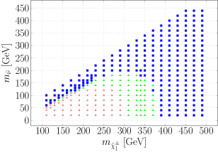
Figure 2: Exclusions in the $(m_{\tilde{\chi}^{\pm}},m_{\tilde{\nu}_{R}})$ mass plane derived from the ATLAS searches ATLAS-CONF-2013-049 and Aad:2014vma : points with a $\color[rgb]{1,0,0}\times$ are excluded, $\color[rgb]{0,1,0}\blacktriangle$ designate points as ambigous, whereas points with $\color[rgb]{0,0,1}\blacksquare$ are still allowed.

This allows to exclude parameter combinations containing the $(m_{\tilde{\chi}^{\pm}},m_{\tilde{\nu}_{R}})$ combinations $(190,60),(190,100)$ and $(290,60)$ from further consideration.

For the investigation of the remaining parameter space we calculate as default the rates for the processes

$$pp\to\quad\tilde{b}_{1}\tilde{b}_{1}^{*},\quad\tilde{t}_{1}\tilde{t}_{1}^{*}\quad.$$ (16)

For scenarios where the application of eq. (4) results in $m_{\tilde{b}_{2}}<1000$ GeV, we calculate also the rate for

$$pp\to\tilde{b}_{2}\tilde{b}_{2}^{*}\quad.$$

In such scenarios it can happen that the calculated mass for $\tilde{b}_{2}$ is actually smaller than the input value for $\tilde{b}_{1}$. If this happens we flip the resulting mass hierarchy as we want to keep the default $m_{\tilde{b}_{1}}<m_{\tilde{b}_{2}}$. We denote those as ‘flipped’ point/case and treat them separately at the end of this section.

We start by presenting our findings for various parameter combinations in the $m_{\tilde{t}_{1}}$-$m_{\tilde{b}_{1}}$ and refer for more details to the coming ref. DissLukas . A short summary explaining the entries of the plots in Figs. 4–8 is given in Fig. 3. At every point in the $m_{\tilde{t}_{1}}$-$m_{\tilde{b}_{1}}$ we display all considered combinations of mixing angles in the stop and sbottom sector by slightly shifting the result depending on the respective mixing angle: The right column represents scenarios with a right stop and a right sbottom, i.e. $\tilde{t}_{1}=\tilde{t}_{R}$. The middle column belongs to a maximally mixed stop whereas the left column consists of all points with a left stop $\tilde{t}_{1}=\tilde{t}_{L}$, i.e. $\theta_{\tilde{t}}=0$. In the scenarios of this column we use the tree-level relation (4) as discussed above. Note, that even if no flipping of the sbottom masses takes place, one might have additional signals coming from the production of the heavier sbottom. The different rows belong to different mixing angles in the sbottom sector: The top one corresponds to $\theta_{\tilde{b}}=0$, the middle one to $\theta_{\tilde{b}}=45^{\circ}$ and the lowest one to $\theta_{\tilde{b}}=90^{\circ}$.

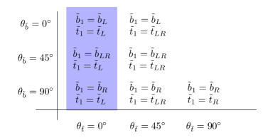
Figure 3: Infographic explaining the $3\times 3$ blocks at the various parameter points in Figs. 4–8: they correspond to the different combinations of sbottom and stop mixing angles shown here. The case $\tilde{\theta}_{t}$ is special as there eq. (4) needs to be considered.

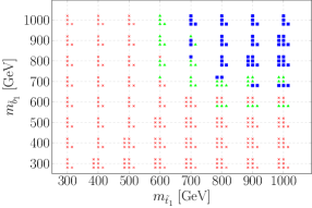
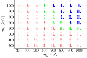
Figure 4: Parameter space points excluded or allowed by the searches listed in Tab. 1 for $\mu=110$ GeV, $m_{\tilde{\nu}_{R}}=60$ GeV, $\tan\beta=10$ (left) and for $\tan\beta=50$ (right). At each ($m_{\tilde{t}},m_{\tilde{b}_{1}}$) mass pair one finds a $3\times 3$ block representing the different combinations of the mixing angles in the $\tilde{t}$ and the $\tilde{b}$ sector (see Fig. 3). $\color[rgb]{1,0,0}\times$ designate points excluded by CheckMATE, $\color[rgb]{0,1,0}\blacktriangle$ designate points as ambigous, while $\color[rgb]{0,0,1}\blacksquare$ indicate points still allowed by the considered ATLAS analyses.

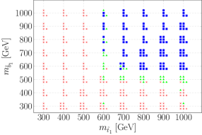
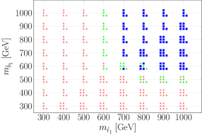
Figure 5: The same as Fig. 4 but for $m_{\tilde{\nu}_{R}}=100$ GeV.

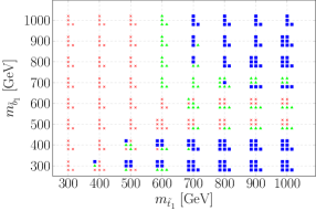
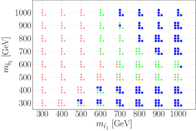
Figure 6: The same as Fig. 4 but for $\mu=290$ GeV and $m_{\tilde{\nu}_{R}}=200$ GeV.

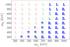
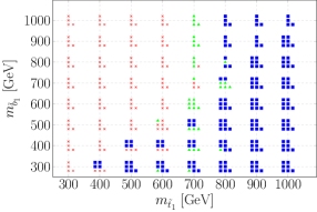
Figure 7: The same as Fig. 4 but for $\mu=490$ GeV and $m_{\tilde{\nu}_{R}}=200$ GeV.

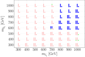
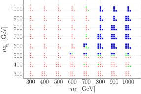
Figure 8: The same as Fig. 4 but for $\mu=590$ GeV.

In Figures 4–8 we display those points where the mass ordering of the sbottoms is not changed. We comment on the flipped sbottom mass scenarios at the end of this section as they hardly lead to new features. Figure 4 shows the case with a rather hierarchical mass spectrum. As a result the final states contain several hard leptons implying the stop and sbottom masses below about 500 GeV can be excluded. For larger values the cross sections get so much reduced that one would have to take higher order corrections into account. Moreover, these cases would have required more detailed experimental investigations as the experimental cuts are most likely not optimized for these cases. In case that both, ${\tilde{b}_{1}}$ and ${\tilde{t}_{1}}$, have masses above about 800 GeV, the production cross section gets too small and, thus, these scenarios are strictly allowed. Comparing the two values of $\tan\beta$ we find only a small effect: the bounds are somewhat softer for large $\tan\beta$ due to the smaller number of produced top-quarks. Note, the composition of the lepton flavours does not depend on $\tan\beta$ here as we have a pure right-handed sneutrino. In case that also the left-handed sneutrino mass parameter gets smaller, we would expect a further reduction of the bounds as the number of $\tau$-leptons would increase with a simultaneous reduction of electrons and muons in the final state.

In Figure 5 we show a scenario with a small mass difference $m_{\tilde{\chi}^{\pm}}-m_{\tilde{\nu}_{R}}=10$ GeV leading to softer leptons. As a consequence the bounds on the stop and sbottom masses get weakened by at least 100 GeV. A further reduction happens if also the mass difference between the squarks and the sneutrino gets small because then also the resulting $b$-quarks are too soft to be detected. An example is show in Fig. 6 where we have set $\mu=290$ GeV and $m_{\tilde{\nu}_{R}}=200$ GeV. In particular the sbottom searches in the $b\not{E}_{T}$ become less important because of the requirement that the jet has to have a $p_{T}$ of at least 150 GeV in the analysis atlas_1308_2631 Aad:2013ija which is not met in case of light sbottoms with a mass of 300-400 GeV. The situation is different for stops with such a mass as there the decay into $b\tilde{\chi}^{+}_{1}\to bl\tilde{\nu}_{R}$ is present and thus the lepton searches are effective.

An increase in $\mu$ leads to a merger of the allowed region created by the compressed mass spectrum with the high-masses allowed region, as can be seen in the trend going from Fig. 6 to Fig. 7. However the size of this allowed region is still dependent on the mass of $\tilde{\nu}_{R}$ as can be observed in a comparison of Fig. 7 and Fig. 8. In particular in the later case only three-body decays of the squarks are possible if their masses are below 600 GeV resulting in hard $b$-jets and leptons and thus to a larger excluded region in the $m_{\tilde{t}_{1}}$–$m_{\tilde{b}_{1}}$ plane compared to the previous case.

a)			b)
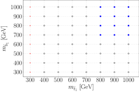
c)			d)

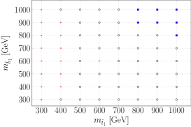
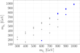
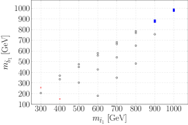
Figure 9: Summary plots in the $m_{\tilde{t}_{1}}$–$m_{\tilde{b}_{1}}$ plane marginalized over all allowed and considered $\tilde{\theta}_{b}$, $\tilde{\theta}_{t}$, $\tan\beta$, $\mu$ and $m_{\tilde{\nu}_{R}}$ combinations. A point denoted by $\color[rgb]{1,0,0}\times$ is excluded for all combinations, for a point with $\circ$ the exclusion depends on the parameter space combination, while points with a $\color[rgb]{0,0,1}\blacksquare$ are allowed for all parameter combinations. The different plots correspond to: a) Counting ’ambiguous’ points conservatively as allowed in cases where no flipping in the sbottom mass hierarchy occurred. b) Counting ’ambiguous’ points as excluded in cases where no flipping in the sbottom mass hierarchy occurred. c) Counting ’ambiguous’ points conservatively as allowed in cases where a flipping in the sbottom mass hierarchy occurred. d) Counting ’ambiguous’ points as excluded in cases where a flipping in the sbottom mass hierarchy occurred.

In Figure 9 we summarize the exclusion statements in a condensed way. We put the ’ambiguous’ either conservatively to the set of allowed points (left column) or to the excluded set (right column) to get a rough idea of the underlying uncertainty. The upper row gives the cases with an unflipped sbottom mass spectrum. We see in plot a) that only the case of $m_{\tilde{t}_{1}}=300$ GeV is strictly excluded if the ambiguous points are counted as allowed. The corner with $m_{\tilde{b}_{1}}\geq 700$GeV and $m_{\tilde{t}_{1}}\geq 800$ GeV is not constrained at all which was expected due to the small production cross section. The exclusion statement for all other points is strongly dependent on the underlying parameter combinations as can be seen from the discussion of the individual cases before. A comparison with the right column shows that the range of excluded stop masses for all other parameter combinations gets somewhat larger if the ambiguous points are counted as excluded indicating that this region deserves further investigations. This also correct for some parameter combinations in the the higher stop and sbottom mass region close to 800 GeV. A particular case is $m_{\tilde{t}_{1}}=m_{\tilde{b}_{1}}=600$ GeV which seems now to be excluded for all parameter combinations. However, this has to be taken with a grain of salt as we have restricted $\mu\leq 590$ GeV and, thus, having always two-body decays. We have also checked that this point is not excluded, which means having $r^{c}_{obs}$ values below 2/3, for some parameter combinations if only three body decays of the squarks are allowed by setting $\mu=610$ GeV for this particular case.

The lower row gives the cases where the sbottom mass ordering is flipped. Here we exclude right from the start all points where the sbottom is lighter than the sneutrino. We see that these cases are consistent with the findings in the upper row. However, in addition we have here a couple of points where the lighter sbottom has a mass below 300 GeV. It is intriguing that in the rather low mass region the exclusion depends on the parameter combinations in the conservative case (left side). The reason for this lies in the particular mass hierarchies: in cases, where the decay $\tilde{t}_{1}\to W^{+}\tilde{b}_{1}$ is the only viable one due to a large $\mu$, the value of the sneutrino mass determines the $p_{T}$ and visibility of the exiting $b$ quark which helps to pass the particular analysis’ jet requirements in addition to the jets coming from the $W$. Moreover, the mass splitting between $\tilde{t}_{1}$ and $\tilde{b}_{1}$ is rather small leaving little phase space for the $W$-boson which in turn implies that the resulting jet energies hardly pass the required $p_{T}$-cuts.

A comparison of our exclusion with those ref. Guo:2013asa shows that due the fact, that we do not only consider $\cos\theta_{\tilde{t}}=0$, implying $\tilde{t}_{1}=\tilde{t}_{R}$, but consider three different values, we do not reach their strict exclusions of $m_{\tilde{t}_{1}}$ up to 900 GeV. However, if for a pure $\tilde{t}_{R}$ we do not reach this value which is due to the differences between CheckMATE and PGS. Similarly, we get lower bounds on the mass bounds of the chargino and sneutrinos from the direct chargino production: we get roughly a bound of $m_{\tilde{\chi}^{\pm}}\sim 300$ GeV and $m_{\tilde{\nu}_{R}}\sim 120$ GeV whereas in Guo:2013asa the bounds $m_{\tilde{\chi}^{\pm}}\sim 550$ GeV and $m_{\tilde{\nu}_{R}}\sim 300$ GeV. The main difference is the more conservative $r^{c}_{obs}$-measure of CheckMATE given in eq. (14) whereas in PGS the measure $R=\frac{N_{NP}}{N_{limit}}$ is used with $N_{NP}$ and $N_{limit}$ being the number of events from the new physics and the experimental upper bound, respectively.

V Conclusions

In this paper we have studied a variant of the natural supersymmetric models containing a right-handed sneutrino LSP as it can emerge as effective model from models with extended gauge groups. We have considered different scenarios taking also into account the case that at least one of the sbottoms gets light. The latter can in particular occur if the lighter stop is essentially left-handed. Provided that the mass difference is not too small we find that only stop masses of up to about 300 GeV can be excluded in this scenario independent of its nature. Depending on the scenario, where the main parameters are the stop mixing angles and the ratio of stop mass to $\mu$ to sneutrino mass, one can exclude larger masses of up to 700 GeV. Here we roughly confirm the findings of Guo:2013asa where the case of a pure $\tilde{t}_{R}$ had been considered. In addition we obtain similar results for the sbottoms. Last but not least we find that the bounds are somewhat weaker in case of large $\tan\beta$ as the number of produced $t$-quarks from the squark decays is smaller which in turn reduces the average number of hard leptons in the final state.

References

- (1) ATLAS Collaboration, G. Aad et al., “Observation of a new particle in the search for the Standard Model Higgs boson with the ATLAS detector at the LHC,” Phys. Lett. B716 (2012) 1–29, arXiv:1207.7214 [hep-ex].
- (2) CMS Collaboration, S. Chatrchyan et al., “Observation of a new boson at a mass of 125 GeV with the CMS experiment at the LHC,” Phys. Lett. B716 (2012) 30–61, arXiv:1207.7235 [hep-ex].
- (3) ATLAS, CMS Collaboration, G. Aad et al., “Combined Measurement of the Higgs Boson Mass in Collisions at and 8 TeV with the ATLAS and CMS Experiments,” Phys. Rev. Lett. 114 (2015) 191803, arXiv:1503.07589 [hep-ex].
- (4) C. Brust, A. Katz, S. Lawrence, and R. Sundrum, “SUSY, the Third Generation and the LHC,” JHEP 03 (2012) 103, arXiv:1110.6670 [hep-ph].
- (5) M. Papucci, J. T. Ruderman, and A. Weiler, “Natural SUSY Endures,” JHEP 09 (2012) 035, arXiv:1110.6926 [hep-ph].
- (6) L. J. Hall, D. Pinner, and J. T. Ruderman, “A Natural SUSY Higgs Near 126 GeV,” JHEP 04 (2012) 131, arXiv:1112.2703 [hep-ph].
- (7) K. Blum, R. T. D’Agnolo, and J. Fan, “Natural SUSY Predicts: Higgs Couplings,” JHEP 01 (2013) 057, arXiv:1206.5303 [hep-ph].
- (8) J. R. Espinosa, C. Grojean, V. Sanz, and M. Trott, “NSUSY fits,” JHEP 12 (2012) 077, arXiv:1207.7355 [hep-ph].
- (9) R. T. D’Agnolo, E. Kuflik, and M. Zanetti, “Fitting the Higgs to Natural SUSY,” JHEP 03 (2013) 043, arXiv:1212.1165.
- (10) H. Baer, V. Barger, P. Huang, and X. Tata, “Natural Supersymmetry: LHC, dark matter and ILC searches,” JHEP 05 (2012) 109, arXiv:1203.5539 [hep-ph].
- (11) J. E. Younkin and S. P. Martin, “Non-universal gaugino masses, the supersymmetric little hierarchy problem, and dark matter,” Phys. Rev. D85 (2012) 055028, arXiv:1201.2989 [hep-ph].
- (12) G. D. Kribs, A. Martin, and A. Menon, “Natural Supersymmetry and Implications for Higgs physics,” Phys. Rev. D88 (2013) 035025, arXiv:1305.1313 [hep-ph].
- (13) E. Hardy, “Is Natural SUSY Natural?,” JHEP 10 (2013) 133, arXiv:1306.1534 [hep-ph].
- (14) K. Kowalska and E. M. Sessolo, “Natural MSSM after the LHC 8 TeV run,” Phys. Rev. D88 no. 7, (2013) 075001, arXiv:1307.5790 [hep-ph].
- (15) C. Han, K.-i. Hikasa, L. Wu, J. M. Yang, and Y. Zhang, “Current experimental bounds on stop mass in natural SUSY,” JHEP 10 (2013) 216, arXiv:1308.5307 [hep-ph].
- (16) H. P. Nilles, M. Srednicki, and D. Wyler, “Weak Interaction Breakdown Induced by Supergravity,” Phys. Lett. B120 (1983) 346.
- (17) J. P. Derendinger and C. A. Savoy, “Quantum Effects and SU(2) x U(1) Breaking in Supergravity Gauge Theories,” Nucl. Phys. B237 (1984) 307.
- (18) J. R. Ellis, J. F. Gunion, H. E. Haber, L. Roszkowski, and F. Zwirner, “Higgs Bosons in a Nonminimal Supersymmetric Model,” Phys. Rev. D39 (1989) 844.
- (19) M. Drees, “Supersymmetric Models with Extended Higgs Sector,” Int. J. Mod. Phys. A4 (1989) 3635.
- (20) U. Ellwanger, M. Rausch de Traubenberg, and C. A. Savoy, “Particle spectrum in supersymmetric models with a gauge singlet,” Phys. Lett. B315 (1993) 331–337, arXiv:hep-ph/9307322 [hep-ph].
- (21) S. F. King and P. L. White, “Resolving the constrained minimal and next-to-minimal supersymmetric standard models,” Phys. Rev. D52 (1995) 4183–4216, arXiv:hep-ph/9505326 [hep-ph].
- (22) F. Franke and H. Fraas, “Neutralinos and Higgs bosons in the next-to-minimal supersymmetric standard model,” Int. J. Mod. Phys. A12 (1997) 479–534, arXiv:hep-ph/9512366 [hep-ph].
- (23) U. Ellwanger and C. Hugonie, “The Upper bound on the lightest Higgs mass in the NMSSM revisited,” Mod. Phys. Lett. A22 (2007) 1581–1590, arXiv:hep-ph/0612133 [hep-ph].
- (24) H. E. Haber and M. Sher, “Higgs Mass Bound in Based Supersymmetric Theories,” Phys. Rev. D35 (1987) 2206.
- (25) M. Drees, “Comment on ‘Higgs Boson Mass Bound in Based Supersymmetric Theories.’,” Phys. Rev. D35 (1987) 2910–2913.
- (26) M. Cvetic, D. A. Demir, J. R. Espinosa, L. L. Everett, and P. Langacker, “Electroweak breaking and the mu problem in supergravity models with an additional U(1),” Phys. Rev. D56 (1997) 2861, arXiv:hep-ph/9703317 [hep-ph]. [Erratum: Phys. Rev.D58,119905(1998)].
- (27) Y. Zhang, H. An, X.-d. Ji, and R. N. Mohapatra, “Light Higgs Mass Bound in SUSY Left-Right Models,” Phys. Rev. D78 (2008) 011302, arXiv:0804.0268 [hep-ph].
- (28) E. Ma, “Exceeding the MSSM Higgs Mass Bound in a Special Class of U(1) Gauge Models,” Phys. Lett. B705 (2011) 320–323, arXiv:1108.4029 [hep-ph].
- (29) M. Hirsch, M. Malinsky, W. Porod, L. Reichert, and F. Staub, “Hefty MSSM-like light Higgs in extended gauge models,” JHEP 02 (2012) 084, arXiv:1110.3037 [hep-ph].
- (30) ATLAS Collaboration, G. Aad et al., “Search for direct third-generation squark pair production in final states with missing transverse momentum and two -jets in 8 TeV collisions with the ATLAS detector,” JHEP 10 (2013) 189, arXiv:1308.2631 [hep-ex].
- (31) ATLAS Collaboration, G. Aad et al., “Search for direct production of charginos, neutralinos and sleptons in final states with two leptons and missing transverse momentum in collisions at 8 TeV with the ATLAS detector,” JHEP 05 (2014) 071, arXiv:1403.5294 [hep-ex].
- (32) ATLAS Collaboration, G. Aad et al., “Search for pair-produced third-generation squarks decaying via charm quarks or in compressed supersymmetric scenarios in collisions at TeV with the ATLAS detector,” Phys. Rev. D90 no. 5, (2014) 052008, arXiv:1407.0608 [hep-ex].
- (33) ATLAS Collaboration, G. Aad et al., “ATLAS Run 1 searches for direct pair production of third-generation squarks at the Large Hadron Collider,” Eur. Phys. J. C75 no. 10, (2015) 510, arXiv:1506.08616 [hep-ex].
- (34) CMS Collaboration, S. Chatrchyan et al., “Search for top-squark pair production in the single-lepton final state in pp collisions at = 8 TeV,” Eur. Phys. J. C73 no. 12, (2013) 2677, arXiv:1308.1586 [hep-ex].
- (35) CMS Collaboration, V. Khachatryan et al., “Searches for third-generation squark production in fully hadronic final states in proton-proton collisions at TeV,” JHEP 06 (2015) 116, arXiv:1503.08037 [hep-ex].
- (36) CMS Collaboration, V. Khachatryan et al., “Search for direct pair production of scalar top quarks in the single- and dilepton channels in proton-proton collisions at = 8 TeV,” arXiv:1602.03169 [hep-ex].
- (37) CMS Collaboration, V. Khachatryan et al., “Search for direct pair production of supersymmetric top quarks decaying to all-hadronic final states in pp collisions at sqrt(s) = 8 TeV,” arXiv:1603.00765 [hep-ex].
- (38) G. Brooijmans et al., “Les Houches 2013: Physics at TeV Colliders: New Physics Working Group Report,” arXiv:1405.1617 [hep-ph].
- (39) M. Drees and J. S. Kim, “Natural Supersymmetry after the LHC8,” arXiv:1511.04461 [hep-ph].
- (40) A. Kobakhidze, N. Liu, L. Wu, J. M. Yang, and M. Zhang, “Closing up a light stop window in natural SUSY at LHC,” Phys. Lett. B755 (2016) 76–81, arXiv:1511.02371 [hep-ph].
- (41) J. Fan, R. Krall, D. Pinner, M. Reece, and J. T. Ruderman, “Stealth Supersymmetry Simplified,” arXiv:1512.05781 [hep-ph].
- (42) G. Chalons and D. Sengupta, “Closing in on compressed gluino-neutralino spectra at the LHC,” arXiv:1508.06735 [hep-ph].
- (43) J. S. Kim, D. Schmeier, and J. Tattersall, “Naughty or Nice? The Role of the ‘N’ in the Natural NMSSM for the LHC,” arXiv:1510.04871 [hep-ph].
- (44) J. Guo, Z. Kang, J. Li, T. Li, and Y. Liu, “Simplified Supersymmetry with Sneutrino LSP at 8 TeV LHC,” JHEP 10 (2014) 164, arXiv:1312.2821 [hep-ph].
- (45) P. Minkowski, “ at a Rate of One Out of Muon Decays?,” Phys. Lett. B67 (1977) 421–428.
- (46) T. Yanagida, “HORIZONTAL SYMMETRY AND MASSES OF NEUTRINOS,” Conf.Proc. C7902131 (1979) 95.
- (47) R. N. Mohapatra and G. Senjanovic, “Neutrino Mass and Spontaneous Parity Violation,” Phys. Rev. Lett. 44 (1980) 912.
- (48) M. Gell-Mann, P. Ramond, and R. Slansky, “Complex Spinors and Unified Theories,” Conf. Proc. C790927 (1979) 315–321, arXiv:1306.4669 [hep-th].
- (49) J. Schechter and J. W. F. Valle, “Neutrino Masses in SU(2) x U(1) Theories,” Phys. Rev. D22 (1980) 2227.
- (50) A. de Gouvea, S. Gopalakrishna, and W. Porod, “Stop Decay into Right-handed Sneutrino LSP at Hadron Colliders,” JHEP 11 (2006) 050, arXiv:hep-ph/0606296 [hep-ph].
- (51) CMS Collaboration, S. Chatrchyan et al., “Searches for long-lived charged particles in pp collisions at =7 and 8 TeV,” JHEP 07 (2013) 122, arXiv:1305.0491 [hep-ex].
- (52) ATLAS Collaboration, G. Aad et al., “Searches for heavy long-lived charged particles with the ATLAS detector in proton-proton collisions at TeV,” JHEP 01 (2015) 068, arXiv:1411.6795 [hep-ex].
- (53) R. N. Mohapatra and J. W. F. Valle, “Neutrino Mass and Baryon Number Nonconservation in Superstring Models,” Phys. Rev. D34 (1986) 1642.
- (54) C. Arina, M. E. C. Catalan, S. Kraml, S. Kulkarni, and U. Laa, “Constraints on sneutrino dark matter from LHC Run 1,” JHEP 05 (2015) 142, arXiv:1503.02960 [hep-ph].
- (55) G. Bélanger, J. Da Silva, U. Laa, and A. Pukhov, “Probing U(1) extensions of the MSSM at the LHC Run I and in dark matter searches,” JHEP 09 (2015) 151, arXiv:1505.06243 [hep-ph].
- (56) S. Kraml, S. Kulkarni, U. Laa, A. Lessa, W. Magerl, D. Proschofsky-Spindler, and W. Waltenberger, “SModelS: a tool for interpreting simplified-model results from the LHC and its application to supersymmetry,” Eur. Phys. J. C74 (2014) 2868, arXiv:1312.4175 [hep-ph].
- (57) M. Drees, H. Dreiner, D. Schmeier, J. Tattersall, and J. S. Kim, “CheckMATE: Confronting your Favourite New Physics Model with LHC Data,” Comput. Phys. Commun. 187 (2014) 227–265, arXiv:1312.2591 [hep-ph].
- (58) R. Mahbubani, M. Papucci, G. Perez, J. T. Ruderman, and A. Weiler, “Light Nondegenerate Squarks at the LHC,” Phys. Rev. Lett. 110 no. 15, (2013) 151804, arXiv:1212.3328 [hep-ph].
- (59) M. Papucci, K. Sakurai, A. Weiler, and L. Zeune, “Fastlim: a fast LHC limit calculator,” Eur. Phys. J. C74 no. 11, (2014) 3163, arXiv:1402.0492 [hep-ph].
- (60) J. Conway, “www.physics.ucdavis.edu/conway/research/software/pgs/pgs4-general.htm.”.
- (61) E. Conte, B. Fuks, and G. Serret, “MadAnalysis 5, A User-Friendly Framework for Collider Phenomenology,” Comput. Phys. Commun. 184 (2013) 222–256, arXiv:1206.1599 [hep-ph].
- (62) E. Conte, B. Dumont, B. Fuks, and C. Wymant, “Designing and recasting LHC analyses with MadAnalysis 5,” Eur. Phys. J. C74 no. 10, (2014) 3103, arXiv:1405.3982 [hep-ph].
- (63) B. Dumont, B. Fuks, S. Kraml, S. Bein, G. Chalons, E. Conte, S. Kulkarni, D. Sengupta, and C. Wymant, “Toward a public analysis database for LHC new physics searches using MADANALYSIS 5,” Eur. Phys. J. C75 no. 2, (2015) 56, arXiv:1407.3278 [hep-ph].
- (64) S. Gopalakrishna, A. de Gouvea, and W. Porod, “Right-handed sneutrinos as nonthermal dark matter,” JCAP 0605 (2006) 005, arXiv:hep-ph/0602027 [hep-ph].
- (65) T. Asaka, K. Ishiwata, and T. Moroi, “Right-handed sneutrino as cold dark matter of the universe,” Phys. Rev. D75 (2007) 065001, arXiv:hep-ph/0612211 [hep-ph].
- (66) H.-S. Lee, K. T. Matchev, and S. Nasri, “Revival of the thermal sneutrino dark matter,” Phys. Rev. D76 (2007) 041302, arXiv:hep-ph/0702223 [HEP-PH].
- (67) C. Arina and N. Fornengo, “Sneutrino cold dark matter, a new analysis: Relic abundance and detection rates,” JHEP 11 (2007) 029, arXiv:0709.4477 [hep-ph].
- (68) Z. Thomas, D. Tucker-Smith, and N. Weiner, “Mixed Sneutrinos, Dark Matter and the CERN LHC,” Phys. Rev. D77 (2008) 115015, arXiv:0712.4146 [hep-ph].
- (69) F. Deppisch and A. Pilaftsis, “Thermal Right-Handed Sneutrino Dark Matter in the F(D)-Term Model of Hybrid Inflation,” JHEP 10 (2008) 080, arXiv:0808.0490 [hep-ph].
- (70) D. G. Cerdeno and O. Seto, “Right-handed sneutrino dark matter in the NMSSM,” JCAP 0908 (2009) 032, arXiv:0903.4677 [hep-ph].
- (71) A. Kumar, D. Tucker-Smith, and N. Weiner, “Neutrino Mass, Sneutrino Dark Matter and Signals of Lepton Flavor Violation in the MRSSM,” JHEP 09 (2010) 111, arXiv:0910.2475 [hep-ph].
- (72) G. Belanger, J. Da Silva, and A. Pukhov, “The Right-handed sneutrino as thermal dark matter in U(1) extensions of the MSSM,” JCAP 1112 (2011) 014, arXiv:1110.2414 [hep-ph].
- (73) V. De Romeri and M. Hirsch, “Sneutrino Dark Matter in Low-scale Seesaw Scenarios,” JHEP 12 (2012) 106, arXiv:1209.3891 [hep-ph].
- (74) M. Hirsch, W. Porod, L. Reichert, and F. Staub, “Phenomenology of the minimal supersymmetric extension of the standard model,” Phys. Rev. D86 (2012) 093018, arXiv:1206.3516 [hep-ph].
- (75) D. Barducci, A. Belyaev, A. K. M. Bharucha, W. Porod, and V. Sanz, “Uncovering Natural Supersymmetry via the interplay between the LHC and Direct Dark Matter Detection,” JHEP 07 (2015) 066, arXiv:1504.02472 [hep-ph].
- (76) A. Bartl, W. Majerotto, and W. Porod, “Squark and gluino decays for large tan beta,” Z. Phys. C64 (1994) 499–508. [Erratum: Z. Phys.C68,518(1995)].
- (77) F. Staub, “SARAH,” arXiv:0806.0538 [hep-ph].
- (78) F. Staub, “SARAH 4 : A tool for (not only SUSY) model builders,” Comput. Phys. Commun. 185 (2014) 1773–1790, arXiv:1309.7223 [hep-ph].
- (79) F. Staub, “SARAH 3.2: Dirac Gauginos, UFO output, and more,” Comput. Phys. Commun. 184 (2013) 1792–1809, arXiv:1207.0906 [hep-ph].
- (80) F. Staub, “Automatic Calculation of supersymmetric Renormalization Group Equations and Self Energies,” Comput. Phys. Commun. 182 (2011) 808–833, arXiv:1002.0840 [hep-ph].
- (81) F. Staub, “From Superpotential to Model Files for FeynArts and CalcHep/CompHep,” Comput. Phys. Commun. 181 (2010) 1077–1086, arXiv:0909.2863 [hep-ph].
- (82) F. Staub, T. Ohl, W. Porod, and C. Speckner, “A Tool Box for Implementing Supersymmetric Models,” Comput. Phys. Commun. 183 (2012) 2165–2206, arXiv:1109.5147 [hep-ph].
- (83) F. Staub, “Exploring new models in all detail with SARAH,” Adv. High Energy Phys. 2015 (2015) 840780, arXiv:1503.04200 [hep-ph].
- (84) W. Kilian, T. Ohl, and J. Reuter, “WHIZARD: Simulating Multi-Particle Processes at LHC and ILC,” Eur. Phys. J. C71 (2011) 1742, arXiv:0708.4233 [hep-ph].
- (85) M. Moretti, T. Ohl, and J. Reuter, “O’Mega: An Optimizing matrix element generator,” arXiv:hep-ph/0102195 [hep-ph].
- (86) J. Pumplin, D. R. Stump, J. Huston, H. L. Lai, P. M. Nadolsky, and W. K. Tung, “New generation of parton distributions with uncertainties from global QCD analysis,” JHEP 07 (2002) 012, arXiv:hep-ph/0201195 [hep-ph].
- (87) T. Sjostrand, S. Mrenna, and P. Z. Skands, “PYTHIA 6.4 Physics and Manual,” JHEP 05 (2006) 026, arXiv:hep-ph/0603175 [hep-ph].
- (88) O. Tange, “Gnu parallel - the command-line power tool,” ;login: The USENIX Magazine 36 no. 1, (Feb, 2011) 42–47. http://www.gnu.org/s/parallel.
- (89) M. Dobbs and J. B. Hansen, “The HepMC C++ Monte Carlo event record for High Energy Physics,” Comput. Phys. Commun. 134 (2001) 41–46.
- (90) DELPHES 3 Collaboration, J. de Favereau, C. Delaere, P. Demin, A. Giammanco, V. Lemaître, A. Mertens, and M. Selvaggi, “DELPHES 3, A modular framework for fast simulation of a generic collider experiment,” JHEP 02 (2014) 057, arXiv:1307.6346 [hep-ex].
- (91) M. Cacciari, G. P. Salam, and G. Soyez, “FastJet User Manual,” Eur. Phys. J. C72 (2012) 1896, arXiv:1111.6097 [hep-ph].
- (92) M. Cacciari and G. P. Salam, “Dispelling the myth for the jet-finder,” Phys. Lett. B641 (2006) 57–61, arXiv:hep-ph/0512210 [hep-ph].
- (93) M. Cacciari, G. P. Salam, and G. Soyez, “The Anti-k(t) jet clustering algorithm,” JHEP 04 (2008) 063, arXiv:0802.1189 [hep-ph].
- (94) W. Beenakker, R. Hopker, M. Spira, and P. M. Zerwas, “Squark and gluino production at hadron colliders,” Nucl. Phys. B492 (1997) 51–103, arXiv:hep-ph/9610490 [hep-ph].
- (95) W. Beenakker, M. Kramer, T. Plehn, M. Spira, and P. M. Zerwas, “Stop production at hadron colliders,” Nucl. Phys. B515 (1998) 3–14, arXiv:hep-ph/9710451 [hep-ph].
- (96) ATLAS Collaboration, G. Aad et al., “Search for supersymmetry at =8 TeV in final states with jets and two same-sign leptons or three leptons with the ATLAS detector,” JHEP 06 (2014) 035, arXiv:1404.2500 [hep-ex].
- (97) ATLAS Collaboration, “Search for supersymmetry in events with four or more leptons in 21 fb-1 of pp collisions at TeV with the ATLAS detector,” Tech. Rep. ATLAS-CONF-2013-036, CERN, Geneva, Mar, 2013. https://cds.cern.ch/record/1532429.
- (98) ATLAS Collaboration, G. Aad et al., “Search for direct production of charginos and neutralinos in events with three leptons and missing transverse momentum in 8TeV collisions with the ATLAS detector,” JHEP 04 (2014) 169, arXiv:1402.7029 [hep-ex].
- (99) ATLAS Collaboration, G. Aad et al., “Search for direct top-squark pair production in final states with two leptons in pp collisions at 8TeV with the ATLAS detector,” JHEP 06 (2014) 124, arXiv:1403.4853 [hep-ex].
- (100) “Search for strongly produced supersymmetric particles in decays with two leptons at = 8 TeV,” Tech. Rep. ATLAS-CONF-2013-089, CERN, Geneva, Aug, 2013. https://cds.cern.ch/record/1595272.
- (101) “Search for direct-slepton and direct-chargino production in final states with two opposite-sign leptons, missing transverse momentum and no jets in 20/fb of pp collisions at sqrt(s) = 8 TeV with the ATLAS detector,” Tech. Rep. ATLAS-CONF-2013-049, CERN, Geneva, May, 2013. http://cds.cern.ch/record/1547565.
- (102) “Search for the direct pair production of top squarks decaying to a b quark, a tau lepton, and weakly interacting particles, in pp collisions using of ATLAS data,” Tech. Rep. ATLAS-CONF-2014-014, CERN, Geneva, Mar, 2014. https://cds.cern.ch/record/1690283.
- (103) ATLAS Collaboration, G. Aad et al., “Search for top squark pair production in final states with one isolated lepton, jets, and missing transverse momentum in 8 TeV collisions with the ATLAS detector,” JHEP 11 (2014) 118, arXiv:1407.0583 [hep-ex].
- (104) “Search for squarks and gluinos in events with isolated leptons, jets and missing transverse momentum at TeV with the ATLAS detector,” Tech. Rep. ATLAS-CONF-2013-062, CERN, Geneva, Jun, 2013. https://cds.cern.ch/record/1557779.
- (105) ATLAS Collaboration Collaboration, “Search for supersymmetry at TeV in final states with jets, missing transverse momentum and one isolated lepton,” Tech. Rep. ATLAS-CONF-2012-104, CERN, Geneva, Aug, 2012. http://cds.cern.ch/record/1472673.
- (106) “Search for strong production of supersymmetric particles in final states with missing transverse momentum and at least three b-jets using 20.1 fb-1 of pp collisions at sqrt(s) = 8 TeV with the ATLAS Detector.,” Tech. Rep. ATLAS-CONF-2013-061, CERN, Geneva, Jun, 2013. http://cds.cern.ch/record/1557778.
- (107) “Search for squarks and gluinos with the ATLAS detector in final states with jets and missing transverse momentum and 20.3 fb-1 of TeV proton-proton collision data,” Tech. Rep. ATLAS-CONF-2013-047, CERN, Geneva, May, 2013. https://cds.cern.ch/record/1547563.
- (108) ATLAS Collaboration Collaboration, “Search for direct production of the top squark in the all-hadronic ttbar + etmiss final state in 21 fb-1 of p-pcollisions at sqrt(s)=8 TeV with the ATLAS detector,” Tech. Rep. ATLAS-CONF-2013-024, CERN, Geneva, Mar, 2013. https://cds.cern.ch/record/1525880.
- (109) H. K. Dreiner, M. Kramer, and J. Tattersall, “How low can SUSY go? Matching, monojets and compressed spectra,” Europhys. Lett. 99 (2012) 61001, arXiv:1207.1613 [hep-ph].
- (110) L. Mitzka, PhD-thesis, Uni. Würzburg, 2016.